This is the multi-page printable view of this section.
Click here to print.
Return to the regular view of this page.
Administrator's guide
Welcome to the Vertica Administator's Guide.
Welcome to the Vertica Administator's Guide. This document describes how to set up and maintain a Vertica Analytics Platform database.
Prerequisites
This document makes the following assumptions:
1 - Administration overview
This document describes the functions performed by a Vertica database administrator (DBA).
This document describes the functions performed by a Vertica database administrator (DBA). Perform these tasks using only the dedicated database administrator account that was created when you installed Vertica. The examples in this documentation set assume that the administrative account name is dbadmin.
-
To perform certain cluster configuration and administration tasks, the DBA (users of the administrative account) must be able to supply the root password for those hosts. If this requirement conflicts with your organization's security policies, these functions must be performed by your IT staff.
-
If you perform administrative functions using a different account from the account provided during installation, Vertica encounters file ownership problems.
-
If you share the administrative account password, make sure that only one user runs the Administration tools at any time. Otherwise, automatic configuration propagation does not work correctly.
-
The Administration Tools require that the calling user's shell be /bin/bash. Other shells give unexpected results and are not supported.
2 - Managing licenses
You must license Vertica in order to use it.
You must license Vertica in order to use it. Vertica supplies your license in the form of one or more license files, which encode the terms of your license.
To prevent introducing special characters that invalidate the license, do not open the license files in an editor. Opening the file in this way can introduce special characters, such as line endings and file terminators, that may not be visible within the editor. Whether visible or not, these characters invalidate the license.
Applying license files
Be careful not to change the license key file in any way when copying the file between Windows and Linux, or to any other location. To help prevent applications from trying to alter the file, enclose the license file in an archive file (such as a .zip or .tar file). You should keep a back up of your license key file. OpenText recommends that you keep the backup in /opt/vertica.
After copying the license file from one location to another, check that the copied file size is identical to that of the one you received from Vertica.
2.1 - Obtaining a license key file
Follow these steps to obtain a license key file:.
Follow these steps to obtain a license key file:
-
Log in to the Software Entitlement Key site using your passport login information. If you do not have a passport login, create one.
-
On the Request Access page, enter your order number and select a role.
-
Enter your request access reasoning.
-
Click Submit.
-
After your request is approved, you will receive a confirmation email. On the site, click the Entitlements tab to see your Vertica software.
-
Under the Action tab, click Activate. You may select more than one product.
-
The License Activation page opens. Enter your Target Name.
-
Select you Vertica version and the quantity you want to activate.
-
Click Next.
-
Confirm your activation details and click Submit.
-
The Activation Results page displays. Follow the instructions in New Vertica license installations or Vertica license changes to complete your installation or upgrade.
Your Vertica Community Edition download package includes the Community Edition license, which allows three nodes and 1TB of data. The Vertica Community Edition license does not expire.
2.2 - Understanding Vertica licenses
Vertica has flexible licensing terms.
Vertica has flexible licensing terms. It can be licensed on the following bases:
-
Term-based (valid until a specific date).
-
Size-based (valid to store up to a specified amount of raw data).
-
Both term- and size-based.
-
Unlimited duration and data storage.
-
Node-based with an unlimited number of CPUs and users (one node is a server acting as a single computer system, whether physical or virtual).
-
A pay-as-you-go model where you pay for only the number of hours you use. This license is available on your cloud provider's marketplace.
Your license key has your licensing bases encoded into it. If you are unsure of your current license, you can view your license information from within Vertica.
Note
Vertica does not support license downgrades.
Vertica Community Edition (CE) is free and allows customers to cerate databases with the following limits:
-
up to 3 of nodes
-
up to 1 terabyte of data
Community Edition licenses cannot be installed co-located in a Hadoop infrastructure and used to query data stored in Hadoop formats.
As part of the CE license, you agree to the collection of some anonymous, non-identifying usage data. This data lets Vertica understand how customers use the product, and helps guide the development of new features. None of your personal data is collected. For details on what is collected, see the Community Edition End User License Agreement.
Vertica for SQL on Apache Hadoop license
Vertica for SQL on Apache Hadoop is a separate product with its own license. This documentation covers both products. Consult your license agreement for details about available features and limitations.
2.3 - Installing or upgrading a license key
The steps you follow to apply your Vertica license key vary, depending on the type of license you are applying and whether you are upgrading your license.
The steps you follow to apply your Vertica license key vary, depending on the type of license you are applying and whether you are upgrading your license.
2.3.1 - New Vertica license installations
Follow these steps to install a new Vertica license:.
Follow these steps to install a new Vertica license:
-
Copy the license key file you generated from the Software Entitlement Key site to your Administration host.
-
Ensure the license key's file permissions are set to 400 (read permissions).
-
Install Vertica as described in the Installing Vertica if you have not already done so. The interface prompts you for the license key file.
-
To install Community Edition, leave the default path blank and click OK. To apply your evaluation or Premium Edition license, enter the absolute path of the license key file you downloaded to your Administration Host and press OK. The first time you log in as the Database Superuser and run the Administration tools, the interface prompts you to accept the End-User License Agreement (EULA).
Note
If you installed
Management Console, the MC administrator can point to the location of the license key during Management Console configuration.
-
Choose View EULA.
-
Exit the EULA and choose Accept EULA to officially accept the EULA and continue installing the license, or choose Reject EULA to reject the EULA and return to the Advanced Menu.
2.3.2 - Vertica license changes
If your license is expiring or you want your database to grow beyond your licensed data size, you must renew or upgrade your license.
If your license is expiring or you want your database to grow beyond your licensed data size, you must renew or upgrade your license. After you obtain your renewal or upgraded license key file, you can install it using Administration Tools or Management Console.
Upgrading does not require a new license unless you are increasing the capacity of your database. You can add-on capacity to your database using the Software Entitlement Key. You do not need uninstall and reinstall the license to add-on capacity.
-
Copy the license key file you generated from the Software Entitlement Key site to your Administration host.
-
Ensure the license key's file permissions are set to 400 (read permissions).
-
Start your database, if it is not already running.
-
In the Administration Tools, select Advanced > Upgrade License Key and click OK.
-
Enter the absolute path to your new license key file and click OK. The interface prompts you to accept the End-User License Agreement (EULA).
-
Choose View EULA.
-
Exit the EULA and choose Accept EULA to officially accept the EULA and continue installing the license, or choose Reject EULA to reject the EULA and return to the Advanced Menu.
Uploading or upgrading a license key using Management Console
-
From your database's Overview page in Management Console, click the License tab. The License page displays. You can view your installed licenses on this page.
-
Click Install New License at the top of the License page.
-
Browse to the location of the license key from your local computer and upload the file.
-
Click Apply at the top of the page. Management Console prompts you to accept the End-User License Agreement (EULA).
-
Select the check box to officially accept the EULA and continue installing the license, or click Cancel to exit.
Note
As soon as you renew or upgrade your license key from either your
Administration host or Management Console, Vertica applies the license update. No further warnings appear.
Adding capacity
If you are adding capacity to your database, you do not need to uninstall and reinstall the license. Instead, you can install multiple licenses to increase the size of your database. This additive capacity only works for licenses with the same format, such as adding a Premium license capacity to an existing Premium license type. When you add capacity, the size of license will be the total of both licenses; the previous license is not overwritten. You cannot add capacity using two different license formats, such as adding Hadoop license capacity to an existing Premium license.
You can run the AUDIT() function to verify the license capacity was added on. The reflection of add-on capacity to your license will run during the automatic run of the audit function. If you want to see the immediate result of the add-on capacity, run the AUDIT() function to refresh.
Note
Note: If you have an expired license, you must drop the expired license before you can continue to use Vertica. For more information, see
DROP_LICENSE.
2.4 - Viewing your license status
You can use several functions to display your license terms and current status.
You can use several functions to display your license terms and current status.
Examining your license key
Use the DISPLAY_LICENSE SQL function to display the license information. This function displays the dates for which your license is valid (or Perpetual if your license does not expire) and any raw data allowance. For example:
=> SELECT DISPLAY_LICENSE();
                  DISPLAY_LICENSE
---------------------------------------------------
 Vertica Systems, Inc.
2007-08-03
Perpetual
500GB

(1 row)
You can also query the LICENSES system table to view information about your installed licenses. This table displays your license types, the dates for which your licenses are valid, and the size and node limits your licenses impose.
Alternatively, use the LICENSES table in Management Console. On your database Overview page, click the License tab to view information about your installed licenses.
Viewing your license compliance
If your license includes a raw data size allowance, Vertica periodically audits your database's size to ensure it remains compliant with the license agreement. If your license has a term limit, Vertica also periodically checks to see if the license has expired. You can see the result of the latest audits using the GET_COMPLIANCE_STATUS function.
=> select GET_COMPLIANCE_STATUS();
                       GET_COMPLIANCE_STATUS
---------------------------------------------------------------------------------
 Raw Data Size: 2.00GB +/- 0.003GB
 License Size : 4.000GB
 Utilization  : 50%
 Audit Time   : 2011-03-09 09:54:09.538704+00
 Compliance Status : The database is in compliance with respect to raw data size.
 License End Date: 04/06/2011
 Days Remaining: 28.59
(1 row)
To see how your ORC/Parquet data is affecting your license compliance, see Viewing license compliance for Hadoop file formats.
Viewing your license status through MC
Information about license usage is on the Settings page. See Monitoring database size for license compliance.
2.5 - Viewing license compliance for Hadoop file formats
You can use the EXTERNAL_TABLE_DETAILS system table to gather information about all of your tables based on Hadoop file formats.
You can use the EXTERNAL_TABLE_DETAILS system table to gather information about all of your tables based on Hadoop file formats. This information can help you understand how much of your license's data allowance is used by ORC and Parquet-based data.
Vertica computes the values in this table at query time, so to avoid performance problems, restrict your queries to filter by table_schema, table_name, or source_format. These three columns are the only columns you can use in a predicate, but you may use all of the usual predicate operators.
=> SELECT * FROM EXTERNAL_TABLE_DETAILS
    WHERE source_format = 'PARQUET' OR source_format = 'ORC';
-[ RECORD 1 ]---------+---------------------------------------------------------------------------------------------------------------------------------------------------------------------------------------------------------------------------------------------------------------------------------------------------------------------------------------------------------------------------------------------------
schema_oid            | 45035996273704978
table_schema          | public
table_oid             | 45035996273760390
table_name            | ORC_demo
source_format         | ORC
total_file_count      | 5
total_file_size_bytes | 789
source_statement      | COPY FROM 'ORC_demo/*' ORC
file_access_error     |
-[ RECORD 2 ]---------+---------------------------------------------------------------------------------------------------------------------------------------------------------------------------------------------------------------------------------------------------------------------------------------------------------------------------------------------------------------------------------------------------
schema_oid            | 45035196277204374
table_schema          | public
table_oid             | 45035996274460352
table_name            | Parquet_demo
source_format         | PARQUET
total_file_count      | 3
total_file_size_bytes | 498
source_statement      | COPY FROM 'Parquet_demo/*' PARQUET
file_access_error     |
When computing the size of an external table, Vertica counts all data found in the location specified by the COPY FROM clause. If you have a directory that contains ORC and delimited files, for example, and you define your external table with "COPY FROM *" instead of "COPY FROM *.orc", this table includes the size of the delimited files. (You would probably also encounter errors when querying that external table.) When you query this table Vertica does not validate your table definition; it just uses the path to find files to report.
You can also use the AUDIT function to find the size of a specific table or schema. When using the AUDIT function on ORC or PARQUET external tables, the error tolerance and confidence level parameters are ignored. Instead, the AUDIT always returns the size of the ORC or Parquet files on disk.
=> select AUDIT('customers_orc');
   AUDIT
-----------
 619080883
(1 row)
2.6 - Moving a cloud installation from by the hour (BTH) to bring your own license (BYOL)
Vertica offers two licensing options for some of the entries in the Amazon Web Services Marketplace and Google Cloud Marketplace:.
Vertica offers two licensing options for some of the entries in the Amazon Web Services Marketplace and Google Cloud Marketplace:
- Bring Your Own License (BYOL): a long-term license that you obtain through an online licensing portal. These deployments also work with a free Community Edition license. Vertica uses a community license automatically if you do not install a license that you purchased. (For more about Vertica licenses, see Managing licenses and Understanding Vertica licenses.)
- Vertica by the Hour (BTH): a pay-as-you-go environment where you are charged an hourly fee for both the use of Vertica and the cost of the instances it runs on. The Vertica by the hour deployment offers an alternative to purchasing a term license. If you want to crunch large volumes of data within a short period of time, this option might work better for you. The BTH license is automatically applied to all clusters you create using a BTH MC instance.
If you start out with an hourly license, you can later decide to use a long-term license for your database. The support for an hourly versus a long-term license is built into the instances running your database. To move your database from an hourly license to a long-term license, you must create a new database cluster with a new set of instances.
To move from an hourly to a long-term license, follow these steps:
-
Purchase a BYOL license. Follow the process described in Obtaining a license key file.
-
Apply the new license to your database.
-
Shut down your database.
-
Create a new database cluster using a BYOL marketplace entry.
-
Revive your database onto the new cluster.
The exact steps you must take depend on your database mode and your preferred tool for managing your database:
Moving an Eon Mode database from BTH to BYOL using the command line
Follow these steps to move an Eon Mode database from an hourly to a long-term license.
Obtain a long-term BYOL license from the online licensing portal, described in
Obtaining a License Key File.Upload the license file to a node in your database. Note the absolute path in the node's filesystem, as you will need this later when installing the license.Connect to the node you uploaded the license file to in the previous step.
Connect to your database using vsql and view the licenses table:
=> SELECT * FROM licenses;
Note the name of the hourly license listed in the NAME column, so you can check if it is still present later.
Install the license in the database using the
INSTALL_LICENSE function with the absolute path to the license file you uploaded in step 2:
=> SELECT install_license('absolute path to BYOL license');
View the licenses table again:
=> SELECT * FROM licenses;
If only the new BYOL license appears in the table, skip to step 8. If the hourly license whose name you noted in step 4 is still in the table, copy the name and proceed to step 7.
Call the DROP_LICENSE function to drop the hourly license:
=> SELECT drop_license('hourly license name');
-
You will need the path for your cluster's communal storage in a later step. If you do not already know the path, you can find this information by executing this query:
=> SELECT location_path FROM V_CATALOG.STORAGE_LOCATIONS
   WHERE sharing_type = 'COMMUNAL';
-
Synchronize your database's metadata. See Synchronizing metadata.
-
Shut down the database by calling the SHUTDOWN function:
=> SELECT SHUTDOWN();
-
You now need to create a new BYOL cluster onto which you will revive your database. Deploy a new cluster including a new MC instance using a BYOL entry in the marketplace of your chosen cloud platform. See:
Important
Your new BYOL cluster must have the same number of primary nodes as your existing hourly license cluster.
-
Revive your database onto the new cluster. For instructions, see Reviving an Eon Mode database cluster. Because you created the new cluster using a BYOL entry in the marketplace, the database uses the BYOL you applied earlier.
-
After reviving the database on your new BYOL cluster, terminate the instances for your hourly license cluster and MC. For instructions, see your cloud provider's documentation.
Moving an Eon Mode database from BTH to BYOL using the MC
Follow this procedure to move to BYOL and revive your database using MC:
-
Purchase a long-term BYOL license from the online licensing portal, following the steps detailed in Obtaining a license key file. Save the file to a location on your computer.
-
You now need to install the new license on your database. Log into MC and click your database in the Recent Databases list.
-
At the bottom of your database's Overview page, click the License tab.
-
Under the Installed Licenses list, note the name of the BTH license in the License Name column. You will need this later to check whether it is still present after installing the new long-term license.
-
In the ribbon at the top of the License History page, click the Install New License button. The Settings: License page opens.
-
Click the Browse button next to the Upload a new license box.
-
Locate the license file you obtained in step 1, and click Open.
-
Click the Apply button on the top right of the page.
-
Select the checkbox to agree to the EULA terms and click OK.
-
After Vertica installs the license, click the Close button.
-
Click the License tab at the bottom of the page.
-
If only the new long-term license appears in the Installed Licenses list, skip to Step 16. If the by-the-hour license also appears in the list, copy down its name from the License Name column.
-
You must drop the by-the-hour license before you can proceed. At the bottom of the page, click the Query Execution tab.
-
In the query editor, enter the following statement:
SELECT DROP_LICENSE('hourly license name');
-
Click Execute Query. The query should complete indicating that the license has been dropped.
-
You will need the path for your cluster's communal storage in a later step. If you do not already know the path, you can find this information by executing this query in the Query Execution tab:
SELECT location_path FROM V_CATALOG.STORAGE_LOCATIONS
   WHERE sharing_type = 'COMMUNAL';
-
Synchronize your database's metadata. See Synchronizing metadata.
-
You must now stop your by-the-hour database cluster. At the bottom of the page, click the Manage tab.
-
In the banner at the top of the page, click Stop Database and then click OK to confirm.
-
From the Amazon Web Services Marketplace or the Google Cloud Marketplace, deploy a new Vertica Management Console using a BYOL entry. Do not deploy a full cluster. You just need an MC deployment.
-
Log into your new MC instance and revive the database. See Reviving an Eon Mode database on AWS in MC for detailed instructions.
-
After reviving the database on your new environment, terminate the instances for your hourly license environment. To do so, on the AWS CloudFormation Stacks page, select the hourly environment's stack (its collection of AWS resources) and click Actions > Delete Stack.
Moving an Enterprise Mode database from hourly to BYOL using backup and restore
Note
Currently, AWS is the only platform supported for Enterprise Mode databases using hourly licenses.
In an Enterprise Mode database, follow this procedure to move to BYOL, and then back up and restore your database:
Obtain a long-term BYOL license from the online licensing portal, described in
Obtaining a License Key File.Upload the license file to a node in your database. Note the absolute path in the node's filesystem, as you will need this later when installing the license.Connect to the node you uploaded the license file to in the previous step.
Connect to your database using vsql and view the licenses table:
=> SELECT * FROM licenses;
Note the name of the hourly license listed in the NAME column, so you can check if it is still present later.
Install the license in the database using the
INSTALL_LICENSE function with the absolute path to the license file you uploaded in step 2:
=> SELECT install_license('absolute path to BYOL license');
View the licenses table again:
=> SELECT * FROM licenses;
If only the new BYOL license appears in the table, skip to step 8. If the hourly license whose name you noted in step 4 is still in the table, copy the name and proceed to step 7.
Call the DROP_LICENSE function to drop the hourly license:
=> SELECT drop_license('hourly license name');
-
Back up the database. See Backing up and restoring the database.
-
Deploy a new cluster for your database using one of the BYOL entries in the Amazon Web Services Marketplace.
-
Restore the database from the backup you created earlier. See Backing up and restoring the database. When you restore the database, it will use the BYOL you loaded earlier.
-
After restoring the database on your new environment, terminate the instances for your hourly license environment. To do so, on the AWS CloudFormation Stacks page, select the hourly environment's stack (its collection of AWS resources) and click Actions > Delete Stack.
After completing one of these procedures, see Viewing your license status to confirm the license drop and install were successful.
2.7 - Auditing database size
You can use your Vertica software until columnar data reaches the maximum raw data size that your license agreement allows.
You can use your Vertica software until columnar data reaches the maximum raw data size that your license agreement allows. Vertica periodically runs an audit of the columnar data size to verify that your database complies with this agreement. You can also run your own audits of database size with two functions:
-
AUDIT: Estimates the raw data size of a database, schema, or table.
-
AUDIT_FLEX: Estimates the size of one or more flexible tables in a database, schema, or projection.
The following two examples audit the database and one schema:
=> SELECT AUDIT('', 'database');
  AUDIT
----------
 76376696
(1 row)
=> SELECT AUDIT('online_sales', 'schema');
  AUDIT
----------
 35716504
(1 row)
Raw data size
AUDIT and AUDIT_FLEX use statistical sampling to estimate the raw data size of data stored in tables—that is, the uncompressed data that the database stores. For most data types, Vertica evaluates the raw data size as if the data were exported from the database in text format, rather than as compressed data. For details, see Evaluating Data Type Footprint.
By using statistical sampling, the audit minimizes its impact on database performance. The tradeoff between accuracy and performance impact is a small margin of error. Reports on your database size include the margin of error, so you can assess the accuracy of the estimate.
Data in ORC and Parquet-based external tables are also audited whether they are stored locally in the Vertica cluster's file system or remotely in S3 or on a Hadoop cluster. AUDIT always uses the file size of the underlying data files as the amount of data in the table. For example, suppose you have an external table based on 1GB of ORC files stored in HDFS. Then an audit of the table reports it as being 1GB in size.
Note
The Vertica audit does not verify that these files contain actual ORC or Parquet data. It just checks the size of the files that correspond to the external table definition.
Unaudited data
Table data that appears in multiple projections is counted only once. An audit also excludes the following data:
-
Temporary table data.
-
Data in SET USING columns.
-
Non-columnar data accessible through external table definitions. Data in columnar formats such as ORC and Parquet count against your totals.
-
Data that was deleted but not yet purged.
-
Data stored in system and work tables such as monitoring tables, Data collector tables, and Database Designer tables.
-
Delimiter characters.
Vertica evaluates the footprint of different data types as follows:
-
Strings and binary types—CHAR, VARCHAR, BINARY, VARBINARY—are counted as their actual size in bytes using UTF-8 encoding.
-
Numeric data types are evaluated as if they were printed. Each digit counts as a byte, as does any decimal point, sign, or scientific notation. For example, -123.456 counts as eight bytes—six digits plus the decimal point and minus sign.
-
Date/time data types are evaluated as if they were converted to text, including hyphens, spaces, and colons. For example, vsql prints a timestamp value of 2011-07-04 12:00:00 as 19 characters, or 19 bytes.
-
Complex types are evaluated as the sum of the sizes of their component parts. An array is counted as the total size of all elements, and a ROW is counted as the total size of all fields.
Controlling audit accuracy
AUDIT can specify the level of an audit's error tolerance and confidence, by default set to 5 and 99 percent, respectively. For example, you can obtain a high level of audit accuracy by setting error tolerance and confidence level to 0 and 100 percent, respectively. Unlike estimating raw data size with statistical sampling, Vertica dumps all audited data to a raw format to calculate its size.
Caution
Vertica discourages database-wide audits at this level. Doing so can have a significant adverse impact on database performance.
The following example audits the database with 25% error tolerance:
=> SELECT AUDIT('', 25);
  AUDIT
----------
 75797126
(1 row)
The following example audits the database with 25% level of tolerance and 90% confidence level:
=> SELECT AUDIT('',25,90);
  AUDIT
----------
 76402672
(1 row)
Note
These accuracy settings have no effect on audits of external tables based on ORC or Parquet files. Audits of external tables based on these formats always use the file size of ORC or Parquet files.
2.8 - Monitoring database size for license compliance
Your Vertica license can include a data storage allowance.
Your Vertica license can include a data storage allowance. The allowance can consist of data in columnar tables, flex tables, or both types of data. The AUDIT() function estimates the columnar table data size and any flex table materialized columns. The AUDIT_FLEX() function estimates the amount of __raw__ column data in flex or columnar tables. In regards to license data limits, data in __raw__ columns is calculated at 1/10th the size of structured data. Monitoring data sizes for columnar and flex tables lets you plan either to schedule deleting old data to keep your database in compliance with your license, or to consider a license upgrade for additional data storage.
Note
An audit of columnar data includes flex table real and materialized columns, but not __raw__ column data.
Viewing your license compliance status
Vertica periodically runs an audit of the columnar data size to verify that your database is compliant with your license terms. You can view the results of the most recent audit by calling the GET_COMPLIANCE_STATUS function.
=> select GET_COMPLIANCE_STATUS();
                       GET_COMPLIANCE_STATUS
---------------------------------------------------------------------------------
 Raw Data Size: 2.00GB +/- 0.003GB
 License Size : 4.000GB
 Utilization  : 50%
 Audit Time   : 2011-03-09 09:54:09.538704+00
 Compliance Status : The database is in compliance with respect to raw data size.
 License End Date: 04/06/2011
 Days Remaining: 28.59
(1 row)
Periodically running GET_COMPLIANCE_STATUS to monitor your database's license status is usually enough to ensure that your database remains compliant with your license. If your database begins to near its columnar data allowance, you can use the other auditing functions described below to determine where your database is growing and how recent deletes affect the database size.
Manually auditing columnar data usage
You can manually check license compliance for all columnar data in your database using the AUDIT_LICENSE_SIZE function. This function performs the same audit that Vertica periodically performs automatically. The AUDIT_LICENSE_SIZE check runs in the background, so the function returns immediately. You can then query the results using GET_COMPLIANCE_STATUS.
Note
When you audit columnar data, the results include any flex table real and materialized columns, but not data in the __raw__ column. Materialized columns are virtual columns that you have promoted to real columns. Columns that you define when creating a flex table, or which you add with ALTER TABLE...ADD COLUMN statements are real columns. All __raw__ columns are real columns. However, since they consist of unstructured or semi-structured data, they are audited separately.
An alternative to AUDIT_LICENSE_SIZE is to use the AUDIT function to audit the size of the columnar tables in your entire database by passing an empty string to the function. This function operates synchronously, returning when it has estimated the size of the database.
=> SELECT AUDIT('');
  AUDIT
----------
 76376696
(1 row)
The size of the database is reported in bytes. The AUDIT function also allows you to control the accuracy of the estimated database size using additional parameters. See the entry for the AUDIT function for full details. Vertica does not count the AUDIT function results as an official audit. It takes no license compliance actions based on the results.
Note
The results of the AUDIT function do not include flex table data in
__raw__ columns. Use the
AUDIT_FLEX function to monitor data usage flex tables.
Manually auditing __raw__ column data
You can use the AUDIT_FLEX function to manually audit data usage for flex or columnar tables with a __raw__ column. The function calculates the encoded, compressed data stored in ROS containers for any __raw__ columns. Materialized columns in flex tables are calculated by the AUDIT function. The AUDIT_FLEX results do not include data in the __raw__ columns of temporary flex tables.
Targeted auditing
If audits determine that the columnar table estimates are unexpectedly large, consider schemas, tables, or partitions that are using the most storage. You can use the AUDIT function to perform targeted audits of schemas, tables, or partitions by supplying the name of the entity whose size you want to find. For example, to find the size of the online_sales schema in the VMart example database, run the following command:
=> SELECT AUDIT('online_sales');
  AUDIT
----------
 35716504
(1 row)
You can also change the granularity of an audit to report the size of each object in a larger entity (for example, each table in a schema) by using the granularity argument of the AUDIT function. See the AUDIT function.
Using Management Console to monitor license compliance
You can also get information about data storage of columnar data (for columnar tables and for materialized columns in flex tables) through the Management Console. This information is available in the database Overview page, which displays a grid view of the database's overall health.
-
The needle in the license meter adjusts to reflect the amount used in megabytes.
-
The grace period represents the term portion of the license.
-
The Audit button returns the same information as the AUDIT() function in a graphical representation.
-
The Details link within the License grid (next to the Audit button) provides historical information about license usage. This page also shows a progress meter of percent used toward your license limit.
2.9 - Managing license warnings and limits
The term portion of a Vertica license is easy to manage—you are licensed to use Vertica until a specific date.
Term license warnings and expiration
The term portion of a Vertica license is easy to manage—you are licensed to use Vertica until a specific date. If the term of your license expires, Vertica alerts you with messages appearing in the Administration tools and vsql. For example:
=> CREATE TABLE T (A INT);
NOTICE 8723: Vertica license 432d8e57-5a13-4266-a60d-759275416eb2 is in its grace period; grace period expires in 28 days
HINT: Renew at https://softwaresupport.softwaregrp.com/
CREATE TABLE
Contact Vertica at https://softwaresupport.softwaregrp.com/ as soon as possible to renew your license, and then install the new license. After the grace period expires, Vertica stops processing DML queries and allows DDL queries with a warning message. If a license expires and one or more valid alternative licenses are installed, Vertica uses the alternative licenses.
Data size license warnings and remedies
If your Vertica columnar license includes a raw data size allowance, Vertica periodically audits the size of your database to ensure it remains compliant with the license agreement. For details of this audit, see Auditing database size. You should also monitor your database size to know when it will approach licensed usage. Monitoring the database size helps you plan to either upgrade your license to allow for continued database growth or delete data from the database so you remain compliant with your license. See Monitoring database size for license compliance for details.
If your database's size approaches your licensed usage allowance (above 75% of license limits), you will see warnings in the Administration tools , vsql, and Management Console. You have two options to eliminate these warnings:
-
Upgrade your license to a larger data size allowance.
-
Delete data from your database to remain under your licensed raw data size allowance. The warnings disappear after Vertica's next audit of the database size shows that it is no longer close to or over the licensed amount. You can also manually run a database audit (see Monitoring database size for license compliance for details).
If your database continues to grow after you receive warnings that its size is approaching your licensed size allowance, Vertica displays additional warnings in more parts of the system after a grace period passes. Use the GET_COMPLIANCE_STATUS function to check the status of your license.
If your Vertica premium edition database size exceeds your licensed limits
If your Premium Edition database size exceeds your licensed data allowance, all successful queries from ODBC and JDBC clients return with a status of SUCCESS_WITH_INFO instead of the usual SUCCESS. The message sent with the results contains a warning about the database size. Your ODBC and JDBC clients should be prepared to handle these messages instead of assuming that successful requests always return SUCCESS.
Note
These warnings for Premium Edition are in addition to any warnings you see in Administration Tools, vsql, and Management Console.
If your Community Edition database size exceeds the limit of 1 terabyte, Vertica stops processing DML queries and allows DDL queries with a warning message.
To bring your database under compliance, you can choose to:
2.10 - Exporting license audit results to CSV
You can use admintools to audit a database for license compliance and export the results in CSV format, as follows:.
You can use admintools to audit a database for license compliance and export the results in CSV format, as follows:
admintools -t license_audit [--password=password] --database=database] [‑‑file=csv-file] [‑‑quiet]
where:
-
database must be a running database. If the database is password protected, you must also supply the password.
-
--file csv-file directs output to the specified file. If csv-file already exists, the tool returns an error message. If this option is unspecified, output is directed to stdout.
-
--quiet specifies that the tool should run in quiet mode; if unspecified, status messages are sent to stdout.
Running the license_audit tool is equivalent to invoking the following SQL statements:
select audit('');
select audit_flex('');
select * from dc_features_used;
select * from v_catalog.license_audits;
select * from v_catalog.user_audits;
Audit results include the following information:
-
Log of used Vertica features
-
Estimated database size
-
Raw data size allowed by your Vertica license
-
Percentage of licensed allowance that the database currently uses
-
Audit timestamps
The following truncated example shows the raw CSV output that license_audit generates:
FEATURES_USED
features_used,feature,date,sum
features_used,metafunction::get_compliance_status,2014-08-04,1
features_used,metafunction::bootstrap_license,2014-08-04,1
...

LICENSE_AUDITS
license_audits,database_size_bytes,license_size_bytes,usage_percent,audit_start_timestamp,audit_end_timestamp,confidence_level_percent,error_tolerance_percent,used_sampling,confidence_interval_lower_bound_bytes,confidence_interval_upper_bound_bytes,sample_count,cell_count,license_name
license_audits,808117909,536870912000,0.00150523690320551,2014-08-04 23:59:00.024874-04,2014-08-04 23:59:00.578419-04,99,5,t,785472097,830763721,10000,174754646,vertica
...

USER_AUDITS
user_audits,size_bytes,user_id,user_name,object_id,object_type,object_schema,object_name,audit_start_timestamp,audit_end_timestamp,confidence_level_percent,error_tolerance_percent,used_sampling,confidence_interval_lower_bound_bytes,confidence_interval_upper_bound_bytes,sample_count,cell_count
user_audits,812489249,45035996273704962,dbadmin,45035996273704974,DATABASE,,VMart,2014-10-14 11:50:13.230669-04,2014-10-14 11:50:14.069057-04,99,5,t,789022736,835955762,10000,174755178

AUDIT_SIZE_BYTES
audit_size_bytes,now,audit
audit_size_bytes,2014-10-14 11:52:14.015231-04,810584417

FLEX_SIZE_BYTES
flex_size_bytes,now,audit_flex
flex_size_bytes,2014-10-14 11:52:15.117036-04,11850
3 - Configuring the database
Before reading the topics in this section, you should be familiar with the material in [%=Vertica.GETTING_STARTED_GUIDE%] and are familiar with creating and configuring a fully-functioning example database.
Before reading the topics in this section, you should be familiar with the material in Getting started and are familiar with creating and configuring a fully-functioning example database.
See also
3.1 - Configuration procedure
This section describes the tasks required to set up a Vertica database.
This section describes the tasks required to set up a Vertica database. It assumes that you have a valid license key file, installed the Vertica rpm package, and ran the installation script as described.
You complete the configuration procedure using:
Note
You can also perform certain tasks using
Management Console. Those tasks point to the appropriate topic.
Continuing configuring
Follow the configuration procedure sequentially as this section describes.
Vertica strongly recommends that you first experiment with creating and configuring a database.
You can use this generic configuration procedure several times during the development process, modifying it to fit your changing goals. You can omit steps such as preparing actual data files and sample queries, and run the Database Designer without optimizing for queries. For example, you can create, load, and query a database several times for development and testing purposes, then one final time to create and load the production database.
3.1.1 - Prepare disk storage locations
You must create and specify directories in which to store your catalog and data files ().
You must create and specify directories in which to store your catalog and data files (physical schema). You can specify these locations when you install or configure the database, or later during database operations. Both the catalog and data directories must be owned by the database superuser.
The directory you specify for database catalog files (the catalog path) is used across all nodes in the cluster. For example, if you specify /home/catalog as the catalog directory, Vertica uses that catalog path on all nodes. The catalog directory should always be separate from any data file directories.
Note
Do not use a shared directory for more than one node. Data and catalog directories must be distinct for each node. Multiple nodes must not be allowed to write to the same data or catalog directory.
The data path you designate is also used across all nodes in the cluster. Specifying that data should be stored in /home/data, Vertica uses this path on all database nodes.
Do not use a single directory to contain both catalog and data files. You can store the catalog and data directories on different drives, which can be either on drives local to the host (recommended for the catalog directory) or on a shared storage location, such as an external disk enclosure or a SAN.
Before you specify a catalog or data path, be sure the parent directory exists on all nodes of your database. Creating a database in admintools also creates the catalog and data directories, but the parent directory must exist on each node.
You do not need to specify a disk storage location during installation. However, you can do so by using the --data-dir parameter to the install_vertica script. See Specifying disk storage location during installation.
3.1.1.1 - Specifying disk storage location during database creation
When you invoke the Create Database command in the , a dialog box allows you to specify the catalog and data locations.
When you invoke the Create Database command in the Administration tools, a dialog box allows you to specify the catalog and data locations. These locations must exist on each host in the cluster and must be owned by the database administrator.
When you click OK, Vertica automatically creates the following subdirectories:
catalog-pathname/database-name/node-name_catalog/data-pathname/database-name/node-name_data/
For example, if you use the default value (the database administrator's home directory) of
/home/dbadmin for the Stock Exchange example database, the catalog and data directories are created on each node in the cluster as follows:
/home/dbadmin/Stock_Schema/stock_schema_node1_host01_catalog/home/dbadmin/Stock_Schema/stock_schema_node1_host01_data
Notes
-
Catalog and data path names must contain only alphanumeric characters and cannot have leading space characters. Failure to comply with these restrictions will result in database creation failure.
-
Vertica refuses to overwrite a directory if it appears to be in use by another database. Therefore, if you created a database for evaluation purposes, dropped the database, and want to reuse the database name, make sure that the disk storage location previously used has been completely cleaned up. See Managing storage locations for details.
3.1.1.2 - Specifying disk storage location on MC
You can use the MC interface to specify where you want to store database metadata on the cluster in the following ways:.
You can use the MC interface to specify where you want to store database metadata on the cluster in the following ways:
See also
Configuring Management Console.
3.1.1.3 - Configuring disk usage to optimize performance
Once you have created your initial storage location, you can add additional storage locations to the database later.
Once you have created your initial storage location, you can add additional storage locations to the database later. Not only does this provide additional space, it lets you control disk usage and increase I/O performance by isolating files that have different I/O or access patterns. For example, consider:
-
Isolating execution engine temporary files from data files by creating a separate storage location for temp space.
-
Creating labeled storage locations and storage policies, in which selected database objects are stored on different storage locations based on measured performance statistics or predicted access patterns.
See also
Managing storage locations
3.1.1.4 - Using shared storage with Vertica
If using shared SAN storage, ensure there is no contention among the nodes for disk space or bandwidth.
If using shared SAN storage, ensure there is no contention among the nodes for disk space or bandwidth.
-
Each host must have its own catalog and data locations. Hosts cannot share catalog or data locations.
-
Configure the storage so that there is enough I/O bandwidth for each node to access the storage independently.
3.1.1.5 - Viewing database storage information
You can view node-specific information on your Vertica cluster through the.
You can view node-specific information on your Vertica cluster through the Management Console. See Monitoring Vertica Using Management Console for details.
3.1.1.6 - Anti-virus scanning exclusions
You should exclude the Vertica catalog and data directories from anti-virus scanning.
You should exclude the Vertica catalog and data directories from anti-virus scanning. Certain anti-virus products have been identified as targeting Vertica directories, and sometimes lock or delete files in them. This can adversely affect Vertica performance and data integrity.
Identified anti-virus products include the following:
-
ClamAV
-
SentinelOne
-
Sophos
-
Symantec
-
Twistlock
Important
This list is not comprehensive.
3.1.2 - Disk space requirements for Vertica
In addition to actual data stored in the database, Vertica requires disk space for several data reorganization operations, such as and managing nodes in the cluster.
In addition to actual data stored in the database, Vertica requires disk space for several data reorganization operations, such as mergeout and managing nodes in the cluster. For best results, Vertica recommends that disk utilization per node be no more than sixty percent (60%) for a K-Safe=1 database to allow such operations to proceed.
In addition, disk space is temporarily required by certain query execution operators, such as hash joins and sorts, in the case when they cannot be completed in memory (RAM). Such operators might be encountered during queries, recovery, refreshing projections, and so on. The amount of disk space needed (known as temp space) depends on the nature of the queries, amount of data on the node and number of concurrent users on the system. By default, any unused disk space on the data disk can be used as temp space. However, Vertica recommends provisioning temp space separate from data disk space.
See also
Configuring disk usage to optimize performance.
3.1.3 - Disk space requirements for Management Console
You can install Management Console on any node in the cluster, so it has no special disk requirements other than disk space you allocate for your database cluster.
You can install Management Console on any node in the cluster, so it has no special disk requirements other than disk space you allocate for your database cluster.
3.1.4 - Prepare the logical schema script
Designing a logical schema for a Vertica database is no different from designing one for any other SQL database.
Designing a logical schema for a Vertica database is no different from designing one for any other SQL database. Details are described more fully in Designing a logical schema.
To create your logical schema, prepare a SQL script (plain text file, typically with an extension of .sql) that:
-
Creates additional schemas (as necessary). See Using multiple schemas.
-
Creates the tables and column constraints in your database using the CREATE TABLE command.
-
Defines the necessary table constraints using the ALTER TABLE command.
-
Defines any views on the table using the CREATE VIEW command.
You can generate a script file using:
-
A schema designer application.
-
A schema extracted from an existing database.
-
A text editor.
-
One of the example database example-name_define_schema.sql scripts as a template. (See the example database directories in
/opt/vertica/examples.)
In your script file, make sure that:
-
Each statement ends with a semicolon.
-
You use data types supported by Vertica, as described in the SQL Reference Manual.
Once you have created a database, you can test your schema script by executing it as described in Create the logical schema. If you encounter errors, drop all tables, correct the errors, and run the script again.
3.1.5 - Prepare data files
Prepare two sets of data files:.
Prepare two sets of data files:
-
Test data files. Use test files to test the database after the partial data load. If possible, use part of the actual data files to prepare the test data files.
-
Actual data files. Once the database has been tested and optimized, use your data files for your initial Data load.
How to name data files
Name each data file to match the corresponding table in the logical schema. Case does not matter.
Use the extension .tbl or whatever you prefer. For example, if a table is named Stock_Dimension, name the corresponding data file stock_dimension.tbl. When using multiple data files, append _nnn (where nnn is a positive integer in the range 001 to 999) to the file name. For example, stock_dimension.tbl_001, stock_dimension.tbl_002, and so on.
3.1.6 - Prepare load scripts
You can postpone this step if your goal is to test a logical schema design for validity.
Note
You can postpone this step if your goal is to test a logical schema design for validity.
Prepare SQL scripts to load data directly into physical storage using COPY on vsql, or through ODBC.
You need scripts that load:
-
Large tables
-
Small tables
Vertica recommends that you load large tables using multiple files. To test the load process, use files of 10GB to 50GB in size. This size provides several advantages:
-
You can use one of the data files as a sample data file for the Database Designer.
-
You can load just enough data to Perform a partial data load before you load the remainder.
-
If a single load fails and rolls back, you do not lose an excessive amount of time.
-
Once the load process is tested, for multi-terabyte tables, break up the full load in file sizes of 250–500GB.
See also
Tip
You can use the load scripts included in the example databases as templates.
3.1.7 - Create an optional sample query script
The purpose of a sample query script is to test your schema and load scripts for errors.
The purpose of a sample query script is to test your schema and load scripts for errors.
Include a sample of queries your users are likely to run against the database. If you don't have any real queries, just write simple SQL that collects counts on each of your tables. Alternatively, you can skip this step.
3.1.8 - Create an empty database
Two options are available for creating an empty database:.
Two options are available for creating an empty database:
Although you can create more than one database (for example, one for production and one for testing), there can be only one active database for each installation of Vertica Analytic Database.
3.1.8.1 - Creating a database name and password
Database names must conform to the following rules:.
Database names
Database names must conform to the following rules:
-
Be between 1-30 characters
-
Begin with a letter
-
Follow with any combination of letters (upper and lowercase), numbers, and/or underscores.
Database names are case sensitive; however, Vertica strongly recommends that you do not create databases with names that differ only in case. For example, do not create a database called mydatabase and another called MyDataBase.
Database passwords
Database passwords can contain letters, digits, and special characters listed in the next table. Passwords cannot include non-ASCII Unicode characters.
The allowed password length is between 0-100 characters. The database superuser can change a Vertica user's maximum password length using ALTER PROFILE.
You use Profiles to specify and control password definitions. For instance, a profile can define the maximum length, reuse time, and the minimum number or required digits for a password, as well as other details.
The following table lists special (ASCII) characters that Vertica permits in database passwords. Special characters can appear anywhere in a password string. For example, mypas$word or $mypassword are both valid.
Caution
Using special characters other than the ones listed below can cause database instability.
# |
? |
= |
_ |
' |
) |
@ |
\ |
! |
, |
~ |
: |
% |
; |
|
`^`

|-----
|
`+`

|
`.`

|
`-`

|
`space`

|
`&`

|
`<`

|
`[`

|
`|`

|-----
|
`*`

|
`/`

|
`$`

|
`"`

|
`(`

|
`>`

|
`]`

|
`{`

|-----
|
|
|
|
|
|
|
|
`}`
|
See also
3.1.8.2 - Create a database using administration tools
Run the from your as follows:.
-
Run the Administration tools from your Administration host as follows:
$ /opt/vertica/bin/admintools
If you are using a remote terminal application, such as PuTTY or a Cygwin bash shell, see Notes for remote terminal users.
-
Accept the license agreement and specify the location of your license file. For more information see Managing licenses for more information.
This step is necessary only if it is the first time you have run the Administration Tools
-
On the Main Menu, click Configuration Menu, and click OK.
-
On the Configuration Menu, click Create Database, and click OK.
-
Enter the name of the database and an optional comment, and click OK. See Creating a database name and password for naming guidelines and restrictions.
-
Establish the superuser password for your database.
-
To provide a password enter the password and click OK. Confirm the password by entering it again, and then click OK.
-
If you don't want to provide the password, leave it blank and click OK. If you don't set a password, Vertica prompts you to verify that you truly do not want to establish a superuser password for this database. Click Yes to create the database without a password or No to establish the password.
Caution
If you do not enter a password at this point, the superuser password is set to empty. Unless the database is for evaluation or academic purposes, Vertica strongly recommends that you enter a superuser password. See
Creating a database name and password for guidelines.
-
Select the hosts to include in the database from the list of hosts specified when Vertica was installed (
install_vertica -s), and click OK.
-
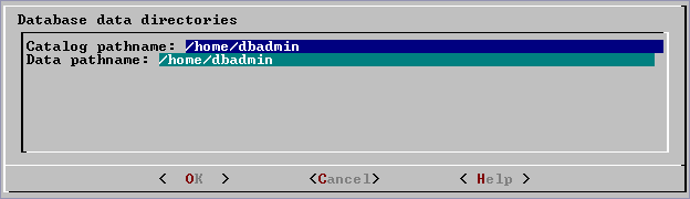
Specify the directories in which to store the data and catalog files, and click OK.
Note
Do not use a shared directory for more than one node. Data and catalog directories must be distinct for each node. Multiple nodes must not be allowed to write to the same data or catalog directory.
-
Catalog and data path names must contain only alphanumeric characters and cannot have leading spaces. Failure to comply with these restrictions results in database creation failure.
For example:
Catalog pathname: /home/dbadmin
Data Pathname: /home/dbadmin
-
Review the Current Database Definition screen to verify that it represents the database you want to create, and then click Yes to proceed or No to modify the database definition.
-
If you click Yes, Vertica creates the database you defined and then displays a message to indicate that the database was successfully created.
Note
: For databases created with 3 or more nodes, Vertica automatically sets
K-safety to 1 to ensure that the database is fault tolerant in case a node fails. For more information, see
Failure recovery in the Administrator's Guide and
MARK_DESIGN_KSAFE.
-
Click OK to acknowledge the message.
3.1.9 - Create the logical schema
Connect to the database.
-
Connect to the database.
In the Administration Tools Main Menu, click Connect to Database and click OK.
See Connecting to the Database for details.
The vsql welcome script appears:
Welcome to vsql, the Vertica Analytic Database interactive terminal.
Type:  \h or \? for help with vsql commands
       \g or terminate with semicolon to execute query
       \q to quit

=>
-
Run the logical schema script
Using the \i meta-command in vsql to run the SQL logical schema script that you prepared earlier.
-
Disconnect from the database
Use the \q meta-command in vsql to return to the Administration Tools.
3.1.10 - Perform a partial data load
Vertica recommends that for large tables, you perform a partial data load and then test your database before completing a full data load.
Vertica recommends that for large tables, you perform a partial data load and then test your database before completing a full data load. This load should load a representative amount of data.
-
Load the small tables.
Load the small table data files using the SQL load scripts and data files you prepared earlier.
-
Partially load the large tables.
Load 10GB to 50GB of table data for each table using the SQL load scripts and data files that you prepared earlier.
For more information about projections, see Projections.
3.1.11 - Test the database
Test the database to verify that it is running as expected.
Test the database to verify that it is running as expected.
Check queries for syntax errors and execution times.
-
Use the vsql \timing meta-command to enable the display of query execution time in milliseconds.
-
Execute the SQL sample query script that you prepared earlier.
-
Execute several ad hoc queries.
3.1.12 - Optimize query performance
Optimizing the database consists of optimizing for compression and tuning for queries.
Optimizing the database consists of optimizing for compression and tuning for queries. (See Creating a database design.)
To optimize the database, use the Database Designer to create and deploy a design for optimizing the database. See Using Database Designer to create a comprehensive design.
After you run the Database Designer, use the techniques described in Query optimization to improve the performance of certain types of queries.
Note
The database response time depends on factors such as type and size of the application query, database design, data size and data types stored, available computational power, and network bandwidth. Adding nodes to a database cluster does not necessarily improve the system response time for every query, especially if the response time is already short, e.g., less then 10 seconds, or the response time is not hardware bound.
3.1.13 - Complete the data load
To complete the load:.
To complete the load:
-
Monitor system resource usage.
Continue to run the top, free, and df utilities and watch them while your load scripts are running (as described in Monitoring Linux resource usage). You can do this on any or all nodes in the cluster. Make sure that the system is not swapping excessively (watch kswapd in top) or running out of swap space (watch for a large amount of used swap space in free).
Note
Vertica requires a dedicated server. If your loader or other processes take up significant amounts of RAM, it can result in swapping.
-
Complete the large table loads.
Run the remainder of the large table load scripts.
3.1.14 - Test the optimized database
Check query execution times to test your optimized design:.
Check query execution times to test your optimized design:
-
Use the vsql \timing meta-command to enable the display of query execution time in milliseconds.
Execute a SQL sample query script to test your schema and load scripts for errors.
Note
Include a sample of queries your users are likely to run against the database. If you don't have any real queries, just write simple SQL that collects counts on each of your tables. Alternatively, you can skip this step.
-
Execute several ad hoc queries
-
Run Administration tools and select Connect to Database.
-
Use the \i meta-command to execute the query script; for example:
vmartdb=> \i vmart_query_03.sql  customer_name   | annual_income
------------------+---------------
 James M. McNulty |        999979
 Emily G. Vogel   |        999998
(2 rows)
Time: First fetch (2 rows): 58.411 ms. All rows formatted: 58.448 ms
vmartdb=> \i vmart_query_06.sql
 store_key | order_number | date_ordered
-----------+--------------+--------------
        45 |       202416 | 2004-01-04
       113 |        66017 | 2004-01-04
       121 |       251417 | 2004-01-04
        24 |       250295 | 2004-01-04
         9 |       188567 | 2004-01-04
       166 |        36008 | 2004-01-04
        27 |       150241 | 2004-01-04
       148 |       182207 | 2004-01-04
       198 |        75716 | 2004-01-04
(9 rows)
Time: First fetch (9 rows): 25.342 ms. All rows formatted: 25.383 ms
Once the database is optimized, it should run queries efficiently. If you discover queries that you want to optimize, you can modify and update the design incrementally.
3.1.15 - Implement locales for international data sets
Vertica uses the ICU library for locale support; you must specify locale using the ICU locale syntax.
Locale specifies the user's language, country, and any special variant preferences, such as collation. Vertica uses locale to determine the behavior of certain string functions. Locale also determines the collation for various SQL commands that require ordering and comparison, such as aggregate GROUP BY and ORDER BY clauses, joins, and the analytic ORDER BY clause.
The default locale for a Vertica database is en_US@collation=binary (English US). You can define a new default locale that is used for all sessions on the database. You can also override the locale for individual sessions. However, projections are always collated using the default en_US@collation=binary collation, regardless of the session collation. Any locale-specific collation is applied at query time.
If you set the locale to null, Vertica sets the locale to en_US_POSIX. You can set the locale back to the default locale and collation by issuing the vsql meta-command \locale. For example:
Note
=> set locale to '';
INFO 2567:  Canonical locale: 'en_US_POSIX'
Standard collation: 'LEN'
English (United States, Computer)
SET
=> \locale en_US@collation=binary;
INFO 2567:  Canonical locale: 'en_US'
Standard collation: 'LEN_KBINARY'
English (United States)
=>  \locale
en_US@collation-binary;
You can set locale through ODBC, JDBC, and ADO.net.
ICU locale support
Vertica uses the ICU library for locale support; you must specify locale using the ICU locale syntax. The locale used by the database session is not derived from the operating system (through the LANG variable), so Vertica recommends that you set the LANG for each node running vsql, as described in the next section.
While ICU library services can specify collation, currency, and calendar preferences, Vertica supports only the collation component. Any keywords not relating to collation are rejected. Projections are always collated using the en_US@collation=binary collation regardless of the session collation. Any locale-specific collation is applied at query time.
The SET DATESTYLE TO ... command provides some aspects of the calendar, but Vertica supports only dollars as currency.
Changing DB locale for a session
This examples sets the session locale to Thai.
-
At the operating-system level for each node running vsql, set the LANG variable to the locale language as follows:
export LANG=th_TH.UTF-8
Note
If setting the LANG= as shown does not work, the operating system support for locales may not be installed.
-
For each Vertica session (from ODBC/JDBC or vsql) set the language locale.
From vsql:
\locale th_TH
-
From ODBC/JDBC:
"SET LOCALE TO th_TH;"
-
In PUTTY (or ssh terminal), change the settings as follows:
settings > window > translation > UTF-8
-
Click Apply and then click Save.
All data loaded must be in UTF-8 format, not an ISO format, as described in Delimited data. Character sets like ISO 8859-1 (Latin1), which are incompatible with UTF-8, are not supported, so functions like SUBSTRING do not work correctly for multibyte characters. Thus, settings for locale should not work correctly. If the translation setting ISO-8859-11:2001 (Latin/Thai) works, the data is loaded incorrectly. To convert data correctly, use a utility program such as Linux
iconv.
Note
The maximum length parameter for VARCHAR and CHAR data type refers to the number of octets (bytes) that can be stored in that field, not the number of characters. When using multi-byte UTF-8 characters, make sure to size fields to accommodate from 1 to 4 bytes per character, depending on the data.
See also
3.1.15.1 - Specify the default locale for the database
After you start the database, the default locale configuration parameter, DefaultSessionLocale, sets the initial locale.
After you start the database, the default locale configuration parameter, DefaultSessionLocale, sets the initial locale. You can override this value for individual sessions.
To set the locale for the database, use the configuration parameter as follows:
=> ALTER DATABASE DEFAULT SET DefaultSessionLocale = 'ICU-locale-identifier';
For example:
=> ALTER DATABASE DEFAULT SET DefaultSessionLocale = 'en_GB';
3.1.15.2 - Override the default locale for a session
You can override the default locale for the current session in two ways:.
You can override the default locale for the current session in two ways:
-
VSQL command
\locale. For example:
=> \locale en_GBINFO:
INFO 2567:  Canonical locale: 'en_GB'
Standard collation: 'LEN'
English (United Kingdom)
-
SQL statement
SET LOCALE. For example:
=> SET LOCALE TO en_GB;
INFO 2567:  Canonical locale: 'en_GB'
Standard collation: 'LEN'
English (United Kingdom)
Both methods accept locale short and long forms. For example:
=> SET LOCALE TO LEN;
INFO 2567:  Canonical locale: 'en'
Standard collation: 'LEN'
English
=> \locale LEN
INFO 2567:  Canonical locale: 'en'
Standard collation: 'LEN'
English
See also
3.1.15.3 - Server versus client locale settings
Vertica differentiates database server locale settings from client application locale settings:.
Vertica differentiates database server locale settings from client application locale settings:
The following sections describe best practices to ensure predictable results.
Server locale
The server session locale should be set as described in Specify the default locale for the database. If locales vary across different sessions, set the server locale at the start of each session from your client.
vsql client
-
If the database does not have a default session locale, set the server locale for the session to the desired locale.
-
The locale setting in the terminal emulator where the vsql client runs should be set to be equivalent to session locale setting on the server side (ICU locale). By doing so, the data is collated correctly on the server and displayed correctly on the client.
-
All input data for vsql should be in UTF-8, and all output data is encoded in UTF-8
-
Vertica does not support non UTF-8 encodings and associated locale values; .
-
For instructions on setting locale and encoding, refer to your terminal emulator documentation.
ODBC clients
-
ODBC applications can be either in ANSI or Unicode mode. If the user application is Unicode, the encoding used by ODBC is UCS-2. If the user application is ANSI, the data must be in single-byte ASCII, which is compatible with UTF-8 used on the database server. The ODBC driver converts UCS-2 to UTF-8 when passing to the Vertica server and converts data sent by the Vertica server from UTF-8 to UCS-2.
-
If the user application is not already in UCS-2, the application must convert the input data to UCS-2, or unexpected results could occur. For example:
-
For non-UCS-2 data passed to ODBC APIs, when it is interpreted as UCS-2, it could result in an invalid UCS-2 symbol being passed to the APIs, resulting in errors.
-
The symbol provided in the alternate encoding could be a valid UCS-2 symbol. If this occurs, incorrect data is inserted into the database.
-
If the database does not have a default session locale, ODBC applications should set the desired server session locale using SQLSetConnectAttr (if different from database wide setting). By doing so, you get the expected collation and string functions behavior on the server.
JDBC and ADO.NET clients
-
JDBC and ADO.NET applications use a UTF-16 character set encoding and are responsible for converting any non-UTF-16 encoded data to UTF-16. The same cautions apply as for ODBC if this encoding is violated.
-
The JDBC and ADO.NET drivers convert UTF-16 data to UTF-8 when passing to the Vertica server and convert data sent by Vertica server from UTF-8 to UTF-16.
-
If there is no default session locale at the database level, JDBC and ADO.NET applications should set the correct server session locale by executing the SET LOCALE TO command in order to get the expected collation and string functions behavior on the server. For more information, see SET LOCALE.
3.1.16 - Using time zones with Vertica
Vertica uses the public-domain tz database (time zone database), which contains code and data that represent the history of local time for locations around the globe.
Vertica uses the public-domain tz database (time zone database), which contains code and data that represent the history of local time for locations around the globe. This database organizes time zone and daylight saving time data by partitioning the world into timezones whose clocks all agree on timestamps that are later than the POSIX Epoch (1970-01-01 00:00:00 UTC). Each timezone has a unique identifier. Identifiers typically follow the convention area/location, where area is a continent or ocean, and location is a specific location within the area—for example, Africa/Cairo, America/New_York, and Pacific/Honolulu.
Important
IANA acknowledge that 1970 is an arbitrary cutoff. They note the problems that face moving the cutoff earlier "due to the wide variety of local practices before computer timekeeping became prevalent." IANA's own description of the tz database suggests that users should regard historical dates and times, especially those that predate the POSIX epoch date, with a healthy measure of skepticism. For details, see
Theory and pragmatics of the tz code and data.
Vertica uses the TZ environment variable (if set) on each node for the default current time zone. Otherwise, Vertica uses the operating system time zone.
The TZ variable can be set by the operating system during login (see /etc/profile, /etc/profile.d, or /etc/bashrc) or by the user in .profile, .bashrc or .bash-profile. TZ must be set to the same value on each node when you start Vertica.
The following command returns the current time zone for your database:
=> SHOW TIMEZONE;
   name   |     setting
----------+------------------
 timezone | America/New_York
(1 row)
You can also set the time zone for a single session with SET TIME ZONE.
Conversion and storage of date/time data
There is no database default time zone. TIMESTAMPTZ (TIMESTAMP WITH TIMEZONE) data is converted from the current local time and stored as GMT/UTC (Greenwich Mean Time/Coordinated Universal Time).
When TIMESTAMPTZ data is used, data is converted back to the current local time zone, which might be different from the local time zone where the data was stored. This conversion takes into account daylight saving time (summer time), depending on the year and date to determine when daylight saving time begins and ends.
TIMESTAMP WITHOUT TIMEZONE data stores the timestamp as given, and retrieves it exactly as given. The current time zone is ignored. The same is true for TIME WITHOUT TIMEZONE. For TIME WITH TIMEZONE (TIMETZ), however, the current time zone setting is stored along with the given time, and that time zone is used on retrieval.
Note
Vertica recommends that you use TIMESTAMPTZ, not TIMETZ.
Querying data/time data
TIMESTAMPTZ uses the current time zone on both input and output, as in the following example:
=> CREATE TEMP TABLE s (tstz TIMESTAMPTZ);=> SET TIMEZONE TO 'America/New_York';
=> INSERT INTO s VALUES ('2009-02-01 00:00:00');
=> INSERT INTO s VALUES ('2009-05-12 12:00:00');
=> SELECT tstz AS 'Local timezone', tstz AT TIMEZONE 'America/New_York' AS 'America/New_York',
   tstz AT TIMEZONE 'GMT' AS 'GMT' FROM s;
     Local timezone     |  America/New_York   |         GMT
------------------------+---------------------+---------------------
 2009-02-01 00:00:00-05 | 2009-02-01 00:00:00 | 2009-02-01 05:00:00
 2009-05-12 12:00:00-04 | 2009-05-12 12:00:00 | 2009-05-12 16:00:00
(2 rows)
The -05 in the Local time zone column shows that the data is displayed in EST, while -04 indicates EDT. The other two columns show the TIMESTAMP WITHOUT TIMEZONE at the specified time zone.
The next example shows what happens if the current time zone is changed to GMT:
=> SET TIMEZONE TO 'GMT';=> SELECT tstz AS 'Local timezone', tstz AT TIMEZONE 'America/New_York' AS
   'America/New_York', tstz AT TIMEZONE 'GMT' as 'GMT' FROM s;
     Local timezone     |  America/New_York   |         GMT
------------------------+---------------------+---------------------
 2009-02-01 05:00:00+00 | 2009-02-01 00:00:00 | 2009-02-01 05:00:00
 2009-05-12 16:00:00+00 | 2009-05-12 12:00:00 | 2009-05-12 16:00:00
(2 rows)
The +00 in the Local time zone column indicates that TIMESTAMPTZ is displayed in GMT.
The approach of using TIMESTAMPTZ fields to record events captures the GMT of the event, as expressed in terms of the local time zone. Later, it allows for easy conversion to any other time zone, either by setting the local time zone or by specifying an explicit AT TIMEZONE clause.
The following example shows how TIMESTAMP WITHOUT TIMEZONE fields work in Vertica.
=> CREATE TEMP TABLE tnoz (ts TIMESTAMP);=> INSERT INTO tnoz VALUES('2009-02-01 00:00:00');
=> INSERT INTO tnoz VALUES('2009-05-12 12:00:00');
=> SET TIMEZONE TO 'GMT';
=> SELECT ts AS 'No timezone', ts AT TIMEZONE 'America/New_York' AS
   'America/New_York', ts AT TIMEZONE 'GMT' AS 'GMT' FROM tnoz;
      No timezone    |    America/New_York    |          GMT
---------------------+------------------------+------------------------
 2009-02-01 00:00:00 | 2009-02-01 05:00:00+00 | 2009-02-01 00:00:00+00
 2009-05-12 12:00:00 | 2009-05-12 16:00:00+00 | 2009-05-12 12:00:00+00
(2 rows)
The +00 at the end of a timestamp indicates that the setting is TIMESTAMP WITH TIMEZONE in GMT (the current time zone). The America/New_York column shows what the GMT setting was when you recorded the time, assuming you read a normal clock in the America/New_York time zone. What this shows is that if it is midnight in the America/New_York time zone, then it is 5 am GMT.
Note
00:00:00 Sunday February 1, 2009 in America/New_York converts to 05:00:00 Sunday February 1, 2009 in GMT.
The GMT column displays the GMT time, assuming the input data was captured in GMT.
If you don't set the time zone to GMT, and you use another time zone, for example America/New_York, then the results display in America/New_York with a -05 and -04, showing the difference between that time zone and GMT.
=> SET TIMEZONE TO 'America/New_York';
=> SHOW TIMEZONE;
    name   |     setting
 ----------+------------------
  timezone | America/New_York
 (1 row)
=> SELECT ts AS 'No timezone', ts AT TIMEZONE 'America/New_York' AS
   'America/New_York', ts AT TIMEZONE 'GMT' AS 'GMT' FROM tnoz;
      No timezone    |    America/New_York    |          GMT
---------------------+------------------------+------------------------
 2009-02-01 00:00:00 | 2009-02-01 00:00:00-05 | 2009-01-31 19:00:00-05
 2009-05-12 12:00:00 | 2009-05-12 12:00:00-04 | 2009-05-12 08:00:00-04
(2 rows)
In this case, the last column is interesting in that it returns the time in New York, given that the data was captured in GMT.
See also
3.1.17 - Change transaction isolation levels
By default, Vertica uses the READ COMMITTED isolation level for all sessions.
By default, Vertica uses the READ COMMITTED isolation level for all sessions. You can change the default isolation level for the database or for a given session.
A transaction retains its isolation level until it completes, even if the session's isolation level changes during the transaction. Vertica internal processes (such as the Tuple Mover and refresh operations) and DDL operations always run at the SERIALIZABLE isolation level to ensure consistency.
Database isolation level
The configuration parameter
TransactionIsolationLevel specifies the database isolation level, and is used as the default for all sessions. Use
ALTER DATABASE to change the default isolation level.For example:
=> ALTER DATABASE DEFAULT SET TransactionIsolationLevel = 'SERIALIZABLE';
ALTER DATABASE
=> ALTER DATABASE DEFAULT SET TransactionIsolationLevel = 'READ COMMITTED';
ALTER DATABASE
Changes to the database isolation level only apply to future sessions. Existing sessions and their transactions continue to use their original isolation level.
Use
SHOW CURRENT to view the database isolation level:
=> SHOW CURRENT TransactionIsolationLevel;
  level   |           name            |    setting
----------+---------------------------+----------------
 DATABASE | TransactionIsolationLevel | READ COMMITTED
(1 row)
Session isolation level
SET SESSION CHARACTERISTICS AS TRANSACTION changes the isolation level for a specific session. For example:
=> SET SESSION CHARACTERISTICS AS TRANSACTION ISOLATION LEVEL SERIALIZABLE;
SET
Use
SHOW to view the current session's isolation level:
=> SHOW TRANSACTION_ISOLATION;
See also
Transactions
3.2 - Configuration parameter management
For details about individual configuration parameters grouped by category, see Configuration Parameters.
Vertica supports a wide variety of configuration parameters that affect many facets of database behavior. These parameters can be set with the appropriate ALTER statements at one or more levels, listed here in descending order of precedence:
-
User (ALTER USER)
-
Session (ALTER SESSION)
-
Node (ALTER NODE)
-
Database (ALTER DATABASE)
You can query system table CONFIGURATION_PARAMETERS to obtain the current settings for all user-accessible parameters. For example, the following query obtains settings for partitioning parameters: their current and default values, which levels they can be set at, and whether changes require a database restart to take effect:
=> SELECT parameter_name, current_value, default_value, allowed_levels, change_requires_restart
      FROM configuration_parameters  WHERE parameter_name ILIKE '%partitioncount%';
    parameter_name    | current_value | default_value | allowed_levels | change_requires_restart
----------------------+---------------+---------------+----------------+-------------------------
 MaxPartitionCount    | 1024          | 1024          | NODE, DATABASE | f
 ActivePartitionCount | 1             | 1             | NODE, DATABASE | f
(2 rows)
For details about individual configuration parameters grouped by category, see Configuration parameters.
Setting and clearing configuration parameters
You change specific configuration parameters with the appropriate ALTER statements; the same statements also let you reset configuration parameters to their default values. For example, the following ALTER statements change ActivePartitionCount at the database level from 1 to 2 , and DisablePartitionCount at the session level from 0 to 1:
=> ALTER DATABASE DEFAULT SET ActivePartitionCount = 2;
ALTER DATABASE
=> ALTER SESSION SET DisableAutopartition = 1;
ALTER SESSION
=> SELECT parameter_name, current_value, default_value FROM configuration_parameters
      WHERE parameter_name IN ('ActivePartitionCount', 'DisableAutopartition');
    parameter_name    | current_value | default_value
----------------------+---------------+---------------
 ActivePartitionCount | 2             | 1
 DisableAutopartition | 1             | 0
(2 rows)
You can later reset the same configuration parameters to their default values:
=> ALTER DATABASE DEFAULT CLEAR ActivePartitionCount;
ALTER DATABASE
=> ALTER SESSION CLEAR DisableAutopartition;
ALTER DATABASE
=> SELECT parameter_name, current_value, default_value FROM configuration_parameters
      WHERE parameter_name IN ('ActivePartitionCount', 'DisableAutopartition');
    parameter_name    | current_value | default_value
----------------------+---------------+---------------
 DisableAutopartition | 0             | 0
 ActivePartitionCount | 1             | 1
(2 rows)
Caution
Vertica is designed to operate with minimal configuration changes. Be careful to change configuration parameters according to documented guidelines.
3.2.1 - Viewing configuration parameter values
You can view active configuration parameter values in two ways:.
You can view active configuration parameter values in two ways:
SHOW statements
Use the following SHOW statements to view active configuration parameters:
-
SHOW CURRENT: Returns settings of active configuration parameter values. Vertica checks settings at all levels, in the following ascending order of precedence:
If no values are set at any scope, SHOW CURRENT returns the parameter's default value.
-
SHOW DATABASE: Displays configuration parameter values set for the database.
-
SHOW USER: Displays configuration parameters set for the specified user, and for all users.
-
SHOW SESSION: Displays configuration parameter values set for the current session.
-
SHOW NODE: Displays configuration parameter values set for a node.
If a configuration parameter requires a restart to take effect, the values in a SHOW CURRENT statement might differ from values in other SHOW statements. To see which parameters require restart, query the CONFIGURATION_PARAMETERS system table.
System tables
You can query several system tables for configuration parameters:
3.3 - Designing a logical schema
Designing a logical schema for a Vertica database is the same as designing for any other SQL database.
Designing a logical schema for a Vertica database is the same as designing for any other SQL database. A logical schema consists of objects such as schemas, tables, views and referential Integrity constraints that are visible to SQL users. Vertica supports any relational schema design that you choose.
3.3.1 - Using multiple schemas
Using a single schema is effective if there is only one database user or if a few users cooperate in sharing the database.
Using a single schema is effective if there is only one database user or if a few users cooperate in sharing the database. In many cases, however, it makes sense to use additional schemas to allow users and their applications to create and access tables in separate namespaces. For example, using additional schemas allows:
-
Many users to access the database without interfering with one another.
Individual schemas can be configured to grant specific users access to the schema and its tables while restricting others.
-
Third-party applications to create tables that have the same name in different schemas, preventing table collisions.
Unlike other RDBMS, a schema in a Vertica database is not a collection of objects bound to one user.
3.3.1.1 - Multiple schema examples
This section provides examples of when and how you might want to use multiple schemas to separate database users.
This section provides examples of when and how you might want to use multiple schemas to separate database users. These examples fall into two categories: using multiple private schemas and using a combination of private schemas (i.e. schemas limited to a single user) and shared schemas (i.e. schemas shared across multiple users).
Using multiple private schemas
Using multiple private schemas is an effective way of separating database users from one another when sensitive information is involved. Typically a user is granted access to only one schema and its contents, thus providing database security at the schema level. Database users can be running different applications, multiple copies of the same application, or even multiple instances of the same application. This enables you to consolidate applications on one database to reduce management overhead and use resources more effectively. The following examples highlight using multiple private schemas.
Using multiple schemas to separate users and their unique applications
In this example, both database users work for the same company. One user (HRUser) uses a Human Resource (HR) application with access to sensitive personal data, such as salaries, while another user (MedUser) accesses information regarding company healthcare costs through a healthcare management application. HRUser should not be able to access company healthcare cost information and MedUser should not be able to view personal employee data.
To grant these users access to data they need while restricting them from data they should not see, two schemas are created with appropriate user access, as follows:
Using multiple schemas to support multitenancy
This example is similar to the last example in that access to sensitive data is limited by separating users into different schemas. In this case, however, each user is using a virtual instance of the same application.
An example of this is a retail marketing analytics company that provides data and software as a service (SaaS) to large retailers to help them determine which promotional methods they use are most effective at driving customer sales.
In this example, each database user equates to a retailer, and each user only has access to its own schema. The retail marketing analytics company provides a virtual instance of the same application to each retail customer, and each instance points to the user’s specific schema in which to create and update tables. The tables in these schemas use the same names because they are created by instances of the same application, but they do not conflict because they are in separate schemas.
Example of schemas in this database could be:
-
MartSchema—A schema owned by MartUser, a large department store chain.
-
PharmSchema—A schema owned by PharmUser, a large drug store chain.
Using multiple schemas to migrate to a newer version of an application
Using multiple schemas is an effective way of migrating to a new version of a software application. In this case, a new schema is created to support the new version of the software, and the old schema is kept as long as necessary to support the original version of the software. This is called a “rolling application upgrade.”
For example, a company might use a HR application to store employee data. The following schemas could be used for the original and updated versions of the software:
-
HRSchema—A schema owned by HRUser, the schema user for the original HR application.
-
V2HRSchema—A schema owned by V2HRUser, the schema user for the new version of the HR application.
Combining private and shared schemas
The previous examples illustrate cases in which all schemas in the database are private and no information is shared between users. However, users might want to share common data. In the retail case, for example, MartUser and PharmUser might want to compare their per store sales of a particular product against the industry per store sales average. Since this information is an industry average and is not specific to any retail chain, it can be placed in a schema on which both users are granted USAGE privileges.
Example of schemas in this database might be:
-
MartSchema—A schema owned by MartUser, a large department store chain.
-
PharmSchema—A schema owned by PharmUser, a large drug store chain.
-
IndustrySchema—A schema owned by DBUser (from the retail marketing analytics company) on which both MartUser and PharmUser have USAGE privileges. It is unlikely that retailers would be given any privileges beyond USAGE on the schema and SELECT on one or more of its tables.
3.3.1.2 - Creating schemas
You can create as many schemas as necessary for your database.
You can create as many schemas as necessary for your database. For example, you could create a schema for each database user. However, schemas and users are not synonymous as they are in Oracle.
By default, only a superuser can create a schema or give a user the right to create a schema. (See GRANT (database) in the SQL Reference Manual.)
To create a schema use the CREATE SCHEMA statement, as described in the SQL Reference Manual.
3.3.1.3 - Specifying objects in multiple schemas
Once you create two or more schemas, each SQL statement or function must identify the schema associated with the object you are referencing.
Once you create two or more schemas, each SQL statement or function must identify the schema associated with the object you are referencing. You can specify an object within multiple schemas by:
-
Qualifying the object name by using the schema name and object name separated by a dot. For example, to specify MyTable, located in Schema1, qualify the name as Schema1.MyTable.
-
Using a search path that includes the desired schemas when a referenced object is unqualified. By Setting search paths, Vertica will automatically search the specified schemas to find the object.
3.3.1.4 - Setting search paths
Each user session has a search path of schemas.
Each user session has a search path of schemas. Vertica uses this search path to find tables and user-defined functions (UDFs) that are unqualified by their schema name. A session search path is initially set from the user's profile. You can change the session's search path at any time by calling
SET SEARCH_PATH. This search path remains in effect until the next SET SEARCH_PATH statement, or the session ends.
Viewing the current search path
SHOW SEARCH_PATH returns the session's current search path. For example:
=> SHOW SEARCH_PATH;
    name     |                      setting
-------------+---------------------------------------------------
 search_path | "$user", public, v_catalog, v_monitor, v_internal
Schemas are listed in descending order of precedence. The first schema has the highest precedence in the search order. If this schema exists, it is also defined as the current schema, which is used for tables that are created with unqualified names. You can identify the current schema by calling the function
CURRENT_SCHEMA:
=> SELECT CURRENT_SCHEMA;
 current_schema
----------------
 public
(1 row)
Setting the user search path
A session search path is initially set from the user's profile. If the search path in a user profile is not set by
CREATE USER or
ALTER USER, it is set to the database default:
=> CREATE USER agent007;
CREATE USER
=> \c - agent007
You are now connected as user "agent007".
=> SHOW SEARCH_PATH;
    name     |                      setting
-------------+---------------------------------------------------
 search_path | "$user", public, v_catalog, v_monitor, v_internal
$user resolves to the session user name—in this case, agent007—and has the highest precedence. If a schema agent007, exists, Vertica begins searches for unqualified tables in that schema. Also, calls to
CURRENT_SCHEMA return this schema. Otherwise, Vertica uses public as the current schema and begins searches in it.
Use
ALTER USER to modify an existing user's search path. These changes overwrite all non-system schemas in the search path, including $USER. System schemas are untouched. Changes to a user's search path take effect only when the user starts a new session; current sessions are unaffected.
For example, the following statements modify agent007's search path, and grant access privileges to schemas and tables that are on the new search path:
=> ALTER USER agent007 SEARCH_PATH store, public;
ALTER USER
=> GRANT ALL ON SCHEMA store, public TO agent007;
GRANT PRIVILEGE
=> GRANT SELECT ON ALL TABLES IN SCHEMA store, public TO agent007;
GRANT PRIVILEGE
=> \c - agent007
You are now connected as user "agent007".
=> SHOW SEARCH_PATH;
    name     |                     setting
-------------+-------------------------------------------------
 search_path | store, public, v_catalog, v_monitor, v_internal
(1 row)
To verify a user's search path, query the system table
USERS:
=> SELECT search_path FROM USERS WHERE user_name='agent007';
                   search_path
-------------------------------------------------
 store, public, v_catalog, v_monitor, v_internal
(1 row)
To revert a user's search path to the database default settings, call ALTER USER and set the search path to DEFAULT. For example:
=> ALTER USER agent007 SEARCH_PATH DEFAULT;
ALTER USER
=> SELECT search_path FROM USERS WHERE user_name='agent007';
                    search_path
---------------------------------------------------
 "$user", public, v_catalog, v_monitor, v_internal
(1 row)
Ignored search path schemas
Vertica only searches among existing schemas to which the current user has access privileges. If a schema in the search path does not exist or the user lacks access privileges to it, Vertica silently excludes it from the search. For example, if agent007 lacks SELECT privileges to schema public, Vertica silently skips this schema. Vertica returns with an error only if it cannot find the table anywhere on the search path.
Setting session search path
Vertica initially sets a session's search path from the user's profile. You can change the current session's search path with
SET SEARCH_PATH. You can use SET SEARCH_PATH in two ways:
-
Explicitly set the session search path to one or more schemas. For example:
=> \c - agent007
You are now connected as user "agent007".
dbadmin=> SHOW SEARCH_PATH;
    name     |                      setting
-------------+---------------------------------------------------
 search_path | "$user", public, v_catalog, v_monitor, v_internal
(1 row)

=> SET SEARCH_PATH TO store, public;
SET
=> SHOW SEARCH_PATH;
    name     |                     setting
-------------+-------------------------------------------------
 search_path | store, public, v_catalog, v_monitor, v_internal
(1 row)
-
Set the session search path to the database default:
=> SET SEARCH_PATH TO DEFAULT;
SET
=> SHOW SEARCH_PATH;
    name     |                      setting
-------------+---------------------------------------------------
 search_path | "$user", public, v_catalog, v_monitor, v_internal
(1 row)
SET SEARCH_PATH overwrites all non-system schemas in the search path, including $USER. System schemas are untouched.
3.3.1.5 - Creating objects that span multiple schemas
Vertica supports that reference tables across multiple schemas.
Vertica supports views that reference tables across multiple schemas. For example, a user might need to compare employee salaries to industry averages. In this case, the application queries two schemas:
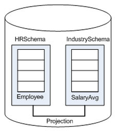
Best Practice: When creating objects that span schemas, use qualified table names. This naming convention avoids confusion if the query path or table structure within the schemas changes at a later date.
3.3.2 - Tables in schemas
In Vertica you can create persistent and temporary tables, through CREATE TABLE and CREATE TEMPORARY TABLE, respectively.
In Vertica you can create persistent and temporary tables, through
CREATE TABLE and
CREATE TEMPORARY TABLE, respectively.
For detailed information on both types, see Creating Tables and Creating temporary tables.
Persistent tables
CREATE TABLE creates a table in the Vertica logical schema. For example:
CREATE TABLE vendor_dimension (
   vendor_key        INTEGER      NOT NULL PRIMARY KEY,
   vendor_name       VARCHAR(64),
   vendor_address    VARCHAR(64),
   vendor_city       VARCHAR(64),
   vendor_state      CHAR(2),
   vendor_region     VARCHAR(32),
   deal_size         INTEGER,
   last_deal_update  DATE

);
For detailed information, see Creating Tables.
Temporary tables
CREATE TEMPORARY TABLE creates a table whose data persists only during the current session. Temporary table data is never visible to other sessions.
Temporary tables can be used to divide complex query processing into multiple steps. Typically, a reporting tool holds intermediate results while reports are generated—for example, the tool first gets a result set, then queries the result set, and so on.
CREATE TEMPORARY TABLE can create tables at two scopes, global and local, through the keywords GLOBAL and LOCAL, respectively:
-
GLOBAL (default): The table definition is visible to all sessions. However, table data is session-scoped.
-
LOCAL: The table definition is visible only to the session in which it is created. When the session ends, Vertica automatically drops the table.
For detailed information, see Creating temporary tables.
3.4 - Creating a database design
A is a physical storage plan that optimizes query performance.
A design is a physical storage plan that optimizes query performance. Data in Vertica is physically stored in projections. When you initially load data into a table using INSERT, COPY (or COPY LOCAL), Vertica creates a default superprojection for the table. This superprojection ensures that all of the data is available for queries. However, these superprojections might not optimize database performance, resulting in slow query performance and low data compression.
To improve performance, create a design for your Vertica database that optimizes query performance and data compression. You can create a design in several ways:
Database Designer can help you minimize how much time you spend on manual database tuning. You can also use Database Designer to redesign the database incrementally as requirements such as workloads change over time.
Database Designer runs as a background process. This is useful if you have a large design that you want to run overnight. An active SSH session is not required, so design and deploy operations continue to run uninterrupted if the session ends.
Tip
Vertica recommends that you first globally optimize your database using the Comprehensive setting in Database Designer. If the performance of the comprehensive design is not adequate, you can design custom projections using an incremental design and manually, as described in
Creating custom designs.
3.4.1 - About Database Designer
Vertica Database Designer uses sophisticated strategies to create a design that provides excellent performance for ad-hoc queries and specific queries while using disk space efficiently.
Vertica Database Designer uses sophisticated strategies to create a design that provides excellent performance for ad-hoc queries and specific queries while using disk space efficiently.
During the design process, Database Designer analyzes the logical schema definition, sample data, and sample queries, and creates a physical schema (projections) in the form of a SQL script that you deploy automatically or manually. This script creates a minimal set of superprojections to ensure K-safety.
In most cases, the projections that Database Designer creates provide excellent query performance within physical constraints while using disk space efficiently.
General design options
When you run Database Designer, several general options are available:
-
Create a comprehensive or incremental design.
-
Optimize for query execution, load, or a balance of both.
-
Require K-safety.
-
Recommend unsegmented projections when feasible.
-
Analyze statistics before creating the design.
Database Designer bases its design on the following information that you provide:
Output
Database Designer yields the following output:
-
Design script that creates the projections for the design in a way that meets the optimization objectives and distributes data uniformly across the cluster.
-
Deployment script that creates and refreshes the projections for your design. For comprehensive designs, the deployment script contains commands that remove non-optimized projections. The deployment script includes the full design script.
-
Backup script that contains SQL statements to deploy the design that existed on the system before deployment. This file is useful in case you need to revert to the pre-deployment design.
Design restrictions
Database Designer-generated designs:
-
Exclude live aggregate or Top-K projections. You must create these manually. See CREATE PROJECTION.
-
Do not sort, segment, or partition projections on LONG VARBINARY and LONG VARCHAR columns.
-
Do not support operations on complex types.
Post-design options
While running Database Designer, you can choose to deploy your design automatically after the deployment script is created, or to deploy it manually, after you have reviewed and tested the design. Vertica recommends that you test the design on a non-production server before deploying the design to your production server.
3.4.2 - How Database Designer creates a design
Database Designer-generated designs can include the following recommendations:.
Design recommendations
Database Designer-generated designs can include the following recommendations:
-
Sort buddy projections in the same order, which can significantly improve load, recovery, and site node performance. All buddy projections have the same base name so that they can be identified as a group.
Note
If you manually create projections, Database Designer recommends a buddy with the same sort order, if one does not already exist. By default, Database Designer recommends both super and non-super segmented projections with a buddy of the same sort order and segmentation.
-
Accepts unlimited queries for a comprehensive design.
-
Identifies similar design queries and assigns them a signature.
For queries with the same signature, Database Designer weights the queries, depending on how many queries have that signature. It then considers the weighted query when creating a design.
-
Recommends and creates projections in a way that minimizes data skew by distributing data uniformly across the cluster.
-
Produces higher quality designs by considering UPDATE, DELETE, and SELECT statements.
3.4.3 - Database Designer access requirements
By default, only users with the DBADMIN role can run Database Designer.
By default, only users with the DBADMIN role can run Database Designer. Non-DBADMIN users can run Database Designer only if they are granted the necessary privileges and DBDUSER role, as described below. You can also enable users to run Database Designer on the Management Console (see Enabling Users to run Database Designer on Management Console).
-
Add a temporary folder to all cluster nodes with CREATE LOCATION:
=> CREATE LOCATION '/tmp/dbd' ALL NODES;
-
Grant the desired user CREATE privileges to create schemas on the current (DEFAULT) database, with GRANT DATABASE:
=> GRANT CREATE ON DATABASE DEFAULT TO dbd-user;
-
Grant the DBDUSER role to dbd-user with GRANT ROLE:
=> GRANT DBDUSER TO dbd-user;
-
On all nodes in the cluster, grant dbd-user access to the temporary folder with GRANT LOCATION:
=> GRANT ALL ON LOCATION '/tmp/dbd' TO dbd-user;
-
Grant dbd-user privileges on one or more database schemas and their tables, with GRANT SCHEMA and GRANT TABLE, respectively:
=> GRANT ALL ON SCHEMA this-schema[,...] TO dbd-user;
=> GRANT ALL ON ALL TABLES IN SCHEMA this-schema[,...] TO dbd-user;
-
Enable the DBDUSER role on dbd-user in one of the following ways:
-
As dbd-user, enable the DBDUSER role with SET ROLE:
=> SET ROLE DBDUSER;
-
As DBADMIN, automatically enable the DBDUSER role for dbd-user on each login, with ALTER USER:
=> ALTER USER dbd-user DEFAULT ROLE DBDUSER;
Important
When you grant the DBDUSER role, be sure to associate a resource pool with that user to manage resources while Database Designer runs.
Multiple users can run Database Designer concurrently without interfering with each other or exhausting cluster resources. When a user runs Database Designer, either with Management Console or programmatically, execution is generally contained by the user's resource pool, but might spill over into system resource pools for less-intensive tasks.
Enabling users to run Database Designer on Management Console
Users who are already granted the DBDUSER role and required privileges, as described above, can also be enabled to run Database Designer on Management Console:
-
Log in as a superuser to Management Console.
-
Click MC Settings.
-
Click User Management.
-
Specify an MC user:
-
To create an MC user, click Add.
-
To use an existing MC user, select the user and click Edit.
-
Next to the DB access level window, click Add.
-
In the Add Permissions window:
-
From the Choose a database drop-down list, select the database on which to create a design.
-
In the Database username field, enter the dbd-user user name that you created earlier.
-
In the Database password field, enter the database password.
-
In the Restrict access drop-down list, select the level of MC user for this user.
-
Click OK to save your changes.
-
Log out of the MC Super user account.
The MC user is now mapped to dbd-user. Log in as the MC user and use Database Designer to create an optimized design for your database.
DBDUSER capabilities and limitations
As a DBDUSER, the following constraints apply:
-
Designs must set K-safety to be equal to system K-safety. If a design violates K-safety by lacking enough buddy projections for tables, the design does not complete.
-
You cannot explicitly advance the ancient history mark (AHM)—for example, call MAKE_AHM_NOW—until after deploying the design.
When you create a design, you automatically have privileges to manipulate that design. Other tasks might require additional privileges:
|
Task |
Required privileges |
|
Submit design tables |
|
|
Submit a single design query |
- EXECUTE on the design query
|
|
Submit a file of design queries |
|
|
Submit design queries from results of a user query |
|
|
Create design and deployment scripts |
|
3.4.4 - Logging projection data for Database Designer
When you run Database Designer, the Optimizer proposes a set of ideal projections based on the options that you specify.
When you run Database Designer, the Optimizer proposes a set of ideal projections based on the options that you specify. When you deploy the design, Database Designer creates the design based on these projections. However, space or budget constraints may prevent Database Designer from creating all the proposed projections. In addition, Database Designer may not be able to implement the projections using ideal criteria.
To get information about the projections, first enable the Database Designer logging capability. When enabled, Database Designer stores information about the proposed projections in two Data Collector tables. After Database Designer deploys the design, these logs contain information about which proposed projections were actually created. After deployment, the logs contain information about:
-
Projections that the Optimizer proposed
-
Projections that Database Designer actually created when the design was deployed
-
Projections that Database Designer created, but not with the ideal criteria that the Optimizer identified.
-
The DDL used to create all the projections
-
Column optimizations
If you do not deploy the design immediately, review the log to determine if you want to make any changes. If the design has been deployed, you can still manually create some of the projections that Database Designer did not create.
To enable the Database Designer logging capability, see Enabling logging for Database Designer.
To view the logged information, see Viewing Database Designer logs.
3.4.4.1 - Enabling logging for Database Designer
By default, Database Designer does not log information about the projections that the Optimizer proposed and the Database Designer deploys.
By default, Database Designer does not log information about the projections that the Optimizer proposed and the Database Designer deploys.
To enable Database Designer logging, enter the following command:
=> ALTER DATABASE DEFAULT SET DBDLogInternalDesignProcess = 1;
To disable Database Designer logging, enter the following command:
=> ALTER DATABASE DEFAULT SET DBDLogInternalDesignProcess = 0;
See also
3.4.4.2 - Viewing Database Designer logs
You can find data about the projections that Database Designer considered and deployed in two Data Collector tables:.
You can find data about the projections that Database Designer considered and deployed in two Data Collector tables:
DC_DESIGN_PROJECTION_CANDIDATES
The DC_DESIGN_PROJECTION_CANDIDATES table contains information about all the projections that the Optimizer proposed. This table also includes the DDL that creates them. The is_a_winner field indicates if that projection was part of the actual deployed design. To view the DC_DESIGN_PROJECTION_CANDIDATES table, enter:
=> SELECT * FROM DC_DESIGN_PROJECTION_CANDIDATES;
DC_DESIGN_QUERY_PROJECTION_CANDIDATES
The DC_DESIGN_QUERY_PROJECTION_CANDIDATES table lists plan features for all design queries.
Possible features are:
For all design queries, the DC_DESIGN_QUERY_PROJECTION_CANDIDATES table includes the following plan feature information:
-
Optimizer path cost.
-
Database Designer benefits.
-
Ideal plan feature and its description, which identifies how the referenced projection should be optimized.
-
If the design was deployed, the actual plan feature and its description is included in the table. This information identifies how the referenced projection was actually optimized.
Because most projections have multiple optimizations, each projection usually has multiple rows.To view the DC_DESIGN_QUERY_PROJECTION_CANDIDATES table, enter:
=> SELECT * FROM DC_DESIGN_QUERY_PROJECTION_CANDIDATES;
To see example data from these tables, see Database Designer logs: example data.
3.4.4.3 - Database Designer logs: example data
In the following example, Database Designer created the logs after creating a comprehensive design for the VMart sample database.
In the following example, Database Designer created the logs after creating a comprehensive design for the VMart sample database. The output shows two records from the DC_DESIGN_PROJECTION_CANDIDATES table.
The first record contains information about the customer_dimension_dbd_1_sort_$customer_gender$__$annual_income$ projection. The record includes the CREATE PROJECTION statement that Database Designer used to create the projection. The is_a_winner column is t, indicating that Database Designer created this projection when it deployed the design.
The second record contains information about the product_dimension_dbd_2_sort_$product_version$__$product_key$ projection. For this projection, the is_a_winner column is f. The Optimizer recommended that Database Designer create this projection as part of the design. However, Database Designer did not create the projection when it deployed the design. The log includes the DDL for the CREATE PROJECTION statement. If you want to add the projection manually, you can use that DDL. For more information, see Creating a design manually.
=> SELECT * FROM dc_design_projection_candidates;
-[ RECORD 1 ]--------+---------------------------------------------------------------
time                 | 2014-04-11 06:30:17.918764-07
node_name            | v_vmart_node0001
session_id           | localhost.localdoma-931:0x1b7
user_id              | 45035996273704962
user_name            | dbadmin
design_id            | 45035996273705182
design_table_id      | 45035996273720620
projection_id        | 45035996273726626
iteration_number     | 1
projection_name      | customer_dimension_dbd_1_sort_$customer_gender$__$annual_income$
projection_statement | CREATE PROJECTION v_dbd_sarahtest_sarahtest."customer_dimension_dbd_1_
            sort_$customer_gender$__$annual_income$"
(
customer_key ENCODING AUTO,
customer_type ENCODING AUTO,
customer_name ENCODING AUTO,
customer_gender ENCODING RLE,
title ENCODING AUTO,
household_id ENCODING AUTO,
customer_address ENCODING AUTO,
customer_city ENCODING AUTO,
customer_state ENCODING AUTO,
customer_region ENCODING AUTO,
marital_status ENCODING AUTO,
customer_age ENCODING AUTO,
number_of_children ENCODING AUTO,
annual_income ENCODING AUTO,
occupation ENCODING AUTO,
largest_bill_amount ENCODING AUTO,
store_membership_card ENCODING AUTO,
customer_since ENCODING AUTO,
deal_stage ENCODING AUTO,
deal_size ENCODING AUTO,
last_deal_update ENCODING AUTO
)
AS
SELECT customer_key,
customer_type,
customer_name,
customer_gender,
title,
household_id,
customer_address,
customer_city,
customer_state,
customer_region,
marital_status,
customer_age,
number_of_children,
annual_income,
occupation,
largest_bill_amount,
store_membership_card,
customer_since,
deal_stage,
deal_size,
last_deal_update
FROM public.customer_dimension
ORDER BY customer_gender,
annual_income
UNSEGMENTED ALL NODES;
is_a_winner          | t
-[ RECORD 2 ]--------+-------------------------------------------------------------
time                 | 2014-04-11 06:30:17.961324-07
node_name            | v_vmart_node0001
session_id           | localhost.localdoma-931:0x1b7
user_id              | 45035996273704962
user_name            | dbadmin
design_id            | 45035996273705182
design_table_id      | 45035996273720624
projection_id        | 45035996273726714
iteration_number     | 1
projection_name      | product_dimension_dbd_2_sort_$product_version$__$product_key$
projection_statement | CREATE PROJECTION v_dbd_sarahtest_sarahtest."product_dimension_dbd_2_
        sort_$product_version$__$product_key$"
(
product_key ENCODING AUTO,
product_version ENCODING RLE,
product_description ENCODING AUTO,
sku_number ENCODING AUTO,
category_description ENCODING AUTO,
department_description ENCODING AUTO,
package_type_description ENCODING AUTO,
package_size ENCODING AUTO,
fat_content ENCODING AUTO,
diet_type ENCODING AUTO,
weight ENCODING AUTO,
weight_units_of_measure ENCODING AUTO,
shelf_width ENCODING AUTO,
shelf_height ENCODING AUTO,
shelf_depth ENCODING AUTO,
product_price ENCODING AUTO,
product_cost ENCODING AUTO,
lowest_competitor_price ENCODING AUTO,
highest_competitor_price ENCODING AUTO,
average_competitor_price ENCODING AUTO,
discontinued_flag ENCODING AUTO
)
AS
SELECT product_key,
product_version,
product_description,
sku_number,
category_description,
department_description,
package_type_description,
package_size,
fat_content,
diet_type,
weight,
weight_units_of_measure,
shelf_width,
shelf_height,
shelf_depth,
product_price,
product_cost,
lowest_competitor_price,
highest_competitor_price,
average_competitor_price,
discontinued_flag
FROM public.product_dimension
ORDER BY product_version,
product_key
UNSEGMENTED ALL NODES;
is_a_winner          | f
.
.
.
The next example shows the contents of two records in the DC_DESIGN_QUERY_PROJECTION_CANDIDATES. Both of these rows apply to projection id 45035996273726626.
In the first record, the Optimizer recommends that Database Designer optimize the customer_gender column for the GROUPBY PIPE algorithm.
In the second record, the Optimizer recommends that Database Designer optimize the public.customer_dimension table for late materialization. Late materialization can improve the performance of joins that might spill to disk.
=> SELECT * FROM dc_design_query_projection_candidates;
-[ RECORD 1 ]-----------------+------------------------------------------------------------
time                           | 2014-04-11 06:30:17.482377-07
node_name                      | v_vmart_node0001
session_id                     | localhost.localdoma-931:0x1b7
user_id                        | 45035996273704962
user_name                      | dbadmin
design_id                      | 45035996273705182
design_query_id                | 3
iteration_number               | 1
design_table_id                | 45035996273720620
projection_id                  | 45035996273726626
ideal_plan_feature             | GROUP BY PIPE
ideal_plan_feature_description | Group-by pipelined on column(s) customer_gender
dbd_benefits                   | 5
opt_path_cost                  | 211
-[ RECORD 2 ]-----------------+------------------------------------------------------------
time                           | 2014-04-11 06:30:17.48276-07
node_name                      | v_vmart_node0001
session_id                     | localhost.localdoma-931:0x1b7
user_id                        | 45035996273704962
user_name                      | dbadmin
design_id                      | 45035996273705182
design_query_id                | 3
iteration_number               | 1
design_table_id                | 45035996273720620
projection_id                  | 45035996273726626
ideal_plan_feature             | LATE MATERIALIZATION
ideal_plan_feature_description | Late materialization on table public.customer_dimension
dbd_benefits                   | 4
opt_path_cost                  | 669
.
.
.
You can view the actual plan features that Database Designer implemented for the projections it created. To do so, query the V_INTERNAL.DC_DESIGN_QUERY_PROJECTIONS table:
=> select * from v_internal.dc_design_query_projections;
-[ RECORD 1 ]-------------------+-------------------------------------------------------------
time                            | 2014-04-11 06:31:41.19199-07
node_name                       | v_vmart_node0001
session_id                      | localhost.localdoma-931:0x1b7
user_id                         | 45035996273704962
user_name                       | dbadmin
design_id                       | 45035996273705182
design_query_id                 | 1
projection_id                   | 2
design_table_id                 | 45035996273720624
actual_plan_feature             | RLE PREDICATE
actual_plan_feature_description | RLE on predicate column(s) department_description
dbd_benefits                    | 2
opt_path_cost                   | 141
-[ RECORD 2 ]-------------------+-------------------------------------------------------------
time                            | 2014-04-11 06:31:41.192292-07
node_name                       | v_vmart_node0001
session_id                      | localhost.localdoma-931:0x1b7
user_id                         | 45035996273704962
user_name                       | dbadmin
design_id                       | 45035996273705182
design_query_id                 | 1
projection_id                   | 2
design_table_id                 | 45035996273720624
actual_plan_feature             | GROUP BY PIPE
actual_plan_feature_description | Group-by pipelined on column(s) fat_content
dbd_benefits                    | 5
opt_path_cost                   | 155
3.4.5 - General design settings
Before you run Database Designer, you must provide specific information on the design to create.
Before you run Database Designer, you must provide specific information on the design to create.
Design name
All designs that you create with Database Designer must have unique names that conform to the conventions described in Identifiers, and are no more than 32 characters long (16 characters if you use Database Designer in Administration Tools or Management Console).
The design name is incorporated into the names of files that Database Designer generates, such as its deployment script. This can help you differentiate files that are associated with different designs.
Design type
Database Designer can create two distinct design types: comprehensive or incremental.
Comprehensive design
A comprehensive design creates an initial or replacement design for all the tables in the specified schemas. Create a comprehensive design when you are creating a new database.
To help Database Designer create an efficient design, load representative data into the tables before you begin the design process. When you load data into a table, Vertica creates an unoptimized superprojection so that Database Designer has projections to optimize. If a table has no data, Database Designer cannot optimize it.
Optionally, supply Database Designer with representative queries that you plan to use so Database Designer can optimize the design for them. If you do not supply any queries, Database Designer creates a generic optimization of the superprojections that minimizes storage, with no query-specific projections.
During a comprehensive design, Database Designer creates deployment scripts that:
Incremental design
After you create and deploy a comprehensive database design, your database is likely to change over time in various ways. Consider using Database Designer periodically to create incremental designs that address these changes. Changes that warrant an incremental design can include:
-
Significant data additions or updates
-
New or modified queries that you run regularly
-
Performance issues with one or more queries
-
Schema changes
Optimization objective
Database Designer can optimize the design for one of three objectives:
- Load: Designs that are optimized for loads minimize database size, potentially at the expense of query performance.
- Query: Designs that are optimized for query performance. These designs typically favor fast query execution over load optimization, and thus result in a larger storage footprint.
- Balanced: Designs that are balanced between database size and query performance.
A fully optimized query has an optimization ratio of 0.99. Optimization ratio is the ratio of a query's benefits achieved in the design produced by the Database Designer to that achieved in the ideal plan. The optimization ratio is set in the OptRatio parameter in designer.log.
Design tables
Database Designer needs one or more tables with a moderate amount of sample data—approximately 10 GB—to create optimal designs. Design tables with large amounts of data adversely affect Database Designer performance. Design tables with too little data prevent Database Designer from creating an optimized design. If a design table has no data, Database Designer ignores it.
Note
If you drop a table after adding it to the design, Database Designer cannot build or deploy the design.
Design queries
A database design that is optimized for query performance requires a set of representative queries, or design queries. Design queries are required for incremental designs, and optional for comprehensive designs. You list design queries in a SQL file that you supply as input to Database Designer. Database Designer checks the validity of the queries when you add them to your design, and again when it builds the design. If a query is invalid, Database Designer ignores it.
If you use Management Console to create a database design, you can submit queries either from an input file or from the system table QUERY_REQUESTS. For details, see Creating a design manually.
The maximum number of design queries depends on the design type: ≤200 queries for a comprehensive design, ≤100 queries for an incremental design. Optionally, you can assign weights to the design queries that signify their relative importance. Database Designer uses those weights to prioritize the queries in its design.
Segmented and unsegmented projections
When creating a comprehensive design, Database Designer creates projections based on data statistics and queries. It also reviews the submitted design tables to decide whether projections should be segmented (distributed across the cluster nodes) or unsegmented (replicated on all cluster nodes).
By default, Database Designer recommends only segmented projections. You can enable Database Designer to recommend unsegmented projections . In this case, Database Designer recommends segmented superprojections for large tables when deploying to multi-node clusters, and unsegmented superprojections for smaller tables.
Database Designer uses the following algorithm to determine whether to recommend unsegmented projections. Assuming that largest-row-count equals the number of rows in the design table with the largest number of rows, Database Designer recommends unsegmented projections if any of the following conditions is true:
-
largest-row-count< 1,000,000 ANDnumber-table-rows≤10%-largest-row-count
-
largest-row-count≥ 10,000,000 ANDnumber-table-rows≤1%-largest-row-count
-
1,000,000 ≤ largest-row-count< 10,000,000 ANDnumber-table-rows ≤ 100,000
Database Designer does not segment projections on:
For more information, see High availability with projections.
Statistics analysis
By default, Database Designer analyzes statistics for design tables when they are added to the design. Accurate statistics help Database Designer optimize compression and query performance.
Analyzing statistics takes time and resources. If you are certain that design table statistics are up to date, you can specify to skip this step and avoid the overhead otherwise incurred.
For more information, see Collecting Statistics.
3.4.6 - Building a design
After you have created design tables and loaded data into them, and then specified the parameters you want Database Designer to use when creating the physical schema, direct Database Designer to create the scripts necessary to build the design.
After you have created design tables and loaded data into them, and then specified the parameters you want Database Designer to use when creating the physical schema, direct Database Designer to create the scripts necessary to build the design.
Note
You cannot stop a running database if Database Designer is building a database design.
When you build a database design, Vertica generates two scripts:
-
Deployment script: design-name_deploy.sql—Contains the SQL statements that create projections for the design you are deploying, deploy the design, and drop unused projections. When the deployment script runs, it creates the optimized design. For details about how to run this script and deploy the design, see Deploying a Design.
-
Design script: design-name_design.sql—Contains the CREATE PROJECTION statements that Database Designeruses to create the design. Review this script to make sure you are happy with the design.
The design script is a subset of the deployment script. It serves as a backup of the DDL for the projections that the deployment script creates.
When you create a design using Management Console:
-
If you submit a large number of queries to your design and build it right immediately, a timing issue could cause the queries not to load before deployment starts. If this occurs, you might see one of the following errors:
To accommodate this timing issue, you may need to reset the design, check the Queries tab to make sure the queries have been loaded, and then rebuild the design. Detailed instructions are in:
-
The scripts are deleted when deployment completes. To save a copy of the deployment script after the design is built but before the deployment completes, go to the Output window and copy and paste the SQL statements to a file.
3.4.7 - Resetting a design
You must reset a design when:.
You must reset a design when:
-
You build a design and the output scripts described in Building a Design are not created.
-
You build a design but Database Designer cannot complete the design because the queries it expects are not loaded.
Resetting a design discards all the run-specific information of the previous Database Designer build, but retains its configuration (design type, optimization objectives, K-safety, etc.) and tables and queries.
After you reset a design, review the design to see what changes you need to make. For example, you can fix errors, change parameters, or check for and add additional tables or queries. Then you can rebuild the design.
You can only reset a design in Management Console or by using the DESIGNER_RESET_DESIGN function.
3.4.8 - Deploying a design
After running Database Designer to generate a deployment script, Vertica recommends that you test your design on a non-production server before you deploy it to your production server.
After running Database Designer to generate a deployment script, Vertica recommends that you test your design on a non-production server before you deploy it to your production server.
Both the design and deployment processes run in the background. This is useful if you have a large design that you want to run overnight. Because an active SSH session is not required, the design/deploy operations continue to run uninterrupted, even if the session is terminated.
Note
You cannot stop a running database if Database Designer is building or deploying a database design.
Database Designer runs as a background process. Multiple users can run Database Designer concurrently without interfering with each other or using up all the cluster resources. However, if multiple users are deploying a design on the same tables at the same time, Database Designer may not be able to complete the deployment. To avoid problems, consider the following:
-
Schedule potentially conflicting Database Designer processes to run sequentially overnight so that there are no concurrency problems.
-
Avoid scheduling Database Designer runs on the same set of tables at the same time.
There are two ways to deploy your design:
3.4.8.1 - Deploying designs using Database Designer
OpenText recommends that you run Database Designer and deploy optimized projections right after loading your tables with sample data because Database Designer provides projections optimized for the current state of your database.
OpenText recommends that you run Database Designer and deploy optimized projections right after loading your tables with sample data because Database Designer provides projections optimized for the current state of your database.
If you choose to allow Database Designer to automatically deploy your script during a comprehensive design and are running Administrative Tools, Database Designer creates a backup script of your database's current design. This script helps you re-create the design of projections that may have been dropped by the new design. The backup script is located in the output directory you specified during the design process.
If you choose not to have Database Designer automatically run the deployment script (for example, if you want to maintain projections from a pre-existing deployment), you can manually run the deployment script later. See Deploying designs manually.
To deploy a design while running Database Designer, do one of the following:
-
In Management Console, select the design and click Deploy Design.
-
In the Administration Tools, select Deploy design in the Design Options window.
If you are running Database Designer programmatically, use DESIGNER_RUN_POPULATE_DESIGN_AND_DEPLOY and set the deploy parameter to 'true'.
Once you have deployed your design, query the DEPLOY_STATUS system table to see the steps that the deployment took:
vmartdb=> SELECT * FROM V_MONITOR.DEPLOY_STATUS;
3.4.8.2 - Deploying designs manually
If you choose not to have Database Designer deploy your design at design time, you can deploy the design later using the deployment script:.
If you choose not to have Database Designer deploy your design at design time, you can deploy the design later using the deployment script:
-
Make sure that the target database contains the same tables and projections as the database where you ran Database Designer. The database should also contain sample data.
-
To deploy the projections to a test or production environment, execute the deployment script in vsql with the meta-command
\i as follows, where design‑name is the name of the database design:
=> \i design-name_deploy.sql
-
For a K-safe database, call Vertica meta-function
GET_PROJECTIONS on tables of the new projections. Check the output to verify that all projections have enough buddies to be identified as safe.
-
If you create projections for tables that already contains data, call
REFRESH or
START_REFRESH to update new projections. Otherwise, these projections are not available for query processing.
-
Call
MAKE_AHM_NOW to set the Ancient History Mark (AHM) to the most recent epoch.
-
Call
DROP PROJECTION on projections that are no longer needed, and would otherwise waste disk space and reduce load speed.
-
Call
ANALYZE_STATISTICS on all database projections:
=> SELECT ANALYZE_STATISTICS ('');
This function collects and aggregates data samples and storage information from all nodes on which a projection is stored, and then writes statistics into the catalog.
3.4.9 - How to create a design
There are three ways to create a design using Database Designer:.
There are three ways to create a design using Database Designer:
The following table shows what Database Designer capabilities are available in each tool:
|
Database Designer Capability |
Management Console |
Running Database Designer Programmatically |
Administrative Tools |
|
Create design |
Yes |
Yes |
Yes |
|
Design name length (# of characters) |
16 |
32 |
16 |
|
Build design (create design and deployment scripts) |
Yes |
Yes |
Yes |
|
Create backup script |
|
|
Yes |
|
Set design type (comprehensive or incremental) |
Yes |
Yes |
Yes |
|
Set optimization objective |
Yes |
Yes |
Yes |
|
Add design tables |
Yes |
Yes |
Yes |
|
Add design queries file |
Yes |
Yes |
Yes |
|
Add single design query |
|
Yes |
|
|
Use query repository |
Yes |
Yes |
|
|
Set K-safety |
Yes |
Yes |
Yes |
|
Analyze statistics |
Yes |
Yes |
Yes |
|
Require all unsegmented projections |
Yes |
Yes |
|
|
View event history |
Yes |
Yes |
|
|
Set correlation analysis mode (Default = 0) |
|
Yes |
|
3.4.9.1 - Using administration tools to create a design
To use the Administration Tools interface to create an optimized design for your database, you must be a DBADMIN user.
To use the Administration Tools interface to create an optimized design for your database, you must be a DBADMIN user. Follow these steps:
-
Log in as the dbadmin user and start Administration Tools.
-
From the main menu, start the database for which you want to create a design. The database must be running before you can create a design for it.
-
On the main menu, select Configuration Menu and click OK.
-
On the Configuration Menu, select Run Database Designer and click OK.
-
On the Select a database to design window, enter the name of the database for which you are creating a design and click OK.
-
On the Enter the directory for Database Designer output window, enter the full path to the directory to contain the design script, deployment script, backup script, and log files, and click OK.
For information about the scripts, see Building a design.
-
On the Database Designer window, enter a name for the design and click OK.
-
On the Design Type window, choose which type of design to create and click OK.
For details, see Design Types.
-
The Select schema(s) to add to query search path window lists all the schemas in the database that you selected. Select the schemas that contain representative data that you want Database Designer to consider when creating the design and click OK.
For details about choosing schema and tables to submit to Database Designer, see Design Tables with Sample Data.
-
On the Optimization Objectives window, select the objective you want for the database optimization:
-
The final window summarizes the choices you have made and offers you two choices:
-
Proceed with building the design, and deploying it if you specified to deploy it immediately. If you did not specify to deploy, you can review the design and deployment scripts and deploy them manually, as described in Deploying designs manually.
-
Cancel the design and go back to change some of the parameters as needed.
-
Creating a design can take a long time.To cancel a running design from the Administration Tools window, enter Ctrl+C.
To create a design for the VMart example database, see Using Database Designer to create a comprehensive design in Getting Started.
3.4.10 - Running Database Designer programmatically
Vertica provides a set of meta-functions that enable programmatic access to Database Designer functionality.
Vertica provides a set of meta-functions that enable programmatic access to Database Designer functionality. Run Database Designer programmatically to perform the following tasks:
-
Optimize performance on tables that you own.
-
Create or update a design without requiring superuser or DBADMIN intervention.
-
Add individual queries and tables, or add data to your design, and then rerun Database Designer to update the design based on this new information.
-
Customize the design.
-
Use recently executed queries to set up your database to run Database Designer automatically on a regular basis.
-
Assign each design query a query weight that indicates the importance of that query in creating the design. Assign a higher weight to queries that you run frequently so that Database Designer prioritizes those queries in creating the design.
For more details about Database Designer functions, see Database Designer function categories.
3.4.10.1 - Database Designer function categories
Database Designer functions perform the following operations, generally performed in the following order:
-
Create a design.
-
Set design properties.
-
Populate a design.
-
Create design and deployment scripts.
-
Get design data.
-
Clean up.
Important
You can also use meta-function
DESIGNER_SINGLE_RUN, which encapsulates all of these steps with a single call. The meta-function iterates over all queries within a specified timespan, and returns with a design ready for deployment.
For detailed information, see Workflow for running Database Designer programmatically. For information on required privileges, see Privileges for running Database Designer functions
Caution
Before running Database Designer functions on an existing schema, back up the current design by calling
EXPORT_CATALOG.
Create a design
DESIGNER_CREATE_DESIGN directs Database Designer to create a design.
Set design properties
The following functions let you specify design properties:
Populate a design
The following functions let you add tables and queries to your Database Designer design:
Create design and deployment scripts
The following functions populate the Database Designer workspace and create design and deployment scripts. You can also analyze statistics, deploy the design automatically, and drop the workspace after the deployment:
Reset a design
DESIGNER_RESET_DESIGN discards all the run-specific information of the previous Database Designer build or deployment of the specified design but retains its configuration.
Get design data
The following functions display information about projections and scripts that the Database Designer created:
Cleanup
The following functions cancel any running Database Designer operation or drop a Database Designer design and all its contents:
3.4.10.2 - Workflow for running Database Designer programmatically
The following example shows the steps you take to create a design by running Database Designer programmatically.
The following example shows the steps you take to create a design by running Database Designer programmatically.
Important
Before running Database Designer functions on an existing schema, back up the current design by calling function
EXPORT_CATALOG.
Before you run this example, you should have the DBDUSER role, and you should have enabled that role using the SET ROLE DBDUSER command:
-
Create a table in the public schema:
=> CREATE TABLE T(
   x INT,
   y INT,
   z INT,
   u INT,
   v INT,
   w INT PRIMARY KEY
   );
-
Add data to the table:
\! perl -e 'for ($i=0; $i<100000; ++$i)   {printf("%d, %d, %d, %d, %d, %d\n", $i/10000, $i/100, $i/10, $i/2, $i, $i);}'
   | vsql -c "COPY T FROM STDIN DELIMITER ',' DIRECT;"
-
Create a second table in the public schema:
=> CREATE TABLE T2(
   x INT,
   y INT,
   z INT,
   u INT,
   v INT,
   w INT PRIMARY KEY
   );
-
Copy the data from table T1 to table T2 and commit the changes:
=> INSERT /*+DIRECT*/ INTO T2 SELECT * FROM T;
=> COMMIT;
-
Create a new design:
=> SELECT DESIGNER_CREATE_DESIGN('my_design');
This command adds information to the DESIGNS system table in the V_MONITOR schema.
-
Add tables from the public schema to the design :
=> SELECT DESIGNER_ADD_DESIGN_TABLES('my_design', 'public.t');
=> SELECT DESIGNER_ADD_DESIGN_TABLES('my_design', 'public.t2');
These commands add information to the DESIGN_TABLES system table.
-
Create a file named queries.txt in /tmp/examples, or another directory where you have READ and WRITE privileges. Add the following two queries in that file and save it. Database Designer uses these queries to create the design:
SELECT DISTINCT T2.u FROM T JOIN T2 ON T.z=T2.z-1 WHERE T2.u > 0;
SELECT DISTINCT w FROM T;
-
Add the queries file to the design and display the results—the numbers of accepted queries, non-design queries, and unoptimizable queries:
=> SELECT DESIGNER_ADD_DESIGN_QUERIES
     ('my_design',
     '/tmp/examples/queries.txt',
     'true'
     );
The results show that both queries were accepted:
Number of accepted queries                      =2
Number of queries referencing non-design tables =0
Number of unsupported queries                   =0
Number of illegal queries                       =0
The DESIGNER_ADD_DESIGN_QUERIES function populates the DESIGN_QUERIES system table.
-
Set the design type to comprehensive. (This is the default.) A comprehensive design creates an initial or replacement design for all the design tables:
=> SELECT DESIGNER_SET_DESIGN_TYPE('my_design', 'comprehensive');
-
Set the optimization objective to query. This setting creates a design that focuses on faster query performance, which might recommend additional projections. These projections could result in a larger database storage footprint:
=> SELECT DESIGNER_SET_OPTIMIZATION_OBJECTIVE('my_design', 'query');
-
Create the design and save the design and deployment scripts in /tmp/examples, or another directory where you have READ and WRITE privileges. The following command:
-
Analyzes statistics
-
Doesn't deploy the design.
-
Doesn't drop the design after deployment.
-
Stops if it encounters an error.
=> SELECT DESIGNER_RUN_POPULATE_DESIGN_AND_DEPLOY
   ('my_design',
    '/tmp/examples/my_design_projections.sql',
    '/tmp/examples/my_design_deploy.sql',
    'True',
    'False',
    'False',
    'False'
    );
This command adds information to the following system tables:
-
Examine the status of the Database Designer run to see what projections Database Designer recommends. In the deployment_projection_name column:
-
rep indicates a replicated projection
-
super indicates a superprojection
The deployment_status column is pending because the design has not yet been deployed.
For this example, Database Designer recommends four projections:
=> \x
Expanded display is on.
=> SELECT * FROM OUTPUT_DEPLOYMENT_STATUS;
-[ RECORD 1 ]--------------+-----------------------------
deployment_id              | 45035996273795970
deployment_projection_id   | 1
deployment_projection_name | T_DBD_1_rep_my_design
deployment_status          | pending
error_message              | N/A
-[ RECORD 2 ]--------------+-----------------------------
deployment_id              | 45035996273795970
deployment_projection_id   | 2
deployment_projection_name | T2_DBD_2_rep_my_design
deployment_status          | pending
error_message              | N/A
-[ RECORD 3 ]--------------+-----------------------------
deployment_id              | 45035996273795970
deployment_projection_id   | 3
deployment_projection_name | T_super
deployment_status          | pending
error_message              | N/A
-[ RECORD 4 ]--------------+-----------------------------
deployment_id              | 45035996273795970
deployment_projection_id   | 4
deployment_projection_name | T2_super
deployment_status          | pending
error_message              | N/A
-
View the script /tmp/examples/my_design_deploy.sql to see how these projections are created when you run the deployment script. In this example, the script also assigns the encoding schemes RLE and COMMONDELTA_COMP to columns where appropriate.
-
Deploy the design from the directory where you saved it:
=> \i /tmp/examples/my_design_deploy.sql
-
Now that the design is deployed, delete the design:
=> SELECT DESIGNER_DROP_DESIGN('my_design');
3.4.10.3 - Privileges for running Database Designer functions
Non-DBADMIN users with the DBDUSER role can run Database Designer functions.
Non-DBADMIN users with the DBDUSER role can run Database Designer functions. Two steps are required to enable users to run these functions:
-
A DBADMIN or superuser grants the user the DBDUSER role:
=> GRANT DBDUSER TO username;
This role persists until the DBADMIN revokes it.
-
Before the DBDUSER can run Database Designer functions, one of the following must occur:
-
The user enables the DBDUSER role:
=> SET ROLE DBDUSER;
-
The superuser sets the user's default role to DBDUSER:
=> ALTER USER username DEFAULT ROLE DBDUSER;
General DBDUSER limitations
As a DBDUSER, the following restrictions apply:
-
You can set a design's K-safety to a value less than or equal to system K-safety. You cannot change system K-safety.
-
You cannot explicitly change the ancient history mark (AHM), even during design deployment.
Design dependencies and privileges
Individual design tasks are likely to have dependencies that require specific privileges:
|
Task |
Required privileges |
|
Add tables to a design |
|
|
Add a single design query to the design |
- Privilege to execute the design query
|
|
Add a query file to the design |
|
|
Add queries from the result of a user query to the design |
|
|
Create design and deployment scripts |
|
3.4.10.4 - Resource pool for Database Designer users
When you grant a user the DBDUSER role, be sure to associate a resource pool with that user to manage resources during Database Designer runs.
When you grant a user the DBDUSER role, be sure to associate a resource pool with that user to manage resources during Database Designer runs. This allows multiple users to run Database Designer concurrently without interfering with each other or using up all cluster resources.
Note
When a user runs Database Designer, execution is mostly contained in the user's resource pool. However, Vertica might also use other system resource pools to perform less-intensive tasks.
3.4.11 - Creating custom designs
Vertica strongly recommends that you use the physical schema design produced by , which provides , excellent query performance, and efficient use of storage space.
Vertica strongly recommends that you use the physical schema design produced by Database Designer, which provides K-safety, excellent query performance, and efficient use of storage space. If any queries run less as efficiently than you expect, consider using the Database Designer incremental design process to optimize the database design for the query.
If the projections created by Database Designer still do not meet your needs, you can write custom projections, from scratch or based on projection designs created by Database Designer.
If you are unfamiliar with writing custom projections, start by modifying an existing design generated by Database Designer.
3.4.11.1 - Custom design process
To create a custom design or customize an existing one:.
To create a custom design or customize an existing one:
-
Plan the new design or modifications to an existing one. See Planning your design.
-
Create or modify projections. See Design fundamentals and CREATE PROJECTION for more detail.
-
Deploy projections to a test environment. See Writing and deploying custom projections.
-
Test and modify projections as needed.
-
After you finalize the design, deploy projections to the production environment.
3.4.11.2 - Planning your design
The syntax for creating a design is easy for anyone who is familiar with SQL.
The syntax for creating a design is easy for anyone who is familiar with SQL. As with any successful project, however, a successful design requires some initial planning. Before you create your first design:
-
Become familiar with standard design requirements and plan your design to include them. See Design requirements.
-
Determine how many projections you need to include in the design. See Determining the number of projections to use.
-
Determine the type of compression and encoding to use for columns. See Architecture.
-
Determine whether or not you want the database to be K-safe. Vertica recommends that all production databases have a minimum K-safety of one (K=1). Valid K-safety values are 0, 1, and 2. See Designing for K-safety.
3.4.11.2.1 - Design requirements
A physical schema design is a script that contains CREATE PROJECTION statements.
A physical schema design is a script that contains CREATE PROJECTION statements. These statements determine which columns are included in projections and how they are optimized.
If you use Database Designer as a starting point, it automatically creates designs that meet all fundamental design requirements. If you intend to create or modify designs manually, be aware that all designs must meet the following requirements:
-
Every design must create at least one superprojection for every table in the database that is used by the client application. These projections provide complete coverage that enables users to perform ad-hoc queries as needed. They can contain joins and they are usually configured to maximize performance through sort order, compression, and encoding.
-
Query-specific projections are optional. If you are satisfied with the performance provided through superprojections, you do not need to create additional projections. However, you can maximize performance by tuning for specific query work loads.
-
Vertica recommends that all production databases have a minimum K-safety of one (K=1) to support high availability and recovery. (K-safety can be set to 0, 1, or 2.) See High availability with projections and Designing for K-safety.
-
Vertica recommends that if you have more than 20 nodes, but small tables, do not create replicated projections. If you create replicated projections, the catalog becomes very large and performance may degrade. Instead, consider segmenting those projections.
3.4.11.2.2 - Determining the number of projections to use
In many cases, a design that consists of a set of superprojections (and their buddies) provides satisfactory performance through compression and encoding.
In many cases, a design that consists of a set of superprojections (and their buddies) provides satisfactory performance through compression and encoding. This is especially true if the sort orders for the projections have been used to maximize performance for one or more query predicates (WHERE clauses).
However, you might want to add additional query-specific projections to increase the performance of queries that run slowly, are used frequently, or are run as part of business-critical reporting. The number of additional projections (and their buddies) that you create should be determined by:
-
Your organization's needs
-
The amount of disk space you have available on each node in the cluster
-
The amount of time available for loading data into the database
As the number of projections that are tuned for specific queries increases, the performance of these queries improves. However, the amount of disk space used and the amount of time required to load data increases as well. Therefore, you should create and test designs to determine the optimum number of projections for your database configuration. On average, organizations that choose to implement query-specific projections achieve optimal performance through the addition of a few query-specific projections.
3.4.11.2.3 - Designing for K-safety
Vertica recommends that all production databases have a minimum K-safety of one (K=1).
Vertica recommends that all production databases have a minimum K-safety of one (K=1). Valid K-safety values for production databases are 1 and 2. Non-production databases do not have to be K-safe and can be set to 0.
A K-safe database must have at least three nodes, as shown in the following table:
|
K-safety level |
Number of required nodes |
|
1 |
3+ |
|
2 |
5+ |
Note
Vertica only supports K-safety levels 1 and 2.
You can set K-safety to 1 or 2 only when the physical schema design meets certain redundancy requirements. See Requirements for a K-safe physical schema design.
Using Database Designer
To create designs that are K-safe, Vertica recommends that you use the Database Designer. When creating projections with Database Designer, projection definitions that meet K-safe design requirements are recommended and marked with a K-safety level. Database Designer creates a script that uses the
MARK_DESIGN_KSAFE function to set the K-safety of the physical schema to 1. For example:
=> \i VMart_Schema_design_opt_1.sql
CREATE PROJECTION
CREATE PROJECTION
mark_design_ksafe
----------------------
Marked design 1-safe
(1 row)
By default, Vertica creates K-safe superprojections when database K-safety is greater than 0.
Monitoring K-safety
Monitoring tables can be accessed programmatically to enable external actions, such as alerts. You monitor the K-safety level by querying the
SYSTEM table for settings in columns DESIGNED_FAULT_TOLERANCE and CURRENT_FAULT_TOLERANCE.
Loss of K-safety
When K nodes in your cluster fail, your database continues to run, although performance is affected. Further node failures could potentially cause the database to shut down if the failed node's data is not available from another functioning node in the cluster.
See also
K-safety in an Enterprise Mode database
3.4.11.2.3.1 - Requirements for a K-safe physical schema design
Database Designer automatically generates designs with a K-safety of 1 for clusters that contain at least three nodes.
Database Designer automatically generates designs with a K-safety of 1 for clusters that contain at least three nodes. (If your cluster has one or two nodes, it generates designs with a K-safety of 0. You can modify a design created for a three-node (or greater) cluster, and the K-safe requirements are already set.
If you create custom projections, your physical schema design must meet the following requirements to be able to successfully recover the database in the event of a failure:
You can use the
MARK_DESIGN_KSAFE function to find out whether your schema design meets requirements for K-safety.
3.4.11.2.3.2 - Requirements for a physical schema design with no K-safety
If you use Database Designer to generate an comprehensive design that you can modify and you do not want the design to be K-safe, set K-safety level to 0 (zero).
If you use Database Designer to generate an comprehensive design that you can modify and you do not want the design to be K-safe, set K-safety level to 0 (zero).
If you want to start from scratch, do the following to establish minimal projection requirements for a functioning database with no K-safety (K=0):
-
Define at least one superprojection for each table in the logical schema.
-
Replicate (define an exact copy of) each dimension table superprojection on each node.
3.4.11.2.3.3 - Designing segmented projections for K-safety
Projections must comply with database K-safety requirements.
Projections must comply with database K-safety requirements. In general, you must create buddy projections for each segmented projection, where the number of buddy projections is K+1. Thus, if system K-safety is set to 1, each projection segment must be duplicated by one buddy; if K-safety is set to 2, each segment must be duplicated by two buddies.
Automatic creation of buddy projections
You can use
CREATE PROJECTION so it automatically creates the number of buddy projections required to satisfy K-safety, by including SEGMENTED BY ... ALL NODES. If CREATE PROJECTION specifies K-safety (KSAFE=n), Vertica uses that setting; if the statement omits KSAFE, Vertica uses system K-safety.
In the following example, CREATE PROJECTION creates segmented projection ttt_p1 for table ttt. Because system K‑safety is set to 1, Vertica requires a buddy projection for each segmented projection. The CREATE PROJECTION statement omits KSAFE, so Vertica uses system K‑safety and creates two buddy projections: ttt_p1_b0 and ttt_p1_b1:
=> SELECT mark_design_ksafe(1);

  mark_design_ksafe
----------------------
 Marked design 1-safe
(1 row)

=> CREATE TABLE ttt (a int, b int);
WARNING 6978:  Table "ttt" will include privileges from schema "public"
CREATE TABLE

=> CREATE PROJECTION ttt_p1 as SELECT * FROM ttt SEGMENTED BY HASH(a) ALL NODES;
CREATE PROJECTION

=> SELECT projection_name from projections WHERE anchor_table_name='ttt';
 projection_name
-----------------
 ttt_p1_b0
 ttt_p1_b1
(2 rows)
Vertica automatically names buddy projections by appending the suffix _bn to the projection base name—for example ttt_p1_b0.
Manual creation of buddy projections
If you create a projection on a single node, and system K-safety is greater than 0, you must manually create the number of buddies required for K-safety. For example, you can create projection xxx_p1 for table xxx on a single node, as follows:
=> CREATE TABLE xxx (a int, b int);
WARNING 6978:  Table "xxx" will include privileges from schema "public"
CREATE TABLE

=> CREATE PROJECTION xxx_p1 AS SELECT * FROM xxx SEGMENTED BY HASH(a) NODES v_vmart_node0001;
CREATE PROJECTION
Because K-safety is set to 1, a single instance of this projection is not K-safe. Attempts to insert data into its anchor table xxx return with an error like this:
=> INSERT INTO xxx VALUES (1, 2);
ERROR 3586:  Insufficient projections to answer query
DETAIL:  No projections that satisfy K-safety found for table xxx
HINT:  Define buddy projections for table xxx
In order to comply with K-safety, you must create a buddy projection for projection xxx_p1. For example:
=> CREATE PROJECTION xxx_p1_buddy AS SELECT * FROM xxx SEGMENTED BY HASH(a) NODES v_vmart_node0002;
CREATE PROJECTION
Table xxx now complies with K-safety and accepts DML statements such as INSERT:
VMart=> INSERT INTO xxx VALUES (1, 2);
 OUTPUT
--------
      1
(1 row)
See also
For general information about segmented projections and buddies, see Segmented projections. For information about designing for K-safety, see Designing for K-safety and Designing for segmentation.
3.4.11.2.3.4 - Designing unsegmented projections for K‑Safety
In many cases, dimension tables are relatively small, so you do not need to segment them.
In many cases, dimension tables are relatively small, so you do not need to segment them. Accordingly, you should design a K-safe database so projections for its dimension tables are replicated without segmentation on all cluster nodes. You create these projections with a
CREATE PROJECTION statement that includes the keywords UNSEGMENTED ALL NODES. These keywords specify to create identical instances of the projection on all cluster nodes.
The following example shows how to create an unsegmented projection for the table store.store_dimension:
=> CREATE PROJECTION store.store_dimension_proj (storekey, name, city, state)
             AS SELECT store_key, store_name, store_city, store_state
             FROM store.store_dimension
             UNSEGMENTED ALL NODES;
CREATE PROJECTION
Vertica uses the same name to identify all instances of the unsegmented projection—in this example, store.store_dimension_proj. The keyword ALL NODES specifies to replicate the projection on all nodes:
=> \dj store.store_dimension_proj
                         List of projections
 Schema |         Name         |  Owner  |       Node       | Comment
--------+----------------------+---------+------------------+---------
 store  | store_dimension_proj | dbadmin | v_vmart_node0001 |
 store  | store_dimension_proj | dbadmin | v_vmart_node0002 |
 store  | store_dimension_proj | dbadmin | v_vmart_node0003 |
(3 rows)
For more information about projection name conventions, see Projection naming.
3.4.11.2.4 - Designing for segmentation
You segment projections using hash segmentation.
You segment projections using hash segmentation. Hash segmentation allows you to segment a projection based on a built-in hash function that provides even distribution of data across multiple nodes, resulting in optimal query execution. In a projection, the data to be hashed consists of one or more column values, each having a large number of unique values and an acceptable amount of skew in the value distribution. Primary key columns that meet the criteria could be an excellent choice for hash segmentation.
Note
For detailed information about using hash segmentation in a projection, see
CREATE PROJECTION in the SQL Reference Manual.
When segmenting projections, determine which columns to use to segment the projection. Choose one or more columns that have a large number of unique data values and acceptable skew in their data distribution. Primary key columns are an excellent choice for hash segmentation. The columns must be unique across all the tables being used in a query.
3.4.11.3 - Design fundamentals
Although you can write custom projections from scratch, Vertica recommends that you use Database Designer to create a design to use as a starting point.
Although you can write custom projections from scratch, Vertica recommends that you use Database Designer to create a design to use as a starting point. This ensures that you have projections that meet basic requirements.
3.4.11.3.1 - Writing and deploying custom projections
Before you write custom projections, review the topics in Planning Your Design carefully.
Before you write custom projections, review the topics in Planning your design carefully. Failure to follow these considerations can result in non-functional projections.
To manually modify or create a projection:
-
Write a script with
CREATE PROJECTION statements to create the desired projections.
-
Run the script in vsql with the meta-command
\i.
Note
You must have a database loaded with a logical schema.
-
For a K-safe database, call Vertica meta-function
GET_PROJECTIONS on tables of the new projections. Check the output to verify that all projections have enough buddies to be identified as safe.
-
If you create projections for tables that already contains data, call
REFRESH or
START_REFRESH to update new projections. Otherwise, these projections are not available for query processing.
-
Call
MAKE_AHM_NOW to set the Ancient History Mark (AHM) to the most recent epoch.
-
Call
DROP PROJECTION on projections that are no longer needed, and would otherwise waste disk space and reduce load speed.
-
Call
ANALYZE_STATISTICS on all database projections:
=> SELECT ANALYZE_STATISTICS ('');
This function collects and aggregates data samples and storage information from all nodes on which a projection is stored, and then writes statistics into the catalog.
3.4.11.3.2 - Designing superprojections
Superprojections have the following requirements:.
Superprojections have the following requirements:
-
They must contain every column within the table.
-
For a K-safe design, superprojections must either be replicated on all nodes within the database cluster (for dimension tables) or paired with buddies and segmented across all nodes (for very large tables and medium large tables). See Projections and High availability with projections for an overview of projections and how they are stored. See Designing for K-safety for design specifics.
To provide maximum usability, superprojections need to minimize storage requirements while maximizing query performance. To achieve this, the sort order for columns in superprojections is based on storage requirements and commonly used queries.
3.4.11.3.3 - Sort order benefits
Column sort order is an important factor in minimizing storage requirements, and maximizing query performance.
Column sort order is an important factor in minimizing storage requirements, and maximizing query performance.
Minimize storage requirements
Minimizing storage saves on physical resources and increases performance by reducing disk I/O. You can minimize projection storage by prioritizing low-cardinality columns in its sort order. This reduces the number of rows Vertica stores and accesses to retrieve query results.
After identifying projection sort columns, analyze their data and choose the most effective encoding method. The Vertica optimizer gives preference to columns with run-length encoding (RLE), so be sure to use it whenever appropriate. Run-length encoding replaces sequences (runs) of identical values with a single pair that contains the value and number of occurrences. Therefore, it is especially appropriate to use it for low-cardinality columns whose run length is large.
You can facilitate query performance through column sort order as follows:
-
Where possible, sort order should prioritize columns with the lowest cardinality.
-
Do not sort projections on columns of type LONG VARBINARY and LONG VARCHAR.
See also
Choosing sort order: best practices
3.4.11.3.4 - Choosing sort order: best practices
When choosing sort orders for your projections, Vertica has several recommendations that can help you achieve maximum query performance, as illustrated in the following examples.
When choosing sort orders for your projections, Vertica has several recommendations that can help you achieve maximum query performance, as illustrated in the following examples.
Combine RLE and sort order
When dealing with predicates on low-cardinality columns, use a combination of RLE and sorting to minimize storage requirements and maximize query performance.
Suppose you have a students table contain the following values and encoding types:
|
Column |
# of Distinct Values |
Encoded With |
gender |
2 (M or F) |
RLE |
pass_fail |
2 (P or F) |
RLE |
class |
4 (freshman, sophomore, junior, or senior) |
RLE |
name |
10000 (too many to list) |
Auto |
You might have queries similar to this one:
SELECT name FROM studentsWHERE gender = 'M' AND pass_fail = 'P' AND class = 'senior';
The fastest way to access the data is to work through the low-cardinality columns with the smallest number of distinct values before the high-cardinality columns. The following sort order minimizes storage and maximizes query performance for queries that have equality restrictions on gender, class, pass_fail, and name. Specify the ORDER BY clause of the projection as follows:
ORDER BY students.gender, students.pass_fail, students.class, students.name
In this example, the gender column is represented by two RLE entries, the pass_fail column is represented by four entries, and the class column is represented by 16 entries, regardless of the cardinality of the students table. Vertica efficiently finds the set of rows that satisfy all the predicates, resulting in a huge reduction of search effort for RLE encoded columns that occur early in the sort order. Consequently, if you use low-cardinality columns in local predicates, as in the previous example, put those columns early in the projection sort order, in increasing order of distinct cardinality (that is, in increasing order of the number of distinct values in each column).
If you sort this table with student.class first, you improve the performance of queries that restrict only on the student.class column, and you improve the compression of the student.class column (which contains the largest number of distinct values), but the other columns do not compress as well. Determining which projection is better depends on the specific queries in your workload, and their relative importance.
Storage savings with compression decrease as the cardinality of the column increases; however, storage savings with compression increase as the number of bytes required to store values in that column increases.
Maximize the advantages of RLE
To maximize the advantages of RLE encoding, use it only when the average run length of a column is greater than 10 when sorted. For example, suppose you have a table with the following columns, sorted in order of cardinality from low to high:
address.country, address.region, address.state, address.city, address.zipcode
The zipcode column might not have 10 sorted entries in a row with the same zip code, so there is probably no advantage to run-length encoding that column, and it could make compression worse. But there are likely to be more than 10 countries in a sorted run length, so applying RLE to the country column can improve performance.
Put lower cardinality column first for functional dependencies
In general, put columns that you use for local predicates (as in the previous example) earlier in the join order to make predicate evaluation more efficient. In addition, if a lower cardinality column is uniquely determined by a higher cardinality column (like city_id uniquely determining a state_id), it is always better to put the lower cardinality, functionally determined column earlier in the sort order than the higher cardinality column.
For example, in the following sort order, the Area_Code column is sorted before the Number column in the customer_info table:
ORDER BY = customer_info.Area_Code, customer_info.Number, customer_info.Address
In the query, put the Area_Code column first, so that only the values in the Number column that start with 978 are scanned.
=> SELECT AddressFROM customer_info WHERE Area_Code='978' AND Number='9780123457';
Sort for merge joins
When processing a join, the Vertica optimizer chooses from two algorithms:
-
Merge join—If both inputs are pre-sorted on the join column, the optimizer chooses a merge join, which is faster and uses less memory.
-
Hash join—Using the hash join algorithm, Vertica uses the smaller (inner) joined table to build an in-memory hash table on the join column. A hash join has no sort requirement, but it consumes more memory because Vertica builds a hash table with the values in the inner table. The optimizer chooses a hash join when projections are not sorted on the join columns.
If both inputs are pre-sorted, merge joins do not have to do any pre-processing, making the join perform faster. Vertica uses the term sort-merge join to refer to the case when at least one of the inputs must be sorted prior to the merge join. Vertica sorts the inner input side but only if the outer input side is already sorted on the join columns.
To give the Vertica query optimizer the option to use an efficient merge join for a particular join, create projections on both sides of the join that put the join column first in their respective projections. This is primarily important to do if both tables are so large that neither table fits into memory. If all tables that a table will be joined to can be expected to fit into memory simultaneously, the benefits of merge join over hash join are sufficiently small that it probably isn't worth creating a projection for any one join column.
Sort on columns in important queries
If you have an important query, one that you run on a regular basis, you can save time by putting the columns specified in the WHERE clause or the GROUP BY clause of that query early in the sort order.
If that query uses a high-cardinality column such as Social Security number, you may sacrifice storage by placing this column early in the sort order of a projection, but your most important query will be optimized.
Sort columns of equal cardinality by size
If you have two columns of equal cardinality, put the column that is larger first in the sort order. For example, a CHAR(20) column takes up 20 bytes, but an INTEGER column takes up 8 bytes. By putting the CHAR(20) column ahead of the INTEGER column, your projection compresses better.
Sort foreign key columns first, from low to high distinct cardinality
Suppose you have a fact table where the first four columns in the sort order make up a foreign key to another table. For best compression, choose a sort order for the fact table such that the foreign keys appear first, and in increasing order of distinct cardinality. Other factors also apply to the design of projections for fact tables, such as partitioning by a time dimension, if any.
In the following example, the table inventory stores inventory data, and product_key and warehouse_key are foreign keys to the product_dimension and warehouse_dimension tables:
=> CREATE TABLE inventory (
 date_key INTEGER NOT NULL,
 product_key INTEGER NOT NULL,
 warehouse_key INTEGER NOT NULL,
 ...
);
=> ALTER TABLE inventory
   ADD CONSTRAINT fk_inventory_warehouse FOREIGN KEY(warehouse_key)
   REFERENCES warehouse_dimension(warehouse_key);
ALTER TABLE inventory
   ADD CONSTRAINT fk_inventory_product FOREIGN KEY(product_key)
   REFERENCES product_dimension(product_key);
The inventory table should be sorted by warehouse_key and then product, since the cardinality of the warehouse_key column is probably lower that the cardinality of the product_key.
3.4.11.3.5 - Prioritizing column access speed
If you measure and set the performance of storage locations within your cluster, Vertica uses this information to determine where to store columns based on their rank.
If you measure and set the performance of storage locations within your cluster, Vertica uses this information to determine where to store columns based on their rank. For more information, see Setting storage performance.
How columns are ranked
Vertica stores columns included in the projection sort order on the fastest available storage locations. Columns not included in the projection sort order are stored on slower disks. Columns for each projection are ranked as follows:
-
Columns in the sort order are given the highest priority (numbers > 1000).
-
The last column in the sort order is given the rank number 1001.
-
The next-to-last column in the sort order is given the rank number 1002, and so on until the first column in the sort order is given 1000 + # of sort columns.
-
The remaining columns are given numbers from 1000–1, starting with 1000 and decrementing by one per column.
Vertica then stores columns on disk from the highest ranking to the lowest ranking. It places highest-ranking columns on the fastest disks and the lowest-ranking columns on the slowest disks.
Overriding default column ranking
You can modify which columns are stored on fast disks by manually overriding the default ranks for these columns. To accomplish this, set the ACCESSRANK keyword in the column list. Make sure to use an integer that is not already being used for another column. For example, if you want to give a column the fastest access rank, use a number that is significantly higher than 1000 + the number of sort columns. This allows you to enter more columns over time without bumping into the access rank you set.
The following example sets column store_key's access rank to 1500:
CREATE PROJECTION retail_sales_fact_p (
     store_key ENCODING RLE ACCESSRANK 1500,
     pos_transaction_number ENCODING RLE,
     sales_dollar_amount,
     cost_dollar_amount )
AS SELECT
     store_key,
     pos_transaction_number,
     sales_dollar_amount,
     cost_dollar_amount
FROM store.store_sales_fact
ORDER BY store_key
SEGMENTED BY HASH(pos_transaction_number) ALL NODES;
4 - Database users and privileges
Database users should only have access to the database resources that they need to perform their tasks.
Database users should only have access to the database resources that they need to perform their tasks. For example, most users should be able to read data but not modify or insert new data. A smaller number of users typically need permission to perform a wider range of database tasks—for example, create and modify schemas, tables, and views. A very small number of users can perform administrative tasks, such as rebalance nodes on a cluster, or start or stop a database. You can also let certain users extend their own privileges to other users.
Client authentication controls what database objects users can access and change in the database. You specify access for specific users or roles with GRANT statements.
4.1 - Database users
Every Vertica database has one or more users.
Every Vertica database has one or more users. When users connect to a database, they must log on with valid credentials (username and password) that a superuser defined in the database.
Database users own the objects they create in a database, such as tables, procedures, and storage locations.
4.1.1 - Types of database users
In a Vertica database, there are three types of users:.
In a Vertica database, there are three types of users:
Note
External to a Vertica database, an MC administrator can create users through the Management Console and grant them database access. See
Users in Management Console for details.
4.1.1.1 - Database administration user
On installation, a new Vertica database automatically contains a user with superuser privileges.
On installation, a new Vertica database automatically contains a user with superuser privileges. Unless explicitly named during installation, this user is identified as dbadmin. This user cannot be dropped and has the following irrevocable roles:
With these roles, the dbadmin user can perform all database operations. This user can also create other users with administrative privileges.
Important
Do not confuse the dbadmin user with the DBADMIN role. The DBADMIN role is a set of privileges that can be assigned to one or more users.
The Vertica documentation often references the dbadmin user as a superuser. This reference is unrelated to Linux superusers.
Creating additional database administrators
As the dbadmin user, you can create other users with the same privileges:
-
Create a user:
=> CREATE USER DataBaseAdmin2;
CREATE USER
-
Grant the appropriate roles to new user DataBaseAdmin2:
=> GRANT dbduser, dbadmin, pseudosuperuser to DataBaseAdmin2;
GRANT ROLE
User DataBaseAdmin2 now has the same privileges granted to the original dbadmin user.
-
As DataBaseAdmin2, enable your assigned roles with SET ROLE:
=> \c - DataBaseAdmin2;
You are now connected to database "VMart" as user "DataBaseAdmin2".
=> SET ROLE dbadmin, dbduser, pseudosuperuser;
SET ROLE
-
Confirm the roles are enabled:
=> SHOW ENABLED ROLES;
name          | setting
-------------------------------------------------
enabled roles | dbduser, dbadmin, pseudosuperuser
4.1.1.2 - Object owner
An object owner is the user who creates a particular database object and can perform any operation on that object.
An object owner is the user who creates a particular database object and can perform any operation on that object. By default, only an owner (or a superuser) can act on a database object. In order to allow other users to use an object, the owner or superuser must grant privileges to those users using one of the GRANT statements.
Note
Object owners are
PUBLIC users for objects that other users own.
See Database privileges for more information.
4.1.1.3 - PUBLIC user
All non-DBA (superuser) or object owners are PUBLIC users.
All non-DBA (superuser) or object owners are PUBLIC users.
Note
Object owners are PUBLIC users for objects that other users own.
Newly-created users do not have access to schema PUBLIC by default. Make sure to GRANT USAGE ON SCHEMA PUBLIC to all users you create.
See also
4.1.2 - Creating a database user
To create a database user:.
To create a database user:
-
From vsql, connect to the database as a superuser.
-
Issue the
CREATE USER statement with optional parameters.
-
Run a series of GRANT statements to grant the new user privileges.
To create a user on MC, see Creating an MC user in Management Console
New user privileges
By default, new database users have the right to create temporary tables in the database.
Newly-created users do not have access to schema PUBLIC by default. Make sure to GRANT USAGE ON SCHEMA PUBLIC to all users you create
Modifying users
You can change information about a user, such as his or her password, by using the
ALTER USER statement. If you want to configure a user to not have any password authentication, you can set the empty password ‘’ in CREATE USER or ALTER USER statements, or omit the IDENTIFIED BY parameter in CREATE USER.
Example
The following series of commands add user Fred to a database with password 'password. The second command grants USAGE privileges to Fred on the public schema:
=> CREATE USER Fred IDENTIFIED BY 'password';
=> GRANT USAGE ON SCHEMA PUBLIC to Fred;
User names created with double-quotes are case sensitive. For example:
=> CREATE USER "FrEd1";
In the above example, the logon name must be an exact match. If the user name was created without double-quotes (for example, FRED1), then the user can log on as FRED1, FrEd1, fred1, and so on.
See also
4.1.3 - User-level configuration parameters
ALTER USER lets you set user-level configuration parameters on individual users.
ALTER USER lets you set user-level configuration parameters on individual users. These settings override database- or session-level settings on the same parameters. For example, the following ALTER USER statement sets DepotOperationsForQuery for users Yvonne and Ahmed to FETCHES, thus overriding the default setting of ALL:
=> SELECT user_name, parameter_name, current_value, default_value FROM user_configuration_parameters
   WHERE user_name IN('Ahmed', 'Yvonne') AND parameter_name = 'DepotOperationsForQuery';
 user_name |     parameter_name      | current_value | default_value
-----------+-------------------------+---------------+---------------
 Ahmed     | DepotOperationsForQuery | ALL           | ALL
 Yvonne    | DepotOperationsForQuery | ALL           | ALL
(2 rows)

=> ALTER USER Ahmed SET DepotOperationsForQuery='FETCHES';
ALTER USER
=> ALTER USER Yvonne SET DepotOperationsForQuery='FETCHES';
ALTER USER
Identifying user-level parameters
To identify user-level configuration parameters, query the allowed_levels column of system table CONFIGURATION_PARAMETERS. For example, the following query identifies user-level parameters that affect depot usage:
n=> SELECT parameter_name, allowed_levels, default_value, current_level, current_value
    FROM configuration_parameters WHERE allowed_levels ilike '%USER%' AND parameter_name ilike '%depot%';
     parameter_name      |     allowed_levels      | default_value | current_level | current_value
-------------------------+-------------------------+---------------+---------------+---------------
 UseDepotForReads        | SESSION, USER, DATABASE | 1             | DEFAULT       | 1
 DepotOperationsForQuery | SESSION, USER, DATABASE | ALL           | DEFAULT       | ALL
 UseDepotForWrites       | SESSION, USER, DATABASE | 1             | DEFAULT       | 1
(3 rows)
Viewing user parameter settings
You can obtain user settings in two ways:
-
Query system table USER_CONFIGURATION_PARAMETERS:
=> SELECT * FROM user_configuration_parameters;
 user_name |      parameter_name       | current_value | default_value
-----------+---------------------------+---------------+---------------
 Ahmed     | DepotOperationsForQuery   | FETCHES       | ALL
 Yvonne    | DepotOperationsForQuery   | FETCHES       | ALL
 Yvonne    | LoadSourceStatisticsLimit | 512           | 256
(3 rows)
-
Use SHOW USER:
=> SHOW USER Yvonne PARAMETER ALL;
  user  |         parameter         | setting
--------+---------------------------+---------
 Yvonne | DepotOperationsForQuery   | FETCHES
 Yvonne | LoadSourceStatisticsLimit | 512
(2 rows)

=> SHOW USER ALL PARAMETER ALL;
  user  |         parameter         | setting
--------+---------------------------+---------
 Yvonne | DepotOperationsForQuery   | FETCHES
 Yvonne | LoadSourceStatisticsLimit | 512
 Ahmed  | DepotOperationsForQuery   | FETCHES
(3 rows)
4.1.4 - Locking user accounts
As a superuser, you can manually lock and unlock a database user account with ALTER USER...ACCOUNT LOCK and ALTER USER...ACCOUNT UNLOCK, respectively.
As a superuser, you can manually lock and unlock a database user account with ALTER USER...ACCOUNT LOCK and ALTER USER...ACCOUNT UNLOCK, respectively. For example, the following command prevents user Fred from logging in to the database:
=> ALTER USER Fred ACCOUNT LOCK;
=> \c - Fred
FATAL 4974: The user account "Fred" is locked
HINT: Please contact the database administrator
The following example unlocks access to Fred's user account:
=> ALTER USER Fred ACCOUNT UNLOCK;|
=> \c - Fred
You are now connected as user "Fred".
Locking new accounts
CREATE USER can specify to lock a new account. Like any locked account, it can be unlocked with ALTER USER...ACCOUNT UNLOCK.
=> CREATE USER Bob ACCOUNT LOCK;
CREATE USER
Locking accounts for failed login attempts
A user's profile can specify to lock an account after a certain number of failed login attempts.
4.1.5 - Setting and changing user passwords
As a superuser, you can set any user's password when you create that user with CREATE USER, or later with ALTER USER.
As a superuser, you can set any user's password when you create that user with CREATE USER, or later with ALTER USER. Non-superusers can also change their own passwords with ALTER USER. One exception applies: users who are added to the Vertica database with the LDAPLink service cannot change their passwords with ALTER USER.
You can also give a user a pre-hashed password if you provide its associated salt. The salt must be a hex string. This method bypasses password complexity requirements.
To view password hashes and salts of existing users, see the PASSWORDS system table.
Changing a user's password has no effect on their current session.
Setting user passwords in VSQL
In this example, the user 'Bob' is created with the password 'mypassword.'
=> CREATE USER Bob IDENTIFIED BY 'mypassword';
CREATE USER
The password is then changed to 'Orca.'
=> ALTER USER Bob IDENTIFIED BY 'Orca' REPLACE 'mypassword';
ALTER USER
In this example, the user 'Alice' is created with a pre-hashed password and salt.
=> CREATE USER Alice IDENTIFIED BY
'sha512e0299de83ecfaa0b6c9cbb1feabfbe0b3c82a1495875cd9ec1c4b09016f09b42c1'
SALT '465a4aec38a85d6ecea5a0ac8f2d36d8';
Setting user passwords in Management Console
On Management Console, users with ADMIN or IT privileges can reset a user's non-LDAP password:
-
Sign in to Management Console and navigate to MC Settings > User management.
-
Click to select the user to modify and click Edit.
-
Click Edit password and enter the new password twice.
-
Click OK and then Save.
4.2 - Database roles
A role is a collection of privileges that can be granted to one or more users or other roles.
A role is a collection of privileges that can be granted to one or more users or other roles. Roles help you grant and manage sets of privileges for various categories of users, rather than grant those privileges to each user individually.
For example, several users might require administrative privileges. You can grant these privileges to them as follows:
-
Create an administrator role with CREATE ROLE:
CREATE ROLE administrator;
-
Grant the role to the appropriate users.
-
Grant the appropriate privileges to this role with one or more GRANT statements. You can later add and remove privileges as needed. Changes in role privileges are automatically propagated to the users who have that role.
After users are assigned roles, they can either enable those roles themselves, or you can automatically enable their roles for them.
4.2.1 - Predefined database roles
Vertica has the following predefined roles:.
Vertica has the following predefined roles:
Automatic role grants
On installation, Vertica automatically grants and enables predefined roles as follows:
-
The DBADMIN, PSEUDOSUPERUSER, and DBDUSER roles are irrevocably granted to the dbadmin user. These roles are always enabled for dbadmin, and can never be dropped.
-
PUBLIC is granted to dbadmin, and to all other users as they are created. This role is always enabled and cannot be dropped or revoked.
Granting predefined roles
After installation, the dbadmin user and users with the PSEUDOSUPERUSER role can grant one or more predefined roles to any user or non-predefined role. For example, the following set of statements creates the userdba role and grants it the predefined role DBADMIN:
=> CREATE ROLE userdba;
CREATE ROLE
=> GRANT DBADMIN TO userdba WITH ADMIN OPTION;
GRANT ROLE
Users and roles that are granted a predefined role can extend that role to other users, if the original GRANT (Role) statement includes WITH ADMIN OPTION. One exception applies: if you grant a user the PSEUDOSUPERUSER role and omit WITH ADMIN OPTION, the grantee can grant any role, including all predefined roles, to other users.
For example, the userdba role was previously granted the DBADMIN role. Because the GRANT statement includes WITH ADMIN OPTION, users who are assigned the userdba role can grant the DBADMIN role to other users:
=> GRANT userdba TO fred;
GRANT ROLE
=> \c - fred
You are now connected as user "fred".
=> SET ROLE userdba;
SET
=> GRANT dbadmin TO alice;
GRANT ROLE
Modifying predefined Roles
Excluding SYSMONITOR, you can grant predefined roles privileges on individual database objects, such as tables or schemas. For example:
=> CREATE SCHEMA s1;
CREATE SCHEMA
=> GRANT ALL ON SCHEMA s1 to PUBLIC;
GRANT PRIVILEGE
You can grant PUBLIC any role, including predefined roles. For example:
=> CREATE ROLE r1;
CREATE ROLE
=> GRANT r1 TO PUBLIC;
GRANT ROLE
You cannot modify any other predefined role by granting another role to it. Attempts to do so return a rollback error:
=> CREATE ROLE r2;
CREATE ROLE
=> GRANT r2 TO PSEUDOSUPERUSER;
ROLLBACK 2347:  Cannot alter predefined role "pseudosuperuser"
4.2.1.1 - DBADMIN
The DBADMIN role is a predefined role that is assigned to the dbadmin user on database installation.
The DBADMIN role is a predefined role that is assigned to the dbadmin user on database installation. Thereafter, the dbadmin user and users with the
PSEUDOSUPERUSER role can grant any role to any user or non-predefined role.
For example, superuser dbadmin creates role fred and grants fred the DBADMIN role:
=> CREATE USER fred;
CREATE USER
=> GRANT DBADMIN TO fred WITH ADMIN OPTION;
GRANT ROLE
After user fred enables its DBADMIN role, he can exercise his DBADMIN privileges by creating user alice. Because the GRANT statement includes WITH ADMIN OPTION, fred can also grant the DBADMIN role to user alice:
=> \c - fred
You are now connected as user "fred".
=> SET ROLE dbadmin;
SET
CREATE USER alice;
CREATE USER
=> GRANT DBADMIN TO alice;
GRANT ROLE
DBADMIN privileges
The following table lists privileges that are supported for the DBADMIN role:
-
Create users and roles, and grant them roles and privileges
-
Create and drop schemas
-
View all system tables
-
View and terminate user sessions
-
Access all data created by any user
4.2.1.2 - PSEUDOSUPERUSER
The PSEUDOSUPERUSER role is a predefined role that is automatically assigned to the dbadmin user on database installation.
The PSEUDOSUPERUSER role is a predefined role that is automatically assigned to the dbadmin user on database installation. The dbadmin can grant this role to any user or non-predefined role. Thereafter, PSEUDOSUPERUSER users can grant any role, including predefined roles, to other users.
PSEUDOSUPERUSER privileges
Users with the PSEUDOSUPERUSER role are entitled to complete administrative privileges, which cannot be revoked. Role privileges include:
-
Bypass all GRANT/REVOKE authorization
-
Create schemas and tables
-
Create users and roles, and grant privileges to them
-
Modify user accounts—for example, set user account's passwords, and lock/unlock accounts.
-
Create or drop a UDF library and function, or any external procedure
4.2.1.3 - DBDUSER
The DBDUSER role is a predefined role that is assigned to the dbadmin user on database installation.
The DBDUSER role is a predefined role that is assigned to the dbadmin user on database installation. The dbadmin and any PSEUDOSUPERUSER can grant this role to any user or non-predefined role. Users who have this role and enable it can call Database Designer functions from the command line.
Note
Non-DBADMIN users with the DBDUSER role cannot run Database Designer through Administration Tools. Only
DBADMIN users can run Administration Tools.
Associating DBDUSER with resource pools
Be sure to associate a resource pool with the DBDUSER role, to facilitate resource management when you run Database Designer. Multiple users can run Database Designer concurrently without interfering with each other or exhausting all the cluster resources. Whether you run Database Designer programmatically or with Administration Tools, design execution is generally contained by the user's resource pool, but might spill over into system resource pools for less-intensive tasks.
4.2.1.4 - SYSMONITOR
An organization's database administrator may have many responsibilities outside of maintaining Vertica as a DBADMIN user.
An organization's database administrator may have many responsibilities outside of maintaining Vertica as a DBADMIN user. In this case, as the DBADMIN you may want to delegate some Vertica administrative tasks to another Vertica user.
The DBADMIN can assign a delegate the SYSMONITOR role to grant access to system tables without granting full DBADMIN access.
The SYSMONITOR role provides the following privileges.
-
View all system tables that are marked as monitorable. You can see a list of all the monitorable tables by issuing the statement:
=> select * from system_tables where is_monitorable='t';
-
If WITH ADMIN OPTION was included when granting SYSMONITOR to the user or role, that user or role can then grant SYSMONITOR privileges to other users and roles.
Grant a SYSMONITOR role
To grant a user or role the SYSMONITOR role, you must be one of the following:
Use the GRANT (Role) SQL statement to assign a user the SYSMONITOR role. This example shows how to grant the SYSMONITOR role to user1 and includes administration privileges by using the WITH ADMIN OPTION parameter. The ADMIN OPTION grants the SYSMONITOR role administrative privileges.
=> GRANT SYSMONITOR TO user1 WITH ADMIN OPTION;
This example shows how to revoke the ADMIN OPTION from the SYSMONITOR role for user1:
=> REVOKE ADMIN OPTION for SYSMONITOR FROM user1;
Use CASCADE to revoke ADMIN OPTION privileges for all users assigned the SYSMONITOR role:
=> REVOKE ADMIN OPTION for SYSMONITOR FROM PUBLIC CASCADE;
Example
This example shows how to:
=> CREATE USER user1; => CREATE ROLE monitor; => GRANT SYSMONITOR to monitor; => GRANT monitor to user1;
Assign SYSMONITOR privileges
This example uses the user and role created in the Grant SYSMONITOR Role example and shows how to:
-
Create a table called personal_data
-
Log in as user1
-
Grant user1 the monitor role. (You already granted the monitor SYSMONITOR privileges in the Grant a SYSMONITOR Role example.)
-
Run a SELECT statement as user1
The results of the operations are based on the privilege already granted to user1.
=> CREATE TABLE personal_data (SSN varchar (256)); => \c -user1; user1=> SET ROLE monitor; user1=> SELECT COUNT(*) FROM TABLES; COUNT ------- 1 (1 row)
Because you assigned the SYSMONITOR role, user1 can see the number of rows in the Tables system table. In this simple example, there is only one table (personal_data) in the database so the SELECT COUNT returns one row. In actual conditions, the SYSMONITOR role would see all the tables in the database.
Check if a table is accessible by SYSMONITOR
Use the following command to check if a system table can be accessed by a user assigned the SYSMONITOR role:
=> select table_name, is_monitorable from system_tables where table_name='<table_name>';
Example
This example checks whether the current_session system table is accessible by the SYSMONITOR:
=> select table_name, is_monitorable from system_tables where table_name='current_session'; table_name | is_monitorable -------------------------------- current_session | t
The t in the is_monitorable column indicates the current_session system table is accessible by the SYSMONITOR.
4.2.1.5 - UDXDEVELOPER
The UDXDEVELOPER role is a predefined role that enables users to create and replace user-defined libraries.
The UDXDEVELOPER role is a predefined role that enables users to create and replace user-defined libraries. The dbadmin can grant this role to any user or non-predefined role.
UDXDEVELOPER privileges
Users with the UDXDEVELOPER role can perform the following actions:
To use the privileges of this role, you must explicitly enable it using SET ROLE.
Security considerations
A user with the UDXDEVELOPER role can create libraries and, therefore, can install any UDx function in the database. UDx functions run as the Linux user that owns the database, and therefore have access to resources that Vertica has access to.
A poorly-written function can degrade database performance. Give this role only to users you trust to use UDxs responsibly. You can limit the memory that a UDx can consume by running UDxs in fenced mode and by setting the FencedUDxMemoryLimitMB configuration parameter.
4.2.1.6 - MLSUPERVISOR
The MLSUPERVISOR role is a predefined role to which all the ML-model management privileges of DBADMIN are delegated.
The MLSUPERVISOR role is a predefined role to which all the ML-model management privileges of DBADMIN are delegated. An MLSUPERVISOR can manage all models in the V_CATALOG.MODELS table on behalf of adbadmin. However, it cannot import/export models.
In the following example, user alice uses her MLSUPERVISOR privileges to reassign ownership of the model my_model from user bob to user nina:
=> \c - alice
You are now connected as user "alice".

=> SELECT model_name, schema_name, owner_name FROM models;
 model_name  | schema_name | owner_name
-------------+-------------+------------
 my_model    | public      | bob
 mylinearreg | myschema2   | alice
 (2 rows)

=> SET ROLE MLSUPERVISOR;

=> ALTER MODEL my_model OWNER to nina;

=> SELECT model_name, schema_name, owner_name FROM models;
 model_name  | schema_name | owner_name
-------------+-------------+------------
 my_model    | public      | nina
 mylinearreg | myschema2   | alice
 (2 rows)

=> DROP MODEL my_model;
MLSUPERVISOR privileges
The following privileges are supported for the MLSUPERVISOR role:
-
ML-model management privileges of DBADMIN
-
Management (USAGE, ALTER, DROP) of all models in V_CATALOG.MODELS
To use the privileges of this role, you must explicitly enable it using SET ROLE. Note that an MLSUPERVISOR cannot import/export models.
4.2.1.7 - PUBLIC
The PUBLIC role is a predefined role that is automatically assigned to all new users.
The PUBLIC role is a predefined role that is automatically assigned to all new users. It is always enabled and cannot be dropped or revoked. Use this role to grant all database users the same minimum set of privileges.
Like any role, the PUBLIC role can be granted privileges to individual objects and other roles. The following example grants the PUBLIC role INSERT and SELECT privileges on table publicdata. This enables all users to read data in that table and insert new data:
=> CREATE TABLE publicdata (a INT, b VARCHAR);
CREATE TABLE
=> GRANT INSERT, SELECT ON publicdata TO PUBLIC;
GRANT PRIVILEGE
=> CREATE PROJECTION publicdataproj AS (SELECT * FROM publicdata);
CREATE PROJECTION
=> \c - bob
You are now connected as user "bob".
=> INSERT INTO publicdata VALUES (10, 'Hello World');
OUTPUT
--------
      1
(1 row)
The following example grants PUBLIC the employee role, so all database users have employee privileges:
=> GRANT employee TO public;
GRANT ROLE
Important
The clause WITH ADMIN OPTION is invalid for any GRANT statement that specifies PUBLIC as grantee.
4.2.2 - Role hierarchy
By granting roles to other roles, you can build a hierarchy of roles, where roles lower in the hierarchy have a narrow range of privileges, while roles higher in the hierarchy are granted combinations of roles and their privileges.
By granting roles to other roles, you can build a hierarchy of roles, where roles lower in the hierarchy have a narrow range of privileges, while roles higher in the hierarchy are granted combinations of roles and their privileges. When you organize roles hierarchically, any privileges that you add to lower-level roles are automatically propagated to the roles above them.
Creating hierarchical roles
The following example creates two roles, assigns them privileges, then assigns both roles to another role.
-
Create table applog:
=> CREATE TABLE applog (id int, sourceID VARCHAR(32), data TIMESTAMP, event VARCHAR(256));
-
Create the logreader role and grant it read-only privileges on table applog:
=> CREATE ROLE logreader;
CREATE ROLE
=> GRANT SELECT ON applog TO logreader;
GRANT PRIVILEGE
-
Create the logwriter role and grant it write privileges on table applog:
=> CREATE ROLE logwriter;
CREATE ROLE
=> GRANT INSERT, UPDATE ON applog to logwriter;
GRANT PRIVILEGE
-
Create the logadmin role and grant it DELETE privilege on table applog:
=> CREATE ROLE logadmin;
CREATE ROLE
=> GRANT DELETE ON applog to logadmin;
GRANT PRIVILEGE
-
Grant the logreader and logwriter roles to role logadmin:
=> GRANT logreader, logwriter TO logadmin;
-
Create user bob and grant him the logadmin role:
=> CREATE USER bob;
CREATE USER
=> GRANT logadmin TO bob;
GRANT PRIVILEGE
-
Modify user bob's account so his logadmin role is automatically enabled on login:
=> ALTER USER bob DEFAULT ROLE logadmin;
ALTER USER
=> \c - bob
You are now connected as user "bob".
=> SHOW ENABLED_ROLES;
     name      | setting
---------------+----------
 enabled roles | logadmin
(1 row)
Enabling hierarchical roles
Only roles that are explicitly granted to a user can be enabled for that user. In the previous example, roles logreader or logwriter cannot be enabled for bob. They can only be enabled indirectly, by enabling logadmin.
Hierarchical role grants and WITH ADMIN OPTION
If one or more roles are granted to another role using WITH ADMIN OPTION, then users who are granted the 'higher' role inherit administrative access to the subordinate roles.
For example, you might modify the earlier grants of roles logreader and logwriter to logadmin as follows:
=> GRANT logreader, logwriter TO logadmin WITH ADMIN OPTION;
NOTICE 4617:  Role "logreader" was already granted to role "logadmin"
NOTICE 4617:  Role "logwriter" was already granted to role "logadmin"
GRANT ROLE
User bob , through his logadmin role, is now authorized to grant its two subordinate roles to other users—in this case, role logreader to user Alice:
=> \c - bob;
You are now connected as user "bob".
=> GRANT logreader TO Alice;
GRANT ROLE
=> \c - alice;
You are now connected as user "alice".
=> show available_roles;
      name       |  setting
-----------------+-----------
 available roles | logreader
(1 row)
Note
Because the grant of the logadmin role to bob did not include WITH ADMIN OPTION, he cannot grant that role to alice:
=> \c - bob;
You are now connected as user "bob".
=> GRANT logadmin TO alice;
ROLLBACK 4925:  The role "logadmin" cannot be granted to "alice"
4.2.3 - Creating and dropping roles
As a superuser with the DBADMIN or PSEUDOSUPERUSER role, you can create and drop roles with CREATE ROLE and DROP ROLE, respectively.
As a superuser with the
DBADMIN or
PSEUDOSUPERUSER role, you can create and drop roles with
CREATE ROLE and
DROP ROLE, respectively.
=> CREATE ROLE administrator;
CREATE ROLE
A new role has no privileges or roles granted to it. Only superusers can grant privileges and access to the role.
Dropping database roles with dependencies
If you try to drop a role that is granted to users or other roles Vertica returns a rollback message:
=> DROP ROLE administrator;
NOTICE:  User Bob depends on Role administrator
ROLLBACK:  DROP ROLE failed due to dependencies
DETAIL:  Cannot drop Role administrator because other objects depend on it
HINT:  Use DROP ROLE ... CASCADE to remove granted roles from the dependent users/roles
To force the drop operation, qualify the DROP ROLE statement with CASCADE:
=> DROP ROLE administrator CASCADE;
DROP ROLE
4.2.4 - Granting privileges to roles
You can use GRANT statements to assign privileges to a role, just as you assign privileges to users.
You can use GRANT statements to assign privileges to a role, just as you assign privileges to users. See Database privileges for information about which privileges can be granted.
Granting a privilege to a role immediately affects active user sessions. When you grant a privilege to a role, it becomes immediately available to all users with that role enabled.
The following example creates two roles and assigns them different privileges on the same table.
-
Create table applog:
=> CREATE TABLE applog (id int, sourceID VARCHAR(32), data TIMESTAMP, event VARCHAR(256));
-
Create roles logreader and logwriter:
=> CREATE ROLE logreader;
CREATE ROLE
=> CREATE ROLE logwriter;
CREATE ROLE
-
Grant read-only privileges on applog to logreader, and write privileges to logwriter:
=> GRANT SELECT ON applog TO logreader;
GRANT PRIVILEGE
=> GRANT INSERT ON applog TO logwriter;
GRANT PRIVILEGE
Revoking privileges from roles
Use REVOKE statements to revoke a privilege from a role. Revoking a privilege from a role immediately affects active user sessions. When you revoke a privilege from a role, it is no longer available to users who have the privilege through that role.
For example:
=> REVOKE INSERT ON applog FROM logwriter;
REVOKE PRIVILEGE
4.2.5 - Granting database roles
You can assign one or more roles to a user or another role with GRANT (Role):.
You can assign one or more roles to a user or another role with GRANT (Role):
GRANT role[,...] TO grantee[,...] [ WITH ADMIN OPTION ]
For example, you might create three roles—appdata, applogs, and appadmin—and grant appadmin to user bob:
=> CREATE ROLE appdata;
CREATE ROLE
=> CREATE ROLE applogs;
CREATE ROLE
=> CREATE ROLE appadmin;
CREATE ROLE
=> GRANT appadmin TO bob;
GRANT ROLE
Granting roles to another role
GRANT can assign one or more roles to another role. For example, the following GRANT statement grants roles appdata and applogs to role appadmin:
=> GRANT appdata, applogs TO appadmin;
 -- grant to other roles
GRANT ROLE
Because user bob was previously assigned the role appadmin, he now has all privileges that are granted to roles appdata and applogs.
When you grant one role to another role, Vertica checks for circular references. In the previous example, role appdata is assigned to the appadmin role. Thus, subsequent attempts to assign appadmin to appdata fail, returning with the following warning:
=> GRANT appadmin TO appdata;
WARNING:  Circular assignation of roles is not allowed
HINT:  Cannot grant appadmin to appdata
GRANT ROLE
Enabling roles
After granting a role to a user, the role must be enabled. You can enable a role for the current session:
=> SET ROLE appdata;
SET ROLE
You can also enable a role as part of the user's login, by modifying the user's profile with
ALTER USER...DEFAULT ROLE:
=> ALTER USER bob DEFAULT ROLE appdata;
ALTER USER
For details, see Enabling roles and Enabling roles automatically.
Granting administrative privileges
You can delegate to non-superusers users administrative access to a role by qualifying the GRANT (Role) statement with the option WITH ADMIN OPTION. Users with administrative access can manage access to the role for other users, including granting them administrative access. In the following example, a superuser grants the appadmin role with administrative privileges to users bob and alice.
=> GRANT appadmin TO bob, alice WITH ADMIN OPTION;
GRANT ROLE
Now, both users can exercise their administrative privileges to grant the appadmin role to other users, or revoke it. For example, user bob can now revoke the appadmin role from user alice:
=> \connect - bob
You are now connected as user "bob".
=> REVOKE appadmin FROM alice;
REVOKE ROLE
Caution
As with all user privilege models, database superusers should be cautious when granting any user a role with administrative privileges. For example, if the database superuser grants two users a role with administrative privileges, either user can revoke that role from the other user.
Example
The following example creates a role called commenter and grants that role to user bob:
-
Create the comments table:
=> CREATE TABLE comments (id INT, comment VARCHAR);
-
Create the commenter role:
=> CREATE ROLE commenter;
-
Grant to commenter INSERT and SELECT privileges on the comments table:
=> GRANT INSERT, SELECT ON comments TO commenter;
-
Grant the commenter role to user bob.
=> GRANT commenter TO bob;
-
In order to access the role and its associated privileges, bob enables the newly-granted role for himself:
=> \c - bob
=> SET ROLE commenter;
-
Because bob has INSERT and SELECT privileges on the comments table, he can perform the following actions:
=> INSERT INTO comments VALUES (1, 'Hello World');
 OUTPUT
--------
      1
(1 row)
=> SELECT * FROM comments;
 id |   comment
----+-------------
  1 | Hello World
(1 row)
=> COMMIT;
COMMIT
-
Because bob's role lacks DELETE privileges, the following statement returns an error:
=> DELETE FROM comments WHERE id=1;
ERROR 4367:  Permission denied for relation comments
See also
Granting database access to MC users
4.2.6 - Revoking database roles
REVOKE (Role) can revoke roles from one or more grantees—that is, from users or roles:.
REVOKE (Role) can revoke roles from one or more grantees—that is, from users or roles:
REVOKE [ ADMIN OPTION FOR ] role[,...] FROM grantee[,...] [ CASCADE ]
For example, the following statement revokes the commenter role from user bob:
=> \c
You are now connected as user "dbadmin".
=> REVOKE commenter FROM bob;
REVOKE ROLE
Revoking administrative access from a role
You can qualify
REVOKE (Role) with the clause ADMIN OPTION FOR. This clause revokes from the grantees the authority (granted by an earlier GRANT (Role)...WITH ADMIN OPTION statement) to grant the specified roles to other users or roles. Current roles for the grantees are unaffected.
The following example revokes user Alice's authority to grant and revoke the commenter role:
=> \c
You are now connected as user "dbadmin".
=> REVOKE ADMIN OPTION FOR commenter FROM alice;
REVOKE ROLE
4.2.7 - Enabling roles
When you enable a role in a session, you obtain all privileges assigned to that role.
When you enable a role in a session, you obtain all privileges assigned to that role. You can enable multiple roles simultaneously, thereby gaining all privileges of those roles, plus any privileges that are already granted to you directly.
By default, only predefined roles are enabled automatically for users. Otherwise, on starting a session, you must explicitly enable assigned roles with the Vertica function
SET ROLE.
For example, the dbadmin creates the logreader role and assigns it to user alice:
=> \c
You are now connected as user "dbadmin".
=> CREATE ROLE logreader;
CREATE ROLE
=> GRANT SELECT ON TABLE applog to logreader;
GRANT PRIVILEGE
=> GRANT logreader TO alice;
GRANT ROLE
User alice must enable the new role before she can view the applog table:
=> \c - alice
You are now connected as user "alice".
=> SELECT * FROM applog;
ERROR:  permission denied for relation applog
=> SET ROLE logreader;
SET
=> SELECT * FROM applog;
 id | sourceID |            data            |                    event
----+----------+----------------------------+----------------------------------------------
  1 | Loader   | 2011-03-31 11:00:38.494226 | Error: Failed to open source file
  2 | Reporter | 2011-03-31 11:00:38.494226 | Warning: Low disk space on volume /scratch-a
(2 rows)
Enabling all user roles
You can enable all roles available to your user account with SET ROLE ALL:
=> SET ROLE ALL;
SET
=> SHOW ENABLED_ROLES;
     name      |           setting
---------------+------------------------------
 enabled roles | logreader, logwriter
(1 row)
Disabling roles
A user can disable all roles with
SET ROLE NONE. This statement disables all roles for the current session, excluding predefined roles:
=> SET ROLE NONE;
=> SHOW ENABLED_ROLES;
     name      | setting
---------------+---------
 enabled roles |
(1 row)
4.2.8 - Enabling roles automatically
By default, new users are assigned the PUBLIC role, which is automatically enabled when a new session starts.
By default, new users are assigned the PUBLIC, which is automatically enabled when a new session starts. Typically, other roles are created and users are assigned to them, but these are not automatically enabled. Instead, users must explicitly enable their assigned roles with each new session, with
SET ROLE.
You can automatically enable roles for users in two ways:
Enable roles for individual users
After assigning roles to users, you can set one or more default roles for each user by modifying their profiles, with
ALTER USER...DEFAULT ROLE. User default roles are automatically enabled at the start of the user session. You should consider setting default roles for users if they typically rely on the privileges of those roles to carry out routine tasks.
Important
ALTER USER...DEFAULT ROLE overwrites previous default role settings.
The following example shows how to set regional_manager as the default role for user LilyCP:
=> \c
You are now connected as user "dbadmin".
=> GRANT regional_manager TO LilyCP;
GRANT ROLE
=> ALTER USER LilyCP DEFAULT ROLE regional_manager;
ALTER USER
=> \c - LilyCP
You are now connected as user "LilyCP".
=> SHOW ENABLED_ROLES;
     name      |     setting
---------------+------------------
 enabled roles | regional_manager
(1 row)
Enable all roles for all users
Configuration parameter EnableAllRolesOnLogin specifies whether to enable all roles for all database users on login. By default, this parameter is set to 0. If set to 1, Vertica enables the roles of all users when they log in to the database.
Clearing default roles
You can clear all default role assignments for a user with
ALTER USER...DEFAULT ROLE NONE. For example:
=> ALTER USER fred DEFAULT ROLE NONE;
ALTER USER
=> SELECT user_name, default_roles, all_roles FROM users WHERE user_name = 'fred';
 user_name | default_roles | all_roles
-----------+---------------+-----------
 fred      |               | logreader
(1 row)
4.2.9 - Viewing user roles
You can obtain information about roles in three ways:.
You can obtain information about roles in three ways:
Verifying role assignments
The function
HAS_ROLE checks whether a Vertica role is granted to the specified user or role. Non-superusers can use this function to check their own role membership. Superusers can use it to determine role assignments for other users and roles. You can also use Management Console to check role assignments.
In the following example, a dbadmin user checks whether user MikeL is assigned the admnistrator role:
=> \c
You are now connected as user "dbadmin".
=> SELECT HAS_ROLE('MikeL', 'administrator');
 HAS_ROLE
----------
 t
(1 row)
User MikeL checks whether he has the regional_manager role:
=> \c - MikeL
You are now connected as user "MikeL".
=> SELECT HAS_ROLE('regional_manager');
 HAS_ROLE
----------
 f
(1 row)
The dbadmin grants the regional_manager role to the administrator role. On checking again, MikeL verifies that he now has the regional_manager role:
dbadmin=> \c
You are now connected as user "dbadmin".
dbadmin=> GRANT regional_manager to administrator;
GRANT ROLE
dbadmin=> \c - MikeL
You are now connected as user "MikeL".
dbadmin=> SELECT HAS_ROLE('regional_manager');
 HAS_ROLE
----------
 t
(1 row)
Viewing available and enabled roles
SHOW AVAILABLE ROLES lists all roles granted to you:
=> SHOW AVAILABLE ROLES;
      name       |           setting
-----------------+-----------------------------
 available roles | logreader, logwriter
(1 row)
SHOW ENABLED ROLES lists the roles enabled in your session:
=> SHOW ENABLED ROLES;
     name      | setting
---------------+----------
 enabled roles | logreader
(1 row)
Querying system tables
You can query tables ROLES, USERS, AND GRANTS, either separately or joined, to obtain detailed information about user roles, users assigned to those roles, and the privileges granted explicitly to users and implicitly through roles.
The following query on ROLES returns the names of all roles users can access, and the roles granted (assigned) to those roles. An asterisk (*) appended to a role indicates that the user can grant the role to other users:
=> SELECT * FROM roles;
      name       | assigned_roles
-----------------+----------------
 public          |
 dbduser         |
 dbadmin         | dbduser*
 pseudosuperuser | dbadmin*
 logreader       |
 logwriter       |
 logadmin        | logreader, logwriter
(7 rows)
The following query on system table USERS returns all users with the DBADMIN role. An asterisk (*) appended to a role indicates that the user can grant the role to other users:
=> SELECT user_name, is_super_user, default_roles, all_roles FROM v_catalog.users WHERE all_roles ILIKE '%dbadmin%';
 user_name | is_super_user |            default_roles             |              all_roles
-----------+---------------+--------------------------------------+--------------------------------------
 dbadmin   | t             | dbduser*, dbadmin*, pseudosuperuser* | dbduser*, dbadmin*, pseudosuperuser*
 u1        | f             |                                      | dbadmin*
 u2        | f             |                                      | dbadmin
(3 rows)
The following query on system table GRANTS returns the privileges granted to user Jane or role R1. An asterisk (*) appended to a privilege indicates that the user can grant the privilege to other users:
=> SELECT grantor,privileges_description,object_name,object_type,grantee FROM grants WHERE grantee='Jane' OR grantee='R1';
grantor | privileges_description | object_name | object_type  |  grantee
--------+------------------------+-------------+--------------+-----------
dbadmin | USAGE                  | general     | RESOURCEPOOL | Jane
dbadmin |                        | R1          | ROLE         | Jane
dbadmin | USAGE*                 | s1          | SCHEMA       | Jane
dbadmin | USAGE, CREATE*         | s1          | SCHEMA       | R1
(4 rows)
4.3 - Database privileges
When a database object is created, such as a schema, table, or view, ownership of that object is assigned to the user who created it.
When a database object is created, such as a schema, table, or view, ownership of that object is assigned to the user who created it. By default, only the object's owner, and users with superuser privileges such as database administrators, have privileges on a new object. Only these users (and other users whom they explicitly authorize) can grant object privileges to other users
Privileges are granted and revoked by GRANT and REVOKE statements, respectively. The privileges that can be granted on a given object are specific to its type. For example, table privileges include SELECT, INSERT, and UPDATE, while library and resource pool privileges have USAGE privileges only. For a summary of object privileges, see Database object privileges.
Because privileges on database objects can come from several different sources like explicit grants, roles, and inheritance, privileges can be difficult to monitor. Use the GET_PRIVILEGES_DESCRIPTION meta-function to check the current user's effective privileges across all sources on a specified database object.
4.3.1 - Ownership and implicit privileges
All users have implicit privileges on the objects that they own.
All users have implicit privileges on the objects that they own. On creating an object, its owner automatically is granted all privileges associated with the object's type (see Database object privileges). Regardless of object type, the following privileges are inseparable from ownership and cannot be revoked, not even by the owner:
-
Authority to grant all object privileges to other users, and revoke them
-
ALTER (where applicable) and DROP
-
Extension of privilege granting authority on their objects to other users, and revoking that authority
Object owners can revoke all non-implicit, or ordinary, privileges from themselves. For example, on creating a table, its owner is automatically granted all implicit and ordinary privileges:
|
Implicit table privileges |
Ordinary table privileges |
ALTER
DROP |
DELETE
INSERT
REFERENCES
SELECT
TRUNCATE
UPDATE |
If user Joan creates table t1, she can revoke ordinary privileges UPDATE and INSERT from herself, which effectively makes this table read-only:
=> \c - Joan
You are now connected as user "Joan".
=> CREATE TABLE t1 (a int);
CREATE TABLE
=> INSERT INTO t1 VALUES (1);
 OUTPUT
--------
      1
(1 row)

=> COMMIT;
COMMIT
=> REVOKE UPDATE, INSERT ON TABLE t1 FROM Joan;
REVOKE PRIVILEGE
=> INSERT INTO t1 VALUES (3);
ERROR 4367:  Permission denied for relation t1
=> SELECT * FROM t1;
 a
---
 1
(1 row)
Joan can subsequently restore UPDATE and INSERT privileges to herself:
=> GRANT UPDATE, INSERT on TABLE t1 TO Joan;
GRANT PRIVILEGE
dbadmin=> INSERT INTO t1 VALUES (3);
 OUTPUT
--------
      1
(1 row)

=> COMMIT;
COMMIT
dbadmin=> SELECT * FROM t1;
 a
---
 1
 3
(2 rows)
4.3.2 - Inherited privileges
You can manage inheritance of privileges at three levels:.
You can manage inheritance of privileges at three levels:
-
Database
-
Schema
-
Tables and views
By default, inherited privileges are enabled at the database level and disabled at the schema level. If privilege inheritance is enabled at both levels, new tables and views automatically inherit those privileges when they are created. You can also exclude inheritance from specific tables and views.
4.3.2.1 - Enabling database inheritance
By default, inherited privileges are enabled at the database level, through configuration parameter disableinheritedprivileges.
By default, inherited privileges are enabled at the database level, through configuration parameter disableinheritedprivileges. To enable inherited privileges:
=> ALTER DATABASE [database name] SET disableinheritedprivileges = 0;
To disable inherited privileges:
=> ALTER DATABASE [database name] SET disableinheritedprivileges = 1;
4.3.2.2 - Enabling schema inheritance
By default, inherited privileges are disabled at the schema level.
Caution
Enabling inherited privileges with ALTER SCHEMA ... DEFAULT INCLUDE PRIVILEGES only affects newly created tables and views.
This setting does not affect already-existing tables and views.
By default, inherited privileges are disabled at the schema level. If inherited privileges are enabled for the database, you can enable inheritance of schema privileges by its tables and views, with CREATE SCHEMA and ALTER SCHEMA. Unless explicitly excluded, privileges granted on the schema are automatically inherited by all new tables and views in it.
For information about which tables and views inherit privileges from which schemas, see INHERITING_OBJECTS.
For information about which privileges each table or view inherits, see the INHERITED_PRIVILEGES.
Note
If inherited privileges are disabled for the database, enabling inheritance on its schemas has no effect. Attempts to do so return the following message:
Inherited privileges are globally disabled; schema parameter is set but has no effect.
Enabling inheritance of schema privileges has no effect on existing tables and views. You must explicitly set schema inheritance on them with ALTER TABLE and ALTER VIEW. You can also explicitly exclude tables and views from inheriting schema privileges with CREATE TABLE/ALTER TABLE, and CREATE VIEW/ALTER VIEW, respectively.
You can enable schema privilege inheritance during schema creation with the following statement:
=> CREATE SCHEMA s1 DEFAULT INCLUDE PRIVILEGES;
If the schema already exists, you can use ALTER SCHEMA to have all newly created tables and views inherit the privileges of the schema. Tables and views created on the schema before this statement are not affected:
=> ALTER SCHEMA s1 DEFAULT INCLUDE PRIVILEGES;
After enabling inherited privileges on a schema, you can grant privileges on it to users and roles with GRANT (schema):
=> GRANT USAGE, CREATE, SELECT, INSERT ON SCHEMA S1 TO PUBLIC;
GRANT PRIVILEGE
See also
4.3.2.3 - Setting privilege inheritance on tables and views
If inherited privileges are enabled for the database and a schema, privileges granted to the schema are automatically granted to all new tables and views in it.
Caution
Enabling inherited privileges with ALTER SCHEMA ... DEFAULT INCLUDE PRIVILEGES only affects newly created tables and views.
This setting does not affect already-existing tables and views.
If inherited privileges are enabled for the database and a schema, privileges granted to the schema are automatically granted to all new tables and views in it. You can also explicitly exclude tables and views from inheriting schema privileges.
For information about which tables and views inherit privileges from which schemas, see INHERITING_OBJECTS.
For information about which privileges each table or view inherits, see the INHERITED_PRIVILEGES.
Set privileges inheritance on tables and views
CREATE TABLE/ALTER TABLE and CREATE VIEW/ALTER VIEW can allow tables and views to inherit privileges from their parent schemas. For example, the following statements enable inheritance on schema s1, so new table s1.t1 and view s1.myview automatically inherit the privileges set on that schema as applicable:
=> CREATE SCHEMA s1 DEFAULT INCLUDE PRIVILEGES;
CREATE SCHEMA
=> GRANT USAGE, CREATE, SELECT, INSERT ON SCHEMA S1 TO PUBLIC;
GRANT PRIVILEGE
=> CREATE TABLE s1.t1 ( ID int, f_name varchar(16), l_name(24));
WARNING 6978:  Table "t1" will include privileges from schema "s1"
CREATE TABLE
=> CREATE VIEW s1.myview AS SELECT ID, l_name FROM s1.t1
WARNING 6978:  View "myview" will include privileges from schema "s1"
CREATE VIEW
Note
Both CREATE statements omit the clause INCLUDE SCHEMA PRIVILEGES, so they return a warning message that the new objects will inherit schema privileges. CREATE statements that include this clause do not return a warning message.
If the schema already exists, you can use ALTER SCHEMA to have all newly created tables and views inherit the privileges of the schema. Tables and views created on the schema before this statement, however, are not affected:
=> CREATE SCHEMA s2;
CREATE SCHEMA
=> CREATE TABLE s2.t22 ( a int );
CREATE TABLE
...
=> ALTER SCHEMA S2 DEFAULT INCLUDE PRIVILEGES;
ALTER SCHEMA
In this case, inherited privileges were enabled on schema s2 after it already contained table s2.t22. To set inheritance on this table and other existing tables and views, you must explicitly set schema inheritance on them with ALTER TABLE and ALTER VIEW:
=> ALTER TABLE s2.t22 INCLUDE SCHEMA PRIVILEGES;
Exclude privileges inheritance from tables and views
You can use CREATE TABLE/ALTER TABLE and CREATE VIEW/ALTER VIEW to prevent table and views from inheriting schema privileges.
The following example shows how to create a table that does not inherit schema privileges:
=> CREATE TABLE s1.t1 ( x int) EXCLUDE SCHEMA PRIVILEGES;
You can modify an existing table so it does not inherit schema privileges:
=> ALTER TABLE s1.t1 EXCLUDE SCHEMA PRIVILEGES;
4.3.2.4 - Example usage: implementing inherited privileges
The following steps show how user Joe enables inheritance of privileges on a given schema so other users can access tables in that schema.
The following steps show how user Joe enables inheritance of privileges on a given schema so other users can access tables in that schema.
-
Joe creates schema schema1, and creates table table1 in it:
=>\c - Joe
You are now connected as user Joe
=> CREATE SCHEMA schema1;
CRDEATE SCHEMA
=> CREATE TABLE schema1.table1 (id int);
CREATE TABLE
-
Joe grants USAGE and CREATE privileges on schema1 to Myra:
=> GRANT USAGE, CREATE ON SCHEMA schema1 to Myra;
GRANT PRIVILEGE
-
Myra queries schema1.table1, but the query fails:
=>\c - Myra
You are now connected as user Myra
=> SELECT * FROM schema1.table1;
ERROR 4367: Permission denied for relation table1
-
Joe grants Myra SELECT ON SCHEMA privileges on schema1:
=>\c - Joe
You are now connected as user Joe
=> GRANT SELECT ON SCHEMA schema1 to Myra;
GRANT PRIVILEGE
-
Joe uses ALTER TABLE to include SCHEMA privileges for table1:
=> ALTER TABLE schema1.table1 INCLUDE SCHEMA PRIVILEGES;
ALTER TABLE
-
Myra's query now succeeds:
=>\c - Myra
You are now connected as user Myra
=> SELECT * FROM schema1.table1;
id
---
(0 rows)
-
Joe modifies schema1 to include privileges so all tables created in schema1 inherit schema privileges:
=>\c - Joe
You are now connected as user Joe
=> ALTER SCHEMA schema1 DEFAULT INCLUDE PRIVILEGES;
ALTER SCHEMA
=> CREATE TABLE schema1.table2 (id int);
CREATE TABLE
-
With inherited privileges enabled, Myra can query table2 without Joe having to explicitly grant privileges on the table:
=>\c - Myra
You are now connected as user Myra
=> SELECT * FROM schema1.table2;
id
---
(0 rows)
4.3.3 - Default user privileges
To set the minimum level of privilege for all users, Vertica has the special PUBLIC role, which it grants to each user automatically.
To set the minimum level of privilege for all users, Vertica has the special PUBLIC, which it grants to each user automatically. This role is automatically enabled, but the database administrator or a superuser can also grant higher privileges to users separately using GRANT statements.
Default privileges for MC users
Privileges on Management Console (MC) are managed through roles, which determine a user's access to MC and to MC-managed Vertica databases through the MC interface. MC privileges do not alter or override Vertica privileges or roles. See Users, roles, and privileges for details.
4.3.4 - Effective privileges
A user's effective privileges on an object encompass privileges of all types, including:.
A user's effective privileges on an object encompass privileges of all types, including:
You can view your effective privileges on an object with the GET_PRIVILEGES_DESCRIPTION meta-function.
4.3.5 - Privileges required for common database operations
This topic lists the required privileges for database objects in Vertica.
This topic lists the required privileges for database objects in Vertica.
Unless otherwise noted, superusers can perform all operations shown in the following tables. Object owners always can perform operations on their own objects.
Schemas
The PUBLIC schema is present in any newly-created Vertica database. Newly-created users must be granted access to this schema:
=> GRANT USAGE ON SCHEMA public TO user;
A database superuser must also explicitly grant new users CREATE privileges, as well as grant them individual object privileges so the new users can create or look up objects in the PUBLIC schema.
Tables
|
Operation |
Required Privileges |
|
CREATE TABLE |
Schema: CREATE
Note
Referencing sequences in the CREATE TABLE statement requires the following privileges:
-
Sequence schema: USAGE
-
Sequence: SELECT
|
|
DROP TABLE |
Schema: USAGE or schema owner |
|
TRUNCATE TABLE |
Schema: USAGE or schema owner |
|
ALTER TABLE ADD/DROP/ RENAME/ALTER-TYPE COLUMN |
Schema: USAGE |
|
ALTER TABLE ADD/DROP CONSTRAINT |
Schema: USAGE |
|
ALTER TABLE PARTITION (REORGANIZE) |
Schema: USAGE |
|
ALTER TABLE RENAME |
USAGE and CREATE privilege on the schema that contains the table |
|
ALTER TABLE...SET SCHEMA |
-
New schema: CREATE
-
Old Schema: USAGE
|
|
SELECT |
|
|
INSERT |
-
Table: INSERT
-
Schema: USAGE
|
|
DELETE |
|
|
UPDATE |
|
|
REFERENCES |
|
ANALYZE_STATISTICS
ANALYZE_STATISTICS_PARTITION |
|
|
DROP_STATISTICS |
|
|
DROP_PARTITIONS |
Schema: USAGE |
Views
Projections
|
Operation |
Required Privileges |
|
CREATE PROJECTION |
Note
If a projection is implicitly created with the table, no additional privilege is needed other than privileges for table creation.
|
|
AUTO/DELAYED PROJECTION |
On projections created during INSERT...SELECT or COPY operations:
-
Schema: USAGE
-
Anchor table: SELECT
|
|
ALTER PROJECTION |
Schema: USAGE and CREATE |
|
DROP PROJECTION |
Schema: USAGE or owner |
External procedures
Stored procedures
Libraries
User-defined functions
Note
The following table uses these abbreviations:
-
UDF = Scalar
-
UDT = Transform
-
UDAnF= Analytic
-
UDAF = Aggregate
Sequences
Resource pools
Users/profiles/roles
Object visibility
You can use one or a combination of vsql \d meta commands and SQL system tables to view objects on which you have privileges to view.
-
Use \dn to view schema names and owners
-
Use \dt to view all tables in the database, as well as the system table V_CATALOG.TABLES
-
Use \dj to view projections showing the schema, projection name, owner, and node, as well as the system table V_CATALOG.PROJECTIONS
|
Operation |
Required Privileges |
|
Look up schema |
Schema: At least one privilege |
|
Look up object in schema or in system tables |
|
|
Look up projection |
All anchor tables: At least one privilege
Schema (all anchor tables): USAGE
|
|
Look up resource pool |
Resource pool: SELECT |
|
Existence of object |
Schema: USAGE |
I/O operations
|
Operation |
Required Privileges |
|
COMMENT ON { is one of }:
|
Object owner or superuser |
Transactions
Sessions
|
Operation |
Required Privileges |
|
SET { is one of }:
|
None |
|
SHOW { name | ALL } |
None |
Tuning operations
|
Operation |
Required Privileges |
|
PROFILE |
Same privileges required to run the query being profiled |
|
EXPLAIN |
Same privileges required to run the query for which you use the EXPLAIN keyword |
TLS configuration
Cryptographic key
Certificate
4.3.6 - Database object privileges
Privileges can be granted explicitly on most user-visible objects in a Vertica database, such as tables and models.
Privileges can be granted explicitly on most user-visible objects in a Vertica database, such as tables and models. For some objects such as projections, privileges are implicitly derived from other objects.
Explicitly granted privileges
The following table provides an overview of privileges that can be explicitly granted on Vertica database objects:
Implicitly granted privileges
Superusers have unrestricted access to all non-cryptographic database metadata. For non-superusers, access to the metadata of specific objects depends on their privileges on those objects:
|
Metadata |
User access |
|
Catalog objects:
-
Tables
-
Columns
-
Constraints
-
Sequences
-
External procedures
-
Projections
-
ROS containers
|
Users must possess USAGE privilege on the schema and any type of access (SELECT) or modify privilege on the object to see catalog metadata about the object.
For internal objects such as projections and ROS containers, which have no access privileges directly associated with them, you must have the requisite privileges on the associated schema and tables to view their metadata. For example, to determine whether a table has any projection data, you must have USAGE on the table schema and SELECT on the table.
|
|
User sessions and functions, and system tables related to these sessions |
Non-superusers can access information about their own (current) sessions only, using the following functions:
|
Projection privileges
Projections, which store table data, do not have an owner or privileges directly associated with them. Instead, the privileges to create, access, or alter a projection are derived from the privileges that are set on its anchor tables and respective schemas.
Cryptographic privileges
Unless they have ownership, superusers only have implicit DROP privileges on keys, certificates, and TLS Configurations. This allows superusers to see the existence of these objects in their respective system tables (CRYPTOGRAPHIC_KEYS, CERTIFICATES, and TLS_CONFIGURATIONS) and DROP them, but does not allow them to see the key or certificate texts.
For details on granting additional privileges, see GRANT (key) and
GRANT (TLS Configuration).
4.3.7 - Granting and revoking privileges
Vertica supports GRANT and REVOKE statements to control user access to database objects—for example, GRANT (Schema) and REVOKE (Schema), GRANT (Table) and REVOKE (Table), and so on.
Vertica supports GRANT and REVOKE statements to control user access to database objects—for example, GRANT (schema) and REVOKE (schema), GRANT (table) and REVOKE (table), and so on. Typically, a superuser creates users and roles shortly after creating the database, and then uses GRANT statements to assign them privileges.
Where applicable, GRANT statements require USAGE privileges on the object schema. The following users can grant and revoke privileges:
-
Superusers: all privileges on all database objects, including the database itself
-
Non-superusers: all privileges on objects that they own
-
Grantees of privileges that include WITH GRANT OPTION: the same privileges on that object
In the following example, a dbadmin (with superuser privileges) creates user Carol. Subsequent GRANT statements grant Carol schema and table privileges:
-
CREATE and USAGE privileges on schema PUBLIC
-
SELECT, INSERT, and UPDATE privileges on table public.applog. This GRANT statement also includes WITH GRANT OPTION. This enables Carol to grant the same privileges on this table to other users —in this case, SELECT privileges to user Tom:
=> CREATE USER Carol;
CREATE USER
=> GRANT CREATE, USAGE ON SCHEMA PUBLIC to Carol;
GRANT PRIVILEGE
=> GRANT SELECT, INSERT, UPDATE ON TABLE public.applog TO Carol WITH GRANT OPTION;
GRANT PRIVILEGE
=> GRANT SELECT ON TABLE public.applog TO Tom;
GRANT PRIVILEGE
4.3.7.1 - Superuser privileges
A Vertica superuser is a database user—by default, named dbadmin—that is automatically created on installation.
A Vertica superuser is a database user—by default, named dbadmin—that is automatically created on installation. Vertica superusers have complete and irrevocable authority over database users, privileges, and roles.
Important
Vertica superusers are not the same as Linux superusers with (root) privileges.
Superusers can change the privileges of any user and role, as well as override any privileges that are granted by users with the PSEUDOSUPERUSER role. They can also grant and revoke privileges on any user-owned object, and reassign object ownership.
Note
A superuser always changes a user's privileges on an object on behalf of the object owner. Thus, the
grantor setting in system table
V_CATALOG.GRANTS always shows the object owner rather than the superuser who issued the GRANT statement.
Cryptographic privileges
For most catalog objects, superusers have all possible privileges. However, for keys, certificates, and TLS Configurations superusers only get DROP privileges by default and must be granted the other privileges by their owners. For details, see GRANT (key) and
GRANT (TLS Configuration).
Superusers can see the existence of all keys, certificates, and TLS Configurations, but they cannot see the text of keys or certificates unless they are granted USAGE privileges.
See also
DBADMIN
4.3.7.2 - Schema owner privileges
The schema owner is typically the user who creates the schema.
The schema owner is typically the user who creates the schema. By default, the schema owner has privileges to create objects within a schema. The owner can also alter the schema: reassign ownership, rename it, and enable or disable inheritance of schema privileges.
Schema ownership does not necessarily grant the owner access to objects in that schema. Access to objects depends on the privileges that are granted on them.
All other users and roles must be explicitly granted access to a schema by its owner or a superuser.
4.3.7.3 - Object owner privileges
The database, along with every object in it, has an owner.
The database, along with every object in it, has an owner. The object owner is usually the person who created the object, although a superuser can alter ownership of objects, such as table and sequence.
Object owners must have appropriate schema privilege to access, alter, rename, move or drop any object it owns without any additional privileges.
An object owner can also:
-
Grant privileges on their own object to other users
The WITH GRANT OPTION clause specifies that a user can grant the permission to other users. For example, if user Bob creates a table, Bob can grant privileges on that table to users Ted, Alice, and so on.
-
Grant privileges to roles
Users who are granted the role gain the privilege.
4.3.7.4 - Granting privileges
As described in Granting and Revoking Privileges, specific users grant privileges using the GRANT statement with or without the optional WITH GRANT OPTION, which allows the user to grant the same privileges to other users.
As described in Granting and revoking privileges, specific users grant privileges using the GRANT statement with or without the optional WITH GRANT OPTION, which allows the user to grant the same privileges to other users.
-
A superuser can grant privileges on all object types to other users.
-
A superuser or object owner can grant privileges to roles. Users who have been granted the role then gain the privilege.
-
An object owner can grant privileges on the object to other users using the optional WITH GRANT OPTION clause.
-
The user needs to have USAGE privilege on schema and appropriate privileges on the object.
When a user grants an explicit list of privileges, such as GRANT INSERT, DELETE, REFERENCES ON applog TO Bob:
-
The GRANT statement succeeds only if all the roles are granted successfully. If any grant operation fails, the entire statement rolls back.
-
Vertica will return ERROR if the user does not have grant options for the privileges listed.
When a user grants ALL privileges, such as GRANT ALL ON applog TO Bob, the statement always succeeds. Vertica grants all the privileges on which the grantor has the WITH GRANT OPTION and skips those privileges without the optional WITH GRANT OPTION.
For example, if the user Bob has delete privileges with the optional grant option on the applog table, only DELETE privileges are granted to Bob, and the statement succeeds:
=> GRANT DELETE ON applog TO Bob WITH GRANT OPTION;GRANT PRIVILEGE
For details, see the GRANT statements.
4.3.7.5 - Revoking privileges
The following non-superusers can revoke privileges on an object:.
The following non-superusers can revoke privileges on an object:
The user also must have USAGE privilege on the object's schema.
For example, the following query on system table V_CATALOG.GRANTS shows that users u1, u2, and u3 have the following privileges on schema s1 and table s1.t1:
 => SELECT object_type, object_name, grantee, grantor, privileges_description FROM v_catalog.grants
     WHERE object_name IN ('s1', 't1') AND grantee IN ('u1', 'u2', 'u3');
object_type | object_name | grantee | grantor |  privileges_description
-------------+-------------+---------+---------+---------------------------
 SCHEMA      | s1          | u1      | dbadmin | USAGE, CREATE
 SCHEMA      | s1          | u2      | dbadmin | USAGE, CREATE
 SCHEMA      | s1          | u3      | dbadmin | USAGE
 TABLE       | t1          | u1      | dbadmin | INSERT*, SELECT*, UPDATE*
 TABLE       | t1          | u2      | u1      | INSERT*, SELECT*, UPDATE*
 TABLE       | t1          | u3      | u2      | SELECT*
(6 rows)
Note
The asterisks (*) on privileges under privileges_description indicate that the grantee can grant these privileges to other users.
In the following statements, u2 revokes the SELECT privileges that it granted on s1.t1 to u3 . Subsequent attempts by u3 to query this table return an error:
=> \c - u2
You are now connected as user "u2".
=> REVOKE SELECT ON s1.t1 FROM u3;
REVOKE PRIVILEGE
=> \c - u3
You are now connected as user "u2".
=> SELECT * FROM s1.t1;
ERROR 4367:  Permission denied for relation t1
Revoking grant option
If you revoke privileges on an object from a user, that user can no longer act as grantor of those same privileges to other users. If that user previously granted the revoked privileges to other users, the REVOKE statement must include the CASCADE option to revoke the privilege from those users too; otherwise, it returns with an error.
For example, user u2 can grant SELECT, INSERT, and UPDATE privileges, and grants those privileges to user u4:
=> \c - u2
You are now connected as user "u2".
=> GRANT SELECT, INSERT, UPDATE on TABLE s1.t1 to u4;
GRANT PRIVILEGE
If you query V_CATALOG.GRANTS for privileges on table s1.t1, it returns the following result set:
=> \ c
You are now connected as user "dbadmin".
=> SELECT object_type, object_name, grantee, grantor, privileges_description FROM v_catalog.grants
     WHERE object_name IN ('t1') ORDER BY grantee;
 object_type | object_name | grantee | grantor |                   privileges_description
-------------+-------------+---------+---------+------------------------------------------------------------
 TABLE       | t1          | dbadmin | dbadmin | INSERT*, SELECT*, UPDATE*, DELETE*, REFERENCES*, TRUNCATE*
 TABLE       | t1          | u1      | dbadmin | INSERT*, SELECT*, UPDATE*
 TABLE       | t1          | u2      | u1      | INSERT*, SELECT*, UPDATE*
 TABLE       | t1          | u4      | u2      | INSERT, SELECT, UPDATE
(3 rows)
Now, if user u1 wants to revoke UPDATE privileges from user u2, the revoke operation must cascade to user u4, who also has UPDATE privileges that were granted by u2; otherwise, the REVOKE statement returns with an error:
=> \c - u1
=> REVOKE update ON TABLE s1.t1 FROM u2;
ROLLBACK 3052:  Dependent privileges exist
HINT:  Use CASCADE to revoke them too
=> REVOKE update ON TABLE s1.t1 FROM u2 CASCADE;
REVOKE PRIVILEGE
=> \c
You are now connected as user "dbadmin".
=>  SELECT object_type, object_name, grantee, grantor, privileges_description FROM v_catalog.grants
     WHERE object_name IN ('t1') ORDER BY grantee;
 object_type | object_name | grantee | grantor |                   privileges_description
-------------+-------------+---------+---------+------------------------------------------------------------
 TABLE       | t1          | dbadmin | dbadmin | INSERT*, SELECT*, UPDATE*, DELETE*, REFERENCES*, TRUNCATE*
 TABLE       | t1          | u1      | dbadmin | INSERT*, SELECT*, UPDATE*
 TABLE       | t1          | u2      | u1      | INSERT*, SELECT*
 TABLE       | t1          | u4      | u2      | INSERT, SELECT
(4 rows)
You can also revoke grantor privileges from a user without revoking those privileges. For example, user u1 can prevent user u2 from granting INSERT privileges to other users, but allow user u2 to retain that privilege:
=> \c - u1
You are now connected as user "u1".
=> REVOKE GRANT OPTION FOR INSERT ON TABLE s1.t1 FROM U2 CASCADE;
REVOKE PRIVILEGE
Note
The REVOKE statement must include the CASCADE, because user u2 previously granted user u4 INSERT privileges on table s1.t1. When you revoke u2's ability to grant this privilege, that privilege must be removed from any its grantees—in this case, user u4.
You can confirm results of the revoke operation by querying V_CATALOG.GRANTS for privileges on table s1.t1:
=> \c
You are now connected as user "dbadmin".
=> SELECT object_type, object_name, grantee, grantor, privileges_description FROM v_catalog.grants
      WHERE object_name IN ('t1') ORDER BY grantee;
 object_type | object_name | grantee | grantor |                   privileges_description
-------------+-------------+---------+---------+------------------------------------------------------------
 TABLE       | t1          | dbadmin | dbadmin | INSERT*, SELECT*, UPDATE*, DELETE*, REFERENCES*, TRUNCATE*
 TABLE       | t1          | u1      | dbadmin | INSERT*, SELECT*, UPDATE*
 TABLE       | t1          | u2      | u1      | INSERT, SELECT*
 TABLE       | t1          | u4      | u2      | SELECT
(4 rows)
The query results show:
-
User u2 retains INSERT privileges on the table but can no longer grant INSERT privileges to other users (as indicated by absence of an asterisk).
-
The revoke operation cascaded down to grantee u4, who now lacks INSERT privileges.
See also
REVOKE (table)
4.3.7.6 - Privilege ownership chains
The ability to revoke privileges on objects can cascade throughout an organization.
The ability to revoke privileges on objects can cascade throughout an organization. If the grant option was revoked from a user, the privilege that this user granted to other users will also be revoked.
If a privilege was granted to a user or role by multiple grantors, to completely revoke this privilege from the grantee the privilege has to be revoked by each original grantor. The only exception is a superuser may revoke privileges granted by an object owner, with the reverse being true, as well.
In the following example, the SELECT privilege on table t1 is granted through a chain of users, from a superuser through User3.
-
A superuser grants User1 CREATE privileges on the schema s1:
=> \c - dbadmin
You are now connected as user "dbadmin".
=> CREATE USER User1;
CREATE USER
=> CREATE USER User2;
CREATE USER
=> CREATE USER User3;
CREATE USER
=> CREATE SCHEMA s1;
CREATE SCHEMA
=> GRANT USAGE on SCHEMA s1 TO User1, User2, User3;
GRANT PRIVILEGE
=> CREATE ROLE reviewer;
CREATE ROLE
=> GRANT CREATE ON SCHEMA s1 TO User1;
GRANT PRIVILEGE
-
User1 creates new table t1 within schema s1 and then grants SELECT WITH GRANT OPTION privilege on s1.t1 to User2:
=> \c - User1
You are now connected as user "User1".
=> CREATE TABLE s1.t1(id int, sourceID VARCHAR(8));
CREATE TABLE
=> GRANT SELECT on s1.t1 to User2 WITH GRANT OPTION;
GRANT PRIVILEGE
-
User2 grants SELECT WITH GRANT OPTION privilege on s1.t1 to User3:
=> \c - User2
You are now connected as user "User2".
=> GRANT SELECT on s1.t1 to User3 WITH GRANT OPTION;
GRANT PRIVILEGE
-
User3 grants SELECT privilege on s1.t1 to the reviewer role:
=> \c - User3
You are now connected as user "User3".
=> GRANT SELECT on s1.t1 to reviewer;
GRANT PRIVILEGE
Users cannot revoke privileges upstream in the chain. For example, User2 did not grant privileges on User1, so when User1 runs the following REVOKE command, Vertica rolls back the command:
=> \c - User2
You are now connected as user "User2".
=> REVOKE CREATE ON SCHEMA s1 FROM User1;
ROLLBACK 0:  "CREATE" privilege(s) for schema "s1" could not be revoked from "User1"
Users can revoke privileges indirectly from users who received privileges through a cascading chain, like the one shown in the example above. Here, users can use the CASCADE option to revoke privileges from all users "downstream" in the chain. A superuser or User1 can use the CASCADE option to revoke the SELECT privilege on table s1.t1 from all users. For example, a superuser or User1 can execute the following statement to revoke the SELECT privilege from all users and roles within the chain:
=> \c - User1
You are now connected as user "User1".
=> REVOKE SELECT ON s1.t1 FROM User2 CASCADE;
REVOKE PRIVILEGE
When a superuser or User1 executes the above statement, the SELECT privilege on table s1.t1 is revoked from User2, User3, and the reviewer role. The GRANT privilege is also revoked from User2 and User3, which a superuser can verify by querying the V_CATALOG.GRANTS system table.
=> SELECT * FROM grants WHERE object_name = 's1' AND grantee ILIKE 'User%';
 grantor | privileges_description | object_schema | object_name | grantee
---------+------------------------+---------------+-------------+---------
 dbadmin | USAGE                  |               | s1          | User1
 dbadmin | USAGE                  |               | s1          | User2
 dbadmin | USAGE                  |               | s1          | User3
(3 rows)
4.3.8 - Modifying privileges
A or object owner can use one of the ALTER statements to modify a privilege, such as changing a sequence owner or table owner.
A superuser or object owner can use one of the ALTER statements to modify a privilege, such as changing a sequence owner or table owner. Reassignment to the new owner does not transfer grants from the original owner to the new owner; grants made by the original owner are dropped.
4.3.9 - Viewing privileges granted on objects
You can view information about privileges, grantors, grantees, and objects by querying these system tables:.
You can view information about privileges, grantors, grantees, and objects by querying these system tables:
An asterisk (*) appended to a privilege indicates that the user can grant the privilege to other users.
You can also view the effective privileges on a specified database object by using the GET_PRIVILEGES_DESCRIPTION meta-function.
Viewing explicitly granted privileges
To view explicitly granted privileges on objects, query the GRANTS table.
The following query returns the explicit privileges for the schema, myschema.
=> SELECT grantee, privileges_description FROM grants WHERE object_name='myschema';
 grantee | privileges_description
---------+------------------------
 Bob     | USAGE, CREATE
 Alice   | CREATE
 (2 rows)
Viewing inherited privileges
To view which tables and views inherit privileges from which schemas, query the INHERITING_OBJECTS table.
The following query returns the tables and views that inherit their privileges from their parent schema, customers.
=> SELECT * FROM inheriting_objects WHERE object_schema='customers';
     object_id     |     schema_id     | object_schema |  object_name  | object_type
-------------------+-------------------+---------------+---------------+-------------
 45035996273980908 | 45035996273980902 | customers     | cust_info     | table
 45035996273980984 | 45035996273980902 | customers     | shipping_info | table
 45035996273980980 | 45035996273980902 | customers     | cust_set      | view
 (3 rows)
To view the specific privileges inherited by tables and views and information on their associated grant statements, query the INHERITED_PRIVILEGES table.
The following query returns the privileges that the tables and views inherit from their parent schema, customers.
=> SELECT object_schema,object_name,object_type,privileges_description,principal,grantor FROM inherited_privileges WHERE object_schema='customers';
 object_schema |  object_name  | object_type |                          privileges_description                           | principal | grantor
---------------+---------------+-------------+---------------------------------------------------------------------------+-----------+---------
 customers     | cust_info     | Table       | INSERT*, SELECT*, UPDATE*, DELETE*, ALTER*, REFERENCES*, DROP*, TRUNCATE* | dbadmin   | dbadmin
 customers     | shipping_info | Table       | INSERT*, SELECT*, UPDATE*, DELETE*, ALTER*, REFERENCES*, DROP*, TRUNCATE* | dbadmin   | dbadmin
 customers     | cust_set      | View        | SELECT*, ALTER*, DROP*                                                    | dbadmin   | dbadmin
 customers     | cust_info     | Table       | SELECT                                                                    | Val       | dbadmin
 customers     | shipping_info | Table       | SELECT                                                                    | Val       | dbadmin
 customers     | cust_set      | View        | SELECT                                                                    | Val       | dbadmin
 customers     | cust_info     | Table       | INSERT                                                                    | Pooja     | dbadmin
 customers     | shipping_info | Table       | INSERT                                                                    | Pooja     | dbadmin
 (8 rows)
Viewing effective privileges on an object
To view the current user's effective privileges on a specified database object, user the GET_PRIVILEGES_DESCRIPTION meta-function.
In the following example, user Glenn has set the REPORTER role and wants to check his effective privileges on schema s1 and table s1.articles.
-
Table s1.articles inherits privileges from its schema (s1).
-
The REPORTER role has the following privileges:
-
User Glenn has the following privileges:
GET_PRIVILEGES_DESCRIPTION returns the following effective privileges for Glenn on schema s1:
=> SELECT GET_PRIVILEGES_DESCRIPTION('schema', 's1');
   GET_PRIVILEGES_DESCRIPTION
--------------------------------
 SELECT, UPDATE, USAGE
(1 row)
GET_PRIVILEGES_DESCRIPTION returns the following effective privileges for Glenn on table s1.articles:
=> SELECT GET_PRIVILEGES_DESCRIPTION('table', 's1.articles');
   GET_PRIVILEGES_DESCRIPTION
--------------------------------
 INSERT*, SELECT, UPDATE, DELETE
(1 row)
See also
4.4 - Access policies
CREATE ACCESS POLICY lets you create access policies on tables that specify how much data certain users and roles can query from those tables.
CREATE ACCESS POLICY lets you create access policies on tables that specify how much data certain users and roles can query from those tables. Access policies typically prevent these users from viewing the data of specific columns and rows of a table. You can apply access policies to table columns and rows. If a table has access policies on both, Vertica filters row access policies first, then filters the column access policies.
You can create most access policies for any table type—columnar, external, or flex. (You cannot create column access policies on flex tables.) You can also create access policies on any column type, including joins.
4.4.1 - Creating column access policies
CREATE ACCESS POLICY can create access policies on individual table columns, one policy per column.
CREATE ACCESS POLICY can create access policies on individual table columns, one policy per column. Each column access policy lets you specify, for different users and roles, various levels of access to the data of that column. The column access expression can also specify how to render column data for users and roles.
The following example creates an access policy on the customer_address column in the client_dimension table. This access policy gives non-superusers with the administrator role full access to all data in that column, but masks customer address data from all other users:
=> CREATE ACCESS POLICY ON public.customer_dimension FOR COLUMN customer_address
-> CASE
-> WHEN ENABLED_ROLE('administrator') THEN customer_address
-> ELSE '**************'
-> END ENABLE;
CREATE ACCESS POLICY
Vertica uses this policy to determine the access it gives to users MaxineT and MikeL, who are assigned employee and administrator roles, respectively. When these users query the customer_dimension table, Vertica applies the column access policy expression as follows:
=> \c - MaxineT;
You are now connected as user "MaxineT".
=> SET ROLE employee;
SET
=> SELECT customer_type, customer_name, customer_gender, customer_address, customer_city FROM customer_dimension;
 customer_type |      customer_name      | customer_gender | customer_address |  customer_city
---------------+-------------------------+-----------------+------------------+------------------
 Individual    | Craig S. Robinson       | Male            | **************   | Fayetteville
 Individual    | Mark M. Kramer          | Male            | **************   | Joliet
 Individual    | Barbara S. Farmer       | Female          | **************   | Alexandria
 Individual    | Julie S. McNulty        | Female          | **************   | Grand Prairie
 ...

=> \c - MikeL
You are now connected as user "MikeL".
=> SET ROLE administrator;
SET
=> SELECT customer_type, customer_name, customer_gender, customer_address, customer_city FROM customer_dimension;
 customer_type |      customer_name      | customer_gender | customer_address |  customer_city
---------------+-------------------------+-----------------+------------------+------------------
 Individual    | Craig S. Robinson       | Male            | 138 Alden Ave    | Fayetteville
 Individual    | Mark M. Kramer          | Male            | 311 Green St     | Joliet
 Individual    | Barbara S. Farmer       | Female          | 256 Cherry St    | Alexandria
 Individual    | Julie S. McNulty        | Female          | 459 Essex St     | Grand Prairie
 ...
Restrictions
The following limitations apply to access policies:
-
A column can have only one access policy.
-
Column access policies cannot be set on columns of complex types other than native arrays.
-
Column access policies cannot be set for materialized columns on flex tables. While it is possible to set an access policy for the __raw__ column, doing so restricts access to the whole table.
-
Row access policies are invalid on temporary tables and tables with aggregate projections.
-
Access policy expressions cannot contain:
-
If the query optimizer cannot replace a deterministic expression that involves only constants with their computed values, it blocks all DML operations such as INSERT.
4.4.2 - Creating row access policies
CREATE ACCESS POLICY can create a single row access policy for a given table.
CREATE ACCESS POLICY can create a single row access policy for a given table. This policy lets you specify for different users and roles various levels of access to table row data. When a user launches a query, Vertica evaluates the access policy's WHERE expression against all table rows. The query returns with only those rows where the expression evaluates to true for the current user or role.
For example, you might want to specify different levels of access to table store.store_store_sales for four roles:
-
employee: Users with this role should only access sales records that identify them as the employee, in column employee_key. The following query shows how many sales records (in store.store_sales_fact) are associated with each user (in public.emp_dimension):
=> SELECT COUNT(sf.employee_key) AS 'Total Sales', sf.employee_key, ed.user_name FROM store.store_sales_fact sf
     JOIN emp_dimension ed ON sf.employee_key=ed.employee_key
     WHERE ed.job_title='Sales Associate' GROUP BY sf.employee_key, ed.user_name ORDER BY sf.employee_key

 Total Sales | employee_key |  user_name
-------------+--------------+-------------
         533 |          111 | LucasLC
         442 |          124 | JohnSN
         487 |          127 | SamNS
         477 |          132 | MeghanMD
         545 |          140 | HaroldON
         ...
         563 |         1991 | MidoriMG
         367 |         1993 | ThomZM
(318 rows)
-
regional_manager: Users with this role (public.emp_dimension) should only access sales records for the sales region that they manage (store.store_dimension):
=> SELECT distinct sd.store_region, ed.user_name, ed.employee_key, ed.job_title FROM store.store_dimension sd
     JOIN emp_dimension ed ON sd.store_region=ed.employee_region WHERE ed.job_title = 'Regional Manager';
 store_region | user_name | employee_key |    job_title
--------------+-----------+--------------+------------------
 West         | JamesGD   |         1070 | Regional Manager
 South        | SharonDM  |         1710 | Regional Manager
 East         | BenOV     |          593 | Regional Manager
 MidWest      | LilyCP    |          611 | Regional Manager
 NorthWest    | CarlaTG   |         1058 | Regional Manager
 SouthWest    | MarcusNK  |          150 | Regional Manager
(6 rows)
-
dbadmin and administrator: Users with these roles have unlimited access to all table data.
Given these users and the data associated with them, you can create a row access policy on store.store_store_sales that looks like this:
CREATE ACCESS POLICY ON store.store_sales_fact FOR ROWS WHERE
   (ENABLED_ROLE('employee')) AND (store.store_sales_fact.employee_key IN
     (SELECT employee_key FROM public.emp_dimension WHERE user_name=CURRENT_USER()))
   OR
   (ENABLED_ROLE('regional_manager')) AND (store.store_sales_fact.store_key IN
     (SELECT sd.store_key FROM store.store_dimension sd
      JOIN emp_dimension ed ON sd.store_region=ed.employee_region WHERE ed.user_name = CURRENT_USER()))
   OR ENABLED_ROLE('dbadmin')
   OR ENABLED_ROLE ('administrator')
ENABLE;
Important
In this example, the row policy limits access to a set of roles that are explicitly included in policy's WHERE expression. All other roles and users are implicitly denied access to the table data.
The following examples indicate the different levels of access that are available to users with the specified roles:
-
dbadmin has access to all rows in store.store_sales_fact:
=> \c
You are now connected as user "dbadmin".
=> SELECT count(*) FROM store.store_sales_fact;
  count
---------
 5000000
(1 row)
-
User LilyCP has the role of regional_manager, so she can access all sales data of the Midwest region that she manages:
=> \c - LilyCP;
You are now connected as user "LilyCP".
=> SET ROLE regional_manager;
SET
=> SELECT count(*) FROM store.store_sales_fact;
 count
--------
 782272
(1 row)
-
User SamRJ has the role of employee, so he can access only the sales data that he is associated with:
=> \c - SamRJ;
You are now connected as user "SamRJ".
=> SET ROLE employee;
SET
=> SELECT count(*) FROM store.store_sales_fact;
 count
-------
   417
(1 row)
Restrictions
The following limitations apply to row access policies:
-
A table can have only one row access policy.
-
Row access policies are invalid on the following tables:
-
You cannot create directed queries on a table with a row access policy.
4.4.3 - Access policies and DML operations
By default, Vertica abides by a rule that a user can only edit what they can see.
By default, Vertica abides by a rule that a user can only edit what they can see. That is, you must be able to view all rows and columns in the table in their original values (as stored in the table) and in their originally defined data types to perform actions that modify data on a table. For example, if a column is defined as VARCHAR(9) and an access policy on that column specifies the same column as VARCHAR(10), users using the access policy will be unable to perform the following operations:
-
INSERT
-
UPDATE
-
DELETE
-
MERGE
-
COPY
You can override this behavior by specifying GRANT TRUSTED in a new or existing access policy. This option forces the access policy to defer entirely to explicit GRANT statements when assessing whether a user can perform the above operations.
You can view existing access policies with the ACCESS_POLICY system table.
Row access
On tables where a row access policy is enabled, you can only perform DML operations when the condition in the row access policy evaluates to TRUE. For example:
t1 appears as follows:
 A | B
---+---
 1 | 1
 2 | 2
 3 | 3
Create the following row access policy on t1:
=> CREATE ACCESS POLICY ON t1 for ROWS
WHERE enabled_role('manager')
OR
A<2
ENABLE;
With this policy enabled, the following behavior exists for users who want to perform DML operations:
-
A user with the manager role can perform DML on all rows in the table, because the WHERE clause in the policy evaluates to TRUE.
-
Users with non-manager roles can only perform a SELECT to return data in column A that has a value of less than two. If the access policy has to read the data in the table to confirm a condition, it does not allow DML operations.
Column access
On tables where a column access policy is enabled, you can perform DML operations if you can view the entire column in its originally defined type.
Suppose table t1 is created with the following data types and values:
=> CREATE TABLE t1 (A int, B int);
=> INSERT INTO t1 VALUES (1,2);
=> SELECT * FROM t1;
 A | B
---+---
 1 | 2
(1 row)
Suppose the following access policy is created, which coerces the data type of column A from INT to VARCHAR(20) at execution time.
=> CREATE ACCESS POLICY on t1 FOR column A A::VARCHAR(20) ENABLE;
Column "A" is of type int but expression in Access Policy is of type varchar(20). It will be coerced at execution time
In this case, u1 can view column A in its entirety, but because the active access policy doesn't specify column A's original data type, u1 cannot perform DML operations on column A.
=> \c - u1
You are now connected as user "u1".
=> SELECT A FROM t1;
 A
---
 1
(1 row)

=> INSERT INTO t1 VALUES (3);
ERROR 6538:  Unable to INSERT: "Access denied due to active access policy on table "t1" for column "A""
Overriding default behavior with GRANT TRUSTED
Specifying GRANT TRUSTED in an access policy overrides the default behavior ("users can only edit what they can see") and instructs the access policy to defer entirely to explicit GRANT statements when assessing whether a user can perform a DML operation.
Important
GRANT TRUSTED can allow users to make changes to tables even if the data is obscured by the access policy. In these cases, certain users who are constrained by the access policy but also have GRANTs on the table can make changes to the data that they cannot view or verify.
GRANT TRUSTED is useful in cases where the form the data is stored in doesn't match its semantically "true" form.
For example, when integrating with Voltage SecureData, a common use case is storing encrypted data with VoltageSecureProtect, where decryption is left to a case expression in an access policy that calls VoltageSecureAccess. In this case, while the decrypted form is intuitively understood to be the data's "true" form, it's still stored in the table in its encrypted form; users who can view the decrypted data wouldn't see the data as it was stored and therefore wouldn't be able to perform DML operations. You can use GRANT TRUSTED to override this behavior and allow users to perform these operations if they have the grants.
In this example, the customer_info table contains columns for the customer first and last name and SSN. SSNs are sensitive and access to it should be controlled, so it is encrypted with VoltageSecureProtect as it is inserted into the table:
=> CREATE TABLE customer_info(first_name VARCHAR, last_name VARCHAR, ssn VARCHAR);
=> INSERT INTO customer_info SELECT 'Alice', 'Smith', VoltageSecureProtect('998-42-4910' USING PARAMETERS format='ssn');
=> INSERT INTO customer_info SELECT 'Robert', 'Eve', VoltageSecureProtect('899-28-1303' USING PARAMETERS format='ssn');
=> SELECT * FROM customer_info;
 first_name | last_name |     ssn
------------+-----------+-------------
 Alice      | Smith     | 967-63-8030
 Robert     | Eve       | 486-41-3371
(2 rows)
In this system, the role "trusted_ssn" identifies privileged users for which Vertica will decrypt the values of the "ssn" column with VoltageSecureAccess. To allow these privileged users to perform DML operations for which they have grants, you might use the following access policy:
=> CREATE ACCESS POLICY ON customer_info FOR COLUMN ssn
  CASE WHEN enabled_role('trusted_ssn') THEN VoltageSecureAccess(ssn USING PARAMETERS format='ssn')
  ELSE ssn END
  GRANT TRUSTED
  ENABLE;
Again, note that GRANT TRUSTED allows all users with GRANTs on the table to perform the specified operations, including users without the "trusted_ssn" role.
4.4.4 - Access policies and query optimization
Access policies affect the projection designs that the Vertica Database Designer produces, and the plans that the optimizer creates for query execution.
Access policies affect the projection designs that the Vertica Database Designer produces, and the plans that the optimizer creates for query execution.
Projection designs
When Database Designer creates projections for a given table, it takes into account access policies that apply to the current user. The set of projections that Database Designer produces for the table are optimized for that user's access privileges, and other users with similar access privileges. However, these projections might be less than optimal for users with different access privileges. These differences might have some effect on how efficiently Vertica processes queries for the second group of users. When you evaluate projection designs for a table, choose a design that optimizes access for all authorized users.
Query rewrite
The Vertica optimizer enforces access policies by rewriting user queries in its query plan, which can affect query performance. For example, the clients table has row and column access policies, both enabled. When a user queries this table, the query optimizer produces a plan that rewrites the query so it includes both policies:
=> SELECT * FROM clients;
The query optimizer produces a query plan that rewrites the query as follows:
SELECT * FROM (
SELECT custID, password, CASE WHEN enabled_role('manager') THEN SSN ELSE substr(SSN, 8, 4) END AS SSN FROM clients
WHERE enabled_role('broker') AND
  clients.clientID IN (SELECT brokers.clientID FROM brokers WHERE broker_name = CURRENT_USER())
) clients;
4.4.5 - Managing access policies
By default, you can only manage access policies on tables that you own.
By default, you can only manage access policies on tables that you own. You can optionally restrict access policy management to superusers with the AccessPolicyManagementSuperuserOnly parameter (false by default):
=> ALTER DATABASE DEFAULT SET PARAMETER AccessPolicyManagementSuperuserOnly = 1;
ALTER DATABASE
You can view and manage access policies for tables in several ways:
Viewing access policies
You can view access policies in two ways:
-
Query system table ACCESS_POLICY. For example, the following query returns all access policies on table public.customer_dimension:
=> \x
=> SELECT policy_type, is_policy_enabled, table_name, column_name, expression FROM access_policy WHERE table_name = 'public.customer_dimension';
-[ RECORD 1 ]-----+----------------------------------------------------------------------------------------
policy_type       | Column Policy
is_policy_enabled | Enabled
table_name        | public.customer_dimension
column_name       | customer_address
expression        | CASE WHEN enabled_role('administrator') THEN customer_address ELSE '**************' END
-
Export table DDL from the database catalog with EXPORT_TABLES, EXPORT_OBJECTS, or EXPORT_CATALOG. For example:
=> SELECT export_tables('','customer_dimension');
                                export_tables
-----------------------------------------------------------------------------
CREATE TABLE public.customer_dimension
(
    customer_key int NOT NULL,
    customer_type varchar(16),
    customer_name varchar(256),
    customer_gender varchar(8),
    ...
    CONSTRAINT C_PRIMARY PRIMARY KEY (customer_key) DISABLED
);

CREATE ACCESS POLICY ON public.customer_dimension FOR COLUMN customer_address CASE WHEN enabled_role('administrator') THEN customer_address ELSE '**************' END ENABLE;
Modifying access policy expression
ALTER ACCESS POLICY can modify the expression of an existing access policy. For example, you can modify the access policy in the earlier example by extending access to the dbadmin role:
=> ALTER ACCESS POLICY ON public.customer_dimension FOR COLUMN customer_address
    CASE WHEN enabled_role('dbadmin') THEN customer_address
         WHEN enabled_role('administrator') THEN customer_address
         ELSE '**************' END ENABLE;
ALTER ACCESS POLICY
Querying system table ACCESS_POLICY confirms this change:
=> SELECT policy_type, is_policy_enabled, table_name, column_name, expression FROM access_policy
  WHERE table_name = 'public.customer_dimension' AND column_name='customer_address';
-[ RECORD 1 ]-----+-------------------------------------------------------------------------------------------------------------------------------------------
policy_type       | Column Policy
is_policy_enabled | Enabled
table_name        | public.customer_dimension
column_name       | customer_address
expression        | CASE WHEN enabled_role('dbadmin') THEN customer_address WHEN enabled_role('administrator') THEN customer_address ELSE '**************' END
Enabling and disabling access policies
Owners of a table can enable and disable its row and column access policies.
Row access policies
You enable and disable row access policies on a table:
ALTER ACCESS POLICY ON [schema.]table FOR ROWS { ENABLE | DISABLE }
The following examples disable and then re-enable the row access policy on table customer_dimension:
=> ALTER ACCESS POLICY ON customer_dimension FOR ROWS DISABLE;
ALTER ACCESS POLICY
=> ALTER ACCESS POLICY ON customer_dimension FOR ROWS ENABLE;
ALTER ACCESS POLICY
Column access policies
You enable and disable access policies on a table column as follows:
ALTER ACCESS POLICY ON [schema.]table FOR COLUMN column { ENABLE | DISABLE }
The following examples disable and then re-enable the same column access policy on customer_dimension.customer_address:
=> ALTER ACCESS POLICY ON public.customer_dimension FOR COLUMN customer_address DISABLE;
ALTER ACCESS POLICY
=> ALTER ACCESS POLICY ON public.customer_dimension FOR COLUMN customer_address ENABLE;
ALTER ACCESS POLICY
Copying access polices
You copy access policies from one table to another as follows. Non-superusers must have ownership of both the source and destination tables:
ALTER ACCESS POLICY ON [schema.]table { FOR COLUMN column | FOR ROWS } COPY TO TABLE table
When you create a copy of a table or move its contents with the following functions (but not CREATE TABLE AS SELECT or CREATE TABLE LIKE), the access policies of the original table are copied to the new/destination table:
To copy access policies to another table, use ALTER ACCESS POLICY.
Note
If you rename a table with
ALTER TABLE...RENAME TO, the access policies that were stored under the previous name are stored under the table's new name.
For example, you can copy a row access policy as follows:
=> ALTER ACCESS POLICY ON public.emp_dimension FOR ROWS COPY TO TABLE public.regional_managers_dimension;
The following statement copies the access policy on column employee_key from table public.emp_dimension to store.store_sales_fact:
=> ALTER ACCESS POLICY ON public.emp_dimension FOR COLUMN employee_key COPY TO TABLE store.store_sales_fact;
Note
The copied policy retains the source policy's enabled/disabled settings.
5 - Using the administration tools
The Vertica Administration tools allow you to easily perform administrative tasks.
The Vertica Administration tools allow you to easily perform administrative tasks. You can perform most Vertica database administration tasks with Administration Tools.
Run Administration Tools using the Database Superuser account on the Administration host, if possible. Make sure that no other Administration Tools processes are running.
If the Administration host is unresponsive, run Administration Tools on a different node in the cluster. That node permanently takes over the role of Administration host.
5.1 - Running the administration tools
Administration tools, or "admintools," supports various commands to manage your database.
Administration tools, or "admintools," supports various commands to manage your database.
To run admintools, you must have SSH and local connections enabled for the dbadmin user.
Syntax
/opt/vertica/bin/admintools [--debug ][
     { -h | --help }
   | { -a | --help_all}
   | { -t | --tool } name_of_tool [options]
]
--debug |
If you include this option, Vertica logs debug information.
Note
You can specify the debug option with or without naming a specific tool. If you specify debug with a specific tool, Vertica logs debug information during tool execution. If you do not specify a tool, Vertica logs debug information when you run tools through the admintools user interface.
|
-h
--help |
Outputs abbreviated help. |
-a
--help_all |
Outputs verbose help, which lists all command-line sub-commands and options. |
{ ‑t | ‑‑tool } name_of_tool [options] |
Specifies the tool to run, where name_of_tool is one of the tools described in the help output, and options are one or more comma-delimited tool arguments.
Note
Enter admintools -h to see the list of tools available. Enter admintools -t name_of_tool --help to review a specific tool's options.
|
An unqualified admintools command displays the Main Menu dialog box.
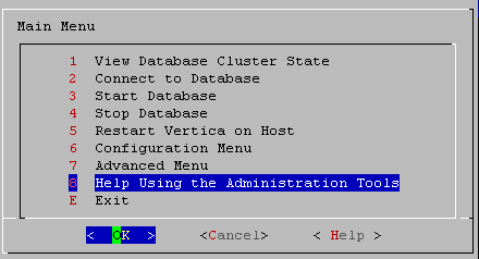
If you are unfamiliar with this type of interface, read Using the administration tools interface.
Privileges
dbadmin user
5.2 - First login as database administrator
The first time you log in as the and run the Administration Tools, the user interface displays.
The first time you log in as the Database Superuser and run the Administration Tools, the user interface displays.
-
In the end-user license agreement (EULA ) window, type accept to proceed.
A window displays, requesting the location of the license key file you downloaded from the Vertica website. The default path is
/tmp/vlicense.dat.
-
Type the absolute path to your license key (for example,
5.3 - Using the administration tools interface
The Vertica Administration Tools are implemented using Dialog, a graphical user interface that works in terminal (character-cell) windows.The interface responds to mouse clicks in some terminal windows, particularly local Linux windows, but you might find that it responds only to keystrokes.
The Vertica Administration Tools are implemented using Dialog, a graphical user interface that works in terminal (character-cell) windows.The interface responds to mouse clicks in some terminal windows, particularly local Linux windows, but you might find that it responds only to keystrokes. Thus, this section describes how to use the Administration Tools using only keystrokes.
Note
This section does not describe every possible combination of keystrokes you can use to accomplish a particular task. Feel free to experiment and to use whatever keystrokes you prefer.
Enter [return]
In all dialogs, when you are ready to run a command, select a file, or cancel the dialog, press the Enter key. The command descriptions in this section do not explicitly instruct you to press Enter.
OK - cancel - help
|
The OK, Cancel, and Help buttons are present on virtually all dialogs. Use the tab, space bar, or right and left arrow keys to select an option and then press Enter. The same keystrokes apply to dialogs that present a choice of Yes or No. |
|
|
Some dialogs require that you choose one command from a menu. Type the alphanumeric character shown or use the up and down arrow keys to select a command and then press Enter. |
 |
List dialogs
|
In a list dialog, use the up and down arrow keys to highlight items, then use the space bar to select the items (which marks them with an X). Some list dialogs allow you to select multiple items. When you have finished selecting items, press Enter. |
|
In a form dialog (also referred to as a dialog box), use the tab key to cycle between OK, Cancel, Help, and the form field area. Once the cursor is in the form field area, use the up and down arrow keys to select an individual field (highlighted) and enter information. When you have finished entering information in all fields, press Enter.
Online help is provided in the form of text dialogs. If you have trouble viewing the help, see Notes for remote terminal users.
5.4 - Notes for remote terminal users
The appearance of the graphical interface depends on the color and font settings used by your terminal window.
The appearance of the graphical interface depends on the color and font settings used by your terminal window. The screen captures in this document were made using the default color and font settings in a PuTTy terminal application running on a Windows platform.
Note
If you are using a remote terminal application, such as PuTTy or a Cygwin bash shell, make sure your window is at least 81 characters wide and 23 characters high.
If you are using PuTTY, you can make the Administration Tools look like the screen captures in this document:
-
In a PuTTY window, right click the title area and select Change Settings.
-
Create or load a saved session.
-
In the Category dialog, click Window > Appearance.
-
In the Font settings, click the Change... button.
-
Select Font: Courier New: Regular Size: 10
-
Click Apply.
Repeat these steps for each existing session that you use to run the Administration Tools.
You can also change the translation to support UTF-8:
-
In a PuTTY window, right click the title area and select Change Settings.
-
Create or load a saved session.
-
In the Category dialog, click Window > Translation.
-
In the "Received data assumed to be in which character set" drop-down menu, select UTF-8.
-
Click Apply.
5.5 - Using administration tools help
The Help on Using the Administration Tools command displays a help screen about using the Administration Tools.
The Help on Using the Administration Tools command displays a help screen about using the Administration Tools.
Most of the online help in the Administration Tools is context-sensitive. For example, if you use up/down arrows to select a command, press tab to move to the Help button, and press return, you get help on the selected command.
-
Use the up and down arrow keys to choose the command for which you want help.
-
Use the Tab key to move the cursor to the Help button.
-
Press Enter (Return).
In a dialog box
-
Use the up and down arrow keys to choose the field on which you want help.
-
Use the Tab key to move the cursor to the Help button.
-
Press Enter (Return).
Some help files are too long for a single screen. Use the up and down arrow keys to scroll through the text.
5.6 - Distributing changes made to the administration tools metadata
Administration Tools-specific metadata for a failed node will fall out of synchronization with other cluster nodes if you make the following changes:.
Administration Tools-specific metadata for a failed node will fall out of synchronization with other cluster nodes if you make the following changes:
When you restore the node to the database cluster, you can use the Administration Tools to update the node with the latest Administration Tools metadata:
-
Log on to a host that contains the metadata you want to transfer and start the Administration Tools. (See Using the administration tools.)
-
On the Main Menu in the Administration Tools, select Configuration Menu and click OK.
-
On the Configuration Menu, select Distribute Config Files and click OK.
-
Select AdminTools Meta-Data.
The Administration Tools metadata is distributed to every host in the cluster.
-
Restart the database.
5.7 - Administration tools and Management Console
You can perform most database administration tasks using the Administration Tools, but you have the additional option of using the more visual and dynamic.
You can perform most database administration tasks using the Administration Tools, but you have the additional option of using the more visual and dynamic Management Console.
The following table compares the functionality available in both interfaces. Continue to use Administration Tools and the command line to perform actions not yet supported by Management Console.
|
Vertica Functionality |
Management Console |
Administration Tools |
|
Use a Web interface for the administration of Vertica |
Yes |
No |
|
Manage/monitor one or more databases and clusters through a UI |
Yes |
No |
|
Manage multiple databases on different clusters |
Yes |
Yes |
|
View database cluster state |
Yes |
Yes |
|
View multiple cluster states |
Yes |
No |
|
Connect to the database |
Yes |
Yes |
|
Start/stop an existing database |
Yes |
Yes |
|
Stop/restart Vertica on host |
Yes |
Yes |
|
Kill a Vertica process on host |
No |
Yes |
|
Create one or more databases |
Yes |
Yes |
|
View databases |
Yes |
Yes |
|
Remove a database from view |
Yes |
No |
|
Drop a database |
Yes |
Yes |
|
Create a physical schema design (Database Designer) |
Yes |
Yes |
|
Modify a physical schema design (Database Designer) |
Yes |
Yes |
|
Set the restart policy |
No |
Yes |
|
Roll back database to the Last Good Epoch |
No |
Yes |
|
Manage clusters (add, replace, remove hosts) |
Yes |
Yes |
|
Rebalance data across nodes in the database |
Yes |
Yes |
|
Configure database parameters dynamically |
Yes |
No |
|
View database activity in relation to physical resource usage |
Yes |
No |
|
View alerts and messages dynamically |
Yes |
No |
|
View current database size usage statistics |
Yes |
No |
|
View database size usage statistics over time |
Yes |
No |
|
Upload/upgrade a license file |
Yes |
Yes |
|
Warn users about license violation on login |
Yes |
Yes |
|
Create, edit, manage, and delete users/user information |
Yes |
No |
|
Use LDAP to authenticate users with company credentials |
Yes |
Yes |
|
Manage user access to MC through roles |
Yes |
No |
|
Map Management Console users to a Vertica database |
Yes |
No |
|
Enable and disable user access to MC and/or the database |
Yes |
No |
|
Audit user activity on database |
Yes |
No |
|
Hide features unavailable to a user through roles |
Yes |
No |
|
Generate new user (non-LDAP) passwords |
Yes |
No |
Management Console Provides some, but Not All of the Functionality Provided By the Administration Tools. MC Also Provides Functionality Not Available in the Administration Tools.
See also
5.8 - Administration tools reference
Administration Tools, or "admintools," uses the open-source vertica-python client to perform operations on the database.
Administration Tools, or "admintools," uses the open-source vertica-python client to perform operations on the database.
The follow sections explain in detail all the steps you can perform with Vertica Administration Tools:
5.8.1 - Viewing database cluster state
This tool shows the current state of the nodes in the database.
This tool shows the current state of the nodes in the database.
-
On the Main Menu, select View Database Cluster State, and click OK.
The normal state of a running database is ALL UP. The normal state of a stopped database is ALL DOWN.
-
If some hosts are UP and some DOWN, restart the specific host that is down using Restart Vertica on Host from the Administration Tools, or you can start the database as described in Starting and Stopping the Database (unless you have a known node failure and want to continue in that state.)
Nodes shown as INITIALIZING or RECOVERING indicate that Failure recovery is in progress.
Nodes in other states (such as NEEDS_CATCHUP) are transitional and can be ignored unless they persist.
See also
5.8.2 - Connecting to the database
This tool connects to a running with.
This tool connects to a running database with vsql. You can use the Administration Tools to connect to a database from any node within the database while logged in to any user account with access privileges. You cannot use the Administration Tools to connect from a host that is not a database node. To connect from other hosts, run vsql as described in Connecting from the command line.
-
On the Main Menu, click Connect to Database, and then click OK.
-
Supply the database password if asked:
Password:
When you create a new user with the CREATE USER command, you can configure the password or leave it empty. You cannot bypass the password if the user was created with a password configured. You can change a user's password using the ALTER USER command.
The Administration Tools connect to the database and transfer control to vsql.
Welcome to vsql, the Vertica Analytic Database interactive terminal.
Type:  \h or \? for help with vsql commands
       \g or terminate with semicolon to execute query
       \q to quit

=>
See Using vsql for more information.
Note
After entering your password, you may be prompted to change your password if it has expired. See
Configuring client authentication for details of password security.
See also
5.8.3 - Restarting Vertica on host
This tool restarts the Vertica process on one or more hosts in a running database.
This tool restarts the Vertica process on one or more hosts in a running database. Use this tool if the Vertica process stopped or was killed on the host.
-
To view the current state nodes in cluster, on the Main Menu, select View Database Cluster State.
-
Click OK to return to the Main Menu.
-
If one or more nodes are down, select Restart Vertica on Host, and click OK.
-
Select the database that contains the host that you want to restart, and click OK.
-
Select the one or more hosts to restart, and click OK.
-
Enter the database password.
-
Select View Database Cluster State again to verify all nodes are up.
5.8.4 - Configuration menu options
The Configuration Menu allows you to perform the following tasks:.
The Configuration Menu allows you to perform the following tasks:
5.8.4.1 - Creating a database
Use the procedures below to create either an Enterprise Mode or Eon Mode database with admintools.
Use the procedures below to create either an Enterprise Mode or Eon Mode database with admintools. To create a database with an in-browser wizard in Management Console, see Creating a database using MC.
Create an Enterprise Mode database
-
On the Configuration Menu, click Create Database. Click OK.
-
Select Enterprise Mode as your database mode.
-
Enter the name of the database and an optional comment. Click OK.
-
Enter a password. See Creating a database name and password for rules.
If you do not enter a password, you are prompted to confirm: Yes to enter a superuser password, No to create a database without one.
Caution
If you do not enter a password at this point, superuser password is set to empty. Unless the database is for evaluation or academic purposes, Vertica strongly recommends that you enter a superuser password.
-
If you entered a password, enter the password again.
-
Select the hosts to include in the database. The hosts in this list are the ones that were specified at installation time (
install_vertica -s).
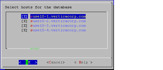
-
Specify the directories in which to store the catalog and data files.
Note
Catalog and data paths must contain only alphanumeric characters and cannot have leading space characters. Failure to comply with these restrictions could result in database creation failure.
Note
Do not use a shared directory for more than one node. Data and catalog directories must be distinct for each node. Multiple nodes must not be allowed to write to the same data or catalog directory.
-
Check the current database definition for correctness. Click Yes to proceed.
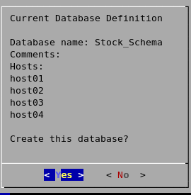
-
A message indicates that you have successfully created a database. Click OK.
Create an Eon Mode database
Note
Currently, the admintools menu interface does not support creating an Eon Mode database on Google Cloud Platform. Use the MC or the admintools command line to create an Eon Mode database instead.
-
On the Configuration Menu, click Create Database. Click OK.
-
Select Eon Mode as your database mode.
-
Enter the name of the database and an optional comment. Click OK.
-
Enter a password. See Creating a database name and password for rules.
AWS only: If you do not enter a password, you are prompted to confirm: Yes to enter a superuser password, No to create a database without one.
Caution
If you do not enter a password at this point, superuser password is set to empty. Unless the database is for evaluation or academic purposes, Vertica strongly recommends that you enter a superuser password.
-
If you entered a password, enter the password again.
-
Select the hosts to include in the database. The hosts in this list are those specified at installation time (
install_vertica -s).
-
Specify the directories in which to store the catalog and depot, depot size, communal storage location, and number of shards.
-
Depot Size: Use an integer followed by %, K, G, or T. Default is 60% of the disk total disk space of the filesystem storing the depot.
-
Communal Storage: Use an existing Amazon S3 bucket in the same region as your instances. Specify a new subfolder name, which Vertica will dynamically create within the existing S3 bucket. For example, s3://existingbucket/newstorage1. You can create a new subfolder within existing ones, but database creation will roll back if you do not specify any new subfolder name.
-
Number of Shards: Use a whole number. The default is equal to the number of nodes. For optimal performance, the number of shards should be no greater than 2x the number of nodes. When the number of nodes is greater than the number of shards (with ETS), the throughput of dashboard queries improves. When the number of shards exceeds the number of nodes, you can expand the cluster in the future to improve the performance of long analytic queries.
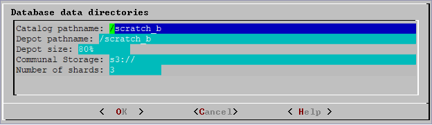
Note
Catalog and depot paths must contain only alphanumeric characters and cannot have leading space characters. Failure to comply with these restrictions could result in database creation failure.
-
Check the current database definition for correctness. Click Yes to proceed.
-
A message indicates that you successfully created a database. Click OK.
5.8.4.2 - Dropping a database
This tool drops an existing.
This tool drops an existing database. Only the Database Superuser is allowed to drop a database.
-
Stop the database.
-
On the Configuration Menu, click Drop Database and then click OK.
-
Select the database to drop and click OK.
-
Click Yes to confirm that you want to drop the database.
-
Type yes and click OK to reconfirm that you really want to drop the database.
-
A message indicates that you have successfully dropped the database. Click OK.
When Vertica drops the database, it also automatically drops the node definitions that refer to the database . The following exceptions apply:
-
Another database uses a node definition. If another database refers to any of these node definitions, none of the node definitions are dropped.
-
A node definition is the only node defined for the host. (Vertica uses node definitions to locate hosts that are available for database creation, so removing the only node defined for a host would make the host unavailable for new databases.)
5.8.4.3 - Viewing a database
This tool displays the characteristics of an existing .
This tool displays the characteristics of an existing database.
-
On the Configuration Menu, select View Database and click OK.
-
Select the database to view.
-
Vertica displays the following information about the database:
-
The name of the database.
-
The name and location of the log file for the database.
-
The hosts within the database cluster.
-
The value of the restart policy setting.
Note: This setting determines whether nodes within a K-Safe database are restarted when they are rebooted. See Setting the restart policy.
-
The database port.
-
The name and location of the catalog directory.
5.8.4.4 - Setting the restart policy
The Restart Policy enables you to determine whether or not nodes in a K-Safe are automatically restarted when they are rebooted.
The Restart Policy enables you to determine whether or not nodes in a K-Safe database are automatically restarted when they are rebooted. Since this feature does not automatically restart nodes if the entire database is DOWN, it is not useful for databases that are not K-Safe.
To set the Restart Policy for a database:
-
Open the Administration Tools.
-
On the Main Menu, select Configuration Menu, and click OK.
-
In the Configuration Menu, select Set Restart Policy, and click OK.
-
Select the database for which you want to set the Restart Policy, and click OK.
-
Select one of the following policies for the database:
-
Never — Nodes are never restarted automatically.
-
K-Safe — Nodes are automatically restarted if the database cluster is still UP. This is the default setting.
-
Always — Node on a single node database is restarted automatically.
Note
Always does not work if a single node database was not shutdown cleanly or crashed.
-
Click OK.
Best practice for restoring failed hardware
Following this procedure will prevent Vertica from misdiagnosing missing disk or bad mounts as data corruptions, which would result in a time-consuming, full-node recovery.
If a server fails due to hardware issues, for example a bad disk or a failed controller, upon repairing the hardware:
-
Reboot the machine into runlevel 1, which is a root and console-only mode.
Runlevel 1 prevents network connectivity and keeps Vertica from attempting to reconnect to the cluster.
-
In runlevel 1, validate that the hardware has been repaired, the controllers are online, and any RAID recover is able to proceed.
Note
You do not need to initialize RAID recover in runlevel 1; simply validate that it can recover.
-
Once the hardware is confirmed consistent, only then reboot to runlevel 3 or higher.
At this point, the network activates, and Vertica rejoins the cluster and automatically recovers any missing data. Note that, on a single-node database, if any files that were associated with a projection have been deleted or corrupted, Vertica will delete all files associated with that projection, which could result in data loss.
5.8.4.5 - Installing external procedure executable files
-
Run the Administration tools.
$ /opt/vertica/bin/adminTools
-
On the AdminTools Main Menu, click Configuration Menu, and then click OK.
-
On the Configuration Menu, click Install External Procedure and then click OK.
-
Select the database on which you want to install the external procedure.
-
Either select the file to install or manually type the complete file path, and then click OK.
-
If you are not the superuser, you are prompted to enter your password and click OK.
The Administration Tools automatically create the database-name/procedures directory on each node in the database and installs the external procedure in these directories for you.
-
Click OK in the dialog that indicates that the installation was successful.
5.8.5 - Advanced menu options
The Advanced Menu options allow you to perform the following tasks:.
The Advanced Menu options allow you to perform the following tasks:
5.8.5.1 - Rolling back the database to the last good epoch
Vertica provides the ability to roll the entire database back to a specific primarily to assist in the correction of human errors during data loads or other accidental corruptions.
Vertica provides the ability to roll the entire database back to a specific epoch primarily to assist in the correction of human errors during data loads or other accidental corruptions. For example, suppose that you have been performing a bulk load and the cluster went down during a particular COPY command. You might want to discard all epochs back to the point at which the previous COPY command committed and run the one that did not finish again. You can determine that point by examining the log files (see Monitoring the Log Files).
-
On the Advanced Menu, select Roll Back Database to Last Good Epoch.
-
Select the database to roll back. The database must be stopped.
-
Accept the suggested restart epoch or specify a different one.
-
Confirm that you want to discard the changes after the specified epoch.
The database restarts successfully.
Important
The default value of HistoryRetentionTime is 0, which means that Vertica only keeps historical data when nodes are down. This settings prevents the use of the Administration tools 'Roll Back Database to Last Good Epoch' option because the AHM remains close to the current epoch. Vertica cannot roll back to an epoch that precedes the AHM.
If you rely on the Roll Back option to remove recently loaded data, consider setting a day-wide window for removing loaded data. For example:
=> ALTER DATABASE DEFAULT SET HistoryRetentionTime = 86400;
5.8.5.2 - Stopping Vertica on host
This command attempts to gracefully shut down the Vertica process on a single node.
This command attempts to gracefully shut down the Vertica process on a single node.
Caution
Do not use this command to shut down the entire cluster. Instead,
stop the database to perform a clean shutdown that minimizes data loss.
-
On the Advanced Menu, select Stop Vertica on Host and click OK.
-
Select the hosts to stop.
-
Confirm that you want to stop the hosts.
If the command succeeds View Database Cluster State shows that the selected hosts are DOWN.
If the command fails to stop any selected nodes, proceed to Killing Vertica Process on Host.
5.8.5.3 - Killing the Vertica process on host
This command sends a kill signal to the Vertica process on a node.
This command sends a kill signal to the Vertica process on a node.
-
On the Advanced menu, select Kill Vertica Process on Host and click OK.
-
Select the hosts on which to kills the Vertica process.
-
Confirm that you want to stop the processes.
-
If the command succeeds, View Database Cluster State shows that the selected hosts are DOWN.
5.8.5.4 - Upgrading a Vertica license key
The following steps are for licensed Vertica users.
The following steps are for licensed Vertica users. Completing the steps copies a license key file into the database. See Managing licenses for more information.
-
On the Advanced menu select Upgrade License Key . Click OK.
-
Select the database for which to upgrade the license key.
-
Enter the absolute pathname of your downloaded license key file (for example,
/tmp/vlicense.dat). Click OK.
-
Click OK when you see a message indicating that the upgrade succeeded.
Note
If you are using Vertica Community Edition, follow the instructions in
Vertica license changes for instructions to upgrade to a Vertica Premium Edition license key.
5.8.5.5 - Managing clusters
Cluster Management lets you add, replace, or remove hosts from a database cluster.
Cluster Management lets you add, replace, or remove hosts from a database cluster. These processes are usually part of a larger process of adding, removing, or replacing a database node.
Using cluster management
To use Cluster Management:
-
From the Main Menu, select Advanced Menu, and then click OK.
-
In the Advanced Menu, select Cluster Management, and then click OK.
-
Select one of the following, and then click OK.
5.8.5.6 - Getting help on administration tools
The Help Using the Administration Tools command displays a help screen about using the Administration Tools.
The Help Using the Administration Tools command displays a help screen about using the Administration Tools.
Most of the online help in the Administration Tools is context-sensitive. For example, if you up the use up/down arrows to select a command, press tab to move to the Help button, and press return, you get help on the selected command.
5.8.5.7 - Administration tools metadata
The Administration Tools configuration data (metadata) contains information that databases need to start, such as the hostname/IP address of each participating host in the database cluster.
The Administration Tools configuration data (metadata) contains information that databases need to start, such as the hostname/IP address of each participating host in the database cluster.
To facilitate hostname resolution within the Administration Tools, at the command line, and inside the installation utility, Vertica enforces all hostnames you provide through the Administration Tools to use IP addresses:
-
During installation
Vertica immediately converts any hostname you provide through command line options --hosts, -add-hosts or --remove-hosts to its IP address equivalent.
-
If you provide a hostname during installation that resolves to multiple IP addresses (such as in multi-homed systems), the installer prompts you to choose one IP address.
-
Vertica retains the name you give for messages and prompts only; internally it stores these hostnames as IP addresses.
-
Within the Administration Tools
All hosts are in IP form to allow for direct comparisons (for example db = database = database.example.com).
-
At the command line
Vertica converts any hostname value to an IP address that it uses to look up the host in the configuration metadata. If a host has multiple IP addresses that are resolved, Vertica tests each IP address to see if it resides in the metadata, choosing the first match. No match indicates that the host is not part of the database cluster.
Metadata is more portable because Vertica does not require the names of the hosts in the cluster to be exactly the same when you install or upgrade your database.
5.8.6 - Administration tools connection behavior and requirements
The behavior of admintools when it connects to and performs operations on a database may vary based on your configuration.
The behavior of admintools when it connects to and performs operations on a database may vary based on your configuration. In particular, admintools considers its connection to other nodes, the status of those nodes, and the authentication method used by dbadmin.
Connection requirements and authentication
-
admintools uses passwordless SSH connections between cluster hosts for most operations, which is configured or confirmed during installation with the install_vertica script
-
For most situations, when issuing commands to the database, admintools prefers to uses its SSH connection to a target host and uses a localhost client connection to the Vertica database
-
The incoming IP address determines the authentication method used. That is, a client connection may have different behavior from a local connection, which may be trusted by default
-
dbadmin should have a local trust or password-based authentication method
-
When deciding which host to use for multi-step operations, admintools prefers localhost, and then to reconnect to known-to-be-good nodes
K-safety support
The Administration Tools allow certain operations on a K-Safe database, even if some nodes are unresponsive.
The database must have been marked as K-Safe using the MARK_DESIGN_KSAFE function.
The following management functions within the Administration Tools are operational when some nodes are unresponsive.
-
View database cluster state
-
Connect to database
-
Start database (including manual recovery)
-
Stop database
-
Replace node (assuming node that is down is the one being replaced)
-
View database parameters
-
Upgrade license key
The following management functions within the Administration Tools require that all nodes be UP in order to be operational:
5.8.7 - Writing administration tools scripts
You can invoke most Administration Tools from the command line or a shell script.
You can invoke most Administration Tools from the command line or a shell script.
Syntax
/opt/vertica/bin/admintools {
     { -h | --help }
   | { -a | --help_all}
   | { [--debug ] { -t | --tool } toolname [ tool-args ] }
}
Note
For convenience, add
/opt/vertica/bin to your search path.
Parameters
-h
-help |
Outputs abbreviated help. |
-a
-help_all |
Outputs verbose help, which lists all command-line sub-commands and options. |
[debug] { ‑t | ‑tool }toolname [args] |
Specifies the tool to run, where toolname is one of the tools listed in the help output described below, and args is one or more comma-delimited toolname arguments. If you include the debug option, Vertica logs debug information during tool execution. |
To return a list of all available tools, enter admintools -h at a command prompt.
To display help for a specific tool and its options or commands, qualify the specified tool name with --help or -h, as shown in the example below:
$ admintools -t connect_db --help
Usage: connect_db [options]

Options:
  -h, --help            show this help message and exit
  -d DB, --database=DB  Name of database to connect
  -p DBPASSWORD, --password=DBPASSWORD
                        Database password in single quotes
To list all available tools and their commands and options in individual help text, enter admintools -a.
Usage:
adminTools [-t | --tool] toolName [options]
Valid tools are:
command_host
connect_db
create_db
db_add_node
db_add_subcluster
db_remove_node
db_remove_subcluster
db_replace_node
db_status
distribute_config_files
drop_db
host_to_node
install_package
install_procedure
kill_host
kill_node
license_audit
list_allnodes
list_db
list_host
list_node
list_packages
logrotate
node_map
re_ip
rebalance_data
restart_db
restart_node
restart_subcluster
return_epoch
revive_db
set_restart_policy
set_ssl_params
show_active_db
start_db
stop_db
stop_host
stop_node
stop_subcluster
uninstall_package
upgrade_license_key
view_cluster
-------------------------------------------------------------------------
Usage: command_host [options]
Options:
-h, --help show this help message and exit
-c CMD, --command=CMD
Command to run
-F, --force Provide the force cleanup flag. Only applies to start,
restart, condrestart. For other options it is ignored.
-------------------------------------------------------------------------
Usage: connect_db [options]
Options:
-h, --help show this help message and exit
-d DB, --database=DB Name of database to connect
-p DBPASSWORD, --password=DBPASSWORD
Database password in single quotes
-------------------------------------------------------------------------
Usage: create_db [options]
Options:
-h, --help show this help message and exit
-D DATA, --data_path=DATA
Path of data directory[optional] if not using compat21
-c CATALOG, --catalog_path=CATALOG
Path of catalog directory[optional] if not using
compat21
--compat21 (deprecated) Use Vertica 2.1 method using node names
instead of hostnames
-d DB, --database=DB Name of database to be created
-l LICENSEFILE, --license=LICENSEFILE
Database license [optional]
-p DBPASSWORD, --password=DBPASSWORD
Database password in single quotes [optional]
-P POLICY, --policy=POLICY
Database restart policy [optional]
-s HOSTS, --hosts=HOSTS
comma-separated list of hosts to participate in
database
--shard-count=SHARD_COUNT
[Eon only] Number of shards in the database
--communal-storage-location=COMMUNAL_STORAGE_LOCATION
[Eon only] Location of communal storage
-x COMMUNAL_STORAGE_PARAMS, --communal-storage-params=COMMUNAL_STORAGE_PARAMS
[Eon only] Location of communal storage parameter file
--depot-path=DEPOT_PATH
[Eon only] Path to depot directory
--depot-size=DEPOT_SIZE
[Eon only] Size of depot
--force-cleanup-on-failure
Force removal of existing directories on failure of
command
--force-removal-at-creation
Force removal of existing directories before creating
the database
--timeout=NONINTERACTIVE_TIMEOUT
set a timeout (in seconds) to wait for actions to
complete ('never') will wait forever (implicitly sets
-i)
-i, --noprompts do not stop and wait for user input(default false).
Setting this implies a timeout of 20 min.
-------------------------------------------------------------------------
Usage: db_add_node [options]
Options:
-h, --help show this help message and exit
-d DB, --database=DB Name of the database
-s HOSTS, --hosts=HOSTS
Comma separated list of hosts to add to database
-p DBPASSWORD, --password=DBPASSWORD
Database password in single quotes
-a AHOSTS, --add=AHOSTS
Comma separated list of hosts to add to database
-c SCNAME, --subcluster=SCNAME
Name of subcluster for the new node
--timeout=NONINTERACTIVE_TIMEOUT
set a timeout (in seconds) to wait for actions to
complete ('never') will wait forever (implicitly sets
-i)
-i, --noprompts do not stop and wait for user input(default false).
Setting this implies a timeout of 20 min.
--compat21 (deprecated) Use Vertica 2.1 method using node names
instead of hostnames
-------------------------------------------------------------------------
Usage: db_add_subcluster [options]
Options:
-h, --help show this help message and exit
-d DB, --database=DB Name of database to be modified
-s HOSTS, --hosts=HOSTS
Comma separated list of hosts to add to the subcluster
-p DBPASSWORD, --password=DBPASSWORD
Database password in single quotes
-c SCNAME, --subcluster=SCNAME
Name of the new subcluster for the new node
--is-primary Create primary subcluster
--is-secondary Create secondary subcluster
--control-set-size=CONTROLSETSIZE
Set the number of nodes that will run spread within
the subcluster
--like=CLONESUBCLUSTER
Name of an existing subcluster from which to clone
properties for the new subcluster
--timeout=NONINTERACTIVE_TIMEOUT
set a timeout (in seconds) to wait for actions to
complete ('never') will wait forever (implicitly sets
-i)
-i, --noprompts do not stop and wait for user input(default false).
Setting this implies a timeout of 20 min.
-------------------------------------------------------------------------
Usage: db_remove_node [options]
Options:
-h, --help show this help message and exit
-d DB, --database=DB Name of database to be modified
-s HOSTS, --hosts=HOSTS
Name of the host to remove from the db
-p DBPASSWORD, --password=DBPASSWORD
Database password in single quotes
--timeout=NONINTERACTIVE_TIMEOUT
set a timeout (in seconds) to wait for actions to
complete ('never') will wait forever (implicitly sets
-i)
-i, --noprompts do not stop and wait for user input(default false).
Setting this implies a timeout of 20 min.
--compat21 (deprecated) Use Vertica 2.1 method using node names
instead of hostnames
--skip-directory-cleanup
Caution: this option will force you to do a manual
cleanup. This option skips directory deletion during
remove node. This is best used in a cloud environment
where the hosts being removed will be subsequently
discarded.
-------------------------------------------------------------------------
Usage: db_remove_subcluster [options]
Options:
-h, --help show this help message and exit
-d DB, --database=DB Name of database to be modified
-c SCNAME, --subcluster=SCNAME
Name of subcluster to be removed
-p DBPASSWORD, --password=DBPASSWORD
Database password in single quotes
--timeout=NONINTERACTIVE_TIMEOUT
set a timeout (in seconds) to wait for actions to
complete ('never') will wait forever (implicitly sets
-i)
-i, --noprompts do not stop and wait for user input(default false).
Setting this implies a timeout of 20 min.
--skip-directory-cleanup
Caution: this option will force you to do a manual
cleanup. This option skips directory deletion during
remove subcluster. This is best used in a cloud
environment where the hosts being removed will be
subsequently discarded.
-------------------------------------------------------------------------
Usage: db_replace_node [options]
Options:
-h, --help show this help message and exit
-d DB, --database=DB Name of the database
-o ORIGINAL, --original=ORIGINAL
Name of host you wish to replace
-n NEWHOST, --new=NEWHOST
Name of the replacement host
-p DBPASSWORD, --password=DBPASSWORD
Database password in single quotes
--timeout=NONINTERACTIVE_TIMEOUT
set a timeout (in seconds) to wait for actions to
complete ('never') will wait forever (implicitly sets
-i)
-i, --noprompts do not stop and wait for user input(default false).
Setting this implies a timeout of 20 min.
-------------------------------------------------------------------------
Usage: db_status [options]
Options:
-h, --help show this help message and exit
-s STATUS, --status=STATUS
Database status UP,DOWN or ALL(list running dbs -
UP,list down dbs - DOWN list all dbs - ALL
-------------------------------------------------------------------------
Usage: distribute_config_files
Sends admintools.conf from local host to all other hosts in the cluster
Options:
-h, --help show this help message and exit
-------------------------------------------------------------------------
Usage: drop_db [options]
Options:
-h, --help show this help message and exit
-d DB, --database=DB Database to be dropped
-------------------------------------------------------------------------
Usage: host_to_node [options]
Options:
-h, --help show this help message and exit
-s HOST, --host=HOST comma separated list of hostnames which is to be
converted into its corresponding nodenames
-d DB, --database=DB show only node/host mapping for this database.
-------------------------------------------------------------------------
Usage: admintools -t install_package --package PACKAGE -d DB -p PASSWORD
Examples:
admintools -t install_package -d mydb -p 'mypasswd' --package default
# (above) install all default packages that aren't currently installed
admintools -t install_package -d mydb -p 'mypasswd' --package default --force-reinstall
# (above) upgrade (re-install) all default packages to the current version
admintools -t install_package -d mydb -p 'mypasswd' --package hcat
# (above) install package hcat
See also: admintools -t list_packages
Options:
-h, --help show this help message and exit
-d DBNAME, --dbname=DBNAME
database name
-p PASSWORD, --password=PASSWORD
database admin password
-P PACKAGE, --package=PACKAGE
specify package or 'all' or 'default'
--force-reinstall Force a package to be re-installed even if it is
already installed.
-------------------------------------------------------------------------
Usage: install_procedure [options]
Options:
-h, --help show this help message and exit
-d DBNAME, --database=DBNAME
Name of database for installed procedure
-f PROCPATH, --file=PROCPATH
Path of procedure file to install
-p OWNERPASSWORD, --password=OWNERPASSWORD
Password of procedure file owner
-------------------------------------------------------------------------
Usage: kill_host [options]
Options:
-h, --help show this help message and exit
-s HOSTS, --hosts=HOSTS
comma-separated list of hosts on which the vertica
process is to be killed using a SIGKILL signal
--compat21 (deprecated) Use Vertica 2.1 method using node names
instead of hostnames
-------------------------------------------------------------------------
Usage: kill_node [options]
Options:
-h, --help show this help message and exit
-s HOSTS, --hosts=HOSTS
comma-separated list of hosts on which the vertica
process is to be killed using a SIGKILL signal
--compat21 (deprecated) Use Vertica 2.1 method using node names
instead of hostnames
-------------------------------------------------------------------------
Usage: license_audit --dbname DB_NAME [OPTIONS]
Runs audit and collects audit results.
Options:
-h, --help show this help message and exit
-d DATABASE, --database=DATABASE
Name of the database to retrieve audit results
-p PASSWORD, --password=PASSWORD
Password for database admin
-q, --quiet Do not print status messages.
-f FILE, --file=FILE Output results to FILE.
-------------------------------------------------------------------------
Usage: list_allnodes [options]
Options:
-h, --help show this help message and exit
-------------------------------------------------------------------------
Usage: list_db [options]
Options:
-h, --help show this help message and exit
-d DB, --database=DB Name of database to be listed
-------------------------------------------------------------------------
Usage: list_host [options]
Options:
-h, --help show this help message and exit
-------------------------------------------------------------------------
Usage: list_node [options]
Options:
-h, --help show this help message and exit
-n NODENAME, --node=NODENAME
Name of the node to be listed
-------------------------------------------------------------------------
Usage: admintools -t list_packages [OPTIONS]
Examples:
admintools -t list_packages # lists all available packages
admintools -t list_packages --package all # lists all available packages
admintools -t list_packages --package default # list all packages installed by default
admintools -t list_packages -d mydb --password 'mypasswd' # list the status of all packages in mydb
Options:
-h, --help show this help message and exit
-d DBNAME, --dbname=DBNAME
database name
-p PASSWORD, --password=PASSWORD
database admin password
-P PACKAGE, --package=PACKAGE
specify package or 'all' or 'default'
-------------------------------------------------------------------------
Usage: logrotateconfig [options]
Options:
-h, --help show this help message and exit
-d DBNAME, --dbname=DBNAME
database name
-r ROTATION, --rotation=ROTATION
set how often the log is rotated.[
daily|weekly|monthly ]
-s MAXLOGSZ, --maxsize=MAXLOGSZ
set maximum log size before rotation is forced.
-k KEEP, --keep=KEEP set # of old logs to keep
-------------------------------------------------------------------------
Usage: node_map [options]
Options:
-h, --help show this help message and exit
-d DB, --database=DB List only data for this database.
-------------------------------------------------------------------------
Usage: re_ip [options]
Replaces the IP addresses of hosts and databases in a cluster, or changes the
control messaging mode/addresses of a database.
Options:
-h, --help show this help message and exit
-f MAPFILE, --file=MAPFILE
A text file with IP mapping information. If the -O
option is not used, the command replaces the IP
addresses of the hosts in the cluster and all
databases for those hosts. In this case, the format of
each line in MAPFILE is: [oldIPaddress newIPaddress]
or [oldIPaddress newIPaddress, newControlAddress,
newControlBroadcast]. If the former,
'newControlAddress' and 'newControlBroadcast' would
set to default values. Usage: $ admintools -t re_ip -f
<mapfile>
-O, --db-only Updates the control messaging addresses of a database.
Also used for error recovery (when re_ip encounters
some certain errors, a mapfile is auto-generated).
Format of each line in MAPFILE: [NodeName
AssociatedNodeIPaddress, newControlAddress,
newControlBrodcast]. 'NodeName' and
'AssociatedNodeIPaddress' must be consistent with
admintools.conf. Usage: $ admintools -t re_ip -f
<mapfile> -O -d <db_name>
-i, --noprompts System does not prompt for the validation of the new
settings before performing the re_ip operation. Prompting is on
by default.
-T, --point-to-point Sets the control messaging mode of a database to
point-to-point. Usage: $ admintools -t re_ip -d
<db_name> -T
-U, --broadcast Sets the control messaging mode of a database to
broadcast. Usage: $ admintools -t re_ip -d <db_name>
-U
-d DB, --database=DB Name of a database. Required with the following
options: -O, -T, -U.
-------------------------------------------------------------------------
Usage: rebalance_data [options]
Options:
-h, --help show this help message and exit
-d DBNAME, --dbname=DBNAME
database name
-k KSAFETY, --ksafety=KSAFETY
specify the new k value to use
-p PASSWORD, --password=PASSWORD
--script Don't re-balance the data, just provide a script for
later use.
-------------------------------------------------------------------------
Usage: restart_db [options]
Options:
-h, --help show this help message and exit
-d DB, --database=DB Name of database to be restarted
-e EPOCH, --epoch=EPOCH
Epoch at which the database is to be restarted. If
'last' is given as argument the db is restarted from
the last good epoch.
-p DBPASSWORD, --password=DBPASSWORD
Database password in single quotes
-k, --allow-fallback-keygen
Generate spread encryption key from Vertica. Use under
support guidance only.
--timeout=NONINTERACTIVE_TIMEOUT
set a timeout (in seconds) to wait for actions to
complete ('never') will wait forever (implicitly sets
-i)
-i, --noprompts do not stop and wait for user input(default false).
Setting this implies a timeout of 20 min.
-------------------------------------------------------------------------
Usage: restart_node [options]
Options:
-h, --help show this help message and exit
-s HOSTS, --hosts=HOSTS
comma-separated list of hosts to be restarted
-d DB, --database=DB Name of database whose node is to be restarted
-p DBPASSWORD, --password=DBPASSWORD
Database password in single quotes
--new-host-ips=NEWHOSTS
comma-separated list of new IPs for the hosts to be
restarted
--timeout=NONINTERACTIVE_TIMEOUT
set a timeout (in seconds) to wait for actions to
complete ('never') will wait forever (implicitly sets
-i)
-i, --noprompts do not stop and wait for user input(default false).
Setting this implies a timeout of 20 min.
-F, --force force the node to start and auto recover if necessary
--compat21 (deprecated) Use Vertica 2.1 method using node names
instead of hostnames
--waitfordown-timeout=WAITTIME
Seconds to wait until nodes to be restarted are down
-------------------------------------------------------------------------
Usage: restart_subcluster [options]
Options:
-h, --help show this help message and exit
-d DB, --database=DB Name of database whose subcluster is to be restarted
-c SCNAME, --subcluster=SCNAME
Name of subcluster to be restarted
-p DBPASSWORD, --password=DBPASSWORD
Database password in single quotes
-s NEWHOSTS, --hosts=NEWHOSTS
Comma separated list of new hosts to rebind to the
nodes
--timeout=NONINTERACTIVE_TIMEOUT
set a timeout (in seconds) to wait for actions to
complete ('never') will wait forever (implicitly sets
-i)
-i, --noprompts do not stop and wait for user input(default false).
Setting this implies a timeout of 20 min.
-F, --force Force the nodes in the subcluster to start and auto
recover if necessary
-------------------------------------------------------------------------
Usage: return_epoch [options]
Options:
-h, --help show this help message and exit
-d DB, --database=DB Name of database
-p PASSWORD, --password=PASSWORD
Database password in single quotes
-------------------------------------------------------------------------
Usage: revive_db [options]
Options:
-h, --help show this help message and exit
-s HOSTS, --hosts=HOSTS
comma-separated list of hosts to participate in
database
-n NODEHOST, --node-and-host=NODEHOST
pair of nodename-hostname values delimited by "|" eg:
"v_testdb_node0001|10.0.0.1"Note: Each node-host pair
has to be specified as a new argument
--communal-storage-location=COMMUNAL_STORAGE_LOCATION
Location of communal storage
-x COMMUNAL_STORAGE_PARAMS, --communal-storage-params=COMMUNAL_STORAGE_PARAMS
Location of communal storage parameter file
-d DBNAME, --database=DBNAME
Name of database to be revived
--force Force cleanup of existing catalog directory
--display-only Describe the database on communal storage, and exit
--strict-validation Print warnings instead of raising errors while
validating cluster_config.json
-------------------------------------------------------------------------
Usage: set_restart_policy [options]
Options:
-h, --help show this help message and exit
-d DB, --database=DB Name of database for which to set policy
-p POLICY, --policy=POLICY
Restart policy: ('never', 'ksafe', 'always')
-------------------------------------------------------------------------
Usage: set_ssl_params [options]
Options:
-h, --help show this help message and exit
-d DB, --database=DB Name of database whose parameters will be set
-k KEYFILE, --ssl-key-file=KEYFILE
Path to SSL private key file
-c CERTFILE, --ssl-cert-file=CERTFILE
Path to SSL certificate file
-a CAFILE, --ssl-ca-file=CAFILE
Path to SSL CA file
-p DBPASSWORD, --password=DBPASSWORD
Database password in single quotes
-------------------------------------------------------------------------
Usage: show_active_db [options]
Options:
-h, --help show this help message and exit
-------------------------------------------------------------------------
Usage: start_db [options]
Options:
-h, --help show this help message and exit
-d DB, --database=DB Name of database to be started
-p DBPASSWORD, --password=DBPASSWORD
Database password in single quotes
--timeout=NONINTERACTIVE_TIMEOUT
set a timeout (in seconds) to wait for actions to
complete ('never') will wait forever (implicitly sets
-i)
-i, --noprompts do not stop and wait for user input(default false).
Setting this implies a timeout of 20 min.
-F, --force force the database to start at an epoch before data
consistency problems were detected.
-U, --unsafe Start database unsafely, skipping recovery. Use under
support guidance only.
-k, --allow-fallback-keygen
Generate spread encryption key from Vertica. Use under
support guidance only.
-s HOSTS, --hosts=HOSTS
comma-separated list of hosts to be started
--fast Attempt fast startup on un-encrypted eon db. Fast
startup will use startup information from
cluster_config.json
-------------------------------------------------------------------------
Usage: stop_db [options]
Options:
-h, --help show this help message and exit
-d DB, --database=DB Name of database to be stopped
-p DBPASSWORD, --password=DBPASSWORD
Database password in single quotes
-F, --force Force the databases to shutdown, even if users are
connected.
-z, --if-no-users Only shutdown if no users are connected.
If any users are connected, exit with an error.
-n DRAIN_SECONDS, --drain-seconds=DRAIN_SECONDS
Eon db only: seconds to wait for user connections to close.
Default value is 60 seconds.
When the time expires, connections will be forcibly closed
and the db will shut down.
--timeout=NONINTERACTIVE_TIMEOUT
set a timeout (in seconds) to wait for actions to
complete ('never') will wait forever (implicitly sets
-i)
-i, --noprompts do not stop and wait for user input(default false).
Setting this implies a timeout of 20 min.
-------------------------------------------------------------------------
Usage: stop_host [options]
Options:
-h, --help show this help message and exit
-s HOSTS, --hosts=HOSTS
comma-separated list of hosts on which the vertica
process is to be killed using a SIGTERM signal
--compat21 (deprecated) Use Vertica 2.1 method using node names
instead of hostnames
-------------------------------------------------------------------------
Usage: stop_node [options]
Options:
-h, --help show this help message and exit
-s HOSTS, --hosts=HOSTS
comma-separated list of hosts on which the vertica
process is to be killed using a SIGTERM signal
--compat21 (deprecated) Use Vertica 2.1 method using node names
instead of hostnames
-------------------------------------------------------------------------
Usage: stop_subcluster [options]
Options:
-h, --help show this help message and exit
-d DB, --database=DB Name of database whose subcluster is to be stopped
-c SCNAME, --subcluster=SCNAME
Name of subcluster to be stopped
-p DBPASSWORD, --password=DBPASSWORD
Database password in single quotes
-n DRAIN_SECONDS, --drain-seconds=DRAIN_SECONDS
Seconds to wait for user connections to close.
Default value is 60 seconds.
When the time expires, connections will be forcibly closed
and the db will shut down.
-F, --force Force the subcluster to shutdown immediately,
even if users are connected.
--timeout=NONINTERACTIVE_TIMEOUT
set a timeout (in seconds) to wait for actions to
complete ('never') will wait forever (implicitly sets
-i)
-i, --noprompts do not stop and wait for user input(default false).
Setting this implies a timeout of 20 min.
-------------------------------------------------------------------------
Usage: uninstall_package [options]
Options:
-h, --help show this help message and exit
-d DBNAME, --dbname=DBNAME
database name
-p PASSWORD, --password=PASSWORD
database admin password
-P PACKAGE, --package=PACKAGE
specify package or 'all' or 'default'
-------------------------------------------------------------------------
Usage: upgrade_license_key --database mydb --license my_license.key
upgrade_license_key --install --license my_license.key
Updates the vertica license.
Without '--install', updates the license used by the database and
the admintools license cache.
With '--install', updates the license cache in admintools that
is used for creating new databases.
Options:
-h, --help show this help message and exit
-d DB, --database=DB Name of database. Cannot be used with --install.
-l LICENSE, --license=LICENSE
Required - path to the license.
-i, --install When option is included, command will only update the
admintools license cache. Cannot be used with
--database.
-p PASSWORD, --password=PASSWORD
Database password.
-------------------------------------------------------------------------
Usage: view_cluster [options]
Options:
-h, --help show this help message and exit
-x, --xpand show the full cluster state, node by node
-d DB, --database=DB filter the output for a single database
6 - Operating the database
This topic explains how to start and stop your Vertica database, and how to use the database index tool.
This topic explains how to start and stop your Vertica database, and how to use the database index tool.
6.1 - Starting the database
You can start a database through one of the following:.
You can start a database through one of the following:
You can start a database with the Vertica Administration Tools:
-
Open the Administration Tools and select View Database Cluster State to make sure all nodes are down and no other database is running.
-
Open the Administration Tools. See Using the administration tools for information about accessing the Administration Tools.
-
On the Main Menu, select Start Database,and then select OK.
-
Select the database to start, and then click OK.
Caution
Start only one database at a time. If you start more than one database at a given time, results can be unpredictable: users are liable to encounter resource conflicts, or perform operations on the wrong database.
-
Enter the database password and click OK.
-
When prompted that the database started successfully, click OK.
-
Check the log files to make sure that no startup problems occurred.
Command line
You can start a database with the command line tool start_db:
$ /opt/vertica/bin/admintools ‑t start_db ‑d db‑name
     [‑p password]
     [‑s host1[,...] | ‑‑hosts=host1[,...]]
     [‑‑timeout seconds]
     [‑i | ‑‑noprompts]
     [‑‑fast]
     [‑F | ‑‑force]
|
Option |
Description |
‑d ‑‑database |
Name of database to start. |
‑p ‑‑password |
Required only during database creation, when you install a new license.
If the license is valid, the option ‑p (or ‑‑password) is not required to start the database and is silently ignored. This is by design, as the database can only be started by the user who (as part of the verticadba UNIX user group) initially created the database or who has root or su privileges.
If the license is invalid, Vertica uses the ‑p password argument to attempt to upgrade the license with the license file stored in /opt/vertica/config/share/license.key.
|
‑s ‑‑hosts |
(Eon Mode only) Comma delimited list of primary node host names or IP addresses. If you use this option, start_db attempts to start the database using just the nodes in the list. If omitted, start_db starts all database nodes.
For details, see Start Just the Primary Nodes in an Eon Mode Database below.
|
‑‑timeout |
The number of seconds a timeout in seconds to await startup completion. If set to never, start_db never times out (implicitly sets ‑i) |
‑i
‑‑noprompts |
Startup does not pause to await user input. Setting ‑i implies a timeout of 1200 seconds. |
‑‑fast |
(Eon Mode only) Attempts fast startup on an unencrypted database, using startup information from cluster_config.json. |
‑F
‑‑force |
Forces the database to start at an epoch before data consistency problems were detected. |
The following example uses start_db to start a single-node database:
$ /opt/vertica/bin/admintools -t start_db -d VMart
Info:
no password specified, using none
Node Status: v_vmart_node0001: (DOWN)
Node Status: v_vmart_node0001: (DOWN)
Node Status: v_vmart_node0001: (DOWN)
Node Status: v_vmart_node0001: (DOWN)
Node Status: v_vmart_node0001: (DOWN)
Node Status: v_vmart_node0001: (DOWN)
Node Status: v_vmart_node0001: (DOWN)
Node Status: v_vmart_node0001: (DOWN)
Node Status: v_vmart_node0001: (UP)
Database VMart started successfully
Eon Mode database node startup
On starting an Eon Mode database, you can start all primary nodes, or a subset of them. In both cases, pass start_db the list of the primary nodes to start with the ‑s option.
The following requirements apply:
- Primary node hosts must already be up to start the database.
- The
start_db tool cannot start stopped hosts such as cloud-based VMs. You must either manually start the hosts or use the MC to start the cluster.
The following example starts the three primary nodes in a six-node Eon Mode database:
$ admintools -t start_db -d verticadb -p 'password' \
   -s 10.11.12.10,10.11.12.20,10.11.12.30
    Starting nodes:
        v_verticadb_node0001 (10.11.12.10)
        v_verticadb_node0002 (10.11.12.20)
        v_verticadb_node0003 (10.11.12.30)
    Starting Vertica on all nodes. Please wait, databases with a large catalog may take a while to initialize.
    Node Status: v_verticadb_node0001: (DOWN) v_verticadb_node0002: (DOWN) v_verticadb_node0003: (DOWN)
    Node Status: v_verticadb_node0001: (DOWN) v_verticadb_node0002: (DOWN) v_verticadb_node0003: (DOWN)
    Node Status: v_verticadb_node0001: (DOWN) v_verticadb_node0002: (DOWN) v_verticadb_node0003: (DOWN)
    Node Status: v_verticadb_node0001: (DOWN) v_verticadb_node0002: (DOWN) v_verticadb_node0003: (DOWN)
    Node Status: v_verticadb_node0001: (DOWN) v_verticadb_node0002: (DOWN) v_verticadb_node0003: (DOWN)
    Node Status: v_verticadb_node0001: (DOWN) v_verticadb_node0002: (DOWN) v_verticadb_node0003: (DOWN)
    Node Status: v_verticadb_node0001: (UP) v_verticadb_node0002: (UP) v_verticadb_node0003: (UP)
Syncing catalog on verticadb with 2000 attempts.
Database verticadb: Startup Succeeded.  All Nodes are UP
After the database starts, the secondary subclusters are down. You can choose to start them as needed. See Starting a Subcluster.
Starting the database with a subset of primary nodes
As a best pratice, Vertica recommends that you always start an Eon Mode database with all primary nodes. Occasionally, you might be unable to start the hosts for all primary nodes. In that case, you might need to start the database with a subset of its primary nodes.
If start_db specifies a subset of database primary nodes, the following requirements apply:
- The nodes must comprise a quorum: at least 50% + 1 of all primary nodes in the cluster.
- Collectively, the nodes must provide coverage for all shards in communal storage. The primary nodes you use to start the database do not attempt to rebalance shard subscriptions while starting up.
If either or both of these conditions are not met, start_db returns an error. In the following example, start_db specifies three primary nodes in a database with nine primary nodes. The command returns an error that it cannot start the database with fewer than five primary nodes:
$ admintools -t start_db -d verticadb -p 'password' \
    -s 10.11.12.10,10.11.12.20,10.11.12.30
    Starting nodes:
        v_verticadb_node0001 (10.11.12.10)
        v_verticadb_node0002 (10.11.12.20)
        v_verticadb_node0003 (10.11.12.30)
Error: Quorum not satisfied for verticadb.
    3 < minimum 5  of 9 primary nodes.
Attempted to start the following nodes:
Primary
        v_verticadb_node0001 (10.11.12.10)
        v_verticadb_node0003 (10.11.12.30)
        v_verticadb_node0002 (10.11.12.20)
Secondary

 hint: you may want to start all primary nodes in the database
Database start up failed.  Cluster partitioned.
If you try to start the database with fewer than the full set of primary nodes and the cluster fails to start, Vertica processes might continue to run on some of the hosts. If so, subsequent attempts to start the database will return with an error like this:
Error: the vertica process for the database is running on the following hosts:
10.11.12.10
10.11.12.20
10.11.12.30
This may be because the process has not completed previous shutdown activities. Please wait and retry again.
Database start up failed.  Processes still running.
Database verticadb did not start successfully: Processes still running.. Hint: you may need to start all primary nodes.
Before you can start the database, you must stop the Vertica server process on the hosts listed in the error message, either with the admintools menus or the admintools command line's stop_host tool:
$ admintools -t stop_host -s 10.11.12.10,10.11.12.20,10.11.12.30
6.2 - Stopping the database
There are many occasions when you must stop a database, for example, before an upgrade or performing various maintenance tasks.
There are many occasions when you must stop a database, for example, before an upgrade or performing various maintenance tasks. You can stop a running database through one of the following:
You cannot stop a running database if any users are connected or Database Designer is building or deploying a database design.
To stop a running database with admintools:
-
Verify that all cluster nodes are up. If any nodes are down, identify and restart them.
-
Close all user sessions:
-
Identify all users with active sessions by querying the
SESSIONS system table. Notify users of the impending shutdown and request them to shut down their sessions.
-
Prevent users from starting new sessions by temporarily resetting configuration parameter MaxClientSessions to 0:
=> ALTER DATABASE DEFAULT SET MaxClientSessions = 0;
-
Close all remaining user sessions with Vertica functions CLOSE_SESSION and CLOSE_ALL_SESSIONS.
Note
You can also force a database shutdown and block new sessions with the function
SHUTDOWN.
-
Open Vertica Administration Tools.
-
From the Main Menu:
-
Select Stop Database
-
Click OK
-
Select the database to stop and click OK.
-
Enter the password (if asked) and click OK.
-
When prompted that database shutdown is complete, click OK.
Vertica functions
You can stop a database with the SHUTDOWN function. By default, the shutdown fails if any users are connected. To force a shutdown regardless of active user connections, call SHUTDOWN with an argument of true:
=> SELECT SHUTDOWN('true');
      SHUTDOWN
-------------------------
Shutdown: sync complete
(1 row)
In Eon Mode databases, you can stop subclusters with the SHUTDOWN_SUBCLUSTER and SHUTDOWN_WITH_DRAIN functions. SHUTDOWN_SUBCLUSTER shuts down subclusters immediately, whereas SHUTDOWN_WITH_DRAIN performs a graceful shutdown that drains client connections from subclusters before shutting them down. For more information, see Starting and stopping subclusters.
The following example demonstrates how you can shut down all subclusters in an Eon Mode database using SHUTDOWN_WITH_DRAIN:
=> SELECT SHUTDOWN_WITH_DRAIN('', 0);
NOTICE 0: Begin shutdown of subcluster (default_subcluster, analytics)
SHUTDOWN_WITH_DRAIN
-----------------------------------------------------------------------
Shutdown message sent to subcluster (default_subcluster, analytics)
(1 row)
Command line
You can stop a database with the admintools command stop_db:
$ $ admintools -t stop_db --help
Usage: stop_db [options]
Options:
-h, --help Show this help message and exit.
-d DB, --database=DB Name of database to be stopped.
-p DBPASSWORD, --password=DBPASSWORD
Database password in single quotes.
-F, --force Force the database to shutdown, even if users are
connected.
-z, --if-no-users Only shutdown if no users are connected. If any users
are connected, exit with an error.
-n DRAIN_SECONDS, --drain-seconds=DRAIN_SECONDS
Eon db only: seconds to wait for user connections to
close. Default value is 60 seconds. When the time
expires, connections will be forcibly closed and the
db will shut down.
--timeout=NONINTERACTIVE_TIMEOUT
Set a timeout (in seconds) to wait for actions to
complete ('never') will wait forever (implicitly sets
-i).
-i, --noprompts Do not stop and wait for user input(default false).
Setting this implies a timeout of 20 min.
Note
You cannot use both the -z (--if-no-users) and -F (or --force) options in the same stop_db call.
stop_db behavior depends on whether it stops an Eon Mode or Enterprise Mode database.
Stopping an Eon Mode database
In Eon Mode databases, the default behavior of stop_db is to call SHUTDOWN_WITH_DRAIN to gracefully shut down all subclusters in the database. This graceful shutdown process drains client connections from subclusters before shutting them down.
The stop_db option -n (--drain-seconds) lets you specify the number of seconds to wait—by default, 60—before forcefully closing client connections and shutting down all subclusters. If you set a negative -n value, the subclusters are marked as draining but do not shut down until all active user sessions disconnect.
In the following example, the database initially has an active client session, but the session closes before the timeout limit is reached and the database shuts down:
$ admintools -t stop_db -d verticadb --password password --drain-seconds 200
Shutdown will use connection draining.
Shutdown will wait for all client sessions to complete, up to 200 seconds
Then it will force a shutdown.
Poller has been running for 0:00:00.000025 seconds since 2022-07-27 17:10:08.292919
------------------------------------------------------------
client_sessions |node_count |node_names
--------------------------------------------------------------
0 |5 |v_verticadb_node0005,v_verticadb_node0006,v_verticadb_node0003,v_verticadb_node0...
1 |1 |v_verticadb_node0001
STATUS: vertica.engine.api.db_client.module is still running on 1 host: nodeIP as of 2022-07-27 17:10:18. See /opt/vertica/log/adminTools.log for full details.
Poller has been running for 0:00:11.371296 seconds since 2022-07-27 17:10:08.292919
...
------------------------------------------------------------
client_sessions |node_count |node_names
--------------------------------------------------------------
0 |5 |v_verticadb_node0002,v_verticadb_node0004,v_verticadb_node0003,v_verticadb_node0...
1 |1 |v_verticadb_node0001
Stopping poller drain_status because it was canceled
Shutdown metafunction complete. Polling until database processes have stopped.
Database verticadb stopped successfully
If you use the -z (--if-no-users) option, the database shuts down immediately if there are no active user sessions. Otherwise, the stop_db command returns an error:
$ admintools -t stop_db -d verticadb --password password --if-no-users
Running shutdown metafunction. Not using connection draining
Active session details
| Session id | Host Ip | Connected User |
| ------- -- | ---- -- | --------- ---- |
| v_verticadb_node0001-107720:0x257 | 192.168.111.31 | analyst |
Database verticadb not stopped successfully for the following reason:
Shutdown did not complete. Message: Shutdown: aborting shutdown
Active sessions prevented shutdown.
Omit the option --if-no-users to close sessions. See stop_db --help.
You can use the -F (or --force) option to shut down all subclusters immediately, without checking for active user sessions or draining the subclusters.
Stopping an Enterprise Mode database
In Enterprise Mode databases, the default behavior of stop_db is to shut down the database only if there are no active sessions. If users are connected to the database, the command aborts with an error message and lists all active sessions. For example:
$ /opt/vertica/bin/admintools -t stop_db -d VMart
Info: no password specified, using none
Active session details
| Session id | Host Ip | Connected User |
| ------- -- | ---- -- | --------- ---- |
| v_vmart_node0001-91901:0x162 | 10.20.100.247 | analyst |
Database VMart not stopped successfully for the following reason:
Unexpected output from shutdown: Shutdown: aborting shutdown
NOTICE: Cannot shut down while users are connected
You can use the -F (or --force) option to override user connections and force a shutdown.
6.3 - CRC and sort order check
As a superuser, you can run the Index tool on a Vertica database to perform two tasks:.
As a superuser, you can run the Index tool on a Vertica database to perform two tasks:
If the database is down, invoke the Index tool from the Linux command line. If the database is up, invoke from VSQL with Vertica meta-function
RUN_INDEX_TOOL:
|
Operation |
Database down |
Database up |
|
Run CRC |
/opt/vertica/bin/vertica ‑D catalog‑path ‑v |
SELECT RUN_INDEX_TOOL ('checkcrc',... ); |
|
Check sort order |
/opt/vertica/bin/vertica ‑D catalog‑path ‑I |
SELECT RUN_INDEX_TOOL ('checksort',... ); |
If invoked from the command line, the Index tool runs only on the current node. However, you can run the Index tool on multiple nodes simultaneously.
Result output
The Index tool writes summary information about its operation to standard output; detailed information on results is logged in one of two locations, depending on the environment where you invoke the tool:
|
Invoked from: |
Results written to: |
|
Linux command line |
indextool.log in the database catalog directory |
|
VSQL |
vertica.log on the current node |
For information about evaluating output for possible errors, see:
You can optimize meta-function performance by narrowing the scope of the operation to one or more projections, and specifying the number of threads used to execute the function. For details, see
RUN_INDEX_TOOL.
6.3.1 - Evaluating CRC errors
Vertica evaluates the CRC values in each ROS data block each time it fetches data disk to process a query.
Vertica evaluates the CRC values in each ROS data block each time it fetches data disk to process a query. If CRC errors occur while fetching data, the following information is written to the vertica.log file:
CRC Check Failure Details:File Name:
File Offset:
Compressed size in file:
Memory Address of Read Buffer:
Pointer to Compressed Data:
Memory Contents:
The Event Manager is also notified of CRC errors, so you can use an SNMP trap to capture CRC errors:
"CRC mismatch detected on file <file_path>. File may be corrupted. Please check hardware and drivers."
If you run a query from vsql, ODBC, or JDBC, the query returns a FileColumnReader ERROR. This message indicates that a specific block's CRC does not match a given record as follows:
hint: Data file may be corrupt. Ensure that all hardware (disk and memory) is working properly.
Possible solutions are to delete the file <pathname> while the node is down, and then allow the node
to recover, or truncate the table data.code: ERRCODE_DATA_CORRUPTED
6.3.2 - Evaluating sort order errors
If ROS data is not sorted correctly in the projection's order, query results that rely on sorted data will be incorrect.
If ROS data is not sorted correctly in the projection's order, query results that rely on sorted data will be incorrect. You can use the Index tool to check the ROS sort order if you suspect or detect incorrect query results. The Index tool evaluates each ROS row to determine whether it is sorted correctly. If the check locates a row that is not in order, it writes an error message to the log file with the row number and contents of the unsorted row.
Reviewing errors
-
Open the indextool.log file. For example:
$ cd VMart/v_check_node0001_catalog
-
Look for error messages that include an OID number and the string Sort Order Violation. For example:
<INFO> ...on oid 45035996273723545: Sort Order Violation:
-
Find detailed information about the sort order violation string by running grep on indextool.log. For example, the following command returns the line before each string (-B1), and the four lines that follow (-A4):
[15:07:55][vertica-s1]: grep -B1 -A4 'Sort Order Violation:' /my_host/databases/check/v_check_node0001_catalog/indextool.log
2012-06-14 14:07:13.686 unknown:0x7fe1da7a1950 [EE] <INFO> An error occurred when running index tool thread on oid 45035996273723537:
Sort Order Violation:
Row Position: 624
Column Index: 0
Last Row: 2576000
This Row: 2575000
--
2012-06-14 14:07:13.687 unknown:0x7fe1dafa2950 [EE] <INFO> An error occurred when running index tool thread on oid 45035996273723545:
Sort Order Violation:
Row Position: 3
Column Index: 0
Last Row: 4
This Row: 2
--
-
Find the projection where a sort order violation occurred by querying system table
STORAGE_CONTAINERS. Use a storage_oid equal to the OID value listed in indextool.log. For example:
=> SELECT * FROM storage_containers WHERE storage_oid = 45035996273723545;
7 - Working with native tables
You can create two types of native tables in Vertica (ROS format), columnar and flexible.
You can create two types of native tables in Vertica (ROS format), columnar and flexible. You can create both types as persistent or temporary. You can also create views that query a specific set of table columns.
The tables described in this section store their data in and are managed by the Vertica database. Vertica also supports external tables, which are defined in the database and store their data externally. For more information about external tables, see Working with external data.
7.1 - Creating tables
Use the CREATE TABLE statement to create a native table in the Vertica.
Use the CREATE TABLE statement to create a native table in the Vertica logical schema. You can specify the columns directly, as in the following example, or you can derive a table definition from another table using a LIKE or AS clause. You can specify constraints, partitioning, segmentation, and other factors. For details and restrictions, see the reference page.
The following example shows a basic table definition:
=> CREATE TABLE orders(
orderkey INT,
custkey INT,
prodkey ARRAY[VARCHAR(10)],
orderprices ARRAY[DECIMAL(12,2)],
orderdate DATE
);
Table data storage
Unlike traditional databases that store data in tables, Vertica physically stores table data in projections, which are collections of table columns. Projections store data in a format that optimizes query execution. Similar to materialized views, they store result sets on disk rather than compute them each time they are used in a query.
In order to query or perform any operation on a Vertica table, the table must have one or more projections associated with it. For more information, see Projections.
Deriving a table definition from the data
You can use the INFER_TABLE_DDL function to inspect Parquet, ORC, JSON, or Avro data and produce a starting point for a table definition. This function returns a CREATE TABLE statement, which might require further editing. For columns where the function could not infer the data type, the function labels the type as unknown and emits a warning. For VARCHAR and VARBINARY columns, you might need to adjust the length. Always review the statement the function returns, but especially for tables with many columns, using this function can save time and effort.
Parquet, ORC, and Avro files include schema information, but JSON files do not. For JSON, the function inspects the raw data to produce one or more candidate table definitions. See the function reference page for JSON examples.
In the following example, the function infers a complete table definition from Parquet input, but the VARCHAR columns use the default size and might need to be adjusted:
=> SELECT INFER_TABLE_DDL('/data/people/*.parquet'
USING PARAMETERS format = 'parquet', table_name = 'employees');
WARNING 9311: This generated statement contains one or more varchar/varbinary columns which default to length 80
INFER_TABLE_DDL
-------------------------------------------------------------------------
create table "employees"(
"employeeID" int,
"personal" Row(
"name" varchar,
"address" Row(
"street" varchar,
"city" varchar,
"zipcode" int
),
"taxID" int
),
"department" varchar
);
(1 row)
For Parquet files, you can use the GET_METADATA function to inspect a file and report metadata including information about columns.
See also
7.2 - Creating temporary tables
CREATE TEMPORARY TABLE creates a table whose data persists only during the current session.
CREATE TEMPORARY TABLE creates a table whose data persists only during the current session. Temporary table data is never visible to other sessions.
By default, all temporary table data is transaction-scoped—that is, the data is discarded when a COMMIT statement ends the current transaction. If CREATE TEMPORARY TABLE includes the parameter ON COMMIT PRESERVE ROWS, table data is retained until the current session ends.
Temporary tables can be used to divide complex query processing into multiple steps. Typically, a reporting tool holds intermediate results while reports are generated—for example, the tool first gets a result set, then queries the result set, and so on.
When you create a temporary table, Vertica automatically generates a default projection for it. For more information, see Auto-projections.
Global versus local tables
CREATE TEMPORARY TABLE can create tables at two scopes, global and local, through the keywords GLOBAL and LOCAL, respectively:
|
Global temporary tables |
Vertica creates global temporary tables in the public schema. Definitions of these tables are visible to all sessions, and persist across sessions until they are explicitly dropped. Multiple users can access the table concurrently. Table data is session-scoped, so it is visible only to the session user, and is discarded when the session ends. |
|
Local temporary tables |
Vertica creates local temporary tables in the V_TEMP_SCHEMA namespace and inserts them transparently into the user's search path. These tables are visible only to the session where they are created. When the session ends, Vertica automatically drops the table and its data. |
Data retention
You can specify whether temporary table data is transaction- or session-scoped:
Note
If you create a temporary table with ON COMMIT PRESERVE ROWS, you cannot add projections for that table if it contains data. You must first remove all data from that table with
TRUNCATE TABLE.
You can create projections for temporary tables created with ON COMMIT DELETE ROWS, whether populated with data or not. However, CREATE PROJECTION ends any transaction where you might have added data, so projections are always empty.
ON COMMIT DELETE ROWS
By default, Vertica removes all data from a temporary table, whether global or local, when the current transaction ends.
For example:
=> CREATE TEMPORARY TABLE tempDelete (a int, b int);
CREATE TABLE
=> INSERT INTO tempDelete VALUES(1,2);
OUTPUT
--------
1
(1 row)
=> SELECT * FROM tempDelete;
a | b
---+---
1 | 2
(1 row)
=> COMMIT;
COMMIT
=> SELECT * FROM tempDelete;
a | b
---+---
(0 rows)
If desired, you can use
DELETE within the same transaction multiple times, in order to refresh table data repeatedly.
ON COMMIT PRESERVE ROWS
You can specify that a temporary table retain data across transactions in the current session, by defining the table with the keywords ON COMMIT PRESERVE ROWS. Vertica automatically removes all data from the table only when the current session ends.
For example:
=> CREATE TEMPORARY TABLE tempPreserve (a int, b int) ON COMMIT PRESERVE ROWS;
CREATE TABLE
=> INSERT INTO tempPreserve VALUES (1,2);
OUTPUT
--------
1
(1 row)
=> COMMIT;
COMMIT
=> SELECT * FROM tempPreserve;
a | b
---+---
1 | 2
(1 row)
=> INSERT INTO tempPreserve VALUES (3,4);
OUTPUT
--------
1
(1 row)
=> COMMIT;
COMMIT
=> SELECT * FROM tempPreserve;
a | b
---+---
1 | 2
3 | 4
(2 rows)
Eon restrictions
The following Eon Mode restrictions apply to temporary tables:
7.3 - Creating a table from other tables
You can create a table from other tables in two ways:.
You can create a table from other tables in two ways:
Important
You can also copy one table to another with the Vertica function
COPY_TABLE.
7.3.1 - Replicating a table
You can create a table from an existing one using CREATE TABLE with the LIKE clause:.
You can create a table from an existing one using
CREATE TABLE with the LIKE clause:
CREATE TABLE [schema.]table-name LIKE [schema.]existing-table
[ {INCLUDING | EXCLUDING} PROJECTIONS ]
[ {INCLUDE | EXCLUDE} [SCHEMA] PRIVILEGES ]
Creating a table with LIKE replicates the source table definition and any storage policy associated with it. It does not copy table data or expressions on columns.
Copying constraints
CREATE TABLE...LIKE copies all table constraints, with the following exceptions:
-
Foreign key constraints.
-
Any column that obtains its values from a sequence, including IDENTITY columns. Vertica copies the column values into the new table, but removes the original constraint. For example, the following table definition sets an IDENTITY constraint on column ID:
CREATE TABLE public.Premium_Customer
(
ID IDENTITY ,
lname varchar(25),
fname varchar(25),
store_membership_card int
);
The following CREATE TABLE...LIKE statement replicates this table as All_Customers. Vertica removes the IDENTITY constraint from All_Customers.ID, changing it to an integer column with a NOT NULL constraint:
=> CREATE TABLE All_Customers like Premium_Customer;
CREATE TABLE
=> select export_tables('','All_Customers');
export_tables
---------------------------------------------------
CREATE TABLE public.All_Customers
(
ID int NOT NULL,
lname varchar(25),
fname varchar(25),
store_membership_card int
);
(1 row)
Including projections
You can qualify the LIKE clause with INCLUDING PROJECTIONS or EXCLUDING PROJECTIONS, which specify whether to copy projections from the source table:
-
EXCLUDING PROJECTIONS (default): Do not copy projections from the source table.
-
INCLUDING PROJECTIONS: Copy current projections from the source table. Vertica names the new projections according to Vertica naming conventions, to avoid name conflicts with existing objects.
Including schema privileges
You can specify default inheritance of schema privileges for the new table:
For more information see Setting privilege inheritance on tables and views.
Restrictions
The following restrictions apply to the source table:
Example
-
Create the table states:
=> CREATE TABLE states (
state char(2) NOT NULL, bird varchar(20), tree varchar (20), tax float, stateDate char (20))
PARTITION BY state;
-
Populate the table with data:
INSERT INTO states VALUES ('MA', 'chickadee', 'american_elm', 5.675, '07-04-1620');
INSERT INTO states VALUES ('VT', 'Hermit_Thrasher', 'Sugar_Maple', 6.0, '07-04-1610');
INSERT INTO states VALUES ('NH', 'Purple_Finch', 'White_Birch', 0, '07-04-1615');
INSERT INTO states VALUES ('ME', 'Black_Cap_Chickadee', 'Pine_Tree', 5, '07-04-1615');
INSERT INTO states VALUES ('CT', 'American_Robin', 'White_Oak', 6.35, '07-04-1618');
INSERT INTO states VALUES ('RI', 'Rhode_Island_Red', 'Red_Maple', 5, '07-04-1619');
-
View the table contents:
=> SELECT * FROM states;
state | bird | tree | tax | stateDate
-------+---------------------+--------------+-------+----------------------
VT | Hermit_Thrasher | Sugar_Maple | 6 | 07-04-1610
CT | American_Robin | White_Oak | 6.35 | 07-04-1618
RI | Rhode_Island_Red | Red_Maple | 5 | 07-04-1619
MA | chickadee | american_elm | 5.675 | 07-04-1620
NH | Purple_Finch | White_Birch | 0 | 07-04-1615
ME | Black_Cap_Chickadee | Pine_Tree | 5 | 07-04-1615
(6 rows
-
Create a sample projection and refresh:
=> CREATE PROJECTION states_p AS SELECT state FROM states;
=> SELECT START_REFRESH();
-
Create a table like the states table and include its projections:
=> CREATE TABLE newstates LIKE states INCLUDING PROJECTIONS;
-
View projections for the two tables. Vertica has copied projections from states to newstates:
=> \dj
List of projections
Schema | Name | Owner | Node | Comment
-------------------------------+-------------------------------------------+---------+------------------+---------
public | newstates_b0 | dbadmin | |
public | newstates_b1 | dbadmin | |
public | newstates_p_b0 | dbadmin | |
public | newstates_p_b1 | dbadmin | |
public | states_b0 | dbadmin | |
public | states_b1 | dbadmin | |
public | states_p_b0 | dbadmin | |
public | states_p_b1 | dbadmin | |
-
View the table newstates, which shows columns copied from states:
=> SELECT * FROM newstates;
state | bird | tree | tax | stateDate
-------+------+------+-----+-----------
(0 rows)
When you use the CREATE TABLE...LIKE statement, storage policy objects associated with the table are also copied. Data added to the new table use the same labeled storage location as the source table, unless you change the storage policy. For more information, see Working With Storage Locations.
See also
7.3.2 - Creating a table from a query
CREATE TABLE can specify an AS clause to create a table from a query, as follows:.
CREATE TABLE can specify an AS clause to create a table from a query, as follows:
CREATE [TEMPORARY] TABLE [schema.]table-name
[ ( column-name-list ) ]
[ {INCLUDE | EXCLUDE} [SCHEMA] PRIVILEGES ]
AS [ /*+ LABEL */ ] [ AT epoch ] query [ ENCODED BY column‑ref‑list ]
Vertica creates a table from the query results and loads the result set into it. For example:
=> CREATE TABLE cust_basic_profile AS SELECT
customer_key, customer_gender, customer_age, marital_status, annual_income, occupation
FROM customer_dimension WHERE customer_age>18 AND customer_gender !='';
CREATE TABLE
=> SELECT customer_age, annual_income, occupation FROM cust_basic_profile
WHERE customer_age > 23 ORDER BY customer_age;
customer_age | annual_income | occupation
--------------+---------------+--------------------
24 | 469210 | Hairdresser
24 | 140833 | Butler
24 | 558867 | Lumberjack
24 | 529117 | Mechanic
24 | 322062 | Acrobat
24 | 213734 | Writer
...
AS clause options
You can qualify an AS clause with one or both of the following options:
Labeling the AS clause
You can embed a LABEL hint in an AS clause in two places:
-
Immediately after the keyword AS:
CREATE TABLE myTable AS /*+LABEL myLabel*/...
-
In the SELECT statement:
CREATE TABLE myTable AS SELECT /*+LABEL myLabel*/
If the AS clause contains a LABEL hint in both places, the first label has precedence.
Note
Labels are invalid for external tables.
Loading historical data
You can qualify a CREATE TABLE AS query with an AT epoch clause, to specify that the query return historical data, where epoch is one of the following:
-
EPOCH LATEST: Return data up to but not including the current epoch. The result set includes data from the latest committed DML transaction.
-
EPOCH integer: Return data up to and including the integer-specified epoch.
-
TIME 'timestamp': Return data from the timestamp-specified epoch.
Note
These options are ignored if used to query temporary or external tables.
See Epochs for additional information about how Vertica uses epochs.
For details, see Historical queries.
Zero-width column handling
If the query returns a column with zero width, Vertica automatically converts it to a VARCHAR(80) column. For example:
Note
=> CREATE TABLE example AS SELECT '' AS X;
CREATE TABLE
=> SELECT EXPORT_TABLES ('', 'example');
EXPORT_TABLES
----------------------------------------------------------
CREATE TEMPORARY TABLE public.example
(
X varchar(80)
);
Requirements and restrictions
-
If you create a temporary table from a query, you must specify ON COMMIT PRESERVE ROWS in order to load the result set into the table. Otherwise, Vertica creates an empty table.
-
If the query output has expressions other than simple columns, such as constants or functions, you must specify an alias for that expression, or list all columns in the column name list.
-
You cannot use CREATE TABLE AS SELECT with a SELECT that returns values of complex types. You can, however, use CREATE TABLE LIKE.
See also
7.4 - Immutable tables
Many secure systems contain records that must be provably immune to change.
Many secure systems contain records that must be provably immune to change. Protective strategies such as row and block checksums incur high overhead. Moreover, these approaches are not foolproof against unauthorized changes, whether deliberate or inadvertent, by database administrators or other users with sufficient privileges.
Immutable tables are insert-only tables in which existing data cannot be modified, regardless of user privileges. Updating row values and deleting rows are prohibited. Certain changes to table metadata—for example, renaming table columns—are also prohibited, in order to prevent attempts to circumvent these restrictions. Flattened or external tables, which obtain their data from outside sources, cannot be set to be immutable.
You define an existing table as immutable with ALTER TABLE:
ALTER TABLE table SET IMMUTABLE ROWS;
Once set, table immutability cannot be reverted, and is immediately applied to all existing table data, and all data that is loaded thereafter. In order to modify the data of an immutable table, you must copy the data to a new table—for example, with COPY, CREATE TABLE...AS, or COPY_TABLE.
When you execute ALTER TABLE...SET IMMUTABLE ROWS on a table, Vertica sets two columns for that table in the system table TABLES. Together, these columns show when the table was made immutable:
- immutable_rows_since_timestamp: Server system time when immutability was applied. This is valuable for long-term timestamp retrieval and efficient comparison.
- immutable_rows_since_epoch: The epoch that was current when immutability was applied. This setting can help protect the table from attempts to pre-insert records with a future timestamp, so that row's epoch is less than the table's immutability epoch.
Enforcement
The following operations are prohibited on immutable tables:
The following partition management functions are disallowed when the target table is immutable:
Allowed operations
In general, you can execute any DML operation on an immutable table that does not affect existing row data—for example, add rows with COPY or INSERT. After you add data to an immutable table, it cannot be changed.
Tip
A table's immutability can render meaningless certain operations that are otherwise permitted on an immutable table. For example, you can add a column to an immutable table with
ALTER TABLE...ADD COLUMN. However, all values in the new column are set to NULL (unless the column is defined with a
DEFAULT value), and they cannot be updated.
Other allowed operations fall generally into two categories:
-
Changes to a table's DDL that have no effect on its data:
-
Block operations on multiple table rows, or the entire table:
7.5 - Disk quotas
By default, schemas and tables are limited only by available disk space and license capacity.
By default, schemas and tables are limited only by available disk space and license capacity. You can set disk quotas for schemas or individual tables, for example, to support multi-tenancy. Setting, modifying, or removing a disk quota requires superuser privileges.
Most user operations that increase storage size enforce disk quotas. A table can temporarily exceed its quota during some operations such as recovery. If you lower a quota below the current usage, no data is lost but you cannot add more. Treat quotas as advisory, not as hard limits
A schema quota, if set, must be larger than the largest table quota within it.
A disk quota is a string composed of an integer and a unit of measure (K, M, G, or T), such as '15G' or '1T'. Do not use a space between the number and the unit. No other units of measure are supported.
To set a quota at creation time, use the DISK_QUOTA option for CREATE SCHEMA or CREATE TABLE:
=> CREATE SCHEMA internal DISK_QUOTA '10T';
CREATE SCHEMA
=> CREATE TABLE internal.sales (...) DISK_QUOTA '5T';
CREATE TABLE
=> CREATE TABLE internal.leads (...) DISK_QUOTA '12T';
ROLLBACK 0: Table can not have a greater disk quota than its Schema
To modify, add, or remove a quota on an existing schema or table, use ALTER SCHEMA or ALTER TABLE:
=> ALTER SCHEMA internal DISK_QUOTA '20T';
ALTER SCHEMA
=> ALTER TABLE internal.sales DISK_QUOTA SET NULL;
ALTER TABLE
You can set a quota that is lower than the current usage. The ALTER operation succeeds, the schema or table is temporarily over quota, and you cannot perform operations that increase data usage.
Data that is counted
In Eon Mode, disk usage is an aggregate of all space used by all shards for the schema or table. This value is computed for primary subscriptions only.
In Enterprise Mode, disk usage is the sum space used by all storage containers on all nodes for the schema or table. This sum excludes buddy projections but includes all other projections.
Disk usage is calculated based on compressed size.
When quotas are applied
Quotas, if present, affect most DML and ILM operations, including:
The following example shows a failure caused by exceeding a table's quota:
=> CREATE TABLE stats(score int) DISK_QUOTA '1k';
CREATE TABLE
=> COPY stats FROM STDIN;
1
2
3
4
5
\.
ERROR 0: Disk Quota Exceeded for the Table object public.stats
HINT: Delete data and PURGE or increase disk quota at the table level
DELETE does not free space, because deleted data is still preserved in the storage containers. The delete vector that is added by a delete operation does not count against a quota, so deleting is a quota-neutral operation. Disk space for deleted data is reclaimed when you purge it; see Removing table data.
Some uncommon operations, such as ADD COLUMN, RESTORE, and SWAP PARTITION, can create new storage containers during the transaction. These operations clean up the extra locations upon completion, but while the operation is in progress, a table or schema could exceed its quota. If you get disk-quota errors during these operations, you can temporarily increase the quota, perform the operation, and then reset it.
Quotas do not affect recovery, rebalancing, or Tuple Mover operations.
Monitoring
The DISK_QUOTA_USAGES system table shows current disk usage for tables and schemas that have quotas. This table does not report on objects that do not have quotas.
You can use this table to monitor usage and make decisions about adjusting quotas:
=> SELECT * FROM DISK_QUOTA_USAGES;
object_oid | object_name | is_schema | total_disk_usage_in_bytes | disk_quota_in_bytes
-------------------+-------------+-----------+---------------------+---------------------
45035996273705100 | s | t | 307 | 10240
45035996273705104 | public.t | f | 614 | 1024
45035996273705108 | s.t | f | 307 | 2048
(3 rows)
7.6 - Managing table columns
After you define a table, you can use ALTER TABLE to modify existing table columns.
After you define a table, you can use
ALTER TABLE to modify existing table columns. You can perform the following operations on a column:
7.6.1 - Renaming columns
You rename a column with ALTER TABLE as follows:.
You rename a column with ALTER TABLE as follows:
ALTER TABLE [schema.]table-name RENAME [ COLUMN ] column-name TO new-column-name
The following example renames a column in the Retail.Product_Dimension table from Product_description to Item_description:
=> ALTER TABLE Retail.Product_Dimension
RENAME COLUMN Product_description TO Item_description;
If you rename a column that is referenced by a view, the column does not appear in the result set of the view even if the view uses the wild card (*) to represent all columns in the table. Recreate the view to incorporate the column's new name.
7.6.2 - Changing scalar column data type
In general, you can change a column's data type with ALTER TABLE if doing so does not require storage reorganization.
In general, you can change a column's data type with ALTER TABLE if doing so does not require storage reorganization. After you modify a column's data type, data that you load conforms to the new definition.
The sections that follow describe requirements and restrictions associated with changing a column with a scalar (primitive) data type. For information on modifying complex type columns, see Adding a new field to a complex type column.
Supported data type conversions
Vertica supports conversion for the following data types:
|
Data Types |
Supported Conversions |
|
Binary |
Expansion and contraction. |
|
Character |
All conversions between CHAR, VARCHAR, and LONG VARCHAR. |
|
Exact numeric |
All conversions between the following numeric data types: integer data types—INTEGER, INT, BIGINT, TINYINT, INT8, SMALLINT—and NUMERIC values of scale <=18 and precision 0.
You cannot modify the scale of NUMERIC data types; however, you can change precision in the ranges (0-18), (19-37), and so on.
|
|
Collection |
The following conversions are supported:
- Collection of one element type to collection of another element type, if the source element type can be coerced to the target element type.
- Between arrays and sets.
- Collection type to the same type (array to array or set to set), to change bounds or binary size.
For details, see Changing Collection Columns.
|
Unsupported data type conversions
Vertica does not allow data type conversion on types that require storage reorganization:
You also cannot change a column's data type if the column is one of the following:
You can work around some of these restrictions. For details, see Working with column data conversions.
7.6.2.1 - Changing column width
You can expand columns within the same class of data type.
You can expand columns within the same class of data type. Doing so is useful for storing larger items in a column. Vertica validates the data before it performs the conversion.
In general, you can also reduce column widths within the data type class. This is useful to reclaim storage if the original declaration was longer than you need, particularly with strings. You can reduce column width only if the following conditions are true:
Otherwise, Vertica returns an error and the conversion fails. For example, if you try to convert a column from varchar(25) to varchar(10)Vertica allows the conversion as long as all column data is no more than 10 characters.
In the following example, columns y and z are initially defined as VARCHAR data types, and loaded with values 12345 and 654321, respectively. The attempt to reduce column z's width to 5 fails because it contains six-character data. The attempt to reduce column y's width to 5 succeeds because its content conforms with the new width:
=> CREATE TABLE t (x int, y VARCHAR, z VARCHAR);
CREATE TABLE
=> CREATE PROJECTION t_p1 AS SELECT * FROM t SEGMENTED BY hash(x) ALL NODES;
CREATE PROJECTION
=> INSERT INTO t values(1,'12345','654321');
OUTPUT
--------
1
(1 row)
=> SELECT * FROM t;
x | y | z
---+-------+--------
1 | 12345 | 654321
(1 row)
=> ALTER TABLE t ALTER COLUMN z SET DATA TYPE char(5);
ROLLBACK 2378: Cannot convert column "z" to type "char(5)"
HINT: Verify that the data in the column conforms to the new type
=> ALTER TABLE t ALTER COLUMN y SET DATA TYPE char(5);
ALTER TABLE
Changing collection columns
If a column is a collection data type, you can use ALTER TABLE to change either its bounds or its maximum binary size. These properties are set at table creation time and can then be altered.
You can make a collection bounded, setting its maximum number of elements, as in the following example.
=> ALTER TABLE test.t1 ALTER COLUMN arr SET DATA TYPE array[int,10];
ALTER TABLE
=> \d test.t1
List of Fields by Tables
Schema | Table | Column | Type | Size | Default | Not Null | Primary Key | Foreign Key
--------+-------+--------+-----------------+------+---------+----------+-------------+-------------
test | t1 | arr | array[int8, 10] | 80 | | f | f |
(1 row)
Alternatively, you can set the binary size for the entire collection instead of setting bounds. Binary size is set either explicitly or from the DefaultArrayBinarySize configuration parameter. The following example creates an array column from the default, changes the default, and then uses ALTER TABLE to change it to the new default.
=> SELECT get_config_parameter('DefaultArrayBinarySize');
get_config_parameter
----------------------
100
(1 row)
=> CREATE TABLE test.t1 (arr array[int]);
CREATE TABLE
=> \d test.t1
List of Fields by Tables
Schema | Table | Column | Type | Size | Default | Not Null | Primary Key | Foreign Key
--------+-------+--------+-----------------+------+---------+----------+-------------+-------------
test | t1 | arr | array[int8](96) | 96 | | f | f |
(1 row)
=> ALTER DATABASE DEFAULT SET DefaultArrayBinarySize=200;
ALTER DATABASE
=> ALTER TABLE test.t1 ALTER COLUMN arr SET DATA TYPE array[int];
ALTER TABLE
=> \d test.t1
List of Fields by Tables
Schema | Table | Column | Type | Size | Default | Not Null | Primary Key | Foreign Key
--------+-------+--------+-----------------+------+---------+----------+-------------+-------------
test | t1 | arr | array[int8](200)| 200 | | f | f |
(1 row)
Alternatively, you can set the binary size explicitly instead of using the default value.
=> ALTER TABLE test.t1 ALTER COLUMN arr SET DATA TYPE array[int](300);
Purging historical data
You cannot reduce a column's width if Vertica retains any historical data that exceeds the new width. To reduce the column width, first remove that data from the table:
-
Advance the AHM to an epoch more recent than the historical data that needs to be removed from the table.
-
Purge the table of all historical data that precedes the AHM with the function
PURGE_TABLE.
For example, given the previous example, you can update the data in column t.z as follows:
=> UPDATE t SET z = '54321';
OUTPUT
--------
1
(1 row)
=> SELECT * FROM t;
x | y | z
---+-------+-------
1 | 12345 | 54321
(1 row)
Although no data in column z now exceeds 5 characters, Vertica retains the history of its earlier data, so attempts to reduce the column width to 5 return an error:
=> ALTER TABLE t ALTER COLUMN z SET DATA TYPE char(5);
ROLLBACK 2378: Cannot convert column "z" to type "char(5)"
HINT: Verify that the data in the column conforms to the new type
You can reduce the column width by purging the table's historical data as follows:
=> SELECT MAKE_AHM_NOW();
MAKE_AHM_NOW
-------------------------------
AHM set (New AHM Epoch: 6350)
(1 row)
=> SELECT PURGE_TABLE('t');
PURGE_TABLE
----------------------------------------------------------------------------------------------------------------------
Task: purge operation
(Table: public.t) (Projection: public.t_p1_b0)
(Table: public.t) (Projection: public.t_p1_b1)
(1 row)
=> ALTER TABLE t ALTER COLUMN z SET DATA TYPE char(5);
ALTER TABLE
7.6.2.2 - Working with column data conversions
Vertica conforms to the SQL standard by disallowing certain data conversions for table columns.
Vertica conforms to the SQL standard by disallowing certain data conversions for table columns. However, you sometimes need to work around this restriction when you convert data from a non-SQL database. The following examples describe one such workaround, using the following table:
=> CREATE TABLE sales(id INT, price VARCHAR) UNSEGMENTED ALL NODES;
CREATE TABLE
=> INSERT INTO sales VALUES (1, '$50.00');
OUTPUT
--------
1
(1 row)
=> INSERT INTO sales VALUES (2, '$100.00');
OUTPUT
--------
1
(1 row)
=> COMMIT;
COMMIT
=> SELECT * FROM SALES;
id | price
----+---------
1 | $50.00
2 | $100.00
(2 rows)
To convert the price column's existing data type from VARCHAR to NUMERIC, complete these steps:
-
Add a new column for temporary use. Assign the column a NUMERIC data type, and derive its default value from the existing price column.
-
Drop the original price column.
-
Rename the new column to the original column.
Add a new column for temporary use
-
Add a column temp_price to table sales. You can use the new column temporarily, setting its data type to what you want (NUMERIC), and deriving its default value from the price column. Cast the default value for the new column to a NUMERIC data type and query the table:
=> ALTER TABLE sales ADD COLUMN temp_price NUMERIC(10,2) DEFAULT
SUBSTR(sales.price, 2)::NUMERIC;
ALTER TABLE
=> SELECT * FROM SALES;
id | price | temp_price
----+---------+------------
1 | $50.00 | 50.00
2 | $100.00 | 100.00
(2 rows)
-
Use ALTER TABLE to drop the default expression from the new column temp_price. Vertica retains the values stored in this column:
=> ALTER TABLE sales ALTER COLUMN temp_price DROP DEFAULT;
ALTER TABLE
Drop the original price column
Drop the extraneous price column. Before doing so, you must first advance the AHM to purge historical data that would otherwise prevent the drop operation:
-
Advance the AHM:
=> SELECT MAKE_AHM_NOW();
MAKE_AHM_NOW
-------------------------------
AHM set (New AHM Epoch: 6354)
(1 row)
-
Drop the original price column:
=> ALTER TABLE sales DROP COLUMN price CASCADE;
ALTER COLUMN
Rename the new column to the original column
You can now rename the temp_price column to price:
-
Use ALTER TABLE to rename the column:
=> ALTER TABLE sales RENAME COLUMN temp_price to price;
-
Query the sales table again:
=> SELECT * FROM sales;
id | price
----+--------
1 | 50.00
2 | 100.00
(2 rows)
7.6.3 - Adding a new field to a complex type column
You can add new fields to columns of complex types (any combination or nesting of arrays and structs) in native tables.
You can add new fields to columns of complex types (any combination or nesting of arrays and structs) in native tables. To add a field to an existing table's column, use a single ALTER TABLE statement.
Requirements and restrictions
The following are requirements and restrictions associated with adding a new field to a complex type column:
- New fields can only be added to rows/structs.
- The new type definition must contain all of the existing fields in the complex type column. Dropping existing fields from the complex type is not allowed. All of the existing fields in the new type must exactly match their definitions in the old type.This requirement also means that existing fields cannot be renamed.
- New fields can only be added to columns of native (non-external) tables.
- New fields can be added at any level within a nested complex type. For example, if you have a column defined as
ROW(id INT, name ROW(given_name VARCHAR(20), family_name VARCHAR(20)), you can add a middle_name field to the nested ROW.
- New fields can be of any type, either complex or primitive.
- Blank field names are not allowed when adding new fields. Note that blank field names in complex type columns are allowed when creating the table. Vertica automatically assigns a name to each unnamed field.
- If you change the ordering of existing fields using ALTER TABLE, the change affects existing data in addition to new data. This means it is possible to reorder existing fields.
- When you call ALTER COLUMN ... SET DATA TYPE to add a field to a complex type column, Vertica will place an O lock on the table preventing DELETE, UPDATE, INSERT, and COPY statements from accessing the table and blocking SELECT statements issued at SERIALIZABLE isolation level, until the operation completes.
- Performance is slower when adding a field to an array element than when adding a field to an element not nested in an array.
Examples
Adding a field
Consider a company storing customer data:
=> CREATE TABLE customers(id INT, name VARCHAR, address ROW(street VARCHAR, city VARCHAR, zip INT));
CREATE TABLE
The company has just decided to expand internationally, so now needs to add a country field:
=> ALTER TABLE customers ALTER COLUMN address
SET DATA TYPE ROW(street VARCHAR, city VARCHAR, zip INT, country VARCHAR);
ALTER TABLE
You can view the table definition to confirm the change:
=> \d customers
List of Fields by Tables
Schema | Table | Column | Type | Size | Default | Not Null | Primary Key | Foreign Key
--------+-----------+---------+----------------------------------------------------------------------+------+---------+----------+-------------+-------------
public | customers | id | int | 8 | | f | f |
public | customers | name | varchar(80) | 80 | | f | f |
public | customers | address | ROW(street varchar(80),city varchar(80),zip int,country varchar(80)) | -1 | | f | f |
(3 rows)
You can also see that the country field remains null for existing customers:
=> SELECT * FROM customers;
id | name | address
----+------+--------------------------------------------------------------------------------
1 | mina | {"street":"1 allegheny square east","city":"hamden","zip":6518,"country":null}
(1 row)
Common error messages
While you can add one or more fields with a single ALTER TABLE statement, existing fields cannot be removed. The following example throws an error because the city field is missing:
=> ALTER TABLE customers ALTER COLUMN address SET DATA TYPE ROW(street VARCHAR, state VARCHAR, zip INT, country VARCHAR);
ROLLBACK 2377: Cannot convert column "address" from "ROW(varchar(80),varchar(80),int,varchar(80))" to type "ROW(varchar(80),varchar(80),int,varchar(80))"
Similarly, you cannot alter the type of an existing field. The following example will throw an error because the zip field's type cannot be altered:
=> ALTER TABLE customers ALTER COLUMN address SET DATA TYPE ROW(street VARCHAR, city VARCHAR, zip VARCHAR, country VARCHAR);
ROLLBACK 2377: Cannot convert column "address" from "ROW(varchar(80),varchar(80),int,varchar(80))" to type "ROW(varchar(80),varchar(80),varchar(80),varchar(80))"
Additional properties
A complex type column's field order follows the order specified in the ALTER command, allowing you to reorder a column's existing fields. The following example reorders the fields of the address column:
=> ALTER TABLE customers ALTER COLUMN address
SET DATA TYPE ROW(street VARCHAR, country VARCHAR, city VARCHAR, zip INT);
ALTER TABLE
The table definition shows the address column's fields have been reordered:
=> \d customers
List of Fields by Tables
Schema | Table | Column | Type | Size | Default | Not Null | Primary Key | Foreign Key
--------+-----------+---------+----------------------------------------------------------------------+------+---------+----------+-------------+-------------
public | customers | id | int | 8 | | f | f |
public | customers | name | varchar(80) | 80 | | f | f |
public | customers | address | ROW(street varchar(80),country varchar(80),city varchar(80),zip int) | -1 | | f | f |
(3 rows)
Note that you cannot add new fields with empty names. When creating a complex table, however, you can omit field names, and Vertica automatically assigns a name to each unnamed field:
=> CREATE TABLE products(name VARCHAR, description ROW(VARCHAR));
CREATE TABLE
Because the field created in the description column has not been named, Vertica assigns it a default name. This default name can be checked in the table definition:
=> \d products
List of Fields by Tables
Schema | Table | Column | Type | Size | Default | Not Null | Primary Key | Foreign Key
--------+----------+-------------+---------------------+------+---------+----------+-------------+-------------
public | products | name | varchar(80) | 80 | | f | f |
public | products | description | ROW(f0 varchar(80)) | -1 | | f | f |
(2 rows)
Above, we see that the VARCHAR field in the description column was automatically assigned the name f0. When adding new fields, you must specify the existing Vertica-assigned field name:
=> ALTER TABLE products ALTER COLUMN description
SET DATA TYPE ROW(f0 VARCHAR(80), expanded_description VARCHAR(200));
ALTER TABLE
7.6.4 - Defining column values
You can define a column so Vertica automatically sets its value from an expression through one of the following clauses:.
You can define a column so Vertica automatically sets its value from an expression through one of the following clauses:
-
DEFAULT
-
SET USING
-
DEFAULT USING
DEFAULT
The DEFAULT option sets column values to a specified value. It has the following syntax:
DEFAULT default-expression
Default values are set when you:
-
Load new rows into a table, for example, with INSERT or COPY. Vertica populates DEFAULT columns in new rows with their default values. Values in existing rows, including columns with DEFAULT expressions, remain unchanged.
-
Execute UPDATE on a table and set the value of a DEFAULT column to DEFAULT:
=> UPDATE table-name SET column-name=DEFAULT;
-
Add a column with a DEFAULT expression to an existing table. Vertica populates the new column with its default values when it is added to the table.
Note
Altering an existing table column to specify a DEFAULT expression has no effect on existing values in that column. Vertica applies the DEFAULT expression only on new rows when they are added to the table, through load operations such as INSERT and COPY. To refresh all values in a column with the column's DEFAULT expression, update the column as shown above.
Restrictions
DEFAULT expressions cannot specify volatile functions with ALTER TABLE...ADD COLUMN. To specify volatile functions, use CREATE TABLE or ALTER TABLE...ALTER COLUMN statements.
SET USING
The SET USING option sets the column value to an expression when the function REFRESH_COLUMNS is invoked on that column. This option has the following syntax:
SET USING using-expression
This approach is useful for large denormalized (flattened) tables, where multiple columns get their values by querying other tables.
Restrictions
SET USING has the following restrictions:
DEFAULT USING
The DEFAULT USING option sets DEFAULT and SET USING constraints on a column, equivalent to using DEFAULT and SET USING separately with the same expression on the same column. It has the following syntax:
DEFAULT USING expression
For example, the following column definitions are effectively identical:
=> ALTER TABLE public.orderFact ADD COLUMN cust_name varchar(20)
DEFAULT USING (SELECT name FROM public.custDim WHERE (custDim.cid = orderFact.cid));
=> ALTER TABLE public.orderFact ADD COLUMN cust_name varchar(20)
DEFAULT (SELECT name FROM public.custDim WHERE (custDim.cid = orderFact.cid))
SET USING (SELECT name FROM public.custDim WHERE (custDim.cid = orderFact.cid));
DEFAULT USING supports the same expressions as SET USING and is subject to the same restrictions.
Supported expressions
DEFAULT and SET USING generally support the same expressions. These include:
-
Queries
-
Other columns in the same table
-
Literals (constants)
-
All operators supported by Vertica
-
The following categories of functions:
Expression restrictions
The following restrictions apply to DEFAULT and SET USING expressions:
-
The return value data type must match or be cast to the column data type.
-
The expression must return a value that conforms to the column bounds. For example, a column that is defined as a VARCHAR(1) cannot be set to a default string of abc.
-
In a temporary table, DEFAULT and SET USING do not support subqueries. If you try to create a temporary table where DEFAULT or SET USING use subquery expressions, Vertica returns an error.
-
A column's SET USING expression cannot specify another column in the same table that also sets its value with SET USING. Similarly, a column's DEFAULT expression cannot specify another column in the same table that also sets its value with DEFAULT, or whose value is automatically set to a sequence. However, a column's SET USING expression can specify another column that sets its value with DEFAULT.
Note
You can set a column's DEFAULT expression from another column in the same table that sets its value with SET USING. However, the DEFAULT column is typically set to NULL, as it is only set on load operations that initially set the SET USING column to NULL.
-
DEFAULT and SET USING expressions only support one SELECT statement; attempts to include multiple SELECT statements in the expression return an error. For example, given table t1:
=> SELECT * FROM t1;
a | b
---+---------
1 | hello
2 | world
(2 rows)
Attempting to create table t2 with the following DEFAULT expression returns with an error:
=> CREATE TABLE t2 (aa int, bb varchar(30) DEFAULT (SELECT 'I said ')||(SELECT b FROM t1 where t1.a = t2.aa));
ERROR 9745: Expressions with multiple SELECT statements cannot be used in 'set using' query definitions
Disambiguating predicate columns
If a SET USING or DEFAULT query expression joins two columns with the same name, the column names must include their table names. Otherwise, Vertica assumes that both columns reference the dimension table, and the predicate always evaluates to true.
For example, tables orderFact and custDim both include column cid. Flattened table orderFact defines column cust_name with a SET USING query expression. Because the query predicate references columns cid from both tables, the column names are fully qualified:
=> CREATE TABLE public.orderFact
(
...
cid int REFERENCES public.custDim(cid),
cust_name varchar(20) SET USING (
SELECT name FROM public.custDim WHERE (custDIM.cid = orderFact.cid)),
...
)
Examples
Derive a column's default value from another column
-
Create table t with two columns, date and state, and insert a row of data:
=> CREATE TABLE t (date DATE, state VARCHAR(2));
CREATE TABLE
=> INSERT INTO t VALUES (CURRENT_DATE, 'MA');
OUTPUT
--------
1
(1 row)
=> COMMIT;
COMMMIT
SELECT * FROM t;
date | state
------------+-------
2017-12-28 | MA
(1 row)
-
Use ALTER TABLE to add a third column that extracts the integer month value from column date:
=> ALTER TABLE t ADD COLUMN month INTEGER DEFAULT date_part('month', date);
ALTER TABLE
-
When you query table t, Vertica returns the number of the month in column date:
=> SELECT * FROM t;
date | state | month
------------+-------+-------
2017-12-28 | MA | 12
(1 row)
Update default column values
-
Update table t by subtracting 30 days from date:
=> UPDATE t SET date = date-30;
OUTPUT
--------
1
(1 row)
=> COMMIT;
COMMIT
=> SELECT * FROM t;
date | state | month
------------+-------+-------
2017-11-28 | MA | 12
(1 row)
The value in month remains unchanged.
-
Refresh the default value in month from column date:
=> UPDATE t SET month=DEFAULT;
OUTPUT
--------
1
(1 row)
=> COMMIT;
COMMIT
=> SELECT * FROM t;
date | state | month
------------+-------+-------
2017-11-28 | MA | 11
(1 row)
Derive a default column value from user-defined scalar function
This example shows a user-defined scalar function that adds two integer values. The function is called add2ints and takes two arguments.
-
Develop and deploy the function, as described in Scalar functions (UDSFs).
-
Create a sample table, t1, with two integer columns:
=> CREATE TABLE t1 ( x int, y int );
CREATE TABLE
-
Insert some values into t1:
=> insert into t1 values (1,2);
OUTPUT
--------
1
(1 row)
=> insert into t1 values (3,4);
OUTPUT
--------
1
(1 row)
-
Use ALTER TABLE to add a column to t1, with the default column value derived from the UDSF add2ints:
alter table t1 add column z int default add2ints(x,y);
ALTER TABLE
-
List the new column:
select z from t1;
z
----
3
7
(2 rows)
Table with a SET USING column that queries another table for its values
-
Define tables t1 and t2. Column t2.b is defined to get its data from column t1.b, through the query in its SET USING clause:
=> CREATE TABLE t1 (a INT PRIMARY KEY ENABLED, b INT);
CREATE TABLE
=> CREATE TABLE t2 (a INT, alpha VARCHAR(10),
b INT SET USING (SELECT t1.b FROM t1 WHERE t1.a=t2.a))
ORDER BY a SEGMENTED BY HASH(a) ALL NODES;
CREATE TABLE
Important
The definition for table t2 includes SEGMENTED BY and ORDER BY clauses that exclude SET USING column b. If these clauses are omitted, Vertica creates an auto-projection for this table that specifies column b in its SEGMENTED BY and ORDER BY clauses . Inclusion of a SET USING column in any projection's segmentation or sort order prevents function REFRESH_COLUMNS from populating this column. Instead, it returns with an error.
For details on this and other restrictions, see REFRESH_COLUMNS.
-
Populate the tables with data:
=> INSERT INTO t1 VALUES(1,11),(2,22),(3,33),(4,44);
=> INSERT INTO t2 VALUES (1,'aa'),(2,'bb');
=> COMMIT;
COMMIT
-
View the data in table t2: Column in SET USING column b is empty, pending invocation of Vertica function REFRESH_COLUMNS:
=> SELECT * FROM t2;
a | alpha | b
---+-------+---
1 | aa |
2 | bb |
(2 rows)
-
Refresh the column data in table t2 by calling function REFRESH_COLUMNS:
=> SELECT REFRESH_COLUMNS ('t2','b', 'REBUILD');
REFRESH_COLUMNS
---------------------------
refresh_columns completed
(1 row)
In this example, REFRESH_COLUMNS is called with the optional argument REBUILD. This argument specifies to replace all data in SET USING column b. It is generally good practice to call REFRESH_COLUMNS with REBUILD on any new SET USING column. For details, see REFRESH_COLUMNS.
-
View data in refreshed column b, whose data is obtained from table t1 as specified in the column's SET USING query:
=> SELECT * FROM t2 ORDER BY a;
a | alpha | b
---+-------+----
1 | aa | 11
2 | bb | 22
(2 rows)
DEFAULT and SET USING expressions support subqueries that can obtain values from other tables, and use those with values in the current table to compute column values. The following example adds a column gmt_delivery_time to fact table customer_orders. The column specifies a DEFAULT expression to set values in the new column as follows:
-
Calls meta-function NEW_TIME, which performs the following tasks:
-
Populates the gmt_delivery_time column with the converted values.
=> CREATE TABLE public.customers(
customer_key int,
customer_name varchar(64),
customer_address varchar(64),
customer_tz varchar(5),
...);
=> CREATE TABLE public.customer_orders(
customer_key int,
order_number int,
product_key int,
product_version int,
quantity_ordered int,
store_key int,
date_ordered date,
date_shipped date,
expected_delivery_date date,
local_delivery_time timestamptz,
...);
=> ALTER TABLE customer_orders ADD COLUMN gmt_delivery_time timestamp
DEFAULT NEW_TIME(customer_orders.local_delivery_time,
(SELECT c.customer_tz FROM customers c WHERE (c.customer_key = customer_orders.customer_key)),
'GMT');
7.7 - Altering table definitions
You can modify a table's definition with ALTER TABLE, in response to evolving database schema requirements.
You can modify a table's definition with
ALTER TABLE, in response to evolving database schema requirements. Changing a table definition is often more efficient than staging data in a temporary table, consuming fewer resources and less storage.
For information on making column-level changes, see Managing table columns. For details about changing and reorganizing table partitions, see Partitioning existing table data.
7.7.1 - Adding table columns
You add a column to a persistent table with ALTER TABLE..ADD COLUMN:.
You add a column to a persistent table with ALTER TABLE..ADD COLUMN:
ALTER TABLE
...
ADD COLUMN [IF NOT EXISTS] column datatype
[column‑constraint]
[ENCODING encoding‑type]
[PROJECTIONS (projections‑list) | ALL PROJECTIONS ]
Note
Before you add columns to a table, verify that all its superprojections are up to date.
Table locking
When you use ADD COLUMN to alter a table, Vertica takes an O lock on the table until the operation completes. The lock prevents DELETE, UPDATE, INSERT, and COPY statements from accessing the table. The lock also blocks SELECT statements issued at SERIALIZABLE isolation level, until the operation completes.
Adding a column to a table does not affect K-safety of the physical schema design.
You can add columns when nodes are down.
Adding new columns to projections
When you add a column to a table, Vertica automatically adds the column to superprojections of that table. The ADD..COLUMN clause can also specify to add the column to one or more non-superprojections, with one of these options:
-
PROJECTIONS (projections-list): Adds the new column to one or more projections of this table, specified as a comma-delimted list of projection base names. Vertica adds the column to all buddies of each projection. The projection list cannot include projections with pre-aggregated data such as live aggregate projections; otherwise, Vertica rolls back the ALTER TABLE statement.
-
ALL PROJECTIONS adds the column to all projections of this table, excluding projections with pre-aggregated data.
For example, the store_orders table has two projections—superprojection store_orders_super, and user-created projection store_orders_p. The following ALTER TABLE..ADD COLUMN statement adds column expected_ship_date to the store_orders table. Because the statement omits the PROJECTIONS option, Vertica adds the column only to the table's superprojection:
=> ALTER TABLE public.store_orders ADD COLUMN expected_ship_date date;
ALTER TABLE
=> SELECT projection_column_name, projection_name FROM projection_columns WHERE table_name ILIKE 'store_orders'
ORDER BY projection_name , projection_column_name;
projection_column_name | projection_name
------------------------+--------------------
order_date | store_orders_p_b0
order_no | store_orders_p_b0
ship_date | store_orders_p_b0
order_date | store_orders_p_b1
order_no | store_orders_p_b1
ship_date | store_orders_p_b1
expected_ship_date | store_orders_super
order_date | store_orders_super
order_no | store_orders_super
ship_date | store_orders_super
shipper | store_orders_super
(11 rows)
The following ALTER TABLE...ADD COLUMN statement includes the PROJECTIONS option. This specifies to include projection store_orders_p in the add operation. Vertica adds the new column to this projection and the table's superprojection:
=> ALTER TABLE public.store_orders ADD COLUMN delivery_date date PROJECTIONS (store_orders_p);
=> SELECT projection_column_name, projection_name FROM projection_columns WHERE table_name ILIKE 'store_orders'
ORDER BY projection_name, projection_column_name;
projection_column_name | projection_name
------------------------+--------------------
delivery_date | store_orders_p_b0
order_date | store_orders_p_b0
order_no | store_orders_p_b0
ship_date | store_orders_p_b0
delivery_date | store_orders_p_b1
order_date | store_orders_p_b1
order_no | store_orders_p_b1
ship_date | store_orders_p_b1
delivery_date | store_orders_super
expected_ship_date | store_orders_super
order_date | store_orders_super
order_no | store_orders_super
ship_date | store_orders_super
shipper | store_orders_super
(14 rows)
Updating associated table views
Adding new columns to a table that has an associated view does not update the view's result set, even if the view uses a wildcard (*) to represent all table columns. To incorporate new columns, you must recreate the view.
7.7.2 - Dropping table columns
ALTER TABLE...DROP COLUMN drops the specified table column and the ROS containers that correspond to the dropped column:.
ALTER TABLE...DROP COLUMN drops the specified table column and the ROS containers that correspond to the dropped column:
ALTER TABLE [schema.]table DROP [ COLUMN ] [IF EXISTS] column [CASCADE | RESTRICT]
After the drop operation completes, data backed up from the current epoch onward recovers without the column. Data recovered from a backup that precedes the current epoch re-add the table column. Because drop operations physically purge object storage and catalog definitions (table history) from the table, AT EPOCH (historical) queries return nothing for the dropped column.
The altered table retains its object ID.
Note
Drop column operations can be fast because these catalog-level changes do not require data reorganization, so Vertica can quickly reclaim disk storage.
Restrictions
-
You cannot drop or alter a primary key column or a column that participates in the table partitioning clause.
-
You cannot drop the first column of any projection sort order, or columns that participate in a projection segmentation expression.
-
In Enterprise Mode, all nodes must be up. This restriction does not apply to Eon mode.
-
You cannot drop a column associated with an access policy. Attempts to do so produce the following error:
ERROR 6482: Failed to parse Access Policies for table "t1"
Using CASCADE to force a drop
If the table column to drop has dependencies, you must qualify the DROP COLUMN clause with the CASCADE option. For example, the target column might be specified in a projection sort order. In this and other cases, DROP COLUMN...CASCADE handles the dependency by reorganizing catalog definitions or dropping a projection. In all cases, CASCADE performs the minimal reorganization required to drop the column.
Use CASCADE to drop a column with the following dependencies:
|
Dropped column dependency |
CASCADE behavior |
|
Any constraint |
Vertica drops the column when a FOREIGN KEY constraint depends on a UNIQUE or PRIMARY KEY constraint on the referenced columns. |
|
Specified in projection sort order |
Vertica truncates projection sort order up to and including the projection that is dropped without impact on physical storage for other columns and then drops the specified column. For example if a projection's columns are in sort order (a,b,c), dropping column b causes the projection's sort order to be just (a), omitting column (c). |
|
Specified in a projection segmentation expression |
The column to drop is integral to the projection definition. If possible, Vertica drops the projection as long as doing so does not compromise K-safety; otherwise, the transaction rolls back. |
|
Referenced as default value of another column |
See Dropping a Column Referenced as Default, below. |
Dropping a column referenced as default
You might want to drop a table column that is referenced by another column as its default value. For example, the following table is defined with two columns, a and b:, where b gets its default value from column a:
=> CREATE TABLE x (a int) UNSEGMENTED ALL NODES;
CREATE TABLE
=> ALTER TABLE x ADD COLUMN b int DEFAULT a;
ALTER TABLE
In this case, dropping column a requires the following procedure:
-
Remove the default dependency through ALTER COLUMN..DROP DEFAULT:
=> ALTER TABLE x ALTER COLUMN b DROP DEFAULT;
-
Create a replacement superprojection for the target table if one or both of the following conditions is true:
-
The target column is the table's first sort order column. If the table has no explicit sort order, the default table sort order specifies the first table column as the first sort order column. In this case, the new superprojection must specify a sort order that excludes the target column.
-
If the table is segmented, the target column is specified in the segmentation expression. In this case, the new superprojection must specify a segmentation expression that excludes the target column.
Given the previous example, table x has a default sort order of (a,b). Because column a is the table's first sort order column, you must create a replacement superprojection that is sorted on column b:
=> CREATE PROJECTION x_p1 as select * FROM x ORDER BY b UNSEGMENTED ALL NODES;
-
Run
START_REFRESH:
=> SELECT START_REFRESH();
START_REFRESH
----------------------------------------
Starting refresh background process.
(1 row)
-
Run MAKE_AHM_NOW:
=> SELECT MAKE_AHM_NOW();
MAKE_AHM_NOW
-------------------------------
AHM set (New AHM Epoch: 1231)
(1 row)
-
Drop the column:
=> ALTER TABLE x DROP COLUMN a CASCADE;
Vertica implements the CASCADE directive as follows:
Examples
The following series of commands successfully drops a BYTEA data type column:
=> CREATE TABLE t (x BYTEA(65000), y BYTEA, z BYTEA(1));
CREATE TABLE
=> ALTER TABLE t DROP COLUMN y;
ALTER TABLE
=> SELECT y FROM t;
ERROR 2624: Column "y" does not exist
=> ALTER TABLE t DROP COLUMN x RESTRICT;
ALTER TABLE
=> SELECT x FROM t;
ERROR 2624: Column "x" does not exist
=> SELECT * FROM t;
z
---
(0 rows)
=> DROP TABLE t CASCADE;
DROP TABLE
The following series of commands tries to drop a FLOAT(8) column and fails because there are not enough projections to maintain K-safety.
=> CREATE TABLE t (x FLOAT(8),y FLOAT(08));
CREATE TABLE
=> ALTER TABLE t DROP COLUMN y RESTRICT;
ALTER TABLE
=> SELECT y FROM t;
ERROR 2624: Column "y" does not exist
=> ALTER TABLE t DROP x CASCADE;
ROLLBACK 2409: Cannot drop any more columns in t
=> DROP TABLE t CASCADE;
7.7.3 - Altering constraint enforcement
ALTER TABLE...ALTER CONSTRAINT can enable or disable enforcement of primary key, unique, and check constraints.
ALTER TABLE...ALTER CONSTRAINT can enable or disable enforcement of primary key, unique, and check constraints. You must qualify this clause with the keyword ENABLED or DISABLED:
For example:
ALTER TABLE public.new_sales ALTER CONSTRAINT C_PRIMARY ENABLED;
For details, see Constraint enforcement.
7.7.4 - Renaming tables
ALTER TABLE...RENAME TO renames one or more tables.
ALTER TABLE...RENAME TO renames one or more tables. Renamed tables retain their original OIDs.
You rename multiple tables by supplying two comma-delimited lists. Vertica maps the names according to their order in the two lists. Only the first list can qualify table names with a schema. For example:
=> ALTER TABLE S1.T1, S1.T2 RENAME TO U1, U2;
The RENAME TO parameter is applied atomically: all tables are renamed, or none of them. For example, if the number of tables to rename does not match the number of new names, none of the tables is renamed.
Caution
If a table is referenced by a view, renaming it causes the view to fail, unless you create another table with the previous name to replace the renamed table.
Using rename to swap tables within a schema
You can use ALTER TABLE...RENAME TO to swap tables within the same schema, without actually moving data. You cannot swap tables across schemas.
The following example swaps the data in tables T1 and T2 through intermediary table temp:
-
t1 to temp
-
t2 to t1
-
temp to t2
=> DROP TABLE IF EXISTS temp, t1, t2;
DROP TABLE
=> CREATE TABLE t1 (original_name varchar(24));
CREATE TABLE
=> CREATE TABLE t2 (original_name varchar(24));
CREATE TABLE
=> INSERT INTO t1 VALUES ('original name t1');
OUTPUT
--------
1
(1 row)
=> INSERT INTO t2 VALUES ('original name t2');
OUTPUT
--------
1
(1 row)
=> COMMIT;
COMMIT
=> ALTER TABLE t1, t2, temp RENAME TO temp, t1, t2;
ALTER TABLE
=> SELECT * FROM t1, t2;
original_name | original_name
------------------+------------------
original name t2 | original name t1
(1 row)
7.7.5 - Moving tables to another schema
ALTER TABLE...SET SCHEMA moves a table from one schema to another.
ALTER TABLE...SET SCHEMA moves a table from one schema to another. Vertica automatically moves all projections that are anchored to the source table to the destination schema. It also moves all IDENTITY columns to the destination schema.
Moving a table across schemas requires that you have USAGE privileges on the current schema and CREATE privileges on destination schema. You can move only one table between schemas at a time. You cannot move temporary tables across schemas.
Name conflicts
If a table of the same name or any of the projections that you want to move already exist in the new schema, the statement rolls back and does not move either the table or any projections. To work around name conflicts:
-
Rename any conflicting table or projections that you want to move.
-
Run
ALTER TABLE...SET SCHEMA again.
Note
Vertica lets you move system tables to system schemas. Moving system tables could be necessary to support designs created through the
Database Designer.
Example
The following example moves table T1 from schema S1 to schema S2. All projections that are anchored on table T1 automatically move to schema S2:
=> ALTER TABLE S1.T1 SET SCHEMA S2;
7.7.6 - Changing table ownership
As a superuser or table owner, you can reassign table ownership with ALTER TABLE...OWNER TO, as follows:.
As a superuser or table owner, you can reassign table ownership with ALTER TABLE...OWNER TO, as follows:
ALTER TABLE [schema.]table-name OWNER TO owner-name
Changing table ownership is useful when moving a table from one schema to another. Ownership reassignment is also useful when a table owner leaves the company or changes job responsibilities. Because you can change the table owner, the tables won't have to be completely rewritten, you can avoid loss in productivity.
Changing table ownership automatically causes the following changes:
-
Grants on the table that were made by the original owner are dropped and all existing privileges on the table are revoked from the previous owner. Changes in table ownership has no effect on schema privileges.
-
Ownership of dependent IDENTITY sequences are transferred with the table. However, ownership does not change for named sequences created with CREATE SEQUENCE. To transfer ownership of these sequences, use ALTER SEQUENCE.
-
New table ownership is propagated to its projections.
Example
In this example, user Bob connects to the database, looks up the tables, and transfers ownership of table t33 from himself to user Alice.
=> \c - Bob
You are now connected as user "Bob".
=> \d
Schema | Name | Kind | Owner | Comment
--------+--------+-------+---------+---------
public | applog | table | dbadmin |
public | t33 | table | Bob |
(2 rows)
=> ALTER TABLE t33 OWNER TO Alice;
ALTER TABLE
When Bob looks up database tables again, he no longer sees table t33:
=> \d List of tables
List of tables
Schema | Name | Kind | Owner | Comment
--------+--------+-------+---------+---------
public | applog | table | dbadmin |
(1 row)
When user Alice connects to the database and looks up tables, she sees she is the owner of table t33.
=> \c - Alice
You are now connected as user "Alice".
=> \d
List of tables
Schema | Name | Kind | Owner | Comment
--------+------+-------+-------+---------
public | t33 | table | Alice |
(2 rows)
Alice or a superuser can transfer table ownership back to Bob. In the following case a superuser performs the transfer.
=> \c - dbadmin
You are now connected as user "dbadmin".
=> ALTER TABLE t33 OWNER TO Bob;
ALTER TABLE
=> \d
List of tables
Schema | Name | Kind | Owner | Comment
--------+----------+-------+---------+---------
public | applog | table | dbadmin |
public | comments | table | dbadmin |
public | t33 | table | Bob |
s1 | t1 | table | User1 |
(4 rows)
You can also query system table TABLES to view table and owner information. Note that a change in ownership does not change the table ID.
In the below series of commands, the superuser changes table ownership back to Alice and queries the TABLES system table.
=> ALTER TABLE t33 OWNER TO Alice;
ALTER TABLE
=> SELECT table_schema_id, table_schema, table_id, table_name, owner_id, owner_name FROM tables;
table_schema_id | table_schema | table_id | table_name | owner_id | owner_name
-------------------+--------------+-------------------+------------+-------------------+------------
45035996273704968 | public | 45035996273713634 | applog | 45035996273704962 | dbadmin
45035996273704968 | public | 45035996273724496 | comments | 45035996273704962 | dbadmin
45035996273730528 | s1 | 45035996273730548 | t1 | 45035996273730516 | User1
45035996273704968 | public | 45035996273795846 | t33 | 45035996273724576 | Alice
(5 rows)
Now the superuser changes table ownership back to Bob and queries the TABLES table again. Nothing changes but the owner_name row, from Alice to Bob.
=> ALTER TABLE t33 OWNER TO Bob;
ALTER TABLE
=> SELECT table_schema_id, table_schema, table_id, table_name, owner_id, owner_name FROM tables;
table_schema_id | table_schema | table_id | table_name | owner_id | owner_name
-------------------+--------------+-------------------+------------+-------------------+------------
45035996273704968 | public | 45035996273713634 | applog | 45035996273704962 | dbadmin
45035996273704968 | public | 45035996273724496 | comments | 45035996273704962 | dbadmin
45035996273730528 | s1 | 45035996273730548 | t1 | 45035996273730516 | User1
45035996273704968 | public | 45035996273793876 | foo | 45035996273724576 | Alice
45035996273704968 | public | 45035996273795846 | t33 | 45035996273714428 | Bob
(5 rows)
7.8 - Sequences
Sequences can be used to set the default values of columns to sequential integer values.
Sequences can be used to set the default values of columns to sequential integer values. Sequences guarantee uniqueness, and help avoid constraint enforcement problems and overhead. Sequences are especially useful for primary key columns.
While sequence object values are guaranteed to be unique, they are not guaranteed to be contiguous. For example, two nodes can increment a sequence at different rates. The node with a heavier processing load increments the sequence, but the values are not contiguous with those being incremented on a node with less processing. For details, see Distributing sequences.
Vertica supports the following sequence types:
- Named sequences are database objects that generates unique numbers in sequential ascending or descending order. Named sequences are defined independently through CREATE SEQUENCE statements, and are managed independently of the tables that reference them. A table can set the default values of one or more columns to named sequences.
- IDENTITY column sequences increment or decrement column's value as new rows are added. Unlike named sequences, IDENTITY sequence types are defined in a table's DDL, so they do not persist independently of that table. A table can contain only one IDENTITY column.
7.8.1 - Sequence types compared
The following table lists the differences between the two sequence types:.
The following table lists the differences between the two sequence types:
|
Supported Behavior |
Named Sequence |
IDENTITY |
|
Default cache value 250K |
• |
• |
|
Set initial cache |
• |
• |
|
Define start value |
• |
• |
|
Specify increment unit |
• |
• |
|
Exists as an independent object |
• |
|
|
Exists only as part of table |
|
• |
|
Create as column constraint |
|
• |
|
Requires name |
• |
|
|
Use in expressions |
• |
|
|
Unique across tables |
• |
|
|
Change parameters |
• |
|
|
Move to different schema |
• |
|
|
Set to increment or decrement |
• |
|
|
Grant privileges to object |
• |
|
|
Specify minimum value |
• |
|
|
Specify maximum value |
• |
|
7.8.2 - Named sequences
Named sequences are sequences that are defined by CREATE SEQUENCE.
Named sequences are sequences that are defined by CREATE SEQUENCE. Unlike IDENTITY sequences, which are defined in a table's DDL, you create a named sequence as an independent object, and then set it as the default value of a table column.
Named sequences are used most often when an application requires a unique identifier in a table or an expression. After a named sequence returns a value, it never returns the same value again in the same session.
7.8.2.1 - Creating and using named sequences
You create a named sequence with CREATE SEQUENCE.
You create a named sequence with
CREATE SEQUENCE. The statement requires only a sequence name; all other parameters are optional. To create a sequence, a user must have CREATE privileges on a schema that contains the sequence.
The following example creates an ascending named sequence, my_seq, starting at the value 100:
=> CREATE SEQUENCE my_seq START 100;
CREATE SEQUENCE
Incrementing and decrementing a sequence
When you create a named sequence object, you can also specify its increment or decrement value by setting its INCREMENT parameter. If you omit this parameter, as in the previous example, the default is set to 1.
You increment or decrement a sequence by calling the function
NEXTVAL on it—either directly on the sequence itself, or indirectly by adding new rows to a table that references the sequence. When called for the first time on a new sequence, NEXTVAL initializes the sequence to its start value. Vertica also creates a cache for the sequence. Subsequent NEXTVAL calls on the sequence increment its value.
The following call to NEXTVAL initializes the new my_seq sequence to 100:
=> SELECT NEXTVAL('my_seq');
nextval
---------
100
(1 row)
Getting a sequence's current value
You can obtain the current value of a sequence by calling
CURRVAL on it. For example:
=> SELECT CURRVAL('my_seq');
CURRVAL
---------
100
(1 row)
Note
CURRVAL returns an error if you call it on a new sequence that has not yet been initialized by NEXTVAL, or an existing sequence that has not yet been accessed in a new session. For example:
=> CREATE SEQUENCE seq2;
CREATE SEQUENCE
=> SELECT currval('seq2');
ERROR 4700: Sequence seq2 has not been accessed in the session
Referencing sequences in tables
A table can set the default values of any column to a named sequence. The table creator must have the following privileges: SELECT on the sequence, and USAGE on its schema.
In the following example, column id gets its default values from named sequence my_seq:
=> CREATE TABLE customer(id INTEGER DEFAULT my_seq.NEXTVAL,
lname VARCHAR(25),
fname VARCHAR(25),
membership_card INTEGER
);
For each row that you insert into table customer, the sequence invokes the NEXTVAL function to set the value of the id column. For example:
=> INSERT INTO customer VALUES (default, 'Carr', 'Mary', 87432);
=> INSERT INTO customer VALUES (default, 'Diem', 'Nga', 87433);
=> COMMIT;
For each row, the insert operation invokes NEXTVAL on the sequence my_seq, which increments the sequence to 101 and 102, and sets the id column to those values:
=> SELECT * FROM customer;
id | lname | fname | membership_card
-----+-------+-------+-----------------
101 | Carr | Mary | 87432
102 | Diem | Nga | 87433
(1 row)
7.8.2.2 - Distributing sequences
When you create a sequence, its CACHE parameter determines the number of sequence values each node maintains during a session.
When you create a sequence, its CACHE parameter determines the number of sequence values each node maintains during a session. The default cache value is 250K, so each node reserves 250,000 values per session for each sequence. The default cache size provides an efficient means for large insert or copy operations.
If sequence caching is set to a low number, nodes are liable to request a new set of cache values more frequently. While it supplies a new cache, Vertica must lock the catalog. Until Vertica releases the lock, other database activities such as table inserts are blocked, which can adversely affect overall performance.
When a new session starts, node caches are initially empty. By default, the initiator node requests and reserves cache for all nodes in a cluster. You can change this default so each node requests its own cache, by setting configuration parameter ClusterSequenceCacheMode to 0.
For information on how Vertica requests and distributes cache among all nodes in a cluster, refer to Sequence caching.
Effects of distributed sessions
Vertica distributes a session across all nodes. The first time a cluster node calls the function NEXTVAL on a sequence to increment (or decrement) its value, the node requests its own cache of sequence values. The node then maintains that cache for the current session. As other nodes call NEXTVAL, they too create and maintain their own cache of sequence values.
During a session, nodes call NEXTVAL independently and at different frequencies. Each node uses its own cache to populate the sequence. All sequence values are guaranteed to be unique, but can be out of order with a NEXTVAL statement executed on another node. As a result, sequence values are often non-contiguous.
In all cases, increments a sequence only once per row. Thus, if the same sequence is referenced by multiple columns, NEXTVAL sets all columns in that row to the same value. This applies to rows of joined tables.
Calculating sequences
Vertica calculates the current value of a sequence as follows:
-
At the end of every statement, the state of all sequences used in the session is returned to the initiator node.
-
The initiator node calculates the maximum
CURRVAL of each sequence across all states on all nodes.
-
This maximum value is used as CURRVAL in subsequent statements until another NEXTVAL is invoked.
Losing sequence values
Sequence values in cache can be lost in the following situations:
-
If a statement fails after NEXTVAL is called (thereby consuming a sequence value from the cache), the value is lost.
-
If a disconnect occurs (for example, dropped session), any remaining values in cache that have not been returned through NEXTVAL are lost.
-
When the initiator node distributes a new block of cache to each node where one or more nodes has not used up its current cache allotment. For information on this scenario, refer to Sequence caching.
You can recover lost sequence values by using ALTER SEQUENCE...RESTART, which resets the sequence to the specified value in the next session.
Caution
Using ALTER SEQUENCE to set a sequence start value below its
current value can result in duplicate keys.
7.8.2.3 - Altering sequences
ALTER SEQUENCE can change sequences in two ways:.
ALTER SEQUENCE can change sequences in two ways:
- Resets parameters that control sequence behavior—for example, its start value, and range of minimum and maximum values. These changes take effect only when you start a new database session.
- Resets sequence name, schema, or ownership. These changes take effect immediately.
Note
The same ALTER SEQUENCE statement cannot make both types of changes.
Changing sequence behavior
ALTER SEQUENCE can change one or more sequence attributes through the following parameters:
|
These parameters... |
Control... |
INCREMENT |
How much to increment or decrement the sequence on each call to NEXTVAL. |
MINVALUE/MAXVALUE |
Range of valid integers. |
RESTART |
Sequence value on its next call to NEXTVAL. |
CACHE/NO CACHE |
How many sequence numbers are pre-allocated and stored in memory for faster access. |
CYCLE/NO CYCLE |
Whether the sequence wraps when its minimum or maximum values are reached. |
These changes take effect only when you start a new database session. For example, if you create a named sequence my_sequence that starts at 10 and increments by 1 (the default), each sequence call to NEXTVAL increments its value by 1:
=> CREATE SEQUENCE my_sequence START 10;
=> SELECT NEXTVAL('my_sequence');
nextval
---------
10
(1 row)
=> SELECT NEXTVAL('my_sequence');
nextval
---------
11
(1 row)
The following ALTER SEQUENCE statement specifies to restart the sequence at 50:
=>ALTER SEQUENCE my_sequence RESTART WITH 50;
However, this change has no effect in the current session. The next call to NEXTVAL increments the sequence to 12:
=> SELECT NEXTVAL('my_sequence');
NEXTVAL
---------
12
(1 row)
The sequence restarts at 50 only after you start a new database session:
=> \q
$ vsql
Welcome to vsql, the Vertica Analytic Database interactive terminal.
=> SELECT NEXTVAL('my_sequence');
NEXTVAL
---------
50
(1 row)
Changing sequence name, schema, and ownership
You can use ALTER SEQUENCE to make the following changes to a sequence:
Each of these changes requires separate ALTER SEQUENCE statements. These changes take effect immediately.
For example, the following statement renames a sequence from my_seq to serial:
=> ALTER SEQUENCE s1.my_seq RENAME TO s1.serial;
This statement moves sequence s1.serial to schema s2:
=> ALTER SEQUENCE s1.my_seq SET SCHEMA TO s2;
The following statement reassigns ownership of s2.serial to another user:
=> ALTER SEQUENCE s2.serial OWNER TO bertie;
Note
Only a superuser or the sequence owner can change its ownership. Reassignment does not transfer grants from the original owner to the new owner. Grants made by the original owner are dropped.
7.8.2.4 - Dropping sequences
Use DROP SEQUENCE to remove a named sequence.
Use
DROP SEQUENCE to remove a named sequence. For example:
=> DROP SEQUENCE my_sequence;
You cannot drop a sequence if one of the following conditions is true:
-
Other objects depend on the sequence. DROP SEQUENCE does not support cascade operations.
-
A column's DEFAULT expression references the sequence. Before dropping the sequence, you must remove all column references to it.
7.8.3 - IDENTITY sequences
IDENTITY (synonymous with AUTO_INCREMENT) columns are defined with a sequence that automatically increments column values as new rows are added.
IDENTITY (synonymous with AUTO_INCREMENT) columns are defined with a sequence that automatically increments column values as new rows are added. You define an IDENTITY column in a table as follows:
CREATE TABLE table-name...
(column-name {IDENTITY | AUTO_INCREMENT}
( [ cache-size | start, increment [, cache-size ] ] )
Settings
start |
First value to set for this column.
Default: 1
|
increment |
Positive or negative integer that specifies how much to increment or decrement the sequence on each new row insertion from the previous row value, by default set to 1. To decrement sequence values, specify a negative value.
Note
The actual amount by which column values are incremented or decremented might be larger than the increment setting, unless sequence caching is disabled.
Default: 1
|
cache‑size |
How many unique numbers each node caches per session. A value of 0 or 1 disables sequence caching. For details, see Sequence caching.
Default: 250,000
|
Managing settings
Like named sequences, you can manage an IDENTITY column with ALTER SEQUENCE—for example, reset its start integer. Two exceptions apply: because the sequence is defined as part of a table column, you cannot change the sequence name or schema. You can query the SEQUENCES system table for the name of an IDENTITY column's sequence. This name is automatically created when you define the table, and conforms to the following convention:
table-name_col-name_seq
For example, you can change the maximum value of an IDENTITY column that is defined in the testAutoId table:
=> SELECT * FROM sequences WHERE identity_table_name = 'testAutoId';
-[ RECORD 1 ]-------+-------------------------
sequence_schema | public
sequence_name | testAutoId_autoIdCol_seq
owner_name | dbadmin
identity_table_name | testAutoId
session_cache_count | 250000
allow_cycle | f
output_ordered | f
increment_by | 1
minimum | 1
maximum | 1000
current_value | 1
sequence_schema_id | 45035996273704980
sequence_id | 45035996274278950
owner_id | 45035996273704962
identity_table_id | 45035996274278948
=> ALTER SEQUENCE testAutoId_autoIdCol_seq maxvalue 10000;
ALTER SEQUENCE
This change, like other changes to a sequence, take effect only when you start a new database session. One exception applies: changes to the sequence owner take effect immediately.
You can obtain the last value generated for an IDENTITY column by calling LAST_INSERT_ID.
Restrictions
The following restrictions apply to IDENTITY columns:
- A table can contain only one IDENTITY column.
- IDENTITY column values automatically increment before the current transaction is committed; rolling back the transaction does not revert the change.
- You cannot change the value of an IDENTITY column.
Examples
The following example shows how to use the IDENTITY column-constraint to create a table with an ID column. The ID column has an initial value of 1. It is incremented by 1 every time a row is inserted.
-
Create table Premium_Customer:
=> CREATE TABLE Premium_Customer(
ID IDENTITY(1,1),
lname VARCHAR(25),
fname VARCHAR(25),
store_membership_card INTEGER
);
=> INSERT INTO Premium_Customer (lname, fname, store_membership_card )
VALUES ('Gupta', 'Saleem', 475987);
The IDENTITY column has a seed of 1, which specifies the value for the first row loaded into the table, and an increment of 1, which specifies the value that is added to the IDENTITY value of the previous row.
-
Confirm the row you added and see the ID value:
=> SELECT * FROM Premium_Customer;
ID | lname | fname | store_membership_card
----+-------+--------+-----------------------
1 | Gupta | Saleem | 475987
(1 row)
-
Add another row:
=> INSERT INTO Premium_Customer (lname, fname, store_membership_card)
VALUES ('Lee', 'Chen', 598742);
-
Call the Vertica function LAST_INSERT_ID. The function returns value 2 because you previously inserted a new customer (Chen Lee), and this value is incremented each time a row is inserted:
=> SELECT LAST_INSERT_ID();
last_insert_id
----------------
2
(1 row)
-
View all the ID values in the Premium_Customer table:
=> SELECT * FROM Premium_Customer;
ID | lname | fname | store_membership_card
----+-------+--------+-----------------------
1 | Gupta | Saleem | 475987
2 | Lee | Chen | 598742
(2 rows)
The next three examples illustrate the three valid ways to use IDENTITY arguments.
The first example uses a cache of 100, and the defaults for start value (1) and increment value (1):
=> CREATE TABLE t1(x IDENTITY(100), y INT);
The next example specifies the start and increment values as 1, and defaults to a cache value of 250,000:
=> CREATE TABLE t2(y IDENTITY(1,1), x INT);
The third example specifies start and increment values of 1, and a cache value of 100:
=> CREATE TABLE t3(z IDENTITY(1,1,100), zx INT);
7.8.4 - Sequence caching
Caching is similar for all sequence types: named sequences and IDENTITY column sequences.
Caching is similar for all sequence types: named sequences and IDENTITY column sequences. To allocate cache among the nodes in a cluster for a given sequence, Vertica uses the following process.
- By default, when a session begins, the cluster initiator node requests cache for itself and other nodes in the cluster.
- The initiator node distributes cache to other nodes when it distributes the execution plan.
- Because the initiator node requests caching for all nodes, only the initiator locks the global catalog for the cache request.
This approach is optimal for handling large INSERT-SELECT and COPY operations. The following figure shows how the initiator request and distributes cache for a named sequence in a three-node cluster, where caching for that sequence is set to 250 K:
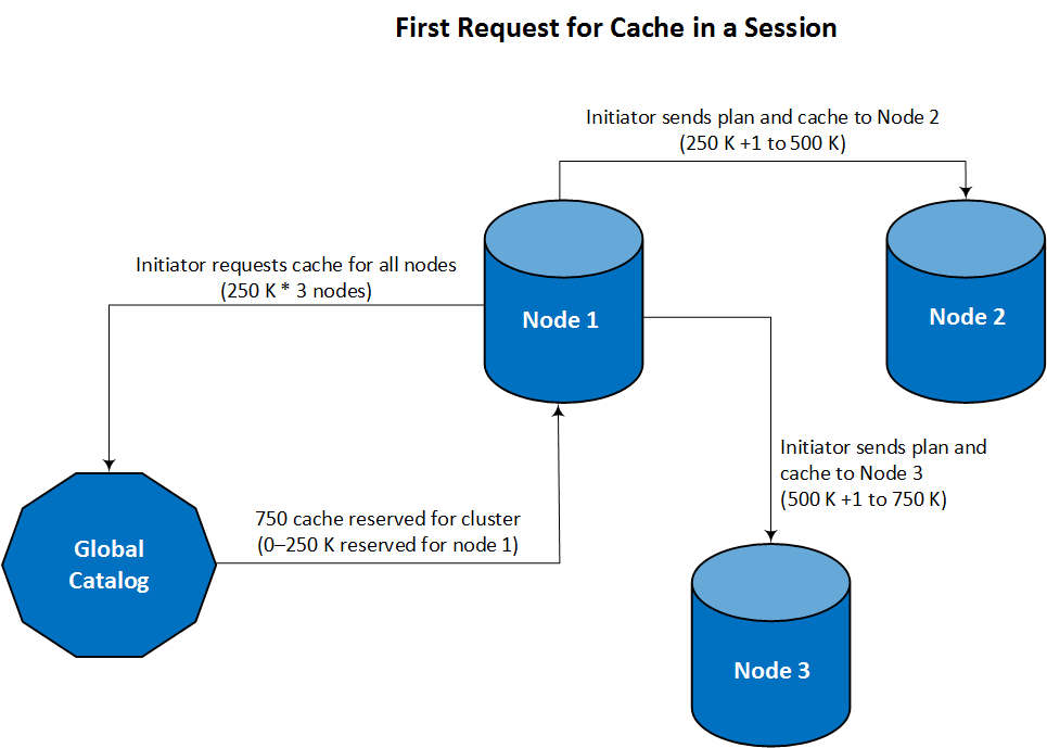
Nodes run out of cache at different times. While executing the same query, nodes individually request additional cache as needed.
For new queries in the same session, the initiator might have an empty cache if it used all of its cache to execute the previous query execution. In this case, the initiator requests cache for all nodes.
Configuring sequence caching
You can change how nodes obtain sequence caches by setting the configuration parameter ClusterSequenceCacheMode to 0 (disabled). When this parameter is set to 0, all nodes in the cluster request their own cache and catalog lock. However, for initial large INSERT-SELECT and COPY operations, when the cache is empty for all nodes, each node requests cache at the same time. These multiple requests result in simultaneous locks on the global catalog, which can adversely affect performance. For this reason, ClusterSequenceCacheMode should remain set to its default value of 1 (enabled).
The following example compares how different settings of ClusterSequenceCacheMode affect how Vertica manages sequence caching. The example assumes a three-node cluster, 250 K caches for each node (the default), and sequence ID values that increment by 1.
|
Workflow step |
ClusterSequenceCacheMode = 1 |
ClusterSequenceCacheMode = 0 |
|
1 |
Cache is empty for all nodes.
Initiator node requests 250 K cache for each node.
|
Cache is empty for all nodes.
Each node, including initiator, requests its own 250 K cache.
|
|
2 |
Blocks of cache are distributed to each node as follows:
Each node begins to use its cache as it processes sequence updates.
|
|
3 |
Initiator node and node 3 run out of cache.
Node 2 only uses 250 K +1 to 400 K, 100 K of cache remains from 400 K +1 to 500 K.
|
|
4 |
Executing same statement:
-
As each node uses up its cache, it requests a new cache allocation.
-
If node 2 never uses its cache, the 100-K unused cache becomes a gap in sequence IDs.
Executing a new statement in same session, if initiator node cache is empty:
-
It requests and distributes new cache blocks for all nodes.
-
Nodes receive a new cache before the old cache is used, creating a gap in ID sequencing.
|
Executing same or new statement:
-
As each node uses up its cache, it requests a new cache allocation.
-
If node 2 never uses its cache, the 100 K unused cache becomes a gap in sequence IDs.
|
7.9 - Merging table data
MERGE statements can perform update and insert operations on a target table based on the results of a join with a source data set.
MERGE statements can perform update and insert operations on a target table based on the results of a join with a source data set. The join can match a source row with only one target row; otherwise, Vertica returns an error.
MERGE has the following syntax:
MERGE INTO target‑table USING source‑dataset ON join-condition
matching‑clause[ matching‑clause ]
Merge operations have at least three components:
7.9.1 - Basic MERGE example
In this example, a merge operation involves two tables:.
In this example, a merge operation involves two tables:
-
visits_daily logs daily restaurant traffic, and is updated with each customer visit. Data in this table is refreshed every 24 hours.
-
visits_history stores the history of customer visits to various restaurants, accumulated over an indefinite time span.
Each night, you merge the daily visit count from visits_daily into visits_history. The merge operation modifies the target table in two ways:
One MERGE statement executes both operations as a single (upsert) transaction.
Source and target tables
The source and target tables visits_daily and visits_history are defined as follows:
CREATE TABLE public.visits_daily
(
customer_id int,
location_name varchar(20),
visit_time time(0) DEFAULT (now())::timetz(6)
);
CREATE TABLE public.visits_history
(
customer_id int,
location_name varchar(20),
visit_count int
);
Table visits_history contains rows of three customers who between them visited two restaurants, Etoile and LaRosa:
=> SELECT * FROM visits_history ORDER BY customer_id, location_name;
customer_id | location_name | visit_count
-------------+---------------+-------------
1001 | Etoile | 2
1002 | La Rosa | 4
1004 | Etoile | 1
(3 rows)
By close of business, table visits_daily contains three rows of restaurant visits:
=> SELECT * FROM visits_daily ORDER BY customer_id, location_name;
customer_id | location_name | visit_time
-------------+---------------+------------
1001 | Etoile | 18:19:29
1003 | Lux Cafe | 08:07:00
1004 | La Rosa | 11:49:20
(3 rows)
Table data merge
The following MERGE statement merges visits_daily data into visits_history:
-
For matching customers, MERGE updates the occurrence count.
-
For non-matching customers, MERGE inserts new rows.
=> MERGE INTO visits_history h USING visits_daily d
ON (h.customer_id=d.customer_id AND h.location_name=d.location_name)
WHEN MATCHED THEN UPDATE SET visit_count = h.visit_count + 1
WHEN NOT MATCHED THEN INSERT (customer_id, location_name, visit_count)
VALUES (d.customer_id, d.location_name, 1);
OUTPUT
--------
3
(1 row)
MERGE returns the number of rows updated and inserted. In this case, the returned value specifies three updates and inserts:
-
Customer 1001's third visit to Etoile
-
New customer 1003's first visit to new restaurant Lux Cafe
-
Customer 1004's first visit to La Rosa
If you now query table visits_history, the result set shows the merged (updated and inserted) data. Updated and new rows are highlighted:
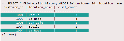
7.9.2 - MERGE source options
A MERGE operation joins the target table to one of the following data sources:.
A MERGE operation joins the target table to one of the following data sources:
-
Another table
-
View
-
Subquery result set
Merging from table and view data
You merge data from one table into another as follows:
MERGE INTO target‑table USING { source‑table | source‑view } join-condition
matching‑clause[ matching‑clause ]
If you specify a view, Vertica expands the view name to the query that it encapsulates, and uses the result set as the merge source data.
For example, the VMart table public.product_dimension contains current and discontinued products. You can move all discontinued products into a separate table public.product_dimension_discontinued, as follows:
=> CREATE TABLE public.product_dimension_discontinued (
product_key int,
product_version int,
sku_number char(32),
category_description char(32),
product_description varchar(128));
=> MERGE INTO product_dimension_discontinued tgt
USING product_dimension src ON tgt.product_key = src.product_key
AND tgt.product_version = src.product_version
WHEN NOT MATCHED AND src.discontinued_flag='1' THEN INSERT VALUES
(src.product_key,
src.product_version,
src.sku_number,
src.category_description,
src.product_description);
OUTPUT
--------
1186
(1 row)
Source table product_dimension uses two columns, product_key and product_version, to identify unique products. The MERGE statement joins the source and target tables on these columns in order to return single instances of non-matching rows. The WHEN NOT MATCHED clause includes a filter (src.discontinued_flag='1'), which reduces the result set to include only discontinued products. The remaining rows are inserted into target table product_dimension_discontinued.
Merging from a subquery result set
You can merge into a table the result set that is returned by a subquery, as follows:
MERGE INTO target‑table USING (subquery) sq-alias join-condition
matching‑clause[ matching‑clause ]
For example, the VMart table public.product_dimension is defined as follows (DDL truncated):
CREATE TABLE public.product_dimension
(
product_key int NOT NULL,
product_version int NOT NULL,
product_description varchar(128),
sku_number char(32),
...
)
ALTER TABLE public.product_dimension
ADD CONSTRAINT C_PRIMARY PRIMARY KEY (product_key, product_version) DISABLED;
Columns product_key and product_version comprise the table's primary key. You can modify this table so it contains a single column that concatenates the values of these two columns. This column can be used to uniquely identify each product, while also maintaining the original values from product_key and product_version.
You populate the new column with a MERGE statement that queries the other two columns:
=> ALTER TABLE public.product_dimension ADD COLUMN product_ID numeric(8,2);
ALTER TABLE
=> MERGE INTO product_dimension tgt
USING (SELECT (product_key||'.0'||product_version)::numeric(8,2) AS pid, sku_number
FROM product_dimension) src
ON tgt.product_key||'.0'||product_version::numeric=src.pid
WHEN MATCHED THEN UPDATE SET product_ID = src.pid;
OUTPUT
--------
60000
(1 row)
The following query verifies that the new column values correspond to the values in product_key and product_version:
=> SELECT product_ID, product_key, product_version, product_description
FROM product_dimension
WHERE category_description = 'Medical'
AND product_description ILIKE '%diabetes%'
AND discontinued_flag = 1 ORDER BY product_ID;
product_ID | product_key | product_version | product_description
------------+-------------+-----------------+-----------------------------------------
5836.02 | 5836 | 2 | Brand #17487 diabetes blood testing kit
14320.02 | 14320 | 2 | Brand #43046 diabetes blood testing kit
18881.01 | 18881 | 1 | Brand #56743 diabetes blood testing kit
(3 rows)
7.9.3 - MERGE matching clauses
MERGE supports one instance of the following matching clauses:.
MERGE supports one instance of the following matching clauses:
Each matching clause can specify an additional filter, as described in Update and insert filters.
WHEN MATCHED THEN UPDATE SET
Updates all target table rows that are joined to the source table, typically with data from the source table:
WHEN MATCHED [ AND update-filter ] THEN UPDATE
SET { target‑column = expression }[,...]
Vertica can execute the join only on unique values in the source table's join column. If the source table's join column contains more than one matching value, the MERGE statement returns with a run-time error.
WHEN NOT MATCHED THEN INSERT
WHEN NOT MATCHED THEN INSERT inserts into the target table a new row for each source table row that is excluded from the join:
WHEN NOT MATCHED [ AND insert-filter ] THEN INSERT
[ ( column‑list ) ] VALUES ( values‑list )
column‑list is a comma-delimited list of one or more target columns in the target table, listed in any order. MERGE maps column‑list columns to values‑list values in the same order, and each column-value pair must be compatible. If you omit column‑list, Vertica maps values‑list values to columns according to column order in the table definition.
For example, given the following source and target table definitions:
CREATE TABLE t1 (a int, b int, c int);
CREATE TABLE t2 (x int, y int, z int);
The following WHEN NOT MATCHED clause implicitly sets the values of the target table columns a, b, and c in the newly inserted rows:
MERGE INTO t1 USING t2 ON t1.a=t2.x
WHEN NOT MATCHED THEN INSERT VALUES (t2.x, t2.y, t2.z);
In contrast, the following WHEN NOT MATCHED clause excludes columns t1.b and t2.y from the merge operation. The WHEN NOT MATCHED clause explicitly pairs two sets of columns from the target and source tables: t1.a to t2.x, and t1.c to t2.z. Vertica sets excluded column t1.b. to null:
MERGE INTO t1 USING t2 ON t1.a=t2.x
WHEN NOT MATCHED THEN INSERT (a, c) VALUES (t2.x, t2.z);
7.9.4 - Update and insert filters
Each WHEN MATCHED and WHEN NOT MATCHED clause in a MERGE statement can optionally specify an update filter and insert filter, respectively:.
Each WHEN MATCHED and WHEN NOT MATCHED clause in a MERGE statement can optionally specify an update filter and insert filter, respectively:
WHEN MATCHED AND update-filter THEN UPDATE ...
WHEN NOT MATCHED AND insert-filter THEN INSERT ...
Vertica also supports Oracle syntax for specifying update and insert filters:
WHEN MATCHED THEN UPDATE SET column-updates WHERE update-filter
WHEN NOT MATCHED THEN INSERT column-values WHERE insert-filter
Each filter can specify multiple conditions. Vertica handles the filters as follows:
-
An update filter is applied to the set of matching rows in the target table that are returned by the MERGE join. For each row where the update filter evaluates to true, Vertica updates the specified columns.
-
An insert filter is applied to the set of source table rows that are excluded from the MERGE join. For each row where the insert filter evaluates to true, Vertica adds a new row to the target table with the specified values.
For example, given the following data in tables t11 and t22:
=> SELECT * from t11 ORDER BY pk;
pk | col1 | col2 | SKIP_ME_FLAG
----+------+------+--------------
1 | 2 | 3 | t
2 | 3 | 4 | t
3 | 4 | 5 | f
4 | | 6 | f
5 | 6 | 7 | t
6 | | 8 | f
7 | 8 | | t
(7 rows)
=> SELECT * FROM t22 ORDER BY pk;
pk | col1 | col2
----+------+------
1 | 2 | 4
2 | 4 | 8
3 | 6 |
4 | 8 | 16
(4 rows)
You can merge data from table t11 into table t22 with the following MERGE statement, which includes update and insert filters:
=> MERGE INTO t22 USING t11 ON ( t11.pk=t22.pk )
WHEN MATCHED
AND t11.SKIP_ME_FLAG=FALSE AND (
COALESCE (t22.col1<>t11.col1, (t22.col1 is null)<>(t11.col1 is null))
)
THEN UPDATE SET col1=t11.col1, col2=t11.col2
WHEN NOT MATCHED
AND t11.SKIP_ME_FLAG=FALSE
THEN INSERT (pk, col1, col2) VALUES (t11.pk, t11.col1, t11.col2);
OUTPUT
--------
3
(1 row)
=> SELECT * FROM t22 ORDER BY pk;
pk | col1 | col2
----+------+------
1 | 2 | 4
2 | 4 | 8
3 | 4 | 5
4 | | 6
6 | | 8
(5 rows)
Vertica uses the update and insert filters as follows:
-
Evaluates all matching rows against the update filter conditions. Vertica updates each row where the following two conditions both evaluate to true:
-
Evaluates all non-matching rows in the source table against the insert filter. For each row where column t11.SKIP_ME_FLAG is set to false, Vertica inserts a new row in the target table.
7.9.5 - MERGE optimization
You can improve MERGE performance in several ways:.
You can improve MERGE performance in several ways:
Projections for MERGE operations
The Vertica query optimizer automatically chooses the best projections to implement a merge operation. A good projection design strategy provides projections that help the query optimizer avoid extra sort and data transfer operations, and facilitate MERGE performance.
For example, the following MERGE statement fragment joins source and target tables tgt and src, respectively, on columns tgt.a and src.b:
=> MERGE INTO tgt USING src ON tgt.a = src.b ...
Vertica can use a local merge join if projections for tables tgt and src use one of the following projection designs, where inputs are presorted by projection ORDER BY clauses:
Optimizing MERGE query plans
Vertica prepares an optimized query plan if the following conditions are all true:
-
The MERGE statement contains both matching clauses
WHEN MATCHED THEN UPDATE SET and
WHEN NOT MATCHED THEN INSERT. If the MERGE statement contains only one matching clause, it uses a non-optimized query plan.
-
The MERGE statement excludes update and insert filters.
-
The target table join column has a unique or primary key constraint. This requirement does not apply to the source table join column.
-
Both matching clauses specify all columns in the target table.
-
Both matching clauses specify identical source values.
For details on evaluating an
EXPLAIN-generated query plan, see MERGE path.
The examples that follow use a simple schema to illustrate some of the conditions under which Vertica prepares or does not prepare an optimized query plan for MERGE:
CREATE TABLE target(a INT PRIMARY KEY, b INT, c INT) ORDER BY b,a;
CREATE TABLE source(a INT, b INT, c INT) ORDER BY b,a;
INSERT INTO target VALUES(1,2,3);
INSERT INTO target VALUES(2,4,7);
INSERT INTO source VALUES(3,4,5);
INSERT INTO source VALUES(4,6,9);
COMMIT;
Optimized MERGE statement
Vertica can prepare an optimized query plan for the following MERGE statement because:
-
The target table's join column t.a has a primary key constraint.
-
All columns in the target table (a,b,c) are included in the UPDATE and INSERT clauses.
-
The UPDATE and INSERT clauses specify identical source values: s.a, s.b, and s.c.
MERGE INTO target t USING source s ON t.a = s.a
WHEN MATCHED THEN UPDATE SET a=s.a, b=s.b, c=s.c
WHEN NOT MATCHED THEN INSERT(a,b,c) VALUES(s.a, s.b, s.c);
OUTPUT
--------
2
(1 row)
The output value of 2 indicates success and denotes the number of rows updated/inserted from the source into the target.
Non-optimized MERGE statement
In the next example, the MERGE statement runs without optimization because the source values in the UPDATE/INSERT clauses are not identical. Specifically, the UPDATE clause includes constants for columns s.a and s.c and the INSERT clause does not:
MERGE INTO target t USING source s ON t.a = s.a
WHEN MATCHED THEN UPDATE SET a=s.a + 1, b=s.b, c=s.c - 1
WHEN NOT MATCHED THEN INSERT(a,b,c) VALUES(s.a, s.b, s.c);
To make the previous MERGE statement eligible for optimization, rewrite the statement so that the source values in the UPDATE and INSERT clauses are identical:
MERGE INTO target t USING source s ON t.a = s.a
WHEN MATCHED THEN UPDATE SET a=s.a + 1, b=s.b, c=s.c -1
WHEN NOT MATCHED THEN INSERT(a,b,c) VALUES(s.a + 1, s.b, s.c - 1);
7.9.6 - MERGE restrictions
The following restrictions apply to updating and inserting table data with MERGE.
The following restrictions apply to updating and inserting table data with
MERGE.
Constraint enforcement
If primary key, unique key, or check constraints are enabled for automatic enforcement in the target table, Vertica enforces those constraints when you load new data. If a violation occurs, Vertica rolls back the operation and returns an error.
Caution
If you run MERGE multiple times using the same target and source table, each iteration is liable to introduce duplicate values into the target columns and return with an error.
Columns prohibited from merge
The following columns cannot be specified in a merge operation; attempts to do so return with an error:
-
IDENTITY columns, or columns whose default value is set to a named sequence.
-
Vmap columns such as __raw__ in flex tables.
-
Columns of complex types ARRAY, SET, or ROW.
7.10 - Removing table data
Vertica provides several ways to remove data from a table:.
Vertica provides several ways to remove data from a table:
|
Delete operation |
Description |
|
Drop a table |
Permanently remove a table and its definition, optionally remove associated views and projections. |
|
Delete table rows |
Mark rows with delete vectors and store them so data can be rolled back to a previous epoch. The data must be purged to reclaim disk space. |
|
Truncate table data |
Remove all storage and history associated with a table. The table structure is preserved for future use. |
|
Purge data |
Permanently remove historical data from physical storage and free disk space for reuse. |
|
Drop partitions |
Remove one more partitions from a table. Each partition contains a related subset of data in the table. Dropping partitioned data is efficient, and provides query performance benefits. |
7.10.1 - Data removal operations compared
/need to include purge operations? or is that folded into DELETE operations?/.
The following table summarizes differences between various data removal operations.
|
Operations and options |
Performance |
Auto commits |
Saves history |
DELETE FROM ``table |
Normal |
No |
Yes |
DELETE FROM ``temp‑table |
High |
No |
No |
DELETE FROM table where-clause |
Normal |
No |
Yes |
DELETE FROM temp‑table where-clause |
Normal |
No |
Yes |
DELETE FROM temp‑table where-clause
ON COMMIT PRESERVE ROWS
|
Normal |
No |
Yes |
DELETE FROM temp‑table where-clause
ON COMMIT DELETE ROWS
|
High |
Yes |
No |
DROP table |
High |
Yes |
No |
TRUNCATE table |
High |
Yes |
No |
TRUNCATE temp‑table |
High |
Yes |
No |
SELECT DROP_PARTITIONS (...) |
High |
Yes |
No |
Choosing the best operation
The following table can help you decide which operation is best for removing table data:
|
If you want to... |
Use... |
|
Delete both table data and definitions and start from scratch. |
DROP TABLE |
|
Quickly drop data while preserving table definitions, and reload data. |
TRUNCATE TABLE |
|
Regularly perform bulk delete operations on logical sets of data. |
DROP_PARTITIONS |
|
Occasionally perform small deletes with the option to roll back or review history. |
DELETE |
7.10.2 - Optimizing DELETE and UPDATE
Vertica is optimized for query-intensive workloads, so DELETE and UPDATE queries might not achieve the same level of performance as other queries.
Vertica is optimized for query-intensive workloads, so DELETE and UPDATE queries might not achieve the same level of performance as other queries. A DELETE and UPDATE operation must update all projections, so the operation can only be as fast as the slowest projection.
To improve the performance of DELETE and UPDATE queries, consider the following issues:
- Query performance after large DELETE operations: Vertica's implementation of DELETE differs from traditional databases: it does not delete data from disk storage; rather, it marks rows as deleted so they are available for historical queries. Deletion of 10% or more of the total rows in a table can adversely affect queries on that table. In that case, consider purging those rows to improve performance.
- Recovery performance: Recovery is the action required for a cluster to restore K-safety after a crash. Large numbers of deleted records can degrade the performance of a recovery. To improve recovery performance, purge the deleted rows.
- Concurrency: DELETE and UPDATE take exclusive locks on the table. Only one DELETE or UPDATE transaction on a table can be in progress at a time and only when no load operations are in progress. Delete and update operations on different tables can run concurrently.
Projection column requirements for optimized delete
A projection is optimized for delete and update operations if it contains all columns required by the query predicate. In general, DML operations are significantly faster when performed on optimized projections than on non-optimized projections.
For example, consider the following table and projections:
=> CREATE TABLE t (a INTEGER, b INTEGER, c INTEGER);
=> CREATE PROJECTION p1 (a, b, c) AS SELECT * FROM t ORDER BY a;
=> CREATE PROJECTION p2 (a, c) AS SELECT a, c FROM t ORDER BY c, a;
In the following query, both p1 and p2 are eligible for DELETE and UPDATE optimization because column a is available:
=> DELETE from t WHERE a = 1;
In the following example, only projection p1 is eligible for DELETE and UPDATE optimization because the b column is not available in p2:
=> DELETE from t WHERE b = 1;
Optimized DELETE in subqueries
To be eligible for DELETE optimization, all target table columns referenced in a DELETE or UPDATE statement's WHERE clause must be in the projection definition.
For example, the following simple schema has two tables and three projections:
=> CREATE TABLE tb1 (a INT, b INT, c INT, d INT);
=> CREATE TABLE tb2 (g INT, h INT, i INT, j INT);
The first projection references all columns in tb1 and sorts on column a:
=> CREATE PROJECTION tb1_p AS SELECT a, b, c, d FROM tb1 ORDER BY a;
The buddy projection references and sorts on column a in tb1:
=> CREATE PROJECTION tb1_p_2 AS SELECT a FROM tb1 ORDER BY a;
This projection references all columns in tb2 and sorts on column i:
=> CREATE PROJECTION tb2_p AS SELECT g, h, i, j FROM tb2 ORDER BY i;
Consider the following DML statement, which references tb1.a in its WHERE clause. Since both projections on tb1 contain column a, both are eligible for the optimized DELETE:
=> DELETE FROM tb1 WHERE tb1.a IN (SELECT tb2.i FROM tb2);
Restrictions
Optimized DELETE operations are not supported under the following conditions:
-
With replicated projections if subqueries reference the target table. For example, the following syntax is not supported:
=> DELETE FROM tb1 WHERE tb1.a IN (SELECT e FROM tb2, tb2 WHERE tb2.e = tb1.e);
-
With subqueries that do not return multiple rows. For example, the following syntax is not supported:
=> DELETE FROM tb1 WHERE tb1.a = (SELECT k from tb2);
Projection sort order for optimizing DELETE
Design your projections so that frequently-used DELETE or UPDATE predicate columns appear in the sort order of all projections for large DELETE and UPDATE operations.
For example, suppose most of the DELETE queries you perform on a projection look like the following:
=> DELETE from t where time_key < '1-1-2007'
To optimize the delete operations, make time_key appear in the ORDER BY clause of all projections. This schema design results in better performance of the delete operation.
In addition, add sort columns to the sort order such that each combination of the sort key values uniquely identifies a row or a small set of rows. For more information, see Choosing sort order: best practices. To analyze projections for sort order issues, use the EVALUATE_DELETE_PERFORMANCE function.
7.10.3 - Purging deleted data
In Vertica, delete operations do not remove rows from physical storage.
In Vertica, delete operations do not remove rows from physical storage. DELETE marks rows as deleted, as does UPDATE, which combines delete and insert operations. In both cases, Vertica retains discarded rows as historical data, which remains accessible to historical queries until it is purged.
The cost of retaining historical data is twofold:
-
Disk space is allocated to deleted rows and delete markers.
-
Typical (non-historical) queries must read and skip over deleted data, which can impact performance.
A purge operation permanently removes historical data from physical storage and frees disk space for reuse. Only historical data that precedes the Ancient History Mark (AHM) is eligible to be purged.
You can purge data in two ways:
In both cases, Vertica purges all historical data up to and including the AHM epoch and resets the AHM. See Epochs for additional information about how Vertica uses epochs.
Caution
Large delete and purge operations can take a long time to complete, so use them sparingly. If your application requires deleting data on a regular basis, such as by month or year, consider designing tables that take advantage of
table partitioning. If partitioning is not suitable, consider
rebuilding the table.
7.10.3.1 - Setting a purge policy
The preferred method for purging data is to establish a policy that determines which deleted data is eligible to be purged.
The preferred method for purging data is to establish a policy that determines which deleted data is eligible to be purged. Eligible data is automatically purged when the Tuple Mover performs mergeout operations.
Vertica provides two methods for determining when deleted data is eligible to be purged:
Specifying the time for which delete data is saved
Specifying the time for which delete data is saved is the preferred method for determining which deleted data can be purged. By default, Vertica saves historical data only when nodes are down.
To change the specified time for saving deleted data, use the HistoryRetentionTime configuration parameter:
=> ALTER DATABASE DEFAULT SET HistoryRetentionTime = {seconds | -1};
In the above syntax:
-
seconds is the amount of time (in seconds) for which to save deleted data.
-
-1 indicates that you do not want to use the HistoryRetentionTime configuration parameter to determine which deleted data is eligible to be purged. Use this setting if you prefer to use the other method (HistoryRetentionEpochs) for determining which deleted data can be purged.
The following example sets the history epoch retention level to 240 seconds:
=> ALTER DATABASE DEFAULT SET HistoryRetentionTime = 240;
Specifying the number of epochs that are saved
Unless you have a reason to limit the number of epochs, Vertica recommends that you specify the time over which delete data is saved.
To specify the number of historical epoch to save through the HistoryRetentionEpochs configuration parameter:
-
Turn off the HistoryRetentionTime configuration parameter:
=> ALTER DATABASE DEFAULT SET HistoryRetentionTime = -1;
-
Set the history epoch retention level through the HistoryRetentionEpochs configuration parameter:
=> ALTER DATABASE DEFAULT SET HistoryRetentionEpochs = {num_epochs | -1};
-
num_epochs is the number of historical epochs to save.
-
-1 indicates that you do not want to use the HistoryRetentionEpochs configuration parameter to trim historical epochs from the epoch map. By default, HistoryRetentionEpochs is set to -1.
The following example sets the number of historical epochs to save to 40:
=> ALTER DATABASE DEFAULT SET HistoryRetentionEpochs = 40;
Modifications are immediately implemented across all nodes within the database cluster. You do not need to restart the database.
Note
If both HistoryRetentionTime and HistoryRetentionEpochs are specified, HistoryRetentionTime takes precedence.
See Epoch management parameters for additional details. See Epochs for information about how Vertica uses epochs.
Disabling purge
If you want to preserve all historical data, set the value of both historical epoch retention parameters to -1, as follows:
=> ALTER DABABASE mydb SET HistoryRetentionTime = -1;
=> ALTER DATABASE DEFAULT SET HistoryRetentionEpochs = -1;
7.10.3.2 - Manually purging data
You manually purge deleted data as follows:.
You manually purge deleted data as follows:
-
Set the cut-off date for purging deleted data. First, call one of the following functions to verify the current ancient history mark (AHM):
-
Set the AHM to the desired cut-off date with one of the following functions:
If you call SET_AHM_TIME, keep in mind that the timestamp you specify is mapped to an epoch, which by default has a three-minute granularity. Thus, if you specify an AHM time of 2008-01-01 00:00:00.00, Vertica might purge data from the first three minutes of 2008, or retain data from last three minutes of 2007.
Note
You cannot advance the AHM beyond a point where Vertica is unable to recover data for a down node.
-
Purge deleted data from the desired projections with one of the following functions:
The tuple mover performs a mergeout operation to purge the data. Vertica periodically invokes the tuple mover to perform mergeout operations, as configured by tuple mover parameters. You can manually invoke the tuple mover by calling the function
DO_TM_TASK.
Caution
Manual purge operations can take a long time.
See Epochs for additional information about how Vertica uses epochs.
7.10.4 - Truncating tables
TRUNCATE TABLE removes all storage associated with the target table and its projections.
TRUNCATE TABLE removes all storage associated with the target table and its projections. Vertica preserves the table and the projection definitions. If the truncated table has out-of-date projections, those projections are cleared and marked up-to-date when TRUNCATE TABLE returns.
TRUNCATE TABLE commits the entire transaction after statement execution, even if truncating the table fails. You cannot roll back a TRUNCATE TABLE statement.
Use TRUNCATE TABLE for testing purposes. You can use it to remove all data from a table and load it with fresh data, without recreating the table and its projections.
Table locking
TRUNCATE TABLE takes an O (owner) lock on the table until the truncation process completes. The savepoint is then released.
If the operation cannot obtain an O lock on the target table, Vertica tries to close any internal Tuple Mover sessions that are running on that table. If successful, the operation can proceed. Explicit Tuple Mover operations that are running in user sessions do not close. If an explicit Tuple Mover operation is running on the table, the operation proceeds only when the operation is complete.
Restrictions
You cannot truncate an external table.
Examples
=> INSERT INTO sample_table (a) VALUES (3);
=> SELECT * FROM sample_table;
a
---
3
(1 row)
=> TRUNCATE TABLE sample_table;
TRUNCATE TABLE
=> SELECT * FROM sample_table;
a
---
(0 rows)
7.11 - Rebuilding tables
You can reclaim disk space on a large scale by rebuilding tables, as follows:.
You can reclaim disk space on a large scale by rebuilding tables, as follows:
-
Create a table with the same (or similar) definition as the table to rebuild.
-
Create projections for the new table.
-
Copy data from the target table into the new one with
INSERT...SELECT.
-
Drop the old table and its projections.
Note
Rather than dropping the old table, you can rename it and use it as a backup copy. Before doing so, verify that you have sufficient disk space for both the new and old tables.
-
Rename the new table with
ALTER TABLE...RENAME, using the name of the old table.
Caution
When you rebuild a table, Vertica purges the table of all delete vectors that precede the AHM. This prevents historical queries on any older epoch.
Projection considerations
-
You must have enough disk space to contain the old and new projections at the same time. If necessary, you can drop some of the old projections before loading the new table. You must, however, retain at least one superprojection of the old table (or two buddy superprojections to maintain K-safety) until the new table is loaded. (See
Prepare Disk Storage Locations for disk space requirements.)
-
You can specify different names for the new projections or use ALTER TABLE...RENAME to change the names of the old projections.
-
The relationship between tables and projections does not depend on object names. Instead, it depends on object identifiers that are not affected by rename operations. Thus, if you rename a table, its projections continue to work normally.
7.12 - Dropping tables
DROP TABLE drops a table from the database catalog.
DROP TABLE drops a table from the database catalog. If any projections are associated with the table, DROP TABLE returns an error message unless it also includes the CASCADE option. One exception applies: the table only has an auto-generated superprojection (auto-projection) associated with it.
Using CASCADE
In the following example, DROP TABLE tries to remove a table that has several projections associated with it. Because it omits the CASCADE option, Vertica returns an error:
=> DROP TABLE d1;
NOTICE: Constraint - depends on Table d1
NOTICE: Projection d1p1 depends on Table d1
NOTICE: Projection d1p2 depends on Table d1
NOTICE: Projection d1p3 depends on Table d1
NOTICE: Projection f1d1p1 depends on Table d1
NOTICE: Projection f1d1p2 depends on Table d1
NOTICE: Projection f1d1p3 depends on Table d1
ERROR: DROP failed due to dependencies: Cannot drop Table d1 because other objects depend on it
HINT: Use DROP ... CASCADE to drop the dependent objects too.
=> DROP TABLE d1 CASCADE;
DROP TABLE
=> CREATE TABLE mytable (a INT, b VARCHAR(256));
CREATE TABLE
=> DROP TABLE IF EXISTS mytable;
DROP TABLE
=> DROP TABLE IF EXISTS mytable; -- Doesn't exist
NOTICE: Nothing was dropped
DROP TABLE
The next attempt includes the CASCADE option and succeeds:
=> DROP TABLE d1 CASCADE;
DROP TABLE
=> CREATE TABLE mytable (a INT, b VARCHAR(256));
CREATE TABLE
=> DROP TABLE IF EXISTS mytable;
DROP TABLE
=> DROP TABLE IF EXISTS mytable; -- Doesn't exist
NOTICE: Nothing was dropped
DROP TABLE
Using IF EXISTS
In the following example, DROP TABLE includes the option IF EXISTS. This option specifies not to report an error if one or more of the tables to drop does not exist. This clause is useful in SQL scripts—for example, to ensure that a table is dropped before you try to recreate it:
=> DROP TABLE IF EXISTS mytable;
DROP TABLE
=> DROP TABLE IF EXISTS mytable; -- Table doesn't exist
NOTICE: Nothing was dropped
DROP TABLE
Dropping and restoring view tables
Views that reference a table that is dropped and then replaced by another table with the same name continue to function and use the contents of the new table. The new table must have the same column definitions.
8 - Managing client connections
Vertica provides several settings to control client connections:.
Vertica provides several settings to control client connections:
-
Limit the number of client connections a user can have open at the same time.
-
Limit the time a client connection can be idle before being automatically disconnected.
-
Use connection load balancing to spread the overhead of servicing client connections among nodes.
-
Detect unresponsive clients with TCP keepalive.
-
Drain a subcluster to reject any new client connections to that subcluster. For details, see Drain client connections.
Total client connections to a given node cannot exceed the limits set in MaxClientSessions.
Changes to a client's MAXCONNECTIONS property have no effect on current sessions; these changes apply only to new sessions. For example, if you change user's connection mode from DATABASE to NODE, current node connections are unaffected. This change applies only to new sessions, which are reserved on the invoking node.
When Vertica closes a client connection, the client's ongoing operations, if any, are canceled.
8.1 - Limiting the number and length of client connections
You can manage how many active sessions a user can open to the server, and the duration of those sessions.
You can manage how many active sessions a user can open to the server, and the duration of those sessions. Doing so helps prevent overuse of available resources, and can improve overall throughput.
You can define connection limits at two levels:
-
Set the MAXCONNECTIONS property on individual users. This property specifies how many sessions a user can open concurrently on individual nodes, or across the database cluster. For example, the following ALTER USER statement allows user Joe up to 10 concurrent sessions:
=> ALTER USER Joe MAXCONNECTIONS 10 ON DATABASE;
-
Set the configuration parameter MaxClientSessions on the database or individual nodes. This parameter specifies the maximum number of client sessions that can run on nodes in the database cluster, by default set to 50. An extra five sessions are always reserved to dbadmin users. This enables them to log in when the total number of client sessions equals MaxClientSessions.
Total client connections to a given node cannot exceed the limits set in MaxClientSessions.
Changes to a client's MAXCONNECTIONS property have no effect on current sessions; these changes apply only to new sessions. For example, if you change user's connection mode from DATABASE to NODE, current node connections are unaffected. This change applies only to new sessions, which are reserved on the invoking node.
Managing TCP keepalive settings
Vertica uses kernel TCP keepalive parameters to detect unresponsive clients and determine when the connection should be closed.Vertica also supports a set of equivalent KeepAlive parameters that can override TCP keepalive parameter settings. By default, all Vertica KeepAlive parameters are set to 0, which signifies to use TCP keepalive settings. To override TCP keepalive settings, set the equivalent parameters at the database level with ALTER DATABASE, or for the current session with ALTER SESSION.
|
TCP keepalive Parameter |
Vertica Parameter |
Description |
|
tcp_keepalive_time |
KeepAliveIdleTime |
Length (in seconds) of the idle period before the first TCP keepalive probe is sent to ensure that the client is still connected. |
|
tcp_keepalive_probes |
KeepAliveProbeCount |
Number of consecutive keepalive probes that must go unacknowledged by the client before the client connection is considered lost and closed |
|
tcp_keepalive_intvl |
KeepAliveProbeInterval |
Time interval (in seconds) between keepalive probes. |
Examples
The following examples show how to use Vertica KeepAlive parameters to override TCP keepalive parameters as follows:
-
After 600 seconds (ten minutes), the first keepalive probe is sent to the client.
-
Consecutive keepalive probes are sent every 30 seconds.
-
If the client fails to respond to 10 keepalive probes, the connection is considered lost and is closed.
To make this the default policy for client connections, use ALTER DATABASE:
=> ALTER DATABASE DEFAULT SET KeepAliveIdleTime = 600;
=> ALTER DATABASE DEFAULT SET KeepAliveProbeInterval = 30;
=> ALTER DATABASE DEFAULT SET KeepAliveProbeCount = 10;
To override database-level policies for the current session, use ALTER SESSION:
=> ALTER SESSION SET KeepAliveIdleTime = 400;
=> ALTER SESSION SET KeepAliveProbeInterval = 72;
=> ALTER SESSION SET KeepAliveProbeCount = 60;
Query system table CONFIGURATION_PARAMETERS to verify database and session settings of the three Vertica KeepAlive parameters:
=> SELECT parameter_name, database_value, current_value FROM configuration_parameters WHERE parameter_name ILIKE 'KeepAlive%';
parameter_name | database_value | current_value
------------------------+----------------+---------------
KeepAliveProbeCount | 10 | 60
KeepAliveIdleTime | 600 | 400
KeepAliveProbeInterval | 30 | 72
(3 rows)
Limiting idle session length
If a client continues to respond to TCP keepalive probes, but is not running any queries, the client's session is considered idle. Idle sessions eventually time out. The maximum time that sessions are allowed to idle can be set at three levels, in descending order of precedence:
- As dbadmin, set the IDLESESSIONTIMEOUT property for individual users. This property overrides all other session timeout settings.
- Users can limit the idle time of the current session with SET SESSION IDLESESSIONTIMEOUT. Non-superusers can only set their session idle time to a value equal to or lower than their own IDLESESSIONTIMEOUT setting. If no session idle time is explicitly set for a user, the session idle time for that user is inherited from the node or database settings.
- As dbadmin, set configuration parameter DEFAULTIDLESESSIONTIMEOUT. on the database or on individual nodes. This You can limit the default database cluster or individual nodes, with configuration parameter DEFAULTIDLESESSIONTIMEOUT. This parameter sets the default timeout value for all non-superusers.
All settings apply to sessions that are continuously idle—that is, sessions where no queries are running. If a client is slow or unresponsive during query execution, that time does not apply to timeouts. For example, the time that is required for a streaming batch insert is not counted towards timeout. The server identifies a session as idle starting from the moment it starts to wait for any type of message from that session.
Viewing session settings
|
Session length limits |
Database
=> SHOW DATABASE DEFAULT DEFAULTIDLESESSIONTIMEOUT;
name | setting
---------------------------+---------
DefaultIdleSessionTimeout | 2 day
(1 row)
Current session
=> SHOW IDLESESSIONTIMEOUT;
name | setting
--------------------+---------
idlesessiontimeout | 1
(1 row)
|
|
Connection limits |
Database
=> SHOW DATABASE DEFAULT MaxClientSessions;
name | setting
-------------------+---------
MaxClientSessions | 50
(1 row)
User
=> SELECT user_name, max_connections, connection_limit_mode FROM users
WHERE user_name != 'dbadmin';
user_name | max_connections | connection_limit_mode
-----------+-----------------+-----------------------
SuzyX | 3 | database
Joe | 10 | database
(2 rows)
|
Closing user sessions
To manually close a user session, use CLOSE_USER_SESSIONS:
=> SELECT CLOSE_USER_SESSIONS ('Joe');
close_user_sessions
------------------------------------------------------------------------------
Close all sessions for user Joe sent. Check v_monitor.sessions for progress.
(1 row)
Example
A user executes a query, and for some reason the query takes an unusually long time to finish (for example, because of server traffic or query complexity). In this case, the user might think the query failed, and opens another session to run the same query. Now, two sessions run the same query, using an extra connection.
To prevent this situation, you can limit how many sessions individual users can run, by modifying their MAXCONNECTIONS user property. This can help minimize the chances of running redundant queries. It also helps prevent users from consuming all available connections, as set by the database For example, the following setting on user SuzyQ limits her to two database sessions at any time:
=> CREATE USER SuzyQ MAXCONNECTIONS 2 ON DATABASE;
Limiting Another issue setting client connections prevents is when a user connects to the server many times. Too many user connections exhausts the number of allowable connections set by database configuration parameter MaxClientSessions.
Note
No user can have a MAXCONNECTIONS limit greater than the MaxClientSessions setting.
Cluster changes and connections
Behavior changes can occur with client connection limits when the following changes occur to a cluster:
Changes in node availability between connection requests have little impact on connection limits.
In terms of honoring connection limits, no significant impact exists when nodes go down or come up in between connection requests. No special actions are needed to handle this. However, if a node goes down, its active session exits and other nodes in the cluster also drop their sessions. This frees up connections. The query may hang in which case the blocked sessions are reasonable and as expected.
8.2 - Drain client connections
Draining client connections in a subclusters prepares the subcluster for shutdown by marking all nodes in the subcluster as draining.
Eon Mode only
Draining client connections in a subclusters prepares the subcluster for shutdown by marking all nodes in the subcluster as draining. Work from existing user sessions continues on draining nodes, but the nodes refuse new client connections and are excluded from load-balancing operations. If clients attempt to connect to a draining node, they receive an error that informs them of the draining status. Load balancing operations exclude draining nodes, so clients that opt-in to connection load balancing should receive a connection error only if all nodes in the load balancing policy are draining. You do not need to change any connection load balancing configurations to use this feature. dbadmin can still connect to draining nodes.
To drain client connections before shutting down a subcluster, you can use the SHUTDOWN_WITH_DRAIN function. This function performs a Graceful Shutdown that marks a subcluster as draining until either the existing connections complete their work and close or a user-specified timeout is reached. When one of these conditions is met, the function proceeds to shutdown the subcluster. Vertica provides several meta-functions that allow you to independently perform each step of the SHUTDOWN_WITH_DRAIN process. You can use the START_DRAIN_SUBCLUSTER function to mark a subcluster as draining and then the SHUTDOWN_SUBCLUSTER function to shut down a subcluster once its connections have closed.
You can use the CANCEL_DRAIN_SUBCLUSTER function to mark all nodes in a subcluster as not draining. As soon as a node is both UP and not draining, the node accepts new client connections. If all nodes in a draining subcluster are down, the draining status of its nodes is automatically reset to not draining.
You can query the DRAINING_STATUS system table to monitor the draining status of each node as well as client connection information, such as the number of active user sessions on each node.
The following example drains a subcluster named analytics, then cancels the draining of the subcluster.
To mark the analytics subcluster as draining, call SHUTDOWN_WITH_DRAIN with a negative timeout value:
=> SELECT SHUTDOWN_WITH_DRAIN('analytics', -1);
NOTICE 0: Draining has started on subcluster (analytics)
You can confirm that the subcluster is draining by querying the DRAINING_STATUS system table:
=> SELECT node_name, subcluster_name, is_draining FROM draining_status ORDER BY 1;
node_name | subcluster_name | is_draining
-------------------+--------------------+--------------
verticadb_node0001 | default_subcluster | f
verticadb_node0002 | default_subcluster | f
verticadb_node0003 | default_subcluster | f
verticadb_node0004 | analytics | t
verticadb_node0005 | analytics | t
verticadb_node0006 | analytics | t
If a client attempts to connect directly to a node in the draining subcluster, they receive the following error message:
$ /opt/vertica/bin/vsql -h noeIP --password password verticadb analyst
vsql: FATAL 10611: New session rejected because subcluster to which this node belongs is draining connections
To cancel the graceful shutdown of the analytics subcluster, you can type Ctrl+C:
=> SELECT SHUTDOWN_WITH_DRAIN('analytics', -1);
NOTICE 0: Draining has started on subcluster (analytics)
^CCancel request sent
ERROR 0: Cancel received after draining started and before shutdown issued. Nodes will not be shut down. The subclusters are still in the draining state.
HINT: Run cancel_drain_subcluster('') to restore all nodes to the 'not_draining' state
As mentioned in the above hint, you can run CANCEL_DRAIN_SUBCLUSTER to reset the status of the draining nodes in the subcluster to not draining:
=> SELECT CANCEL_DRAIN_SUBCLUSTER('analytics');
CANCEL_DRAIN_SUBCLUSTER
--------------------------------------------------------
Targeted subcluster: 'analytics'
Action: CANCEL DRAIN
(1 row)
To confirm that the subcluster is no longer draining, you can again query the
DRAINING_STATUS system table:
=> SELECT node_name, subcluster_name, is_draining FROM draining_status ORDER BY 1;
node_name | subcluster_name | is_draining
-------------------+--------------------+-------
verticadb_node0001 | default_subcluster | f
verticadb_node0002 | default_subcluster | f
verticadb_node0003 | default_subcluster | f
verticadb_node0004 | analytics | f
verticadb_node0005 | analytics | f
verticadb_node0006 | analytics | f
(6 rows)
8.3 - Connection load balancing
Each client connection to a host in the Vertica cluster requires a small overhead in memory and processor time.
Each client connection to a host in the Vertica cluster requires a small overhead in memory and processor time. If many clients connect to a single host, this overhead can begin to affect the performance of the database. You can spread the overhead of client connections by dictating that certain clients connect to specific hosts in the cluster. However, this manual balancing becomes difficult as new clients and hosts are added to your environment.
Connection load balancing helps automatically spread the overhead of client connections across the cluster by having hosts redirect client connections to other hosts. By redirecting connections, the overhead from client connections is spread across the cluster without having to manually assign particular hosts to individual clients. Clients can connect to a small handful of hosts, and they are naturally redirected to other hosts in the cluster. Load balancing does not redirect connections to draining hosts. For more information see, Drain client connections.
Native connection load balancing overview
Native connection load balancing is a feature built into the Vertica Analytic Database server and client libraries as well as vsql. Both the server and the client need to enable load balancing for it to function. If connection load balancing is enabled, a host in the database cluster can redirect a client's attempt to connect to it to another currently-active host in the cluster. This redirection is based on a load balancing policy. This redirection only takes place once, so a client is not bounced from one host to another.
Because native connection load balancing is incorporated into the Vertica client libraries, any client application that connects to Vertica transparently takes advantage of it simply by setting a connection parameter.
How you choose to implement connection load balancing depends on your network environment. Since native load connection balancing is easier to implement, you should use it unless your network configuration requires that clients be separated from the hosts in the Vertica database by a firewall.
For more about native connection load balancing, see About Native Connection Load Balancing.
8.3.1 - About native connection load balancing
Native connection load balancing is a feature built into the Vertica server and client libraries that helps spread the CPU and memory overhead caused by client connections across the hosts in the database.
Native connection load balancing is a feature built into the Vertica server and client libraries that helps spread the CPU and memory overhead caused by client connections across the hosts in the database. It can prevent unequal distribution of client connections among hosts in the cluster.
There are two types of native connection load balancing:
-
Cluster-wide balancing—This method the legacy method of connection load balancing. It was the only type of load balancing prior to Vertica version 9.2. Using this method, you apply a single load balancing policy across the entire cluster. All connection to the cluster are handled the same way.
-
Load balancing policies—This method lets you set different load balancing policies depending on the source of client connection. For example, you can have a policy that redirects connections from outside of your local network to one set of nodes in your cluster, and connections from within your local network to another set of nodes.
8.3.2 - Classic connection load balancing
The classic connection load balancing feature applies a single policy for all client connections to your database.
The classic connection load balancing feature applies a single policy for all client connections to your database. Both your database and the client must enable the load balancing option in order for connections to be load balanced. When both client and server enable load balancing, the following process takes place when the client attempts to open a connection to Vertica:
-
The client connects to a host in the database cluster, with a connection parameter indicating that it is requesting a load-balanced connection.
-
The host chooses a host from the list of currently up hosts in the cluster, according to the current load balancing scheme. Under all schemes, it is possible for a host to select itself.
-
The host tells the client which host it selected to handle the client's connection.
-
If the host chose another host in the database to handle the client connection, the client disconnects from the initial host. Otherwise, the client jumps to step 6.
-
The client establishes a connection to the host that will handle its connection. The client sets this second connection request so that the second host does not interpret the connection as a request for load balancing.
-
The client connection proceeds as usual, (negotiating encryption if the connection has SSL enabled, and proceeding to authenticating the user ).
This process is transparent to the client application. The client driver automatically disconnects from the initial host and reconnects to the host selected for load balancing.
Requirements
-
In mixed IPv4 and IPv6 environments, balancing only works for the address family for which you have configured native load balancing. For example, if you have configured load balancing using an IPv4 address, then IPv6 clients cannot use load balancing, however the IPv6 clients can still connect, but load balancing does not occur.
-
The native load balancer returns an IP address for the client to use. This address must be one that the client can reach. If your nodes are on a private network, native load-balancing requires you to publish a public address in one of two ways:
-
Set the public address on each node. Vertica saves that address in the export_address field in the NODES system table.
-
Set the subnet on the database. Vertica saves that address in the export_subnet field in the DATABASES system table.
Load balancing schemes
The load balancing scheme controls how a host selects which host to handle a client connection. There are three available schemes:
-
NONE (default): Disables native connection load balancing.
-
ROUNDROBIN: Chooses the next host from a circular list of hosts in the cluster that are up—for example, in a three-node cluster, iterates over node1, node2, and node3, then wraps back to node1. Each host in the cluster maintains its own pointer to the next host in the circular list, rather than there being a single cluster-wide state.
-
RANDOM: Randomly chooses a host from among all hosts in the cluster that are up.
You set the native connection load balancing scheme using the SET_LOAD_BALANCE_POLICY function. See Enabling and Disabling Native Connection Load Balancing for instructions.
Driver notes
-
Native connection load balancing works with the ADO.NET driver's connection pooling. The connection the client makes to the initial host, and the final connection to the load-balanced host, use pooled connections if they are available.
-
If a client application uses the JDBC and ODBC driver with third-party connection pooling solutions, the initial connection is not pooled because it is not a full client connection. The final connection is pooled because it is a standard client connection.
Connection failover
The client libraries include a failover feature that allow them to connect to backup hosts if the host specified in the connection properties is unreachable. When using native connection load balancing, this failover feature is only used for the initial connection to the database. If the host to which the client was redirected does not respond to the client's connection request, the client does not attempt to connect to a backup host and instead returns a connection error to the user.
Clients are redirected only to hosts that are known to be up. Thus, this sort of connection failure should only occur if the targeted host goes down at the same moment the client is redirected to it. For more information, see ADO.NET connection failover, JDBC connection failover, and Connection failover.
8.3.2.1 - Enabling and disabling classic connection load balancing
Only a database can enable or disable classic cluster-wide connection load balancing.
Only a database superuser can enable or disable classic cluster-wide connection load balancing. To enable or disable load balancing, use the SET_LOAD_BALANCE_POLICY function to set the load balance policy. Setting the load balance policy to anything other than 'NONE' enables load balancing on the server. The following example enables native connection load balancing by setting the load balancing policy to ROUNDROBIN.
=> SELECT SET_LOAD_BALANCE_POLICY('ROUNDROBIN');
SET_LOAD_BALANCE_POLICY
--------------------------------------------------------------------------------
Successfully changed the client initiator load balancing policy to: roundrobin
(1 row)
To disable native connection load balancing, use SET_LOAD_BALANCE_POLICY to set the policy to 'NONE':
=> SELECT SET_LOAD_BALANCE_POLICY('NONE');
SET_LOAD_BALANCE_POLICY
--------------------------------------------------------------------------
Successfully changed the client initiator load balancing policy to: none
(1 row)
Note
When a client makes a connection, the native load-balancer chooses a node and returns the value from the
export_address column in the
NODES table. The client then uses the
export_address to connect. The
node_address specifies the address to use for inter-node and spread communications. When a database is installed, the
export_address and
node_address are set to the same value. If you installed Vertica on a private address, then you must set the export_address to a
public address for each node.
By default, client connections are not load balanced, even when connection load balancing is enabled on the server. Clients must set a connection parameter to indicates they are willing to have their connection request load balanced. See Load balancing in ADO.NET, Load balancing in JDBC, and Load balancing, for information on enabling load balancing on the client. For vsql, use the -C command-line option to enable load balancing.
Important
In mixed IPv4 and IPv6 environments, balancing only works for the address family for which you have configured load balancing. For example, if you have configured load balancing using an IPv4 address, then IPv6 clients cannot use load balancing, however the IPv6 clients can still connect, but load balancing does not occur.
Resetting the load balancing state
When the load balancing policy is ROUNDROBIN, each host in the Vertica cluster maintains its own state of which host it will select to handle the next client connection. You can reset this state to its initial value (usually, the host with the lowest-node id) using the RESET_LOAD_BALANCE_POLICY function:
=> SELECT RESET_LOAD_BALANCE_POLICY();
RESET_LOAD_BALANCE_POLICY
-------------------------------------------------------------------------
Successfully reset stateful client load balance policies: "roundrobin".
(1 row)
See also
8.3.2.2 - Monitoring legacy connection load balancing
Query the LOAD_BALANCE_POLICY column of the V_CATALOG.DATABASES to determine the state of native connection load balancing on your server:.
Query the LOAD_BALANCE_POLICY column of the V_CATALOG.DATABASES to determine the state of native connection load balancing on your server:
=> SELECT LOAD_BALANCE_POLICY FROM V_CATALOG.DATABASES;
LOAD_BALANCE_POLICY
---------------------
roundrobin
(1 row)
Determining to which node a client has connected
A client can determine the node to which is has connected by querying the NODE_NAME column of the V_MONITOR.CURRENT_SESSION table:
=> SELECT NODE_NAME FROM V_MONITOR.CURRENT_SESSION;
NODE_NAME
------------------
v_vmart_node0002
(1 row)
8.3.3 - Connection load balancing policies
Connection load balancing policies help spread the load of servicing client connections by redirecting connections based on the connection's origin.
Connection load balancing policies help spread the load of servicing client connections by redirecting connections based on the connection's origin. These policies can also help prevent nodes reaching their client connection limits and rejecting new connections by spreading connections among nodes. See Limiting the number and length of client connections for more information about client connection limits.
A load balancing policy consists of:
-
Network addresses that identify particular IP address and port number combinations on a node.
-
One or more connection load balancing groups that consists of network addresses that you want to handle client connections. You define load balancing groups using fault groups, subclusters, or a list of network addresses.
-
One or more routing rules that map a range of client IP addresses to a connection load balancing group.
When a client connects to a node in the database with load balancing enabled, the node evaluates all of the routing rules based on the client's IP address to determine if any match. If more than one rule matches the IP address, the node applies the most specific rule (the one that affects the fewest IP addresses).

If the node finds a matching rule, it uses the rule to determine the pool of potential nodes to handle the client connection. When evaluating potential target nodes, it always ensures that the nodes are currently up. The initially-contacted node then chooses one of the nodes in the group based on the group's distribution scheme. This scheme can be either choosing a node at random, or choosing a node in a rotating "round-robin" order. For example, in a three-node cluster, the round robin order would be node 1, then node 2, then node 3, and then back to node 1 again.
After it processes the rules, if the node determines that another node should handle the client's connection, it tells the client which node it has chosen. The client disconnects from the initial node and connects to the chosen node to continue with the connection process (either negotiating encryption if the connection has TLS/SSL enabled, or authentication).

If the initial node chooses itself based on the routing rules, it tells the client to proceed to the next step of the connection process.
If no routing rule matches the incoming IP address, the node checks to see if classic connection load balancing is enabled by both Vertica and the client. If so, it handles the connection according to the classic load balancing policy. See Classic connection load balancing for more information.
Finally, if the database is running in Eon Mode, the node tries to apply a default interior load balancing rule. See Default Subcluster Interior Load Balancing Policy below.
If no routing rule matches the incoming IP address and classic load balancing and the default subcluster interior load balancing rule did not apply, the node handles the connection itself. It also handles the connection itself if it cannot follow the load balancing rule. For example, if all nodes in the load balancing group targeted by the rule are down, then the initially-contacted node handles the client connection itself. In this case, the node does not attempt to apply any other less-restrictive load balancing rules that would apply to the incoming connection. It only attempts to apply a single load balancing rule.
Use cases
Using load balancing policies you can:
-
Ensure connections originating from inside or outside of your internal network are directed to a valid IP address for the client. For example, suppose your Vertica nodes have two IP addresses: one for the external network and another for the internal network. These networks are mutually exclusive. You cannot reach the private network from the public, and you cannot reach the public network from the private. Your load balancing rules need to provide the client with an IP address they can actually reach.

-
Enable access to multiple nodes of a Vertica cluster that are behind a NAT router. A NAT router is accessible from the outside network via a single IP address. Systems within the NAT router's private network can be accessed on this single IP address using different port numbers. You can create a load balancing policy that redirects a client connection to the NAT's IP address but with a different port number.

-
Designate sets of nodes to service client connections from an IP address range. For example, if your ETL systems have a set range of IP addresses, you could limit their client connections to an arbitrary set of Vertica nodes, a subcluster, or a fault group. This technique lets you isolate the overhead of servicing client connections to a few nodes. It is useful when you are using subclusters in an Eon Mode database to isolate workloads (see Subclusters for more information).

Using connection load balancing policies with IPv4 and IPv6
Connection load balancing policies work with both IPv4 and IPv6. As far as the load balancing policies are concerned, the two address families represent separate networks. If you want your load balancing policy to handle both IPv4 and IPv6 addresses, you must create separate sets of network addresses, load balancing groups, and rules for each protocol. When a client opens a connection to a node in the cluster, the addressing protocol it uses determines which set of rules Vertica consults when deciding whether and how to balance the connection.

Default subcluster interior load balancing policy
Databases running in Eon Mode have a default connection load balancing policy that helps spread the load of handling client connections among the nodes in a subcluster. When a client connects to a node while opting into connection load balancing, the node checks for load balancing policies that apply to the client's IP address. If it does not find any applicable load balancing rule, and classic load balancing is not enabled, the node falls back to the default interior load balancing rule. This rule distributes connections among the nodes in the same subcluster as the initially-contacted node.
As with other connection load balancing policies, the nodes in the subcluster must have a network address defined for them to be eligible to handle the client connection. If no nodes in the subcluster have a network address, the node does not apply the default subcluster interior load balancing rule, and the connection is not load balanced.
This default rule is convenient when you are primarily interested in load balancing connections within each subcluster. You just create network addresses for the nodes in your subcluster. You do not need to create load balancing groups or rules. Clients that opt-in to load balancing are then automatically balanced among the nodes in the subcluster.
Interior load balancing policy with multiple network addresses
If your nodes have multiple network addresses, the default subcluster interior load balancing rule chooses the address that was created first as the target of load balancing rule. For example, suppose you create a network address on a node for the private IP address 192.168.1.10. Then you create another network address for the node for the public IP address 233.252.0.1. The default subcluster interior connection load balancing rule always selects 192.168.1.10 as the target of the rule.
If you want the default interior load balancing rule to choose a different network address as its target, drop the other network addresses on the node and then recreate them. Deleting and recreating other addresses makes the address you want the rule to select the oldest address. For example, suppose you want the rule to use a public address (233.252.0.1) that was created after a private address (192.168.1.10). In this case, you can drop the address for 192.168.1.10 and then recreate it. The rule then defaults to the older public 233.252.0.1 address.
If you intend to create multiple network addresses for the nodes in your subcluster, create the network addresses you want to use with the default subcluster interior load balancing first. For example, suppose you want to use the default interior load balancing subcluster rule to load balance most client connections. However, you also want to create a connection load balancing policy to manage connections coming in from a group of ETL systems. In this case, create the network addresses you want to use for the default interior load balancing rule first, then create the network addresses for the ETL systems.
Load balancing policies vs. classic load balancing
There are several differences between the classic load balancing feature and the load balancing policy feature:
-
In classic connection load balancing, you just enable the load balancing option on both client and server, and load balancing is enabled. There are more steps to implement load balancing policies: you have to create addresses, groups, and rules and then enable load balancing on the client.
-
Classic connection load balancing only supports a single, cluster-wide policy for redirecting connections. With connection load balancing policies, you get to choose which nodes handle client connections based on the connection's origin. This gives you more flexibility to handle complex situations. Examples include routing connections through a NAT-based router or having nodes that are accessible via multiple IP addresses on different networks.
-
In classic connection load balancing, each node in the cluster can only be reached via a single IP address. This address is set in the EXPORT_ADDRESS column of the NODES system table. With connection load balancing policies, you can create a network address for each IP address associated with a node. Then you create rules that redirect to those addresses.
Steps to create a load balancing policy
There are three steps you must follow to create a load balancing policy:
-
Create one or more network addresses for each node that you want to participate in the connection load balancing policies.
-
Create one or more load balancing groups to be the target of the routing rules. Load balancing groups can target a collection of specific network addresses. Alternatively, you can create a group from a fault group or subcluster. You can limit the members of the load balance group to a subset of the fault group or subcluster using an IP address filter.
-
Create one or more routing rules.
While not absolutely necessary, it is always a good idea to idea to test your load balancing policy to ensure it works the way you expect it to.
After following these steps, Vertica will apply the load balancing policies to client connections that opt into connection load balancing. See Load balancing in ADO.NET, Load balancing in JDBC, and Load balancing, for information on enabling load balancing on the client. For vsql, use the -C command-line option to enable load balancing.
These steps are explained in the other topics in this section.
See also
8.3.3.1 - Creating network addresses
Network addresses assign a name to an IP address and port number on a node.
Network addresses assign a name to an IP address and port number on a node. You use these addresses when you define load balancing groups. A node can have multiple network addresses associated with it. For example, suppose a node has one IP address that is only accessible from outside of the local network, and another that is accessible only from inside the network. In this case, you can define one network address using the external IP address, and another using the internal address. You can then create two different load balancing policies, one for external clients, and another for internal clients.
Note
You must create network addresses for your nodes, even if you intend to base your connection load balance groups on fault groups or subclusters. Load balancing rules can only select nodes that have a network address defined for them.
You create a network address using the CREATE NETWORK ADDRESS statement. This statement takes:
-
The name to assign to the network address
-
The name of the node
-
The IP address of the node to associate with the network address
-
The port number the node uses to accept client connections (optional)
Note
You can use hostnames instead of IP addresses when creating network addresses. However, doing so may lead to confusion if you are not sure which IP address a hostname resolves to. Using hostnames can also cause problems if your DNS server maps the hostname to multiple IP addresses.
The following example demonstrates creating three network addresses, one for each node in a three-node database.
=> SELECT node_name,node_address,node_address_family FROM v_catalog.nodes;
node_name | node_address | node_address_family
------------------+--------------+----------------------
v_vmart_node0001 | 10.20.110.21 | ipv4
v_vmart_node0002 | 10.20.110.22 | ipv4
v_vmart_node0003 | 10.20.110.23 | ipv4
(4 rows)
=> CREATE NETWORK ADDRESS node01 ON v_vmart_node0001 WITH '10.20.110.21';
CREATE NETWORK ADDRESS
=> CREATE NETWORK ADDRESS node02 ON v_vmart_node0002 WITH '10.20.110.22';
CREATE NETWORK ADDRESS
=> CREATE NETWORK ADDRESS node03 on v_vmart_node0003 WITH '10.20.110.23';
CREATE NETWORK ADDRESS
Creating network addresses for IPv6 addresses works the same way:
=> CREATE NETWORK ADDRESS node1_ipv6 ON v_vmart_node0001 WITH '2001:0DB8:7D5F:7433::';
CREATE NETWORK ADDRESS
Vertica does not perform any tests on the IP address you supply in the CREATE NETWORK ADDRESS statement. You must test the IP addresses you supply to this statement to confirm they correspond to the right node.
Vertica does not restrict the address you supply because it is often not aware of all the network addresses through which the node is accessible. For example, your node may be accessible from an external network via an IP address that Vertica is not configured to use. Or, your node can have both an IPv4 and an IPv6 address, only one of which Vertica is aware of.
For example, suppose v_vmart_node0003 from the previous example is not accessible via the IP address 192.168.1.5. You can still create a network address for it using that address:
=> CREATE NETWORK ADDRESS node04 ON v_vmart_node0003 WITH '192.168.1.5';
CREATE NETWORK ADDRESS
If you create a network group and routing rule that targets this address, client connections would either connect to the wrong node, or fail due to being connected to a host that's not part of a Vertica cluster.
Specifying a port number in a network address
By default, the CREATE NETWORK ADDRESS statement assumes the port number for the node's client connection is the default 5433. Sometimes, you may have a node listening for client connections on a different port. You can supply an alternate port number for the network address using the PORT keyword.
For example, suppose your nodes are behind a NAT router. In this case, you can have your nodes listen on different port numbers so the NAT router can route connections to them. When creating network addresses for these nodes, you supply the IP address of the NAT router and the port number the node is listening on. For example:
=> CREATE NETWORK ADDRESS node1_nat ON v_vmart_node0001 WITH '192.168.10.10' PORT 5433;
CREATE NETWORK ADDRESS
=> CREATE NETWORK ADDRESS node2_nat ON v_vmart_node0002 with '192.168.10.10' PORT 5434;
CREATE NETWORK ADDRESS
=> CREATE NETWORK ADDRESS node3_nat ON v_vmart_node0003 with '192.168.10.10' PORT 5435;
CREATE NETWORK ADDRESS
8.3.3.2 - Creating connection load balance groups
After you have created network addresses for nodes, you create collections of them so you can target them with routing rules.
After you have created network addresses for nodes, you create collections of them so you can target them with routing rules. These collections of network addresses are called load balancing groups. You have two ways to select the addresses to include in a load balancing group:
-
A list of network addresses
-
The name of one or more fault groups or subclusters, plus an IP address range in CIDR format. The address range selects which network addresses in the fault groups or subclusters Vertica adds to the load balancing group. Only the network addresses that are within the IP address range you supply are added to the load balance group. This filter lets you base your load balance group on a portion of the nodes that make up the fault group or subcluster.
Note
Load balance groups can only be based on fault groups or subclusters, or contain an arbitrary list of network addresses. You cannot mix these sources. For example, if you create a load balance group based on one or more fault groups, then you can only add additional fault groups to it. Vertica will return an error if you try to add a network address or subcluster to the load balance group.
You create a load balancing group using the CREATE LOAD BALANCE GROUP statement. When basing your group on a list of addresses, this statement takes the name for the group and the list of addresses. The following example demonstrates creating addresses for four nodes, and then creating two groups based on those nodes.
=> CREATE NETWORK ADDRESS addr01 ON v_vmart_node0001 WITH '10.20.110.21';
CREATE NETWORK ADDRESS
=> CREATE NETWORK ADDRESS addr02 ON v_vmart_node0002 WITH '10.20.110.22';
CREATE NETWORK ADDRESS
=> CREATE NETWORK ADDRESS addr03 on v_vmart_node0003 WITH '10.20.110.23';
CREATE NETWORK ADDRESS
=> CREATE NETWORK ADDRESS addr04 on v_vmart_node0004 WITH '10.20.110.24';
CREATE NETWORK ADDRESS
=> CREATE LOAD BALANCE GROUP group_1 WITH ADDRESS addr01, addr02;
CREATE LOAD BALANCE GROUP
=> CREATE LOAD BALANCE GROUP group_2 WITH ADDRESS addr03, addr04;
CREATE LOAD BALANCE GROUP
=> SELECT * FROM LOAD_BALANCE_GROUPS;
name | policy | filter | type | object_name
------------+------------+-----------------+-----------------------+-------------
group_1 | ROUNDROBIN | | Network Address Group | addr01
group_1 | ROUNDROBIN | | Network Address Group | addr02
group_2 | ROUNDROBIN | | Network Address Group | addr03
group_2 | ROUNDROBIN | | Network Address Group | addr04
(4 rows)
A network address can be a part of as many load balancing groups as you like. However, each group can only have a single network address per node. You cannot add two network addresses belonging to the same node to the same load balancing group.
Creating load balancing groups from fault groups
To create a load balancing group from one or more fault groups, you supply:
-
The name for the load balancing group
-
The name of one or more fault groups
-
An IP address filter in CIDR format that filters the fault groups to be added to the load balancing group basd on their IP addresses. Vertica excludes any network addresses in the fault group that do not fall within this range. If you want all of the nodes in the fault groups to be added to the load balance group, specify the filter 0.0.0.0/0.
This example creates two load balancing groups from a fault group. The first includes all network addresses in the group by using the CIDR notation for all IP addresses. The second limits the fault group to three of the four nodes in the fault group by using the IP address filter.
=> CREATE FAULT GROUP fault_1;
CREATE FAULT GROUP
=> ALTER FAULT GROUP fault_1 ADD NODE v_vmart_node0001;
ALTER FAULT GROUP
=> ALTER FAULT GROUP fault_1 ADD NODE v_vmart_node0002;
ALTER FAULT GROUP
=> ALTER FAULT GROUP fault_1 ADD NODE v_vmart_node0003;
ALTER FAULT GROUP
=> ALTER FAULT GROUP fault_1 ADD NODE v_vmart_node0004;
ALTER FAULT GROUP
=> SELECT node_name,node_address,node_address_family,export_address
FROM v_catalog.nodes;
node_name | node_address | node_address_family | export_address
------------------+--------------+---------------------+----------------
v_vmart_node0001 | 10.20.110.21 | ipv4 | 10.20.110.21
v_vmart_node0002 | 10.20.110.22 | ipv4 | 10.20.110.22
v_vmart_node0003 | 10.20.110.23 | ipv4 | 10.20.110.23
v_vmart_node0004 | 10.20.110.24 | ipv4 | 10.20.110.24
(4 rows)
=> CREATE LOAD BALANCE GROUP group_all WITH FAULT GROUP fault_1 FILTER
'0.0.0.0/0';
CREATE LOAD BALANCE GROUP
=> CREATE LOAD BALANCE GROUP group_some WITH FAULT GROUP fault_1 FILTER
'10.20.110.21/30';
CREATE LOAD BALANCE GROUP
=> SELECT * FROM LOAD_BALANCE_GROUPS;
name | policy | filter | type | object_name
----------------+------------+-----------------+-----------------------+-------------
group_all | ROUNDROBIN | 0.0.0.0/0 | Fault Group | fault_1
group_some | ROUNDROBIN | 10.20.110.21/30 | Fault Group | fault_1
(2 rows)
You can also supply multiple fault groups to the CREATE LOAD BALANCE GROUP statement:
=> CREATE LOAD BALANCE GROUP group_2_faults WITH FAULT GROUP
fault_2, fault_3 FILTER '0.0.0.0/0';
CREATE LOAD BALANCE GROUP
Note
If you supply a filter range that does not match any network addresses of the nodes in the fault groups, Vertica creates an empty load balancing group. Any routing rules that direct connections to the empty load balance group will fail, because no nodes are set to handle connections for the group. In this case, the node that the client connected to initially handles the client connection itself.
Creating load balance groups from subclusters
Creating a load balance group from a subcluster is similar to creating a load balance group from a fault group. You just use WITH SUBCLUSTER instead of WITH FAULT GROUP in the CREATE LOAD BALANCE GROUP statement.
=> SELECT node_name,node_address,node_address_family,subcluster_name
FROM v_catalog.nodes;
node_name | node_address | node_address_family | subcluster_name
----------------------+--------------+---------------------+--------------------
v_verticadb_node0001 | 10.11.12.10 | ipv4 | load_subcluster
v_verticadb_node0002 | 10.11.12.20 | ipv4 | load_subcluster
v_verticadb_node0003 | 10.11.12.30 | ipv4 | load_subcluster
v_verticadb_node0004 | 10.11.12.40 | ipv4 | analytics_subcluster
v_verticadb_node0005 | 10.11.12.50 | ipv4 | analytics_subcluster
v_verticadb_node0006 | 10.11.12.60 | ipv4 | analytics_subcluster
(6 rows)
=> CREATE NETWORK ADDRESS node01 ON v_verticadb_node0001 WITH '10.11.12.10';
CREATE NETWORK ADDRESS
=> CREATE NETWORK ADDRESS node02 ON v_verticadb_node0002 WITH '10.11.12.20';
CREATE NETWORK ADDRESS
=> CREATE NETWORK ADDRESS node03 ON v_verticadb_node0003 WITH '10.11.12.30';
CREATE NETWORK ADDRESS
=> CREATE NETWORK ADDRESS node04 ON v_verticadb_node0004 WITH '10.11.12.40';
CREATE NETWORK ADDRESS
=> CREATE NETWORK ADDRESS node05 ON v_verticadb_node0005 WITH '10.11.12.50';
CREATE NETWORK ADDRESS
=> CREATE NETWORK ADDRESS node06 ON v_verticadb_node0006 WITH '10.11.12.60';
CREATE NETWORK ADDRESS
=> CREATE LOAD BALANCE GROUP load_subcluster WITH SUBCLUSTER load_subcluster
FILTER '0.0.0.0/0';
CREATE LOAD BALANCE GROUP
=> CREATE LOAD BALANCE GROUP analytics_subcluster WITH SUBCLUSTER
analytics_subcluster FILTER '0.0.0.0/0';
CREATE LOAD BALANCE GROUP
Setting the group's distribution policy
A load balancing group has a policy setting that determines how the initially-contacted node chooses a target from the group. CREATE LOAD BALANCE GROUP supports three policies:
-
ROUNDROBIN (default) rotates among the available members of the load balancing group. The initially-contacted node keeps track of which node it chose last time, and chooses the next one in the cluster.
Note
Each node in the cluster maintains its own round-robin pointer that indicates which node it should pick next for each load-balancing group. Therefore, if clients connect to different initial nodes, they may be redirected to the same node.
-
RANDOM chooses an available node from the group randomly.
-
NONE disables load balancing.
The following example demonstrates creating a load balancing group with a RANDOM distribution policy.
=> CREATE LOAD BALANCE GROUP group_random WITH ADDRESS node01, node02,
node03, node04 POLICY 'RANDOM';
CREATE LOAD BALANCE GROUP
The next step
After creating the load balancing group, you must add a load balancing routing rule that tells Vertica how incoming connections should be redirected to the groups. See Creating load balancing routing rules.
8.3.3.3 - Creating load balancing routing rules
Once you have created one or more connection load balancing groups, you are ready to create load balancing routing rules.
Once you have created one or more connection load balancing groups, you are ready to create load balancing routing rules. These rules tell Vertica how to redirect client connections based on their IP addresses.
You create routing rules using the CREATE ROUTING RULE statement. You pass this statement:
The following example creates two rules. The first redirects connections coming from the IP address range 192.168.1.0 through 192.168.1.255 to a load balancing group named group_1. The second routes connections from the IP range 10.20.1.0 through 10.20.1.255 to the load balancing group named group_2.
=> CREATE ROUTING RULE internal_clients ROUTE '192.168.1.0/24' TO group_1;
CREATE ROUTING RULE
=> CREATE ROUTING RULE external_clients ROUTE '10.20.1.0/24' TO group_2;
CREATE ROUTING RULE
Creating a catch-all routing rule
Vertica applies routing rules in most specific to least specific order. This behavior lets you create a "catch-all" rule that handles all incoming connections. Then you can create rules to handle smaller IP address ranges for specific purposes. For example, suppose you wanted to create a catch-all rule that worked with the rules created in the previous example. Then you can create a new rule that routes 0.0.0.0/0 (the CIDR notation for all IP addresses) to a group that should handle connections that aren't handled by either of the previously-created rules. For example:
=> CREATE LOAD BALANCE GROUP group_all WITH ADDRESS node01, node02, node03, node04;
CREATE LOAD BALANCE GROUP
=> CREATE ROUTING RULE catch_all ROUTE '0.0.0.0/0' TO group_all;
CREATE ROUTING RULE
After running the above statements, any connection that does not originate from the IP address ranges 192.168.1.* or 10.20.1.* are routed to the group_all group.
8.3.3.4 - Testing connection load balancing policies
After creating your routing rules, you should test them to verify that they perform the way you expect.
After creating your routing rules, you should test them to verify that they perform the way you expect. The best way to test your rules is to call the DESCRIBE_LOAD_BALANCE_DECISION function with an IP address. This function evaluates the routing rules and reports back how Vertica would route a client connection from the IP address. It uses the same logic that Vertica uses when handling client connections, so the results reflect the actual connection load balancing result you will see from client connections. It also reflects the current state of the your Vertica cluster, so it will not redirect connections to down nodes.
The following example demonstrates testing a set of rules. One rule handles all connections from the range 192.168.1.0 to 192.168.1.255, while the other handles all connections originating from the 192 subnet. The third call demonstrates what happens when no rules apply to the IP address you supply.
=> SELECT describe_load_balance_decision('192.168.1.25');
describe_load_balance_decision
--------------------------------------------------------------------------------
Describing load balance decision for address [192.168.1.25]
Load balance cache internal version id (node-local): [2]
Considered rule [etl_rule] source ip filter [10.20.100.0/24]... input address
does not match source ip filter for this rule.
Considered rule [internal_clients] source ip filter [192.168.1.0/24]... input
address matches this rule
Matched to load balance group [group_1] the group has policy [ROUNDROBIN]
number of addresses [2]
(0) LB Address: [10.20.100.247]:5433
(1) LB Address: [10.20.100.248]:5433
Chose address at position [1]
Routing table decision: Success. Load balance redirect to: [10.20.100.248] port [5433]
(1 row)
=> SELECT describe_load_balance_decision('192.168.2.25');
describe_load_balance_decision
--------------------------------------------------------------------------------
Describing load balance decision for address [192.168.2.25]
Load balance cache internal version id (node-local): [2]
Considered rule [etl_rule] source ip filter [10.20.100.0/24]... input address
does not match source ip filter for this rule.
Considered rule [internal_clients] source ip filter [192.168.1.0/24]... input
address does not match source ip filter for this rule.
Considered rule [subnet_192] source ip filter [192.0.0.0/8]... input address
matches this rule
Matched to load balance group [group_all] the group has policy [ROUNDROBIN]
number of addresses [3]
(0) LB Address: [10.20.100.247]:5433
(1) LB Address: [10.20.100.248]:5433
(2) LB Address: [10.20.100.249]:5433
Chose address at position [1]
Routing table decision: Success. Load balance redirect to: [10.20.100.248] port [5433]
(1 row)
=> SELECT describe_load_balance_decision('1.2.3.4');
describe_load_balance_decision
--------------------------------------------------------------------------------
Describing load balance decision for address [1.2.3.4]
Load balance cache internal version id (node-local): [2]
Considered rule [etl_rule] source ip filter [10.20.100.0/24]... input address
does not match source ip filter for this rule.
Considered rule [internal_clients] source ip filter [192.168.1.0/24]... input
address does not match source ip filter for this rule.
Considered rule [subnet_192] source ip filter [192.0.0.0/8]... input address
does not match source ip filter for this rule.
Routing table decision: No matching routing rules: input address does not match
any routing rule source filters. Details: [Tried some rules but no matching]
No rules matched. Falling back to classic load balancing.
Classic load balance decision: Classic load balancing considered, but either
the policy was NONE or no target was available. Details: [NONE or invalid]
(1 row)
The DESCRIBE_LOAD_BALANCE_DECISION function also takes into account the classic cluster-wide load balancing settings:
=> SELECT SET_LOAD_BALANCE_POLICY('ROUNDROBIN');
SET_LOAD_BALANCE_POLICY
--------------------------------------------------------------------------------
Successfully changed the client initiator load balancing policy to: roundrobin
(1 row)
=> SELECT DESCRIBE_LOAD_BALANCE_DECISION('1.2.3.4');
describe_load_balance_decision
--------------------------------------------------------------------------------
Describing load balance decision for address [1.2.3.4]
Load balance cache internal version id (node-local): [2]
Considered rule [etl_rule] source ip filter [10.20.100.0/24]... input address
does not match source ip filter for this rule.
Considered rule [internal_clients] source ip filter [192.168.1.0/24]... input
address does not match source ip filter for this rule.
Considered rule [subnet_192] source ip filter [192.0.0.0/8]... input address
does not match source ip filter for this rule.
Routing table decision: No matching routing rules: input address does not
match any routing rule source filters. Details: [Tried some rules but no matching]
No rules matched. Falling back to classic load balancing.
Classic load balance decision: Success. Load balance redirect to: [10.20.100.247]
port [5433]
(1 row)
Note
The DESCRIBE_LOAD_BALANCE_DECISION function assumes the client connection has opted to be load balanced. In reality, clients may not enable load balancing. This setting prevents the load-balancing features from redirecting the connection.
The function can also help you debug connection issues you notice after going live with your load balancing policy. For example, if you notice that one node is handling a large number of client connections, you can test the client IP addresses against your policies to see why the connections are not being balanced.
8.3.3.5 - Load balancing policy examples
The following examples demonstrate some common use cases for connection load balancing policies.
The following examples demonstrate some common use cases for connection load balancing policies.
Enabling client connections from multiple networks
Suppose you have a Vertica cluster that is accessible from two (or more) different networks. Some examples of this situation are:
-
You have an internal and an external network. In this configuration, your database nodes usually have two or more IP addresses, which each address only accessible from one of the networks. This configuration is common when running Vertica in a cloud environment. In many cases, you can create a catch-all rule that applies to all IP addresses, and then add additional routing rules for the internal subnets.
-
You want clients to be load balanced whether they use IPv4 or IPv6 protocols. From the database's perspective, IPv4 and IPv6 connections are separate networks because each node has a separate IPv4 and IPv6 IP address.
When creating a load balancing policy for a database that is accessible from multiple networks, client connections must be directed to IP addresses on the network they can access. The best solution is to create load balancing groups for each set of IP addresses assigned to a node. Then create routing rules that redirect client connections to the IP addresses that are accessible from their network.

The following example:
-
Creates two sets of network addresses: one for the internal network and another for the external network.
-
Creates two load balance groups: one for the internal network and one for the external.
-
Creates three routing rules: one for the internal network, and two for the external. The internal routing rule covers a subset of the network covered by one of the external rules.
-
Tests the routing rules using internal and external IP addresses.
=> CREATE NETWORK ADDRESS node01_int ON v_vmart_node0001 WITH '192.168.0.1';
CREATE NETWORK ADDRESS
=> CREATE NETWORK ADDRESS node01_ext ON v_vmart_node0001 WITH '203.0.113.1';
CREATE NETWORK ADDRESS
=> CREATE NETWORK ADDRESS node02_int ON v_vmart_node0002 WITH '192.168.0.2';
CREATE NETWORK ADDRESS
=> CREATE NETWORK ADDRESS node02_ext ON v_vmart_node0002 WITH '203.0.113.2';
CREATE NETWORK ADDRESS
=> CREATE NETWORK ADDRESS node03_int ON v_vmart_node0003 WITH '192.168.0.3';
CREATE NETWORK ADDRESS
=> CREATE NETWORK ADDRESS node03_ext ON v_vmart_node0003 WITH '203.0.113.3';
CREATE NETWORK ADDRESS
=> CREATE LOAD BALANCE GROUP internal_group WITH ADDRESS node01_int, node02_int, node03_int;
CREATE LOAD BALANCE GROUP
=> CREATE LOAD BALANCE GROUP external_group WITH ADDRESS node01_ext, node02_ext, node03_ext;
CREATE LOAD BALANCE GROUP
=> CREATE ROUTING RULE internal_rule ROUTE '192.168.0.0/24' TO internal_group;
CREATE ROUTING RULE
=> CREATE ROUTING RULE external_rule ROUTE '0.0.0.0/0' TO external_group;
CREATE ROUTING RULE
=> SELECT DESCRIBE_LOAD_BALANCE_DECISION('198.51.100.10');
DESCRIBE_LOAD_BALANCE_DECISION
-------------------------------------------------------------------------------
Describing load balance decision for address [198.51.100.10]
Load balance cache internal version id (node-local): [3]
Considered rule [internal_rule] source ip filter [192.168.0.0/24]... input
address does not match source ip filter for this rule.
Considered rule [external_rule] source ip filter [0.0.0.0/0]... input
address matches this rule
Matched to load balance group [external_group] the group has policy [ROUNDROBIN]
number of addresses [3]
(0) LB Address: [203.0.113.1]:5433
(1) LB Address: [203.0.113.2]:5433
(2) LB Address: [203.0.113.3]:5433
Chose address at position [2]
Routing table decision: Success. Load balance redirect to: [203.0.113.3] port [5433]
(1 row)
=> SELECT DESCRIBE_LOAD_BALANCE_DECISION('198.51.100.10');
DESCRIBE_LOAD_BALANCE_DECISION
-------------------------------------------------------------------------------
Describing load balance decision for address [192.168.0.79]
Load balance cache internal version id (node-local): [3]
Considered rule [internal_rule] source ip filter [192.168.0.0/24]... input
address matches this rule
Matched to load balance group [internal_group] the group has policy [ROUNDROBIN]
number of addresses [3]
(0) LB Address: [192.168.0.1]:5433
(1) LB Address: [192.168.0.3]:5433
(2) LB Address: [192.168.0.2]:5433
Chose address at position [2]
Routing table decision: Success. Load balance redirect to: [192.168.0.2] port
[5433]
(1 row)
Isolating workloads
You may want to control which nodes in your cluster are used by specific types of clients. For example, you may want to limit clients that perform data-loading tasks to one set of nodes, and reserve the rest of the nodes for running queries. This separation of workloads is especially common for Eon Mode databases. See Controlling Where a Query Runs for an example of using load balancing policies in an Eon Mode database to control which subcluster a client connects to.

You can create client load balancing policies that support workload isolation if clients performing certain types of tasks always originate from a limited IP address range. For example, if the clients that load data into your system always fall into a specific subnet, you can create a policy that limits which nodes those clients can access.

In the following example:
-
There are two fault groups (group_a and group_b) that separate workloads in an Eon Mode database. These groups are used as the basis of the load balancing groups.
-
The ETL client connections all originate from the 203.0.113.0/24 subnet.
-
User connections originate in the range of 192.0.0.0 to 199.255.255.255.
=> CREATE NETWORK ADDRESS node01 ON v_vmart_node0001 WITH '192.0.2.1';
CREATE NETWORK ADDRESS
=> CREATE NETWORK ADDRESS node02 ON v_vmart_node0002 WITH '192.0.2.2';
CREATE NETWORK ADDRESS
=> CREATE NETWORK ADDRESS node03 ON v_vmart_node0003 WITH '192.0.2.3';
CREATE NETWORK ADDRESS
=> CREATE NETWORK ADDRESS node04 ON v_vmart_node0004 WITH '192.0.2.4';
CREATE NETWORK ADDRESS
=> CREATE NETWORK ADDRESS node05 ON v_vmart_node0005 WITH '192.0.2.5';
CREATE NETWORK ADDRESS
^
=> CREATE LOAD BALANCE GROUP lb_users WITH FAULT GROUP group_a FILTER '192.0.2.0/24';
CREATE LOAD BALANCE GROUP
=> CREATE LOAD BALANCE GROUP lb_etl WITH FAULT GROUP group_b FILTER '192.0.2.0/24';
CREATE LOAD BALANCE GROUP
=> CREATE ROUTING RULE users_rule ROUTE '192.0.0.0/5' TO lb_users;
CREATE ROUTING RULE
=> CREATE ROUTING RULE etl_rule ROUTE '203.0.113.0/24' TO lb_etl;
CREATE ROUTING RULE
=> SELECT DESCRIBE_LOAD_BALANCE_DECISION('198.51.200.129');
DESCRIBE_LOAD_BALANCE_DECISION
-------------------------------------------------------------------------------
Describing load balance decision for address [198.51.200.129]
Load balance cache internal version id (node-local): [6]
Considered rule [etl_rule] source ip filter [203.0.113.0/24]... input address
does not match source ip filter for this rule.
Considered rule [users_rule] source ip filter [192.0.0.0/5]... input address
matches this rule
Matched to load balance group [lb_users] the group has policy [ROUNDROBIN]
number of addresses [3]
(0) LB Address: [192.0.2.1]:5433
(1) LB Address: [192.0.2.2]:5433
(2) LB Address: [192.0.2.3]:5433
Chose address at position [1]
Routing table decision: Success. Load balance redirect to: [192.0.2.2] port
[5433]
(1 row)
=> SELECT DESCRIBE_LOAD_BALANCE_DECISION('203.0.113.24');
DESCRIBE_LOAD_BALANCE_DECISION
-------------------------------------------------------------------------------
Describing load balance decision for address [203.0.113.24]
Load balance cache internal version id (node-local): [6]
Considered rule [etl_rule] source ip filter [203.0.113.0/24]... input address
matches this rule
Matched to load balance group [lb_etl] the group has policy [ROUNDROBIN] number
of addresses [2]
(0) LB Address: [192.0.2.4]:5433
(1) LB Address: [192.0.2.5]:5433
Chose address at position [1]
Routing table decision: Success. Load balance redirect to: [192.0.2.5] port
[5433]
(1 row)
=> SELECT DESCRIBE_LOAD_BALANCE_DECISION('10.20.100.25');
DESCRIBE_LOAD_BALANCE_DECISION
-------------------------------------------------------------------------------
Describing load balance decision for address [10.20.100.25]
Load balance cache internal version id (node-local): [6]
Considered rule [etl_rule] source ip filter [203.0.113.0/24]... input address
does not match source ip filter for this rule.
Considered rule [users_rule] source ip filter [192.0.0.0/5]... input address
does not match source ip filter for this rule.
Routing table decision: No matching routing rules: input address does not match
any routing rule source filters. Details: [Tried some rules but no matching]
No rules matched. Falling back to classic load balancing.
Classic load balance decision: Classic load balancing considered, but either the
policy was NONE or no target was available. Details: [NONE or invalid]
(1 row)
Enabling the default subcluster interior load balancing policy
Vertica attempts to apply the default subcluster interior load balancing policy if no other load balancing policy applies to an incoming connection and classic load balancing is not enabled. See Default Subcluster Interior Load Balancing Policy for a description of this rule.
To enable default subcluster interior load balancing, you must create network addresses for the nodes in a subcluster. Once you create the addresses, Vertica attempts to apply this rule to load balance connections within a subcluster when no other rules apply.
The following example confirms the database has no load balancing groups or rules. Then it adds publicly-accessible network addresses to the nodes in the primary subcluster. When these addresses are added, Vertica applies the default subcluster interior load balancing policy.
=> SELECT * FROM LOAD_BALANCE_GROUPS;
name | policy | filter | type | object_name
------+--------+--------+------+-------------
(0 rows)
=> SELECT * FROM ROUTING_RULES;
name | source_address | destination_name
------+----------------+------------------
(0 rows)
=> CREATE NETWORK ADDRESS node01_ext ON v_verticadb_node0001 WITH '203.0.113.1';
CREATE NETWORK ADDRESS
=> CREATE NETWORK ADDRESS node02_ext ON v_verticadb_node0002 WITH '203.0.113.2';
CREATE NETWORK ADDRESS
=> CREATE NETWORK ADDRESS node03_ext ON v_verticadb_node0003 WITH '203.0.113.3';
CREATE NETWORK ADDRESS
=> SELECT describe_load_balance_decision('11.0.0.100');
describe_load_balance_decision
-----------------------------------------------------------------------------------------------
Describing load balance decision for address [11.0.0.100] on subcluster [default_subcluster]
Load balance cache internal version id (node-local): [2]
Considered rule [auto_rr_default_subcluster] subcluster interior filter [default_subcluster]...
current subcluster matches this rule
Matched to load balance group [auto_lbg_sc_default_subcluster] the group has policy
[ROUNDROBIN] number of addresses [3]
(0) LB Address: [203.0.113.1]:5433
(1) LB Address: [203.0.113.2]:5433
(2) LB Address: [203.0.113.3]:5433
Chose address at position [1]
Routing table decision: Success. Load balance redirect to: [203.0.113.2] port [5433]
(1 row)
Load balance both IPv4 and IPv6 connections
Connection load balancing policies regard IPv4 and IPv6 connections as separate networks. To load balance both types of incoming client connections, create two sets of network addresses, at least two load balancing groups, and two load balancing , once for each network address family.
This example creates two load balancing policies for the default subcluster: one for the IPv4 network addresses (192.168.111.31 to 192.168.111.33) and one for the IPv6 network addresses (fd9b:1fcc:1dc4:78d3::31 to fd9b:1fcc:1dc4:78d3::33).
=> SELECT node_name,node_address,subcluster_name FROM NODES;
node_name | node_address | subcluster_name
----------------------+----------------+--------------------
v_verticadb_node0001 | 192.168.111.31 | default_subcluster
v_verticadb_node0002 | 192.168.111.32 | default_subcluster
v_verticadb_node0003 | 192.168.111.33 | default_subcluster
=> CREATE NETWORK ADDRESS node01 ON v_verticadb_node0001 WITH
'192.168.111.31';
CREATE NETWORK ADDRESS
=> CREATE NETWORK ADDRESS node01_ipv6 ON v_verticadb_node0001 WITH
'fd9b:1fcc:1dc4:78d3::31';
CREATE NETWORK ADDRESS
=> CREATE NETWORK ADDRESS node02 ON v_verticadb_node0002 WITH
'192.168.111.32';
CREATE NETWORK ADDRESS
=> CREATE NETWORK ADDRESS node02_ipv6 ON v_verticadb_node0002 WITH
'fd9b:1fcc:1dc4:78d3::32';
CREATE NETWORK ADDRESS
=> CREATE NETWORK ADDRESS node03 ON v_verticadb_node0003 WITH
'192.168.111.33';
CREATE NETWORK ADDRESS
=> CREATE NETWORK ADDRESS node03_ipv6 ON v_verticadb_node0003 WITH
'fd9b:1fcc:1dc4:78d3::33';
CREATE NETWORK ADDRESS
=> CREATE LOAD BALANCE GROUP group_ipv4 WITH SUBCLUSTER default_subcluster
FILTER '192.168.111.0/24';
CREATE LOAD BALANCE GROUP
=> CREATE LOAD BALANCE GROUP group_ipv6 WITH SUBCLUSTER default_subcluster
FILTER 'fd9b:1fcc:1dc4:78d3::0/64';
CREATE LOAD BALANCE GROUP
=> CREATE ROUTING RULE all_ipv4 route '0.0.0.0/0' TO group_ipv4;
CREATE ROUTING RULE
=> CREATE ROUTING RULE all_ipv6 route '0::0/0' TO group_ipv6;
CREATE ROUTING RULE
=> SELECT describe_load_balance_decision('203.0.113.50');
describe_load_balance_decision
-----------------------------------------------------------------------------------------------
Describing load balance decision for address [203.0.113.50] on subcluster [default_subcluster]
Load balance cache internal version id (node-local): [3]
Considered rule [all_ipv4] source ip filter [0.0.0.0/0]... input address matches this rule
Matched to load balance group [ group_ipv4] the group has policy [ROUNDROBIN] number of addresses [3]
(0) LB Address: [192.168.111.31]:5433
(1) LB Address: [192.168.111.32]:5433
(2) LB Address: [192.168.111.33]:5433
Chose address at position [2]
Routing table decision: Success. Load balance redirect to: [192.168.111.33] port [5433]
(1 row)
=> SELECT describe_load_balance_decision('2001:0DB8:EA04:8F2C::1');
describe_load_balance_decision
---------------------------------------------------------------------------------------------------------
Describing load balance decision for address [2001:0DB8:EA04:8F2C::1] on subcluster [default_subcluster]
Load balance cache internal version id (node-local): [3]
Considered rule [all_ipv4] source ip filter [0.0.0.0/0]... input address does not match source ip filter for this rule.
Considered rule [all_ipv6] source ip filter [0::0/0]... input address matches this rule
Matched to load balance group [ group_ipv6] the group has policy [ROUNDROBIN] number of addresses [3]
(0) LB Address: [fd9b:1fcc:1dc4:78d3::31]:5433
(1) LB Address: [fd9b:1fcc:1dc4:78d3::32]:5433
(2) LB Address: [fd9b:1fcc:1dc4:78d3::33]:5433
Chose address at position [2]
Routing table decision: Success. Load balance redirect to: [fd9b:1fcc:1dc4:78d3::33] port [5433]
(1 row)
Other examples
For other examples of using connection load balancing, see the following topics:
8.3.3.6 - Viewing load balancing policy configurations
Query the following system tables in the V_CATALOG Schema to see the load balance policies defined in your database:.
Query the following system tables in the V_CATALOG schema to see the load balance policies defined in your database:
-
NETWORK_ADDRESSES lists all of the network addresses defined in your database.
-
LOAD_BALANCE_GROUPS lists the contents of your load balance groups.
Note
This table does not directly lists all of your database's load balance groups. Instead, it lists the contents of the load balance groups. It is possible for your database to have load balancing groups that are not in this table because they do not contain any network addresses or fault groups.
-
ROUTING_RULES lists all of the routing rules defined in your database.
This example demonstrates querying each of the load balancing policy system tables.
=> \x
Expanded display is on.
=> SELECT * FROM V_CATALOG.NETWORK_ADDRESSES;
-[ RECORD 1 ]----+-----------------
name | node01
node | v_vmart_node0001
address | 10.20.100.247
port | 5433
address_family | ipv4
is_enabled | t
is_auto_detected | f
-[ RECORD 2 ]----+-----------------
name | node02
node | v_vmart_node0002
address | 10.20.100.248
port | 5433
address_family | ipv4
is_enabled | t
is_auto_detected | f
-[ RECORD 3 ]----+-----------------
name | node03
node | v_vmart_node0003
address | 10.20.100.249
port | 5433
address_family | ipv4
is_enabled | t
is_auto_detected | f
-[ RECORD 4 ]----+-----------------
name | alt_node1
node | v_vmart_node0001
address | 192.168.1.200
port | 8080
address_family | ipv4
is_enabled | t
is_auto_detected | f
-[ RECORD 5 ]----+-----------------
name | test_addr
node | v_vmart_node0001
address | 192.168.1.100
port | 4000
address_family | ipv4
is_enabled | t
is_auto_detected | f
=> SELECT * FROM LOAD_BALANCE_GROUPS;
-[ RECORD 1 ]----------------------
name | group_all
policy | ROUNDROBIN
filter |
type | Network Address Group
object_name | node01
-[ RECORD 2 ]----------------------
name | group_all
policy | ROUNDROBIN
filter |
type | Network Address Group
object_name | node02
-[ RECORD 3 ]----------------------
name | group_all
policy | ROUNDROBIN
filter |
type | Network Address Group
object_name | node03
-[ RECORD 4 ]----------------------
name | group_1
policy | ROUNDROBIN
filter |
type | Network Address Group
object_name | node01
-[ RECORD 5 ]----------------------
name | group_1
policy | ROUNDROBIN
filter |
type | Network Address Group
object_name | node02
-[ RECORD 6 ]----------------------
name | group_2
policy | ROUNDROBIN
filter |
type | Network Address Group
object_name | node01
-[ RECORD 7 ]----------------------
name | group_2
policy | ROUNDROBIN
filter |
type | Network Address Group
object_name | node02
-[ RECORD 8 ]----------------------
name | group_2
policy | ROUNDROBIN
filter |
type | Network Address Group
object_name | node03
-[ RECORD 9 ]----------------------
name | etl_group
policy | ROUNDROBIN
filter |
type | Network Address Group
object_name | node01
=> SELECT * FROM ROUTING_RULES;
-[ RECORD 1 ]----+-----------------
name | internal_clients
source_address | 192.168.1.0/24
destination_name | group_1
-[ RECORD 2 ]----+-----------------
name | etl_rule
source_address | 10.20.100.0/24
destination_name | etl_group
-[ RECORD 3 ]----+-----------------
name | subnet_192
source_address | 192.0.0.0/8
destination_name | group_all
8.3.3.7 - Maintaining load balancing policies
Once you have created load balancing policies, you maintain them using the following statements:.
Once you have created load balancing policies, you maintain them using the following statements:
-
ALTER NETWORK ADDRESS letsyou: rename, change the IP address, and enable or disable a network address.
-
ALTER LOAD BALANCE GROUP letsyou rename, add or remove network addresses or fault groups, change the fault group IP address filter, or change the policy of a load balance group.
-
ALTER ROUTING RULE letsyou rename, change the source IP address, and the target load balance group of a rule.
See the refence pages for these statements for examples.
Deleting load balancing policy objects
You can also delete existing load balance policy objects using the following statements:
9 - Projections
Projections provide the following benefits:.
Unlike traditional databases that store data in tables, Vertica physically stores table data in projections, which are collections of table columns.
Projections store data in a format that optimizes query execution. Similar to materialized views, they store result sets on disk rather than compute them each time they are used in a query. Vertica automatically refreshes these result sets with updated or new data.
Projections provide the following benefits:
-
Compress and encode data to reduce storage space. Vertica also operates on the encoded data representation whenever possible to avoid the cost of decoding. This combination of compression and encoding optimizes disk space while maximizing query performance.
-
Facilitate distribution across the database cluster. Depending on their size, projections can be segmented or replicated across cluster nodes. For instance, projections for large tables can be segmented and distributed across all nodes. Unsegmented projections for small tables can be replicated across all nodes.
-
Transparent to end-users. The Vertica query optimizer automatically picks the best projection to execute a given query.
-
Provide high availability and recovery. Vertica duplicates table columns on at least K+1 nodes in the cluster. If one machine fails in a K-Safe environment, the database continues to operate using replicated data on the remaining nodes. When the node resumes normal operation, it automatically queries other nodes to recover data and lost objects. For more information, see
High Availability with Fault Groups and
High Availability With Projections.
9.1 - Projection types
A Vertica table typically has multiple projections, each defined to contain different content.
A Vertica table typically has multiple projections, each defined to contain different content. Content for the projections of a given table can differ in scope and organization. These differences can generally be divided into the following projection types:
Superprojections
For each table in the database, Vertica requires at least one superprojection that contains all columns in the table. In the absence of a query-specific projection, Vertica uses the table's superprojection, which can support any query and DML operation.
Under certain conditions, Vertica automatically creates a table's superprojection immediately on table creation. Vertica also creates a superprojection when you first load data into that table, if none already exists.
CREATE PROJECTION can create a superprojection if it specifies to include all table columns. A table can have multiple superprojections.
While superprojections can support all queries on a table, they do not facilitate optimal execution of specific queries.
Query-specific projections
A query-specific projection is a projection that contains only the subset of table columns needed to process a given query. Query-specific projections significantly improve performance of queries for which they are optimized.
Aggregate projections
Queries that include expressions or aggregate functions, such as SUM and COUNT, can perform more efficiently when using projections that already contain the aggregated data. This is especially true for queries on large quantities of data.
Vertica provides several types of projections for storing data that is returned from aggregate functions or expressions:
-
Live aggregate projection: Projection that contains columns with values that are aggregated from columns in its anchor table. You can also define live aggregate projections that include user-defined transform functions.
-
Top-K projection: Type of live aggregate projection that returns the top k rows from a partition of selected rows. Create a Top-K projection that satisfies the criteria for a Top-K query.
-
Projection that pre-aggregates UDTF results: Live aggregate projection that invokes user-defined transform functions (UDTFs). To minimize overhead when you query those projections of this type, Vertica processes the UDTF functions in the background and stores their results on disk.
-
Projection that contains expressions: Projection with columns whose values are calculated from anchor table columns.
For more information, see Pre-aggregating data in projections.
9.2 - Creating projections
Vertica supports two methods for creating projections: Database Designer and the CREATE PROJECTION statement.
Vertica supports two methods for creating projections: Database Designer and the CREATE PROJECTION statement.
Creating projections with Database Designer
Vertica recommends that you use Database Designer to design your physical schema, by running it on a representative sample of your data. Database Designer generates SQL for creating projections as follows:
-
Analyzes your logical schema, sample data, and sample queries (optional).
-
Designs a physical schema in the form of a SQL script that you can deploy automatically or manually.
For more information, see Creating a database design.
Manually creating projections
CREATE PROJECTION defines a projection, as in the following example:
=> CREATE PROJECTION retail_sales_fact_p (
store_key ENCODING RLE,
pos_transaction_number ENCODING RLE,
sales_dollar_amount,
cost_dollar_amount )
AS SELECT
store_key,
pos_transaction_number,
sales_dollar_amount,
cost_dollar_amount
FROM store.store_sales_fact
ORDER BY store_key
SEGMENTED BY HASH(pos_transaction_number) ALL NODES;
A projection definition includes the following components:
Column list and encoding
This portion of the SQL statement lists every column in the projection and defines the encoding for each column. Vertica supports encoded data, which helps query execution to incur less disk I/O.
CREATE PROJECTION retail_sales_fact_P (
store_key ENCODING RLE,
pos_transaction_number ENCODING RLE,
sales_dollar_amount,
cost_dollar_amount )
Base query
A projection's base query clause identifies which columns to include in the projection.
AS SELECT
store_key,
pos_transaction_number,
sales_dollar_amount,
cost_dollar_amount
Sort order
A projection's ORDER BY clause determines how to sort projection data. The sort order localizes logically grouped values so a disk read can identify many results at once. For maximum performance, do not sort projections on LONG VARBINARY and LONG VARCHAR columns. For more information see ORDER BY clause.
ORDER BY store_key
Segmentation
A projection's segmentation clause specifies how to distribute projection data across all nodes in the database. Even load distribution helps maximize access to projection data. For large tables, distribute projection data in segments with SEGMENTED BY HASH. For example:
SEGMENTED BY HASH(pos_transaction_number) ALL NODES;
For small tables, use the UNSEGMENTED keyword to replicate table data. Vertica creates identical copies of an unsegmented projection on all cluster nodes. Replication ensures high availability and recovery.
For maximum performance, do not segment projections on LONG VARBINARY and LONG VARCHAR columns.
For more design considerations, see Creating custom designs.
9.3 - Projection naming
Vertica identifies projections according to the following conventions, where proj‑basename is the name assigned to this projection by CREATE PROJECTION.
Vertica identifies projections according to the following conventions, where proj‑basename is the name assigned to this projection by CREATE PROJECTION.
Unsegmented projections
Unsegmented projections conform to the following naming conventions:
proj‑basename_super |
The auto projection that Vertica creates when data is loaded for the first time into a new unsegmented table. Vertica uses the anchor table name to create the projection base name proj‑basename and appends the string _super. The auto projection is always a superprojection. |
proj‑basename_unseg |
An unsegmented projection, where proj-basename and the anchor table name are identical. If no other projection was previously created with this base name (including an auto projection), Vertica appends the string _unseg to the projection name. If the projection is copied on all nodes, this projection name maps to all instances. |
Segmented projections
Enterprise Mode
In Enterprise Mode, segmented projections use the following naming convention:
proj‑basename_boffset
This name identifies buddy projections for a segmented projection, where offset is the projection's node location relative to all other buddy projections. All buddy projections share the same project base name. For example:
=> SELECT projection_basename, projection_name FROM projections WHERE anchor_table_name = 'store_orders';
projection_basename | projection_name
---------------------+-----------------
store_orders | store_orders_b0
store_orders | store_orders_b1
(2 rows)
One exception applies: Vertica uses the following convention to name live aggregate projections: proj‑basename, proj‑basename_b1, and so on.
Eon Mode
In Eon Mode, segmented projections use the following naming convention:
proj‑basename
Note
Eon Mode uses shards in communal storage to segment table data, which are functionally equivalent to Enterprise Mode buddy projections. For details, see
Shards and subscriptions.
Projections of renamed and copied tables
Vertica uses the same logic to rename existing projections in two cases:
In both cases, Vertica uses the following algorithm to rename projections:
-
Iterate over all projections anchored on the renamed or new table, and check whether their names are prefixed by the original table name:
-
If yes, compare the original table name and projection base name:
-
If the new base name is the same as the original table name, then replace the base name with the new table name in the table and projection names.
-
If the new base name is prefixed by the original table name, then replace the prefix with the new table name, remove any version strings that were appended to the old base name (such as old‑basename_v1), and generate projection names with the new base name.
-
Check whether the new projection names already exist. If not, save them. Otherwise, resolve name conflicts by appending version numbers as needed to the new base name—new‑basename_v1, new‑basename_v2, and so on.
Examples
An auto projection is always a superprojection:
=> CREATE TABLE store.store_dimension
store_key int NOT NULL,
store_name varchar(64),
...
) UNSEGMENTED ALL NODES;
CREATE TABLE
=> COPY store.store_dim FROM '/home/dbadmin/store_dimension_data.txt';
50
=> SELECT anchor_table_name, projection_basename, projection_name FROM projections WHERE anchor_table_name = 'store_dimension';
anchor_table_name | projection_basename | projection_name
-------------------+---------------------+-----------------------
store_dimension | store_dimension | store_dimension_super
store_dimension | store_dimension | store_dimension_super
store_dimension | store_dimension | store_dimension_super
(3 rows)
An unsegmented projection name has the _unseg suffix on all nodes:
=> CREATE TABLE store.store_dimension(
store_key int NOT NULL,
store_name varchar(64),
...
);
CREATE TABLE
=> CREATE PROJECTION store_dimension AS SELECT * FROM store.store_dimension UNSEGMENTED ALL NODES;
WARNING 6922: Projection name was changed to store_dimension_unseg because it conflicts with the basename of the table store_dimension
CREATE PROJECTION
=> SELECT anchor_table_name, projection_basename, projection_name FROM projections WHERE anchor_table_name = 'store_dimension';
anchor_table_name | projection_basename | projection_name
-------------------+---------------------+-----------------------
store_dimension | store_dimension | store_dimension_unseg
store_dimension | store_dimension | store_dimension_unseg
store_dimension | store_dimension | store_dimension_unseg
(3 rows)
The following example creates the segmented table testRenameSeg and populates it with data:
=> CREATE TABLE testRenameSeg (a int, b int);
CREATE TABLE
dbadmin=> INSERT INTO testRenameSeg VALUES (1,2);
OUTPUT
--------
1
(1 row)
dbadmin=> COMMIT;
COMMIT
Vertica automatically creates two buddy superprojections for this table:
=> \dj testRename*
List of projections
Schema | Name | Owner | Node | Comment
--------+-----------------------+---------+------------------+---------
public | testRenameSeg_b0 | dbadmin | |
public | testRenameSeg_b1 | dbadmin | |
The following CREATE PROJECTION statements explicitly create additional projections for the table:
=> CREATE PROJECTION nameTestRenameSeg_p AS SELECT * FROM testRenameSeg;
=> CREATE PROJECTION testRenameSeg_p AS SELECT * FROM testRenameSeg;
=> CREATE PROJECTION testRenameSeg_pLap AS SELECT b, MAX(a) a FROM testRenameSeg GROUP BY b;
=> CREATE PROJECTION newTestRenameSeg AS SELECT * FROM testRenameSeg;
=> \dj *testRenameSeg*
List of projections
Schema | Name | Owner | Node | Comment
--------+------------------------+---------+------+---------
public | nameTestRenameSeg_p_b0 | dbadmin | |
public | nameTestRenameSeg_p_b1 | dbadmin | |
public | newTestRenameSeg_b0 | dbadmin | |
public | newTestRenameSeg_b1 | dbadmin | |
public | testRenameSeg_b0 | dbadmin | |
public | testRenameSeg_b1 | dbadmin | |
public | testRenameSeg_pLap | dbadmin | |
public | testRenameSeg_pLap_b1 | dbadmin | |
public | testRenameSeg_p_b0 | dbadmin | |
public | testRenameSeg_p_b1 | dbadmin | |
(10 rows)
If you rename the anchor table, Vertica also renames its projections:
=> ALTER TABLE testRenameSeg RENAME TO newTestRenameSeg;
ALTER TABLEn=> \dj *testRenameSeg*
List of projections
Schema | Name | Owner | Node | Comment
--------+--------------------------+---------+------+---------
public | nameTestRenameSeg_p_b0 | dbadmin | |
public | nameTestRenameSeg_p_b1 | dbadmin | |
public | newTestRenameSeg_b0 | dbadmin | |
public | newTestRenameSeg_b1 | dbadmin | |
public | newTestRenameSeg_pLap_b0 | dbadmin | |
public | newTestRenameSeg_pLap_b1 | dbadmin | |
public | newTestRenameSeg_p_b0 | dbadmin | |
public | newTestRenameSeg_p_b1 | dbadmin | |
public | newTestRenameSeg_v1_b0 | dbadmin | |
public | newTestRenameSeg_v1_b1 | dbadmin | |
(10 rows)
Two sets of buddy projections are not renamed, as their names are not prefixed by the original table name:
-
nameTestRenameSeg_p_b0
-
nameTestRenameSeg_p_b1
-
newTestRenameSeg_b0
-
newTestRenameSeg_b1
When renaming the other projections, Vertica identified a potential conflict between the table's superprojection—originally testRenameSeg—and existing projection newTestRenameSeg. It resolved this conflict by appending version numbers _v1 and _v2 to the superprojection's new name:
-
newTestRenameSeg_v1_b0
-
newTestRenameSeg_v1_b1
9.4 - Auto-projections
Auto-projections are that Vertica automatically generates for tables, both temporary and persistent.
Auto-projections are superprojections that Vertica automatically generates for tables, both temporary and persistent. In general, if no projections have been defined for a table, Vertica automatically creates projections for that table when you first load data into it. The following rules apply to all auto-projections:
-
Vertica creates the auto-projection in the same schema as the table.
-
Auto-projections conform to encoding, sort order, segmentation, and K-safety as specified in the table's creation statement.
-
If the table creation statement contains an AS SELECT clause, Vertica uses some properties of the projection definition's underlying query.
Auto-projection triggers
The conditions for creating auto-projections differ, depending on whether the table is temporary or persistent:
|
Table type |
Auto-projection trigger |
|
Temporary |
CREATE TEMPORARY TABLE statement, unless it includes NO PROJECTION. |
|
Persistent |
CREATE TABLE statement contains one of these clauses:
If none of these conditions are true, Vertica automatically creates a superprojection (if one does not already exist) when you first load data into the table with INSERT or COPY.
|
Default segmentation and sort order
If CREATE TABLE or CREATE TEMPORARY TABLE omits a segmentation (SEGMENTED BY or UNSEGMENTED) or ORDER BY clause, Vertica segments and sorts auto-projections as follows:
-
If the table creation statement omits a segmentation (SEGMENTED BY or UNSEGMENTED) clause, Vertica checks configuration parameter SegmentAutoProjection to determine whether to create an auto projection that is segmented or unsegmented. By default, this parameter is set to 1 (enable).
-
If SegmentAutoProjection is enabled and a table's creation statement also omits an ORDER BY clause, Vertica segments and sorts the table's auto-projection according to the table's manner of creation:
-
If CREATE [TEMPORARY] TABLE contains an AS SELECT clause and the query output is segmented, the auto-projection uses the same segmentation. If the result set is already sorted, the projection uses the same sort order.
-
In all other cases, Vertica evaluates table column constraints to determine how to sort and segment the projection, as shown below:
|
Constraints |
Sorted by: |
Segmented by: |
|
Primary key |
Primary key |
Primary key |
|
Primary and foreign keys |
- Foreign keys
2. Primary key
|
Primary key |
|
Foreign keys only |
- Foreign keys
2. Remaining columns excluding LONG data types, up to the limit set in configuration parameter MaxAutoSortColumns (by default 8).
|
All columns excluding LONG data types, up to the limit set in configuration parameter MaxAutoSegColumns (by default 8).
Vertica orders segmentation as follows:
1. Small (≤ 8 byte) data type columns: Columns are specified in the same order as they are defined in the table CREATE statement.
1. Large (>8 byte) data type columns: Columns are ordered by ascending size.
|
|
None |
All columns excluding LONG data types, in the order specified by CREATE TABLE. |
For example, the following table is defined with no primary or foreign keys:
=> CREATE TABLE testAutoProj(c10 char (10), v1 varchar(140) DEFAULT v2||v3, i int, c5 char(5), v3 varchar (80), d timestamp, v2 varchar(60), c1 char(1));
CREATE TABLE
=> INSERT INTO testAutoProj VALUES
('1234567890',
DEFAULT,
1,
'abcde',
'Lorem ipsum dolor sit amet, consectetur adipiscing elit, sed do eiusmod tempor ',
current_timestamp,
'incididunt ut labore et dolore magna aliqua. Eu scelerisque',
'a');
OUTPUT
--------
1
(1 row)
=> COMMIT;
COMMIT
Before the INSERT statement loads data into this table for the first time, Vertica automatically creates a superprojection for the table:
=> SELECT export_objects('', 'testAutoProj_b0');
--------------------------------------------------------
CREATE PROJECTION public.testAutoProj_b0 /*+basename(testAutoProj),createtype(L)*/
( c10, v1, i, c5, v3, d, v2, c1 )
AS
SELECT testAutoProj.c10,
testAutoProj.v1,
testAutoProj.i,
testAutoProj.c5,
testAutoProj.v3,
testAutoProj.d,
testAutoProj.v2,
testAutoProj.c1
FROM public.testAutoProj
ORDER BY testAutoProj.c10,
testAutoProj.v1,
testAutoProj.i,
testAutoProj.c5,
testAutoProj.v3,
testAutoProj.d,
testAutoProj.v2,
testAutoProj.c1
SEGMENTED BY hash(testAutoProj.i, testAutoProj.c5, testAutoProj.d, testAutoProj.c1, testAutoProj.c10, testAutoProj.v2, testAutoProj.v3, testAutoProj.v1) ALL NODES OFFSET 0;
SELECT MARK_DESIGN_KSAFE(1);
(1 row)
9.5 - Unsegmented projections
In many cases, dimension tables are relatively small, so you do not need to segment them. Accordingly, you should design a K-safe database so projections for its dimension tables are replicated without segmentation on all cluster nodes. You create unsegmented projections with a
CREATE PROJECTION statement that includes the clause UNSEGMENTED ALL NODES. This clause specifies to create identical instances of the projection on all cluster nodes.
The following example shows how to create an unsegmented projection for the table store.store_dimension:
=> CREATE PROJECTION store.store_dimension_proj (storekey, name, city, state)
AS SELECT store_key, store_name, store_city, store_state
FROM store.store_dimension
UNSEGMENTED ALL NODES;
CREATE PROJECTION
Vertica uses the same name to identify all instances of the unsegmented projection—in this example, store.store_dimension_proj. The keyword ALL NODES specifies to replicate the projection on all nodes:
=> \dj store.store_dimension_proj
List of projections
Schema | Name | Owner | Node | Comment
--------+----------------------+---------+------------------+---------
store | store_dimension_proj | dbadmin | v_vmart_node0001 |
store | store_dimension_proj | dbadmin | v_vmart_node0002 |
store | store_dimension_proj | dbadmin | v_vmart_node0003 |
(3 rows)
For more information about projection name conventions, see Projection naming.
9.6 - Segmented projections
Projection segmentation achieves the following goals:.
You typically create segmented projections for large fact tables. Vertica splits segmented projections into chunks (segments) of similar size and distributes these segments evenly across the cluster. System K-safety determines how many duplicates (buddies) of each segment are created and maintained on different nodes.
Projection segmentation achieves the following goals:
-
Ensures high availability and recovery.
-
Spreads the query execution workload across multiple nodes.
-
Allows each node to be optimized for different query workloads.
Hash Segmentation
Vertica uses hash segmentation to segment large projections. Hash segmentation allows you to segment a projection based on a built-in hash function that provides even distribution of data across multiple nodes, resulting in optimal query execution. In a projection, the data to be hashed consists of one or more column values, each having a large number of unique values and an acceptable amount of skew in the value distribution. Primary key columns typically meet these criteria, so they are often used as hash function arguments.
You create segmented projections with a
CREATE PROJECTION statement that includes a SEGMENTED BY clause.
The following CREATE PROJECTION statement creates projection public.employee_dimension_super. It specifies to include all columns in table public.employee_dimension. The hash segmentation clause invokes the Vertica HASH function to segment projection data on the column employee_key; it also includes the ALL NODES clause, which specifies to distribute projection data evenly across all nodes in the cluster:
=> CREATE PROJECTION public.employee_dimension_super
AS SELECT * FROM public.employee_dimension
ORDER BY employee_key
SEGMENTED BY hash(employee_key) ALL NODES;
If the database is K-safe, Vertica creates multiple buddies for this projection and distributes them on different nodes across the cluster. In this case, database K-safety is set to 1, so Vertica creates two buddies for this projection. It uses the projection name employee_dimension_super as the basename for the two buddy identifiers it creates—in this example, employee_dimension_super_b0 and employee_dimension_super_b1:
=> SELECT projection_name FROM projections WHERE projection_basename='employee_dimension_super';
projection_name
-----------------------------
employee_dimension_super_b0
employee_dimension_super_b1
(2 rows)
9.7 - K-safe database projections
K-safety is implemented differently for segmented and unsegmented projections, as described below.
K-safety is implemented differently for segmented and unsegmented projections, as described below. Examples assume database K-safety is set to 1 in a 3-node database, and uses projections for two tables:
-
store.store_orders_fact is a large fact table. The projection for this table should be segmented. Vertica distributes projection segments uniformly across the cluster.
-
store.store_dimension is a smaller dimension table. The projection for this table should be unsegmented. Vertica copies a complete instance of this projection on each cluster node.
Segmented projections
In a K-safe database, the database requires K+1 instances, or buddies, of each projection segment. For example, if database K-safety is set to 1, the database requires two instances, or buddies, of each projection segment.
You can set K-safety on individual segmented projections through the
CREATE PROJECTION option KSAFE. Projection K-safety must be equal to or greater than database K-safety. If you omit setting KSAFE, the projection obtains K-safety from the database.
The following
CREATE PROJECTION defines a segmented projection for the fact table store.store_orders_fact:
=> CREATE PROJECTION store.store_orders_fact
(prodkey, ordernum, storekey, total)
AS SELECT product_key, order_number, store_key, quantity_ordered*unit_price
FROM store.store_orders_fact
SEGMENTED BY HASH(product_key, order_number) ALL NODES KSAFE 1;
CREATE PROJECTION
The following keywords in the CREATE PROJECTION statement pertain to setting projection K-safety:
SEGMENTED BY |
Specifies how to segment projection data for distribution across the cluster. In this example, the segmentation expression specifies Vertica's built-in
HASH function. |
ALL NODES |
Specifies to distribute projection segments across all cluster nodes. |
K-SAFE 1 |
Sets K-safety to 1. Vertica creates two projection buddies with these identifiers:
|
Unsegmented projections
In a K-safe database, unsegmented projections must be replicated on all nodes. Thus, the CREATE PROJECTION statement for an unsegmented projection must include the segmentation clause UNSEGMENTED ALL NODES. This instructs Vertica to create identical instances (buddies) of the projection on all cluster nodes. If you create an unsegmented projection on a single node, Vertica regards it unsafe and does not use it.
The following example shows how to create an unsegmented projection for the table store.store_dimension:
=> CREATE PROJECTION store.store_dimension_proj (storekey, name, city, state)
AS SELECT store_key, store_name, store_city, store_state
FROM store.store_dimension
UNSEGMENTED ALL NODES;
CREATE PROJECTION
Vertica uses the same name to identify all instances of the unsegmented projection—in this example, store.store_dimension_proj. The keyword ALL NODES specifies to replicate the projection on all nodes:
=> \dj store.store_dimension_proj
List of projections
Schema | Name | Owner | Node | Comment
--------+----------------------+---------+------------------+---------
store | store_dimension_proj | dbadmin | v_vmart_node0001 |
store | store_dimension_proj | dbadmin | v_vmart_node0002 |
store | store_dimension_proj | dbadmin | v_vmart_node0003 |
(3 rows)
For more information about projection name conventions, see Projection naming.
9.8 - Partition range projections
Vertica supports projections that specify a range of partition keys.
Vertica supports projections that specify a range of partition keys. By default, projections store all rows of partitioned table data. Over time, this requirement can incur increasing overhead:
- As data accumulates, increasing amounts of storage are required for large amounts of data that are queried infrequently, if at all.
- Large projections can deter optimizations such as better encodings, or changes to the projection sort order or segmentation. Changes to the projection's DDL like these require you to refresh the entire projection. Depending on the projection size, this refresh operation might span hours or even days.
You can minimize these problems by creating projections for partitioned tables that specify a relatively narrow range of partition keys. For example, the table store_orders is partitioned on order_date, as follows:
=> CREATE TABLE public.store_orders(order_no int, order_date timestamp NOT NULL, shipper varchar(20), ship_date date);
CREATE TABLE
=> ALTER TABLE store_orders PARTITION BY order_date::DATE GROUP BY date_trunc('month', (order_date)::DATE);
ALTER TABLE
If desired, you can create a projection of store_orders that specifies a contiguous range of the table's partition keys. In the following example, the projection ytd_orders specifies to include only orders that were placed since the first day of the year:
=> CREATE PROJECTION ytd_orders AS SELECT * FROM store_orders ORDER BY order_date
ON PARTITION RANGE BETWEEN date_trunc('year',now())::date AND NULL;
WARNING 4468: Projection <public.ytd_orders_b0> is not available for query processing. Execute the select start_refresh() function to copy data into this projection.
The projection must have a sufficient number of buddy projections and all nodes must be up before starting a refresh
WARNING 4468: Projection <public.ytd_orders_b1> is not available for query processing. Execute the select start_refresh() function to copy data into this projection.
The projection must have a sufficient number of buddy projections and all nodes must be up before starting a refresh
CREATE PROJECTION
=> SELECT refresh();
refresh
---------------------------------------------------------------------------------------
Refresh completed with the following outcomes:
Projection Name: [Anchor Table] [Status] [Refresh Method] [Error Count] [Duration (sec)]
----------------------------------------------------------------------------------------
"public"."ytd_orders_b1": [store_orders] [refreshed] [scratch] [0] [0]
"public"."ytd_orders_b0": [store_orders] [refreshed] [scratch] [0] [0]
(1 row)
Each ytd_orders buddy projection requires only 7 ROS containers per node, versus the 77 containers required by the anchor table's superprojection:
=> SELECT COUNT (DISTINCT ros_id) NumROS, projection_name, node_name FROM PARTITIONS WHERE projection_name ilike 'store_orders_b%' GROUP BY node_name, projection_name ORDER BY node_name;
NumROS | projection_name | node_name
--------+-----------------+------------------
77 | store_orders_b0 | v_vmart_node0001
77 | store_orders_b1 | v_vmart_node0001
77 | store_orders_b0 | v_vmart_node0002
77 | store_orders_b1 | v_vmart_node0002
77 | store_orders_b0 | v_vmart_node0003
77 | store_orders_b1 | v_vmart_node0003
(6 rows)
=> SELECT COUNT (DISTINCT ros_id) NumROS, projection_name, node_name FROM PARTITIONS WHERE projection_name ilike 'ytd_orders%' GROUP BY node_name, projection_name ORDER BY node_name;
NumROS | projection_name | node_name
--------+-----------------+------------------
7 | ytd_orders_b0 | v_vmart_node0001
7 | ytd_orders_b1 | v_vmart_node0001
7 | ytd_orders_b0 | v_vmart_node0002
7 | ytd_orders_b1 | v_vmart_node0002
7 | ytd_orders_b0 | v_vmart_node0003
7 | ytd_orders_b1 | v_vmart_node0003
(6 rows)
Partition range requirements
Partition range expressions must conform with requirements that apply to table-level partitioning—for example, partition key format and data type validation.
The following requirements and constraints specifically apply to partition range projections:
-
The anchor table must already be partitioned.
-
Partition range expressions must be compatible with the table's partition expression.
-
The first range expression must resolve to a partition key that is smaller or equal to the second expression.
-
If the projection is unsegmented, at least one superprojection of the anchor table must also be unsegmented. If not, Vertica adds the projection to the database catalog, but throws a warning that this projection cannot be used to process queries until you create an unsegmented superprojection.
-
Partition range expressions do not support subqueries.
Anchor table dependencies
As noted earlier, a partition range projection depends on the anchor table being partitioned on the same expression. If you remove table partitioning from the projection's anchor table, Vertica drops the dependent projection. Similarly, if you modify the anchor table's partition clause, Vertica drops the projection.
The following exception applies: if the anchor table's new partition clause leaves the partition expression unchanged, the dependent projection is not dropped and remains available for queries. For example, the table store_orders and its projection ytd_orders were originally partitioned as follows:
=> ALTER TABLE store_orders PARTITION BY order_date::DATE GROUP BY DATE_TRUNC('month', (order_date)::DATE);
...
=> CREATE PROJECTION ytd_orders AS SELECT * FROM store_orders ORDER BY order_date
ON PARTITION RANGE BETWEEN date_trunc('year',now())::date AND NULL;
If you now modify store_orders to use hierarchical partitioning, Vertica repartitions the table data as well as its partition range projection:
=> ALTER TABLE store_orders PARTITION BY order_date::DATE GROUP BY CALENDAR_HIERARCHY_DAY(order_date::DATE, 2, 2) REORGANIZE;
NOTICE 4785: Started background repartition table task
ALTER TABLE
Because both store_orders and the ytd_orders projection remain partitioned on the order_date column, the ytd_orders projection remains valid. Also, the scope of projection data remains unchanged, so the projection requires no refresh. However, in the background, the Tuple Mover silently reorganizes the projection ROS containers as per the new hierarchical partitioning of its anchor table:
=> SELECT COUNT (DISTINCT ros_id) NumROS, projection_name, node_name FROM PARTITIONS WHERE projection_name ilike 'ytd_orders%' GROUP BY node_name, projection_name ORDER BY node_name;
NumROS | projection_name | node_name
--------+-----------------+------------------
38 | ytd_orders_b0 | v_vmart_node0001
38 | ytd_orders_b1 | v_vmart_node0001
38 | ytd_orders_b0 | v_vmart_node0002
38 | ytd_orders_b1 | v_vmart_node0002
38 | ytd_orders_b0 | v_vmart_node0003
38 | ytd_orders_b1 | v_vmart_node0003
(6 rows)
Modifying existing projections
You can modify the partition range of a projection with ALTER PROJECTION. No refresh is required if the new range is within the previous range. Otherwise, a refresh is required before the projection reflects the modified partition range. Prior to refreshing, the projection continues to return data within the unmodified range.
For example, projection ytd_orders previously specified a partition range that starts on the first day of the current year. The following ALTER PROJECTION statement changes the range to start on October 1 of last year. The new range precedes the previous one, so Vertica issues a warning to refresh the specified projection ytd_orders_b0 and its buddy projection ytd_orders_b1:
=> ALTER PROJECTION ytd_orders_b0 ON PARTITION RANGE BETWEEN
add_months(date_trunc('year',now())::date, -3) AND NULL;
WARNING 10001: Projection "public.ytd_orders_b0" changed to out-of-date state as new partition range is not covered by existing partition range
HINT: Call refresh() or start_refresh() to refresh the projections
WARNING 10001: Projection "public.ytd_orders_b1" changed to out-of-date state as new partition range is not covered by existing partition range
HINT: Call refresh() or start_refresh() to refresh the projections
ALTER PROJECTION
You can change a regular projection to a partition range projection provided no history or data loss will occur, such as by doing the following:
=> ALTER PROJECTION foo ON PARTITION RANGE BETWEEN '22' AND NULL;
Dynamic partition ranges
A projection's partition range can be static, set by expressions that always resolve to the same value. For example, the following projection specifies a static range between 06/01/21 and 06/30/21:
=> CREATE PROJECTION last_month_orders AS SELECT * FROM store_orders ORDER BY order_date ON PARTITION RANGE BETWEEN
'2021-06-01' AND '2021-06-30';
...
CREATE PROJECTION
More typically, partition range expressions use stable date functions such as ADD_MONTHS, DATE_TRUNC and NOW to specify a dynamic range. In the following example, the partition range is set from the first day of the previous month. As the calendar date advances to the next month, the partition range advances with it:
=> ALTER PROJECTION last_month_orders_b0 ON PARTITION RANGE BETWEEN
add_months(date_trunc('month', now())::date, -1) AND NULL;
ALTER PROJECTION
As a best practice, always leave the maximum range open-ended by setting it to NULL, and rely on queries to determine the maximum amount of data to fetch. For example, a query that fetches all store orders placed last month might look like this:
=> SELECT * from store_orders WHERE order_date BETWEEN
add_months(date_trunc('month', now())::date, -1) AND
add_months(date_trunc('month', now())::date + dayofmonth(now()), -1);
The query plan generated to execute this query shows that it uses the partition range projection last_month_orders:
=> EXPLAIN SELECT * from store_orders WHERE order_date BETWEEN
add_months(date_trunc('month', now())::date, -1) AND
add_months(date_trunc('month', now())::date + dayofmonth(now()), -1);
Access Path:
+-STORAGE ACCESS for store_orders [Cost: 34, Rows: 763 (NO STATISTICS)] (PATH ID: 1)
| Projection: public.last_month_orders_b0
| Materialize: store_orders.order_date, store_orders.order_no, store_orders.shipper, store_orders.ship_date
| Filter: ((store_orders.order_date >= '2021-06-01 00:00:00'::timestamp(0)) AND (store_orders.order_date <= '2021-06-3
0 00:00:00'::timestamp(0)))
| Execute on: All Nodes
Dynamic partition range maintenance
The Projection Maintainer is a background service that checks projections with projection range expressions hourly. If the value of either expression in a projection changes, the Projection Maintainer compares the new and old values in PARTITION_RANGE_MIN and PARTITION_RANGE_MAX to determine whether the partition range contracted or expanded:
-
If the partition range contracted in either direction—that is, PARTITION_RANGE_MIN is greater, or PARTITION_RANGE_MAX is smaller than its previous value—then the Projection Maintainer acts as follows:
-
Updates the system table PROJECTIONS with new values in columns PARTITION_RANGE_MIN and PARTITION_RANGE_MAX.
-
Queues a MERGEOUT request to purge unused data from this range. The projection remains available to execute queries within the updated range.
-
If the partition range expanded in either direction—that is, PARTITION_RANGE_MIN is smaller, or PARTITION_RANGE_MAX is greater than its previous value—then the Projection Maintainer leaves the projection and the PROJECTIONS table unchanged. Because the partition range remains unchanged, Vertica regards the existing projection data as up to date, so it also can never be refreshed.
For example, the following projection creates a partition range that includes all orders in the current month:
=> CREATE PROJECTION mtd_orders AS SELECT * FROM store_orders ON PARTITION RANGE BETWEEN
date_trunc('month', now())::date AND NULL;
If you create this partition in July of 2021, the minimum partition range expression—date_trunc('month', now())::date—initially resolves to the first day of the month: 2021-07-01. At the start of the following month, sometime between 2021‑08‑01 00:00 and 2021‑08‑01 01:00, the Projection Maintainer compares the minimum range expression against system time. It then acts as follows:
-
Updates the PROJECTIONS table and sets PARTITION_RANGE_MIN for projection mtd_orders to 2021-08-01.
-
Queues a MERGEOUT request to purge from this projection's partition range all rows with keys that predate 2021-08-01.
Important
Given the example shown above, you might consider setting the projection's maximum partition range expression as follows:
add_months(date_trunc('month', now()), 1) - 1
This expression would always resolve to the last day of the current month. With each new month, the maximum partition range would be one month greater than its earlier value. As noted earlier, the Projection Maintainer ignores any expansion of a partition range, so it would leave the minimum and maximum partition range values for mtd_orders unchanged. To avoid issues like this, always set the maximum partition expression to NULL.
9.9 - Refreshing projections
When you create a projection for a table that already contains data, Vertica does not automatically load that data into the new projection.
When you create a projection for a table that already contains data, Vertica does not automatically load that data into the new projection. Instead, you must explicitly refresh that projection. Until you do so, the projection cannot participate in executing queries on its anchor table.
You can refresh a projection with one of the following functions:
-
START_REFRESH refreshes projections in the current schema with the latest data of their respective anchor tables. START_REFRESH runs asynchronously in the background.
-
REFRESH synchronously refreshes one or more table projections in the foreground.
Both functions update system tables that maintain information about a projection's refresh status: PROJECTION_REFRESHES, PROJECTIONS, and PROJECTION_CHECKPOINT_EPOCHS.
If a refresh would violate a table or schema disk quota, the operation fails. For more information, see Disk quotas.
You can query the PROJECTION_REFRESHES and PROJECTIONS system tables to view the progress of the refresh operation. You can also call the GET_PROJECTIONS function to view the final status of projection refreshes for a given table:
=> SELECT GET_PROJECTIONS('customer_dimension');
GET_PROJECTIONS
----------------------------------------------------------------------------------------------------------
Current system K is 1.
# of Nodes: 3.
Table public.customer_dimension has 2 projections.
Projection Name: [Segmented] [Seg Cols] [# of Buddies] [Buddy Projections] [Safe] [UptoDate] [Stats]
----------------------------------------------------------------------------------------------------
public.customer_dimension_b1 [Segmented: Yes] [Seg Cols: "public.customer_dimension.customer_key"] [K: 1]
[public.customer_dimension_b0] [Safe: Yes] [UptoDate: Yes] [Stats: RowCounts]
public.customer_dimension_b0 [Segmented: Yes] [Seg Cols: "public.customer_dimension.customer_key"] [K: 1]
[public.customer_dimension_b1] [Safe: Yes] [UptoDate: Yes] [Stats: RowCounts]
(1 row)
Refresh methods
Vertica can refresh a projection from one of its buddies, if one is available. In this case, the target projection gets the source buddy's historical data. Otherwise, the projection is refreshed from scratch with data of the latest epoch at the time of the refresh operation. In this case, the projection cannot participate in historical queries on any epoch that precedes the refresh operation.
To determine the method used to refresh a given projection, query the REFRESH_METHOD column from the PROJECTION_REFRESHES system table.
9.10 - Dropping projections
Projections can be dropped explicitly through the DROP PROJECTION statement.
Projections can be dropped explicitly through the DROP PROJECTION statement. They are also implicitly dropped when you drop their anchor table.
10 - Partitioning tables
Data partitioning is defined as a table property, and is implemented on all projections of that table.
Data partitioning is defined as a table property, and is implemented on all projections of that table. On all load, refresh, and recovery operations, the Vertica Tuple Mover automatically partitions data into separate ROS containers. Each ROS container contains data for a single partition or partition group; depending on space requirements, a partition or partition group can span multiple ROS containers.
For example, it is common to partition data by time slices. If a table contains decades of data, you can partition it by year. If the table contains only one year of data, you can partition it by month.
Logical divisions of data can significantly improve query execution. For example, if you query a table on a column that is in the table's partition clause, the query optimizer can quickly isolate the relevant ROS containers (see Partition pruning).
Partitions can also facilitate DML operations. For example, given a table that is partitioned by months, you might drop all data for the oldest month when a new month begins. In this case, Vertica can easily identify the ROS containers that store the partition data to drop. For details, see Managing partitions.
10.1 - Defining partitions
You can specify partitioning for new and existing tables:.
You can specify partitioning for new and existing tables:
10.1.1 - Partitioning a new table
Use CREATE TABLE to partition a new table, as specified by the PARTITION BY clause:.
Use CREATE TABLE to partition a new table, as specified by the PARTITION BY clause:
CREATE TABLE table-name... PARTITION BY partition‑expression [ GROUP BY group‑expression ] [ REORGANIZE ];
The following statements create the store_orders table and load data into it. The CREATE TABLE statement includes a simple partition clause that specifies to partition data by year:
=> CREATE TABLE public.store_orders
(
order_no int,
order_date timestamp NOT NULL,
shipper varchar(20),
ship_date date
)
UNSEGMENTED ALL NODES
PARTITION BY YEAR(order_date);
CREATE TABLE
=> COPY store_orders FROM '/home/dbadmin/export_store_orders_data.txt';
41834
As COPY loads the new table data into ROS storage, the Tuple Mover executes the table's partition clause by dividing orders for each year into separate partitions, and consolidating these partitions in ROS containers.
In this case, the Tuple Mover creates four partition keys for the loaded data—2017, 2016, 2015, and 2014—and divides the data into separate ROS containers accordingly:
=> SELECT dump_table_partition_keys('store_orders');
... Partition keys on node v_vmart_node0001
Projection 'store_orders_super'
Storage [ROS container]
No of partition keys: 1
Partition keys: 2017
Storage [ROS container]
No of partition keys: 1
Partition keys: 2016
Storage [ROS container]
No of partition keys: 1
Partition keys: 2015
Storage [ROS container]
No of partition keys: 1
Partition keys: 2014
Partition keys on node v_vmart_node0002
Projection 'store_orders_super'
Storage [ROS container]
No of partition keys: 1
Partition keys: 2017
...
(1 row)
As new data is loaded into store_orders, the Tuple Mover merges it into the appropriate partitions, creating partition keys as needed for new years.
10.1.2 - Partitioning existing table data
Use ALTER TABLE to partition or repartition an existing table, as specified by the PARTITION BY clause:.
Use ALTER TABLE to partition or repartition an existing table, as specified by the PARTITION BY clause:
ALTER TABLE table-name PARTITION BY partition‑expression [ GROUP BY group‑expression ] [ REORGANIZE ];
For example, you might repartition the store_orders table, defined earlier. The following ALTER TABLE divides all store_orders data into monthly partitions for each year, each partition key identifying the order date year and month:
=> ALTER TABLE store_orders
PARTITION BY EXTRACT(YEAR FROM order_date)*100 + EXTRACT(MONTH FROM order_date)
GROUP BY EXTRACT(YEAR from order_date)*100 + EXTRACT(MONTH FROM order_date);
NOTICE 8364: The new partitioning scheme will produce partitions in 42 physical storage containers per projection
WARNING 6100: Using PARTITION expression that returns a Numeric value
HINT: This PARTITION expression may cause too many data partitions. Use of an expression that returns a more accurate value, such as a regular VARCHAR or INT, is encouraged
WARNING 4493: Queries using table "store_orders" may not perform optimally since the data may not be repartitioned in accordance with the new partition expression
HINT: Use "ALTER TABLE public.store_orders REORGANIZE;" to repartition the data
After executing this statement, Vertica drops existing partition keys. However, the partition clause omits REORGANIZE, so existing data remains stored according to the previous partition clause. This can put table partitioning in an inconsistent state and adversely affect query performance, DROP_PARTITIONS, and node recovery. In this case, you must explicitly request Vertica to reorganize existing data into new partitions, in one of the following ways:
-
Issue ALTER TABLE...REORGANIZE:
ALTER TABLE table-name REORGANIZE;
-
Call the Vertica meta-function PARTITION_TABLE.
For example:
=> ALTER TABLE store_orders REORGANIZE;
NOTICE 4785: Started background repartition table task
ALTER TABLE
ALTER TABLE...REORGANIZE and PARTITION_TABLE operate identically: both split any ROS containers where partition keys do not conform with the new partition clause. On executing its next mergeout, the Tuple Mover merges partitions into the appropriate ROS containers.
10.1.3 - Partition grouping
Partition groups consolidate partitions into logical subsets that minimize use of ROS storage.
Partition groups consolidate partitions into logical subsets that minimize use of ROS storage. Reducing the number of ROS containers to store partitioned data helps facilitate DML operations such as DELETE and UPDATE, and avoid ROS pushback. For example, you can group date partitions by year. By doing so, the Tuple Mover allocates ROS containers for each year group, and merges individual partitions into these ROS containers accordingly.
Creating partition groups
You create partition groups by qualifying the PARTITION BY clause with a GROUP BY clause:
ALTER TABLE table-name PARTITION BY partition‑expression [ GROUP BY group‑expression ]
The GROUP BY clause specifies how to consolidate partition keys into groups, where each group is identified by a unique partition group key. For example, the following
ALTER TABLE statement specifies to repartition the store_orders table (shown in Partitioning a new table) by order dates, grouping partition keys by year. The group expression—DATE_TRUNC('year', (order_date)::DATE)—uses the partition expression order_date::DATE to generate partition group keys:
=> ALTER TABLE store_orders
PARTITION BY order_date::DATE GROUP BY DATE_TRUNC('year', (order_date)::DATE) REORGANIZE;
NOTICE 8364: The new partitioning scheme will produce partitions in 4 physical storage containers per projection
NOTICE 4785: Started background repartition table task
In this case, the order_date column dates span four years. The Tuple Mover creates four partition group keys, and merges store_orders partitions into group-specific ROS storage containers accordingly:
=> SELECT DUMP_TABLE_PARTITION_KEYS('store_orders');
...
Partition keys on node v_vmart_node0001
Projection 'store_orders_super'
Storage [ROS container]
No of partition keys: 173
Partition keys: 2017-01-02 2017-01-03 2017-01-04 ... 2017-09-25 2017-09-26 2017-09-27
Storage [ROS container]
No of partition keys: 212
Partition keys: 2016-01-01 2016-01-04 2016-01-05 ... 2016-11-23 2016-11-24 2016-11-25
Storage [ROS container]
No of partition keys: 213
Partition keys: 2015-01-01 2015-01-02 2015-01-05 ... 2015-11-23 2015-11-24 2015-11-25
2015-11-26 2015-11-27
Storage [ROS container]
No of partition keys: 211
Partition keys: 2014-01-01 2014-01-02 2014-01-03 ... 2014-11-25 2014-11-26 2014-11-27
Projection 'store_orders_super'
Storage [ROS container]
No of partition keys: 173
...
Caution
This example demonstrates how partition grouping can facilitate more efficient use of ROS storage. However, grouping all partitions into several large and static ROS containers can adversely affect performance, especially for a table that is subject to frequent DML operations. Frequent load operations in particular can incur considerable merge overhead, which, in turn, reduces performance.
Vertica recommends that you use
CALENDAR_HIERARCHY_DAY, as a partition clause's group expression. This function automatically groups DATE partition keys into a dynamic hierarchy of years, months, and days. Doing so helps minimize merge-related issues. For details, see Hierarchical partitioning.
Managing partitions within groups
You can use various partition management functions, such as
DROP_PARTITIONS or
MOVE_PARTITIONS_TO_TABLE, to target a range of order dates within a given partition group, or across multiple partition groups. In the previous example, each group contains partition keys of different dates within a given year. You can use DROP_PARTITIONS to drop order dates that span two years, 2014 and 2015:
=> SELECT DROP_PARTITIONS('store_orders', '2014-05-30', '2015-01-15', 'true');
10.2 - Hierarchical partitioning
The meta-function CALENDAR_HIERARCHY_DAY leverages partition grouping.
The meta-function CALENDAR_HIERARCHY_DAY leverages partition grouping. You specify this function as the partitioning GROUP BY expression. CALENDAR_HIERARCHY_DAY organizes a table's date partitions into a hierarchy of groups: the oldest date partitions are grouped by year, more recent partitions are grouped by month, and the most recent date partitions remain un-grouped. Grouping is dynamic: as recent data ages, the Tuple Mover merges their partitions into month groups, and eventually into year groups.
Managing timestamped data
Partition consolidation strategies are especially important for managing timestamped data, where the number of partitions can quickly escalate and risk ROS pushback. For example, the following statements create the store_orders table and load data into it. The CREATE TABLE statement includes a simple partition clause that specifies to partition data by date:
=> DROP TABLE IF EXISTS public.store_orders CASCADE;
=> CREATE TABLE public.store_orders
(
order_no int,
order_date timestamp NOT NULL,
shipper varchar(20),
ship_date date
)
UNSEGMENTED ALL NODES PARTITION BY order_date::DATE;
CREATE TABLE
=> COPY store_orders FROM '/home/dbadmin/export_store_orders_data.txt';
41834
(1 row)
As COPY loads the new table data into ROS storage, it executes this table's partition clause by dividing daily orders into separate partitions—in this case, 809 partitions, where each partition requires its own ROS container:
=> SELECT COUNT (DISTINCT ros_id) NumROS, node_name FROM PARTITIONS
WHERE projection_name ilike '%store_orders_super%' GROUP BY node_name ORDER BY node_name;
NumROS | node_name
--------+------------------
809 | v_vmart_node0001
809 | v_vmart_node0002
809 | v_vmart_node0003
(3 rows)
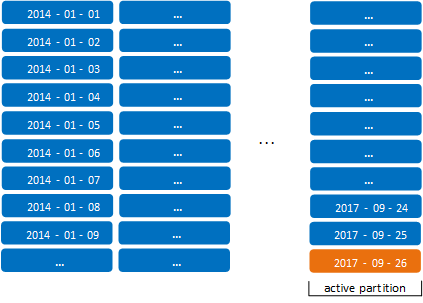
This is far above the recommended maximum of 50 partitions per projection. This number is also close to the default system limit of 1024 ROS containers per projection, risking ROS pushback in the near future.
You can approach this problem in several ways:
-
Consider consolidating table data into larger partitions—for example, partition by month instead of day. However, partitioning data at this level might limit effective use of partition management functions.
-
Regularly archive older partitions, and thereby minimize the number of accumulated partitions. However, this requires an extra layer of data management, and also inhibits access to historical data.
Alternatively, you can use CALENDAR_HIERARCHY_DAY to automatically merge partitions into a date-based hierarchy of partition groups. Each partition group is stored in its own set of ROS containers, apart from other groups. You specify this function in the table partition clause as follows:
PARTITION BY partition‑expression
GROUP BY CALENDAR_HIERARCHY_DAY( partition‑expression [, active‑months[, active‑years] ] )
Important
Two requirements apply to using CALENDAR_HIERARCHY_DAY in a partition clause:
For example, given the previous table, you can repartition it as follows:
=> ALTER TABLE public.store_orders
PARTITION BY order_date::DATE
GROUP BY CALENDAR_HIERARCHY_DAY(order_date::DATE, 2, 2) REORGANIZE;
Grouping DATE data hierarchically
CALENDAR_HIERARCHY_DAY creates hierarchies of partition groups, and merges partitions into the appropriate groups. It does so by evaluating the partition expression of each table row with the following algorithm, to determine its partition group key:
GROUP BY (
CASE WHEN DATEDIFF('YEAR', partition-expression, NOW()::TIMESTAMPTZ(6)) >= active-years
THEN DATE_TRUNC('YEAR', partition-expression::DATE)
WHEN DATEDIFF('MONTH', partition-expression, NOW()::TIMESTAMPTZ(6)) >= active-months
THEN DATE_TRUNC('MONTH', partition-expression::DATE)
ELSE DATE_TRUNC('DAY', partition-expression::DATE) END);
In this example, the algorithm compares order_date in each store_orders row to the current date as follows:
-
Determines whether order_date is in an inactive year.
If order_date is in an inactive year, the row's partition group key resolves to that year. The row is merged into a ROS container for that year.
-
If order_date is an active year, CALENDAR_HIERARCHY_DAY evaluates order_date to determine whether it is in an inactive month.
If order_date is in an inactive month, the row's partition group key resolves to that month. The row is merged into a ROS container for that month.
-
If order_date is in an active month, the row's partition group key resolves to the order_date day. This row is merged into a ROS container for that day. Any rows where order_date is a future date is treated in the same way.
Important
The CALENDAR_HIERARCHY_DAY algorithm assumes that most table activity is focused on recent dates. Setting active‑years and active‑months to a low number ≥ 2 serves to isolate most merge activity to date-specific containers, and incurs minimal overhead. Vertica recommends that you use the default setting of 2 for active‑years and active‑months. For most users, these settings achieve an optimal balance between ROS storage and performance.
As a best practice, never set active‑years and active‑months to 0.
For example, if the current date is 2017‑09-26, CALENDAR_HIERARCHY_DAY resolves active‑years and active‑months to the following date spans:
-
active‑years: 2016-01-01 to 2017-12-31. Partitions in active years are grouped into monthly ROS containers or are merged into daily ROS containers. Partitions from earlier years are regarded as inactive and merged into yearly ROS containers.
-
active‑months: 2017-08-01 to 2017-09-30. Partitions in active months are merged into daily ROS containers.
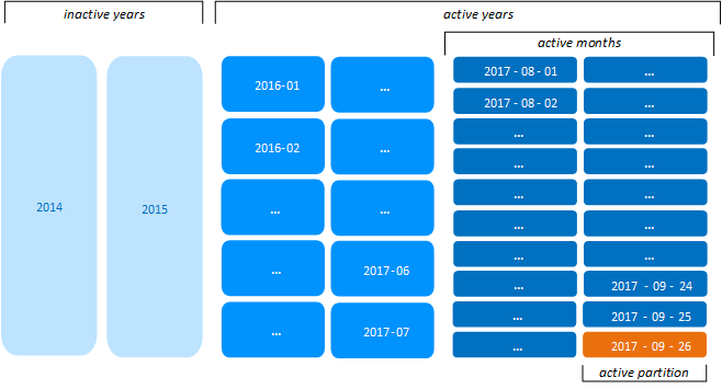
Now, the total number of ROS containers is reduced to 40 per projection:
=> SELECT COUNT (DISTINCT ros_id) NumROS, node_name FROM PARTITIONS
WHERE projection_name ilike '%store_orders_super%' GROUP BY node_name ORDER BY node_name;
NumROS | node_name
--------+------------------
40 | v_vmart_node0001
40 | v_vmart_node0002
40 | v_vmart_node0003
(3 rows)
Note
Regardless of how the Tuple Mover groups and merges partitions, it always identifies one or more partitions or partition groups as active. For details, see
Active and inactive partitions.
Dynamic regrouping
As shown earlier, CALENDAR_HIERARCHY_DAY references the current date when it creates partition group keys and merges partitions. As the calendar advances, the Tuple Mover reevaluates the partition group keys of tables that are partitioned with this function, and moves partitions as needed to different ROS containers.
Thus, given the previous example, on 2017-10-01 the Tuple Mover creates a monthly ROS container for August partitions. All partition keys between 2017-08-01 and 2017-08-31 are merged into the new ROS container 2017-08:
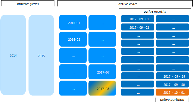
Likewise, on 2018-01-01, the Tuple Mover creates a ROS container for 2016 partitions. All partition keys between 2016-01-01 and 2016-12-31 that were previously grouped by month are merged into the new yearly ROS container:
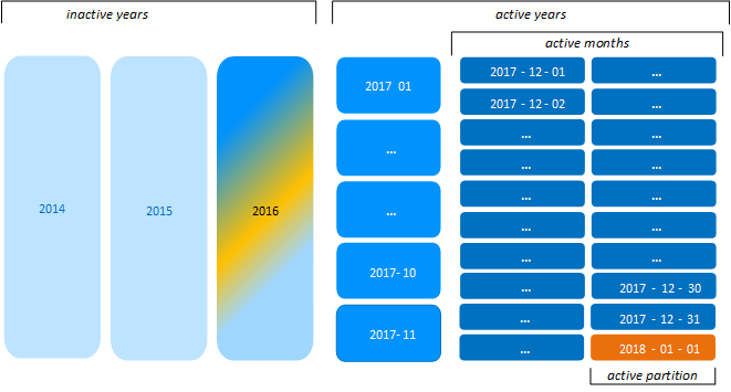
Caution
After older partitions are grouped into months and years, any partition operation that acts on a subset of older partition groups is liable to split ROS containers into smaller ROS containers for each partition—for example,
MOVE_PARTITIONS_TO_TABLE, where
force‑split is set to true. These operations can lead to ROS pushback. If you anticipate frequent partition operations on hierarchically grouped partitions,
consider modifying the partition expression so partitions are grouped no higher than months.
Customizing partition group hierarchies
Vertica provides a single function, CALENDAR_HIERARCHY_DAY, to facilitate hierarchical partitioning. Vertica stores the GROUP BY clause as a CASE statement that you can edit to suit your own requirements.
For example, Vertica stores the store_orders partition clause as follows:
=> ALTER TABLE public.store_orders
PARTITION BY order_date::DATE
GROUP BY CALENDAR_HIERARCHY_DAY(order_date::DATE, 2, 2);
=> select export_tables('','store_orders');
...
CREATE TABLE public.store_orders ( ... )
PARTITION BY ((store_orders.order_date)::date)
GROUP BY (
CASE WHEN ("datediff"('year', (store_orders.order_date)::date, ((now())::timestamptz(6))::date) >= 2)
THEN (date_trunc('year', (store_orders.order_date)::date))::date
WHEN ("datediff"('month', (store_orders.order_date)::date, ((now())::timestamptz(6))::date) >= 2)
THEN (date_trunc('month', (store_orders.order_date)::date))::date
ELSE (store_orders.order_date)::date END);
You can modify the CASE statement to customize the hierarchy of partition groups. For example, the following CASE statement creates a hierarchy of months, days, and hours:
=> ALTER TABLE store_orders
PARTITION BY (store_orders.order_date)
GROUP BY (
CASE WHEN DATEDIFF('MONTH', store_orders.order_date, NOW()::TIMESTAMPTZ(6)) >= 2
THEN DATE_TRUNC('MONTH', store_orders.order_date::DATE)
WHEN DATEDIFF('DAY', store_orders.order_date, NOW()::TIMESTAMPTZ(6)) >= 2
THEN DATE_TRUNC('DAY', store_orders.order_date::DATE)
ELSE DATE_TRUNC('hour', store_orders.order_date::DATE) END);
10.3 - Partitioning and segmentation
In Vertica, partitioning and segmentation are separate concepts and achieve different goals to localize data:.
In Vertica, partitioning and segmentation are separate concepts and achieve different goals to localize data:
-
Segmentation refers to organizing and distributing data across cluster nodes for fast data purges and query performance. Segmentation aims to distribute data evenly across multiple database nodes so all nodes participate in query execution. You specify segmentation with the
CREATE PROJECTION statement's hash segmentation clause.
-
Partitioning specifies how to organize data within individual nodes for distributed computing. Node partitions let you easily identify data you wish to drop and help reclaim disk space. You specify partitioning with the
CREATE TABLE statement's PARTITION BY clause.
For example: partitioning data by year makes sense for retaining and dropping annual data. However, segmenting the same data by year would be inefficient, because the node holding data for the current year would likely answer far more queries than the other nodes.
The following diagram illustrates the flow of segmentation and partitioning on a four-node database cluster:
-
Example table data
-
Data segmented by HASH(order_id)
-
Data segmented by hash across four nodes
-
Data partitioned by year on a single node
While partitioning occurs on all four nodes, the illustration shows partitioned data on one node for simplicity.
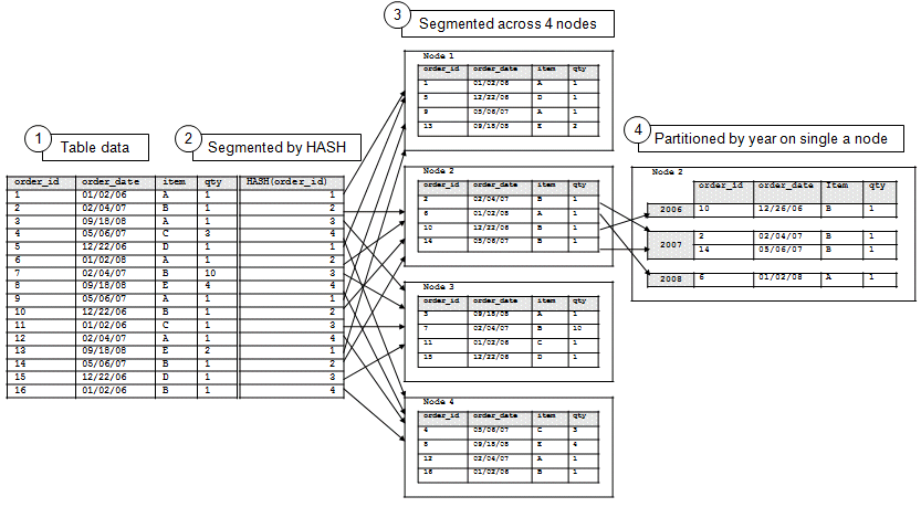
See also
10.4 - Managing partitions
You can manage partitions with the following operations:.
You can manage partitions with the following operations:
10.4.1 - Dropping partitions
Use the DROP_PARTITIONS function to drop one or more partition keys for a given table.
Use the DROP_PARTITIONS function to drop one or more partition keys for a given table. You can specify a single partition key or a range of partition keys.
For example, the table shown in Partitioning a new table is partitioned by column order_date:
=> CREATE TABLE public.store_orders
(
order_no int,
order_date timestamp NOT NULL,
shipper varchar(20),
ship_date date
)
PARTITION BY YEAR(order_date);
Given this table definition, Vertica creates a partition key for each unique order_date year—in this case, 2017, 2016, 2015, and 2014—and divides the data into separate ROS containers accordingly.
The following DROP_PARTITIONS statement drops from table store_orders all order records associated with partition key 2014:
=> SELECT DROP_PARTITIONS ('store_orders', 2014, 2014);
Partition dropped
Splitting partition groups
If a table partition clause includes a GROUP BY clause, partitions are consolidated in the ROS by their partition group keys. DROP_PARTITIONS can then specify a range of partition keys within a given partition group, or across multiple partition groups. In either case, the drop operation requires Vertica to split the ROS containers that store these partitions. To do so, the function's force_split parameter must be set to true.
For example, the store_orders table shown above can be repartitioned with a GROUP BY clause as follows:
=> ALTER TABLE store_orders
PARTITION BY order_date::DATE GROUP BY DATE_TRUNC('year', (order_date)::DATE) REORGANIZE;
With all 2014 order records having been dropped earlier, order_date values now span three years—2017, 2016, and 2015. Accordingly, the Tuple Mover creates three partition group keys for each year, and designates one or more ROS containers for each group. It then merges store_orders partitions into the appropriate groups.
The following DROP_PARTITIONS statement specifies to drop order dates that span two years, 2014 and 2015:
=> SELECT DROP_PARTITIONS('store_orders', '2015-05-30', '2016-01-16', 'true');
Partition dropped
The drop operation requires Vertica to drop partitions from two partition groups—2015 and 2016. These groups span at least two ROS containers, which must be split in order to remove the target partitions. Accordingly, the function's force_split parameter is set to true.
Scheduling partition drops
If your hardware has fixed disk space, you might need to configure a regular process to roll out old data by dropping partitions.
For example, if you have only enough space to store data for a fixed number of days, configure Vertica to drop the oldest partition keys. To do so, create a time-based job scheduler such as cron to schedule dropping the partition keys during low-load periods.
If the ingest rate for data has peaks and valleys, you can use two techniques to manage how you drop partition keys:
- Set up a process to check the disk space on a regular (daily) basis. If the percentage of used disk space exceeds a certain threshold—for example, 80%—drop the oldest partition keys.
- Add an artificial column in a partition that increments based on a metric like row count. For example, that column might increment each time the row count increases by 100 rows. Set up a process that queries this column on a regular (daily) basis. If the value in the new column exceeds a certain threshold—for example, 100—drop the oldest partition keys, and set the column value back to 0.
Table locking
DROP_PARTITIONS requires an exclusive D lock on the target table. This lock is only compatible with I-lock operations, so only table load operations such as INSERT and COPY are allowed during drop partition operations.
10.4.2 - Archiving partitions
You can move partitions from one table to another with the Vertica function MOVE_PARTITIONS_TO_TABLE.
You can move partitions from one table to another with the Vertica function
MOVE_PARTITIONS_TO_TABLE. This function is useful for archiving old partitions, as part of the following procedure:
-
Identify the partitions to archive, and move them to a temporary staging table with
MOVE_PARTITIONS_TO_TABLE.
-
Back up the staging table.
-
Drop the staging table.
You restore archived partitions at any time.
Move partitions to staging tables
You archive historical data by identifying the partitions you wish to remove from a table. You then move each partition (or group of partitions) to a temporary staging table.
Before calling MOVE_PARTITIONS_TO_TABLE:
- Refresh all out-of-date projections.
The following recommendations apply to staging tables:
-
To facilitate the backup process, create a unique schema for the staging table of each archiving operation.
-
Specify new names for staging tables. This ensures that they do not contain partitions from previous move operations.
If the table does not exist, Vertica creates a table from the source table's definition, by calling
CREATE TABLE with LIKE and INCLUDING PROJECTIONS clause. The new table inherits ownership from the source table. For details, see Replicating a table.
-
Use staging names that enable other users to easily identify partition contents. For example, if a table is partitioned by dates, use a name that specifies a date or date range.
In the following example, MOVE_PARTITIONS_TO_TABLE specifies to move a single partition to the staging table partn_backup.tradfes_200801.
=> SELECT MOVE_PARTITIONS_TO_TABLE (
'prod_trades',
'200801',
'200801',
'partn_backup.trades_200801');
MOVE_PARTITIONS_TO_TABLE
-------------------------------------------------
1 distinct partition values moved at epoch 15.
(1 row)
Back up the staging table
After you create a staging table, you archive it through an object-level backup using a
vbr configuration file. For detailed information, see Backing up and restoring the database.
Important
Vertica recommends performing a full database backup before the object-level backup, as a precaution against data loss. You can only restore object-level backups to the original database.
Drop the staging tables
After the backup is complete, you can drop the staging table as described in Dropping tables.
Restoring archived partitions
You can restore partitions that you previously moved to an intermediate table, archived as an object-level backup, and then dropped.
Note
Restoring an archived partition requires that the original table definition is unchanged since the partition was archived and dropped. If the table definition changed, you can restore an archived partition with INSERT...SELECT statements, which are not described here.
These are the steps to restoring archived partitions:
-
Restore the backup of the intermediate table you saved when you moved one or more partitions to archive (see Archiving partitions).
-
Move the restored partitions from the intermediate table to the original table.
-
Drop the intermediate table.
10.4.3 - Swapping partitions
SWAP_PARTITIONS_BETWEEN_TABLES combines the operations of DROP_PARTITIONS and MOVE_PARTITIONS_TO_TABLE as a single transaction.
SWAP_PARTITIONS_BETWEEN_TABLES combines the operations of DROP_PARTITIONS and MOVE_PARTITIONS_TO_TABLE as a single transaction. SWAP_PARTITIONS_BETWEEN_TABLES is useful if you regularly load partitioned data from one table into another and need to refresh partitions in the second table.
For example, you might have a table of revenue that is partitioned by date, and you routinely move data into it from a staging table. Occasionally, the staging table contains data for dates that are already in the target table. In this case, you must first remove partitions from the target table for those dates, then replace them with the corresponding partitions from the staging table. You can accomplish both tasks with a single call to SWAP_PARTITIONS_BETWEEN_TABLES.
By wrapping the drop and move operations within a single transaction, SWAP_PARTITIONS_BETWEEN_TABLES maintains integrity of the swapped data. If any task in the swap operation fails, the entire operation fails and is rolled back.
Example
The following example creates two partitioned tables and then swaps certain partitions between them.
Both tables have the same definition and have partitions for various year values. You swap the partitions where year = 2008 and year = 2009. Both tables have at least two rows to swap.
-
Create the customer_info table:
=> CREATE TABLE customer_info (
customer_id INT NOT NULL,
first_name VARCHAR(25),
last_name VARCHAR(35),
city VARCHAR(25),
year INT NOT NULL)
ORDER BY last_name
PARTITION BY year;
-
Insert data into the customer_info table:
INSERT INTO customer_info VALUES
(1,'Joe','Smith','Denver',2008),
(2,'Bob','Jones','Boston',2008),
(3,'Silke','Muller','Frankfurt',2007),
(4,'Simone','Bernard','Paris',2014),
(5,'Vijay','Kumar','New Delhi',2010);
OUTPUT
--------
5
(1 row)
=> COMMIT;
-
View the table data:
=> SELECT * FROM customer_info ORDER BY year DESC;
customer_id | first_name | last_name | city | year
-------------+------------+-----------+-----------+------
4 | Simone | Bernard | Paris | 2014
5 | Vijay | Kumar | New Delhi | 2010
2 | Bob | Jones | Boston | 2008
1 | Joe | Smith | Denver | 2008
3 | Silke | Muller | Frankfurt | 2007
(5 rows)
-
Create a second table, member_info, that has the same definition as customer_info:
=> CREATE TABLE member_info LIKE customer_info INCLUDING PROJECTIONS;
CREATE TABLE
-
Insert data into the member_info table:
=> INSERT INTO member_info VALUES
(1,'Jane','Doe','Miami',2001),
(2,'Mike','Brown','Chicago',2014),
(3,'Patrick','OMalley','Dublin',2008),
(4,'Ana','Lopez','Madrid',2009),
(5,'Mike','Green','New York',2008);
OUTPUT
--------
5
(1 row)
=> COMMIT;
COMMIT
-
View the data in the member_info table:
=> SELECT * FROM member_info ORDER BY year DESC;
customer_id | first_name | last_name | city | year
-------------+------------+-----------+----------+------
2 | Mike | Brown | Chicago | 2014
4 | Ana | Lopez | Madrid | 2009
5 | Mike | Green | New York | 2008
3 | Patrick | OMalley | Dublin | 2008
1 | Jane | Doe | Miami | 2001
(5 rows)
-
To swap the partitions, run the SWAP_PARTITIONS_BETWEEN_TABLES function:
=> SELECT SWAP_PARTITIONS_BETWEEN_TABLES('customer_info', 2008, 2009, 'member_info');
SWAP_PARTITIONS_BETWEEN_TABLES
----------------------------------------------------------------------------------------------
1 partition values from table customer_info and 2 partition values from table member_info are swapped at epoch 1045.
(1 row)
-
Query both tables to confirm that they swapped their respective 2008 and 2009 records:
=> SELECT * FROM customer_info ORDER BY year DESC;
customer_id | first_name | last_name | city | year
-------------+------------+-----------+-----------+------
4 | Simone | Bernard | Paris | 2014
5 | Vijay | Kumar | New Delhi | 2010
4 | Ana | Lopez | Madrid | 2009
3 | Patrick | OMalley | Dublin | 2008
5 | Mike | Green | New York | 2008
3 | Silke | Muller | Frankfurt | 2007
(6 rows)
=> SELECT * FROM member_info ORDER BY year DESC;
customer_id | first_name | last_name | city | year
-------------+------------+-----------+---------+------
2 | Mike | Brown | Chicago | 2014
2 | Bob | Jones | Boston | 2008
1 | Joe | Smith | Denver | 2008
1 | Jane | Doe | Miami | 2001
(4 rows)
10.4.4 - Minimizing partitions
By default, Vertica supports up to 1024 ROS containers to store partitions for a given projection (see Projection Parameters).
By default, Vertica supports up to 1024 ROS containers to store partitions for a given projection (see Projection parameters). A ROS container contains data that share the same partition key, or the same partition group key. Depending on the amount of data per partition, a partition or partition group can span multiple ROS containers.
Given this limit, it is inadvisable to partition a table on highly granular data—for example, on a TIMESTAMP column. Doing so can generate a very high number of partitions. If the number of partitions requires more than 1024 ROS containers, Vertica issues a ROS pushback warning and refuses to load more table data. A large number of ROS containers also can adversely affect DML operations such as DELETE, which requires Vertica to open all ROS containers.
In practice, it is unlikely you will approach this maximum. For optimal performance, Vertica recommends that the number of ungrouped partitions range between 10 and 20, and not exceed 50. This range is typically compatible with most business requirements.
You can also reduce the number of ROS containers by grouping partitions. For more information, see Partition grouping and Hierarchical partitioning.
10.4.5 - Viewing partition storage data
Vertica provides various ways to view how your table partitions are organized and stored:.
Vertica provides various ways to view how your table partitions are organized and stored:
Querying PARTITIONS table
The following table and projection definitions partition store_order data on order dates, and groups together partitions of the same year:
=> CREATE TABLE public.store_orders
(order_no int, order_date timestamp NOT NULL, shipper varchar(20), ship_date date)
PARTITION BY ((order_date)::date) GROUP BY (date_trunc('year', (order_date)::date));
=> CREATE PROJECTION public.store_orders_super
AS SELECT order_no, order_date, shipper, ship_date FROM store_orders
ORDER BY order_no, order_date, shipper, ship_date UNSEGMENTED ALL NODES;
=> COPY store_orders FROM '/home/dbadmin/export_store_orders_data.txt';
After loading data into this table, you can query the PARTITIONS table to determine how many ROS containers store the grouped partitions for projection store_orders_unseg, across all nodes. Each node has eight ROS containers, each container storing partitions of one partition group:
=> SELECT COUNT (partition_key) NumPartitions, ros_id, node_name FROM PARTITIONS
WHERE projection_name ilike 'store_orders%' GROUP BY ros_id, node_name ORDER BY node_name, NumPartitions;
NumPartitions | ros_id | node_name
---------------+-------------------+------------------
173 | 45035996274562779 | v_vmart_node0001
211 | 45035996274562791 | v_vmart_node0001
212 | 45035996274562783 | v_vmart_node0001
213 | 45035996274562787 | v_vmart_node0001
173 | 49539595901916471 | v_vmart_node0002
211 | 49539595901916483 | v_vmart_node0002
212 | 49539595901916475 | v_vmart_node0002
213 | 49539595901916479 | v_vmart_node0002
173 | 54043195529286985 | v_vmart_node0003
211 | 54043195529286997 | v_vmart_node0003
212 | 54043195529286989 | v_vmart_node0003
213 | 54043195529286993 | v_vmart_node0003
(12 rows)
Dumping partition keys
Vertica provides several functions that let you inspect how individual partitions are stored on the cluster, at several levels:
Given the previous table and projection, DUMP_PROJECTION_PARTITION_KEYS shows the contents of four ROS containers on each node:
=> SELECT DUMP_PROJECTION_PARTITION_KEYS('store_orders_super');
...
Partition keys on node v_vmart_node0001
Projection 'store_orders_super'
Storage [ROS container]
No of partition keys: 173
Partition keys: 2017-01-02 2017-01-03 2017-01-04 2017-01-05 2017-01-06 2017-01-09 2017-01-10
2017-01-11 2017-01-12 2017-01-13 2017-01-16 2017-01-17 2017-01-18 2017-01-19 2017-01-20 2017-01-23
2017-01-24 2017-01-25 2017-01-26 2017-01-27 2017-02-01 2017-02-02 2017-02-03 2017-02-06 2017-02-07
2017-02-08 2017-02-09 2017-02-10 2017-02-13 2017-02-14 2017-02-15 2017-02-16 2017-02-17 2017-02-20
...
2017-09-01 2017-09-04 2017-09-05 2017-09-06 2017-09-07 2017-09-08 2017-09-11 2017-09-12 2017-09-13
2017-09-14 2017-09-15 2017-09-18 2017-09-19 2017-09-20 2017-09-21 2017-09-22 2017-09-25 2017-09-26 2017-09-27
Storage [ROS container]
No of partition keys: 212
Partition keys: 2016-01-01 2016-01-04 2016-01-05 2016-01-06 2016-01-07 2016-01-08 2016-01-11
2016-01-12 2016-01-13 2016-01-14 2016-01-15 2016-01-18 2016-01-19 2016-01-20 2016-01-21 2016-01-22
2016-01-25 2016-01-26 2016-01-27 2016-02-01 2016-02-02 2016-02-03 2016-02-04 2016-02-05 2016-02-08
2016-02-09 2016-02-10 2016-02-11 2016-02-12 2016-02-15 2016-02-16 2016-02-17 2016-02-18 2016-02-19
...
2016-11-01 2016-11-02 2016-11-03 2016-11-04 2016-11-07 2016-11-08 2016-11-09 2016-11-10 2016-11-11
2016-11-14 2016-11-15 2016-11-16 2016-11-17 2016-11-18 2016-11-21 2016-11-22 2016-11-23 2016-11-24 2016-11-25
Storage [ROS container]
No of partition keys: 213
Partition keys: 2015-01-01 2015-01-02 2015-01-05 2015-01-06 2015-01-07 2015-01-08 2015-01-09
2015-01-12 2015-01-13 2015-01-14 2015-01-15 2015-01-16 2015-01-19 2015-01-20 2015-01-21 2015-01-22
2015-01-23 2015-01-26 2015-01-27 2015-02-02 2015-02-03 2015-02-04 2015-02-05 2015-02-06 2015-02-09
2015-02-10 2015-02-11 2015-02-12 2015-02-13 2015-02-16 2015-02-17 2015-02-18 2015-02-19 2015-02-20
...
2015-11-02 2015-11-03 2015-11-04 2015-11-05 2015-11-06 2015-11-09 2015-11-10 2015-11-11 2015-11-12
2015-11-13 2015-11-16 2015-11-17 2015-11-18 2015-11-19 2015-11-20 2015-11-23 2015-11-24 2015-11-25
2015-11-26 2015-11-27
Storage [ROS container]
No of partition keys: 211
Partition keys: 2014-01-01 2014-01-02 2014-01-03 2014-01-06 2014-01-07 2014-01-08 2014-01-09
2014-01-10 2014-01-13 2014-01-14 2014-01-15 2014-01-16 2014-01-17 2014-01-20 2014-01-21 2014-01-22
2014-01-23 2014-01-24 2014-01-27 2014-02-03 2014-02-04 2014-02-05 2014-02-06 2014-02-07 2014-02-10
2014-02-11 2014-02-12 2014-02-13 2014-02-14 2014-02-17 2014-02-18 2014-02-19 2014-02-20 2014-02-21
...
2014-11-04 2014-11-05 2014-11-06 2014-11-07 2014-11-10 2014-11-11 2014-11-12 2014-11-13 2014-11-14
2014-11-17 2014-11-18 2014-11-19 2014-11-20 2014-11-21 2014-11-24 2014-11-25 2014-11-26 2014-11-27
Storage [ROS container]
No of partition keys: 173
...
10.5 - Active and inactive partitions
Partitioned tables in the same database can be subject to different distributions of update and load activity.
The Tuple Mover assumes that all loads and updates to a partitioned table are targeted to one or more partitions that it identifies as active. In general, the partitions with the largest partition keys—typically, the most recently created partitions—are regarded as active. As the partition ages, its workload typically shrinks and becomes mostly read-only.
Setting active partition count
You can specify how many partitions are active for partitioned tables at two levels, in ascending order of precedence:
-
Configuration parameter ActivePartitionCount determines how many partitions are active for partitioned tables in the database. By default, ActivePartitionCount is set to 1. The Tuple Mover applies this setting to all tables that do not set their own active partition count.
-
Individual tables can supersede ActivePartitionCount by setting their own active partition count with CREATE TABLE and ALTER TABLE.
Partitioned tables in the same database can be subject to different distributions of update and load activity. When these differences are significant, it might make sense for some tables to set their own active partition counts.
For example, table store_orders is partitioned by month and gets its active partition count from configuration parameter ActivePartitionCount. If the parameter is set to 1, the Tuple Mover identifes the latest month—typically, the current one—as the table's active partition. If store_orders is subject to frequent activity on data for the current month and the one before it, you might want the table to supersede the configuration parameter, and set its active partition count to 2:
ALTER TABLE public.store_orders SET ACTIVEPARTITIONCOUNT 2;
Note
For tables partitioned by non-temporal attributes, set its active partition count to reflect the number of partitions that are subject to a high level of activity—for example, frequent loads or queries.
Identifying the active partition
The Tuple Mover typically identifies the active partition as the one most recently created. Vertica uses the following algorithm to determine which partitions are older than others:
-
If partition X was created before partition Y, partition X is older.
-
If partitions X and Y were created at the same time, but partition X was last updated before partition Y, partition X is older.
-
If partitions X and Y were created and last updated at the same time, the partition with the smaller key is older.
You can obtain the active partitions for a table by joining system tables
PARTITIONS and
STRATA and querying on its projections. For example, the following query gets the active partition for projection store_orders_super:
=> SELECT p.node_name, p.partition_key, p.ros_id, p.ros_size_bytes, p.ros_row_count, ROS_container_count
FROM partitions p JOIN strata s ON p.partition_key = s.stratum_key AND p.node_name=s.node_name
WHERE p.projection_name = 'store_orders_super' ORDER BY p.node_name, p.partition_key;
node_name | partition_key | ros_id | ros_size_bytes | ros_row_count | ROS_container_count
------------------+---------------+-------------------+----------------+---------------+---------------------
v_vmart_node0001 | 2017-09-01 | 45035996279322851 | 6905 | 960 | 1
v_vmart_node0002 | 2017-09-01 | 49539595906590663 | 6905 | 960 | 1
v_vmart_node0003 | 2017-09-01 | 54043195533961159 | 6905 | 960 | 1
(3 rows)
Active partition groups
If a table's partition clause includes a GROUP BY expression, Vertica applies the table's active partition count to its largest partition group key, and regards all the partitions in that group as active. If you group partitions with Vertica meta-function
CALENDAR_HIERARCHY_DAY, the most recent date partitions are also grouped by day. Thus, the largest partition group key and largest partition key are identical. In effect, this means that only the most recent partitions are active.
For more information about partition grouping, see Partition grouping and Hierarchical partitioning.
10.6 - Partition pruning
If a query predicate specifies a partitioning expression, the query optimizer evaluates the predicate against the containers of the partitioned data.
If a query predicate specifies a partitioning expression, the query optimizer evaluates the predicate against the ROS containers of the partitioned data. Each ROS container maintains the minimum and maximum values of its partition key data. The query optimizer uses this metadata to determine which ROS containers it needs to execute the query, and omits, or prunes, the remaining containers from the query plan. By minimizing the number of ROS containers that it must scan, the query optimizer enables faster execution of the query.
For example, a table might be partitioned by year as follows:
=> CREATE TABLE ... PARTITION BY EXTRACT(year FROM date);
Given this table definition, its projection data is partitioned into ROS containers according to year, one for each year—in this case, 2007, 2008, 2009.
The following query specifies the partition expression date:
=> SELECT ... WHERE date = '12-2-2009';
Given this query, the ROS containers that contain data for 2007 and 2008 fall outside the boundaries of the requested year (2009). The query optimizer prunes these containers from the query plan before the query executes:
Examples
Assume a table that is partitioned by time and will use queries that restrict data on time.
=> CREATE TABLE time ( tdate DATE NOT NULL, tnum INTEGER)
PARTITION BY EXTRACT(year FROM tdate);
=> CREATE PROJECTION time_p (tdate, tnum) AS
=> SELECT * FROM time ORDER BY tdate, tnum UNSEGMENTED ALL NODES;
Note
Projection sort order has no effect on partition pruning.
=> INSERT INTO time VALUES ('03/15/04' , 1);
=> INSERT INTO time VALUES ('03/15/05' , 2);
=> INSERT INTO time VALUES ('03/15/06' , 3);
=> INSERT INTO time VALUES ('03/15/06' , 4);
The data inserted in the previous series of commands are loaded into three ROS containers, one per year, as that is how the data is partitioned:
=> SELECT * FROM time ORDER BY tnum;
tdate | tnum
------------+------
2004-03-15 | 1 --ROS1 (min 03/01/04, max 03/15/04)
2005-03-15 | 2 --ROS2 (min 03/15/05, max 03/15/05)
2006-03-15 | 3 --ROS3 (min 03/15/06, max 03/15/06)
2006-03-15 | 4 --ROS3 (min 03/15/06, max 03/15/06)
(4 rows)
Here's what happens when you query the time table:
-
In this query, Vertica can omit container ROS2 because it is only looking for year 2004:
=> SELECT COUNT(*) FROM time WHERE tdate = '05/07/2004';
-
In the next query, Vertica can omit two containers, ROS1 and ROS3:
=> SELECT COUNT(*) FROM time WHERE tdate = '10/07/2005';
-
The following query has an additional predicate on the tnum column for which no minimum/maximum values are maintained. In addition, the use of logical operator OR is not supported, so no ROS elimination occurs:
=> SELECT COUNT(*) FROM time WHERE tdate = '05/07/2004' OR tnum = 7;
11 - Constraints
Constraints set rules on what data is allowed in table columns.
Constraints set rules on what data is allowed in table columns. Using constraints can help maintain data integrity. For example, you can constrain a column to allow only unique values, or to disallow NULL values. Constraints such as primary keys also help the optimizer generate query plans that facilitate faster data access, particularly for joins.
You set constraints on a new table and an existing one with
CREATE TABLE and
ALTER TABLE...ADD CONSTRAINT, respectively.
11.1 - Supported constraints
Vertica supports standard SQL constraints, as described in this section.
Vertica supports standard SQL constraints, as described in this section.
11.1.1 - Primary key constraints
A primary key comprises one or multiple columns of primitive types, whose values can uniquely identify table rows.
A primary key comprises one or multiple columns of primitive types, whose values can uniquely identify table rows. A table can specify only one primary key. You identify a table's primary key when you create the table, or in an existing table with
ALTER TABLE. You cannot designate a column with a collection type as a key.
For example, the following CREATE TABLE statement defines the order_no column as the primary key of the store_orders table:
=> CREATE TABLE public.store_orders(
order_no int PRIMARY KEY,
order_date timestamp NOT NULL,
shipper varchar(20),
ship_date date,
product_key int,
product_version int
)
PARTITION BY ((date_part('year', order_date))::int);
CREATE TABLE
Multi-column primary keys
A primary key can comprise multiple columns. In this case, the CREATE TABLE statement must specify the constraint after all columns are defined, as follows:
=> CREATE TABLE public.product_dimension(
product_key int,
product_version int,
product_description varchar(128),
sku_number char(32) UNIQUE,
category_description char(32),
CONSTRAINT pk PRIMARY KEY (product_key, product_version) ENABLED
);
CREATE TABLE
Alternatively, you can specify the table's primary key with a separate
ALTER TABLE...ADD CONSTRAINT statement, as follows:
=> ALTER TABLE product_dimension ADD CONSTRAINT pk PRIMARY KEY (product_key, product_version) ENABLED;
ALTER TABLE
Enforcing primary keys
You can prevent loading duplicate values into primary keys by enforcing the primary key constraint. Doing so allows you to join tables on their primary and foreign keys. When a query joins a dimension table to a fact table, each primary key in the dimension table must uniquely match each foreign key value in the fact table. Otherwise, attempts to join these tables return a key enforcement error.
You enforce primary key constraints globally with configuration parameter EnableNewPrimaryKeysByDefault. You can also enforce primary key constraints for specific tables by qualifying the constraint with the keyword ENABLED. In both cases, Vertica checks key values as they are loaded into tables, and returns errors on any constraint violations. Alternatively, use
ANALYZE_CONSTRAINTS to validate primary keys after updating table contents. For details, see Constraint enforcement.
Tip
Consider using
sequences for primary key columns to guarantee uniqueness, and avoid the resource overhead that primary key constraints can incur.
Setting NOT NULL on primary keys
When you define a primary key , Vertica automatically sets the primary key columns to NOT NULL. For example, when you create the table product_dimension as shown earlier, Vertica sets primary key columns product_key and product_version to NOT NULL, and stores them in the catalog accordingly:
> SELECT EXPORT_TABLES('','product_dimension');
...
CREATE TABLE public.product_dimension
(
product_key int NOT NULL,
product_version int NOT NULL,
product_description varchar(128),
sku_number char(32),
category_description char(32),
CONSTRAINT C_UNIQUE UNIQUE (sku_number) DISABLED,
CONSTRAINT pk PRIMARY KEY (product_key, product_version) ENABLED
);
(1 row)
If you specify a primary key for an existing table with ALTER TABLE, Vertica notifies you that it set the primary key columns to NOT NULL:
WARNING 2623: Column "column-name" definition changed to NOT NULL
Note
If you drop a primary key constraint, the columns that comprised it remain set to
NOT NULL. This constraint can only be removed explicitly, through
ALTER TABLE...ALTER COLUMN.
11.1.2 - Foreign key constraints
A foreign key joins a table to another table by referencing its primary key.
A foreign key joins a table to another table by referencing its primary key. A foreign key constraint specifies that the key can only contain values that are in the referenced primary key, and thus ensures the referential integrity of data that is joined on the two keys.
You can identify a table's foreign key when you create the table, or in an existing table with
ALTER TABLE. For example, the following CREATE TABLE statement defines two foreign key constraints: fk_store_orders_store and fk_store_orders_vendor:
=> CREATE TABLE store.store_orders_fact(
product_key int NOT NULL,
product_version int NOT NULL,
store_key int NOT NULL CONSTRAINT fk_store_orders_store REFERENCES store.store_dimension (store_key),
vendor_key int NOT NULL CONSTRAINT fk_store_orders_vendor REFERENCES public.vendor_dimension (vendor_key),
employee_key int NOT NULL,
order_number int NOT NULL,
date_ordered date,
date_shipped date,
expected_delivery_date date,
date_delivered date,
quantity_ordered int,
quantity_delivered int,
shipper_name varchar(32),
unit_price int,
shipping_cost int,
total_order_cost int,
quantity_in_stock int,
reorder_level int,
overstock_ceiling int
);
The following ALTER TABLE statement adds foreign key constraint fk_store_orders_employee to the same table:
=> ALTER TABLE store.store_orders_fact ADD CONSTRAINT fk_store_orders_employee
FOREIGN KEY (employee_key) REFERENCES public.employee_dimension (employee_key);
The REFERENCES clause can omit the name of the referenced column if it is the same as the foreign key column name. For example, the following ALTER TABLE statement is equivalent to the one above:
=> ALTER TABLE store.store_orders_fact ADD CONSTRAINT fk_store_orders_employee
FOREIGN KEY (employee_key) REFERENCES public.employee_dimension;
Multi-column foreign keys
If a foreign key refrences a primary key that contains multiple columns, the foreign key must contain the same number of columns. For example, the primary key for table public.product_dimension contains two columns, product_key and product_version. In this case, CREATE TABLE can define a foreign key constraint that references this primary key as follows:
=> CREATE TABLE store.store_orders_fact3(
product_key int NOT NULL,
product_version int NOT NULL,
...
CONSTRAINT fk_store_orders_product
FOREIGN KEY (product_key, product_version) REFERENCES public.product_dimension (product_key, product_version)
);
CREATE TABLE
CREATE TABLE can specify multi-column foreign keys only after all table columns are defined. You can also specify the table's foreign key with a separate
ALTER TABLE...ADD CONSTRAINT statement:
=> ALTER TABLE store.store_orders_fact ADD CONSTRAINT fk_store_orders_product
FOREIGN KEY (product_key, product_version) REFERENCES public.product_dimension (product_key, product_version);
In both examples, the constraint specifies the columns in the referenced table. If the referenced column names are the same as the foreign key column names, the REFERENCES clause can omit them. For example, the following ALTER TABLE statement is equivalent to the previous one:
=> ALTER TABLE store.store_orders_fact ADD CONSTRAINT fk_store_orders_product
FOREIGN KEY (product_key, product_version) REFERENCES public.product_dimension;
NULL values in foreign key
A foreign key that whose columns omit NOT NULL can contain NULL values, even if the primary key contains no NULL values. Thus, you can insert rows into the table even if their foreign key is not yet known.
11.1.3 - Unique constraints
You can specify a unique constraint on a column so each value in that column is unique among all other values.
You can specify a unique constraint on a column so each value in that column is unique among all other values. You can define a unique constraint when you create a table, or you can add a unique constraint to an existing table with
ALTER TABLE. You cannot use a uniqueness constraint on a column with a collection type.
For example, the following ALTER TABLE statement defines the sku_number column in the product_dimensions table as unique:
=> ALTER TABLE public.product_dimension ADD UNIQUE(sku_number);
WARNING 4887: Table product_dimension has data. Queries using this table may give wrong results
if the data does not satisfy this constraint
HINT: Use analyze_constraints() to check constraint violation on data
Enforcing unique constraints
You enforce unique constraints globally with configuration parameter EnableNewUniqueKeysByDefault. You can also enforce unique constraints for specific tables by qualifying their unique constraints with the keyword ENABLED. In both cases, Vertica checks values as they are loaded into unique columns, and returns with errors on any constraint violations. Alternatively, you can use
ANALYZE_CONSTRAINTS to validate unique constraints after updating table contents. For details, see Constraint enforcement.
For example, the previous example does not enforce the unique constraint in column sku_number. The following statement enables this constraint:
=> ALTER TABLE public.product_dimension ALTER CONSTRAINT C_UNIQUE ENABLED;
ALTER TABLE
Multi-column unique constraints
You can define a unique constraint that is comprised of multiple columns. The following CREATE TABLE statement specifies that the combined values of columns c1 and c2 in each row must be unique among all other rows:
CREATE TABLE dim1 (c1 INTEGER,
c2 INTEGER,
c3 INTEGER,
UNIQUE (c1, c2) ENABLED
);
11.1.4 - Check constraints
A check constraint specifies a Boolean expression that evaluates a column's value on each row.
A check constraint specifies a Boolean expression that evaluates a column's value on each row. If the expression resolves to false for a given row, the column value is regarded as violating the constraint.
For example, the following table specifies two named check constraints:
CREATE TABLE public.store_orders_2018 (
order_no int CONSTRAINT pk PRIMARY KEY,
product_key int,
product_version int,
order_date timestamp NOT NULL,
shipper varchar(20),
ship_date date,
CONSTRAINT IsYear2018 CHECK (DATE_PART('year', order_date)::int = 2018),
CONSTRAINT Ship5dAfterOrder CHECK (DAYOFYEAR(ship_date) - DAYOFYEAR(order_date) <=5)
);
When Vertica checks the data in store_orders_2018 for constraint violations, it evaluates the values of order_date and ship_date on each row, to determine whether they comply with their respective check constraints.
Check expressions
A check expression can only reference the current table row; it cannot access data stored in other tables or database objects, such as sequences. It also cannot access data in other table rows.
A check constraint expression can include:
-
Arithmetic and concatenated string operators
-
Logical operators such as AND, OR, NOT
-
WHERE prepositions such as CASE, IN, LIKE, BETWEEN, IS [NOT] NULL
-
Calls to the following function types:
Example check expressions
The following check expressions assume that the table contains all referenced columns and that they have the appropriate data types:
-
CONSTRAINT chk_pos_quant CHECK (quantity > 0)
-
CONSTRAINT chk_pqe CHECK (price*quantity = extended_price)
-
CONSTRAINT size_sml CHECK (size in ('s', 'm', 'l', 'xl'))
-
CHECK ( regexp_like(dept_name, '^[a-z]+$', 'i') OR (dept_name = 'inside sales'))
Check expression restrictions
A check expression must evaluate to a Boolean value. However, Vertica does not support implicit conversions to Boolean values. For example, the following check expressions are invalid:
-
CHECK (1)
-
CHECK ('hello')
A check expression cannot include the following elements:
-
Subqueries—for example, CHECK (dept_id in (SELECT id FROM dept))
-
Aggregates—for example, CHECK (quantity < sum(quantity)/2)
-
Window functions—for example, CHECK (RANK() over () < 3)
-
SQL meta-functions—for example, CHECK (START_REFRESH('') = 0)
-
References to the epoch column
-
References to other tables or objects (for example, sequences), or system context
-
Invocation of functions that are not immutable in time and space
Enforcing check constraints
You can enforce check constraints globally with configuration parameter EnableNewCheckConstraintsByDefault. You an also enforce check constraints for specific tables by qualifying unique constraints with the keyword ENABLED. In both cases, Vertica evaluates check constraints as new values are loaded into the table, and returns with errors on any constraint violations. Alternatively, you can use
ANALYZE_CONSTRAINTS to validate check constraints after updating the table contents. For details, see Constraint enforcement.
For example, you can enable the constraints shown earlier with ALTER TABLE...ALTER CONSTRAINT:
=> ALTER TABLE store_orders_2018 ALTER CONSTRAINT IsYear2018 ENABLED;
ALTER TABLE
=> ALTER TABLE store_orders_2018 ALTER CONSTRAINT Ship5dAfterOrder ENABLED;
ALTER TABLE
Check constraints and nulls
If a check expression evaluates to unknown for a given row because a column within the expression contains a null, the row passes the constraint condition. Vertica evaluates the expression and considers it satisfied if it resolves to either true or unknown. For example, check (quantity > 0) passes validation if quantity is null. This result differs from how a WHERE clause works. With a WHERE clause, the row would not be included in the result set.
You can prohibit nulls in a check constraint by explicitly including a null check in the check constraint expression. For example: CHECK (quantity IS NOT NULL AND (quantity > 0))
Tip
Alternatively, set a NOT NULL constraint on the same column.
Check constraints and SQL macros
A check constraint can call a SQL macro (a function written in SQL) if the macro is immutable. An immutable macro always returns the same value for a given set of arguments.
When a DDL statement specifies a macro in a check expression, Vertica determines if it is immutable. If it is not, Vertica rolls back the statement.
The following example creates the macro mycompute and then uses it in a check expression:
=> CREATE OR REPLACE FUNCTION mycompute(j int, name1 varchar)
RETURN int AS BEGIN RETURN (j + length(name1)); END;
=> ALTER TABLE sampletable
ADD CONSTRAINT chk_compute
CHECK(mycompute(weekly_hours, name1))<50);
Check constraints and UDSFs
A check constraint can call user-defined scalar functions (UDSFs). The following requirements apply:
Caution
Vertica evaluates an enabled check constraint on every row that is loaded or updated. Invoking a computationally expensive check constraint on a large table is liable to incur considerable system overhead.
For a usage example, see C++ example: calling a UDSF from a check constraint.
11.1.5 - NOT NULL constraints
A NOT NULL constraint specifies that a column cannot contain a null value.
A NOT NULL constraint specifies that a column cannot contain a null value. All table updates must specify values in columns with this constraint. You can set a NOT NULL constraint on columns when you create a table, or set the constraint on an existing table with ALTER TABLE.
The following CREATE TABLE statement defines three columns as NOT NULL. You cannot store any NULL values in those columns.
=> CREATE TABLE inventory ( date_key INTEGER NOT NULL,
product_key INTEGER NOT NULL,
warehouse_key INTEGER NOT NULL, ... );
The following ALTER TABLE statement defines column sku_number in table product_dimensions as NOT NULL:
=> ALTER TABLE public.product_dimension ALTER COLUMN sku_number SET NOT NULL;
ALTER TABLE
Enforcing NOT NULL constraints
You cannot enable enforcement of a NOT NULL constraint. You must use ANALYZE_CONSTRAINTS to determine whether column data contains null values, and then manually fix any constraint violations that the function finds.
NOT NULL and primary keys
When you define a primary key, Vertica automatically sets the primary key columns to NOT NULL. If you drop a primary key constraint, the columns that comprised it remain set to NOT NULL. This constraint can only be removed explicitly, through ALTER TABLE...ALTER COLUMN.
11.2 - Setting constraints
You can set constraints on a new table and an existing one with CREATE TABLE and ALTER TABLE...ADD CONSTRAINT, respectively.
You can set constraints on a new table and an existing one with
CREATE TABLE and
ALTER TABLE...ADD CONSTRAINT, respectively.
Setting constraints on a new table
CREATE TABLE can specify a constraint in two ways: as part of the column definition, or following all column definitions.
For example, the following CREATE TABLE statement sets two constraints on column sku_number, NOT NULL and UNIQUE. After all columns are defined, the statement also sets a primary key that is composed of two columns, product_key and product_version:
=> CREATE TABLE public.prod_dimension(
product_key int,
product_version int,
product_description varchar(128),
sku_number char(32) NOT NULL UNIQUE,
category_description char(32),
CONSTRAINT pk PRIMARY KEY (product_key, product_version) ENABLED
);
CREATE TABLE
Setting constraints on an existing table
ALTER TABLE...ADD CONSTRAINT adds a constraint to an existing table. For example, the following statement specifies unique values for column product_version:
=> ALTER TABLE prod_dimension ADD CONSTRAINT u_product_versions UNIQUE (product_version) ENABLED;
ALTER TABLE
Validating existing data
When you add a constraint on a column that already contains data, Vertica immediately validates column values if the following conditions are both true:
If either of these conditions is not true, Vertica does not validate the column values. In this case, you must call
ANALYZE_CONSTRAINTS to find constraint violations. Otherwise, queries are liable to return unexpected results. For details, see Detecting constraint violations.
Exporting table constraints
Whether you specify constraints in the column definition or on the table, Vertica stores the table DDL as part of the CREATE statement and exports them as such. One exception applies: foreign keys are stored and exported as ALTER TABLE statements.
For example:
=> SELECT EXPORT_TABLES('','prod_dimension');
...
CREATE TABLE public.prod_dimension
(
product_key int NOT NULL,
product_version int NOT NULL,
product_description varchar(128),
sku_number char(32) NOT NULL,
category_description char(32),
CONSTRAINT C_UNIQUE UNIQUE (sku_number) DISABLED,
CONSTRAINT pk PRIMARY KEY (product_key, product_version) ENABLED,
CONSTRAINT u_product_versions UNIQUE (product_version) ENABLED
);
(1 row)
11.3 - Dropping constraints
ALTER TABLE drops constraints from tables in two ways:.
ALTER TABLE drops constraints from tables in two ways:
For example, table store_orders_2018 specifies the following constraints:
-
Named constraint pk identifies column order_no as a primary key.
-
Named constraint IsYear2018 specifies a check constraint that allows only 2018 dates in column order_date.
-
Named constraint Ship5dAfterOrder specifies a check constraint that disallows any ship_date value that is more than 5 days after order_date.
-
Columns order_no and order_date are set to NOT NULL.
CREATE TABLE public.store_orders_2018 (
order_no int NOT NULL CONSTRAINT pk PRIMARY KEY,
product_key int,
product_version int,
order_date timestamp NOT NULL,
shipper varchar(20),
ship_date date,
CONSTRAINT IsYear2018 CHECK (DATE_PART('year', order_date)::int = 2018),
CONSTRAINT Ship5dAfterOrder CHECK (DAYOFYEAR(ship_date) - DAYOFYEAR(order_date) <=5)
);
Dropping named constraints
You remove primary, foreign key, check, and unique constraints with
ALTER TABLE...DROP CONSTRAINT, which requires you to supply their names. For example, you remove the primary key constraint in table store_orders_2018 as follows:
=> ALTER TABLE store_orders_2018 DROP CONSTRAINT pk;
ALTER TABLE
=> SELECT export_tables('','store_orders_2018');
export_tables
---------------------------------------------------------------------------------------------------------------------------------------
CREATE TABLE public.store_orders_2018
(
order_no int NOT NULL,
product_key int,
product_version int,
order_date timestamp NOT NULL,
shipper varchar(20),
ship_date date,
CONSTRAINT IsYear2018 CHECK (((date_part('year', store_orders_2018.order_date))::int = 2018)) ENABLED,
CONSTRAINT Ship5dAfterOrder CHECK (((dayofyear(store_orders_2018.ship_date) - dayofyear(store_orders_2018.order_date)) <= 5)) ENABLED
);
Important
If you do not explicitly name a constraint, Vertica assigns its own name. You can obtain all constraint names from the Vertica catalog with
EXPORT_TABLES, or by querying the following system tables:
Dropping NOT NULL constraints
You drop a column's NOT NULL constraint with
ALTER TABLE...ALTER COLUMN, as in the following example:
=> ALTER TABLE store_orders_2018 ALTER COLUMN order_date DROP NOT NULL;
ALTER TABLE
Dropping primary keys
You cannot drop a primary key constraint if another table has a foreign key constraint that references the primary key. To drop the primary key, you must first drop all foreign keys that reference it.
Dropping constraint-referenced columns
If you try to drop a column that is referenced by a constraint in the same table, the drop operation returns with an error. For example, check constraint Ship5dAfterOrder references two columns, order_date and ship_date. If you try to drop either column, Vertica returns the following error message:
=> ALTER TABLE public.store_orders_2018 DROP COLUMN ship_date;
ROLLBACK 3128: DROP failed due to dependencies
DETAIL:
Constraint Ship5dAfterOrder references column ship_date
HINT: Use DROP .. CASCADE to drop or modify the dependent objects
In this case, you must qualify the DROP COLUMN clause with the CASCADE option, which specifies to drop the column and its dependent objects—in this case, constraint Ship5dAfterOrder:
=> ALTER TABLE public.store_orders_2018 DROP COLUMN ship_date CASCADE;
ALTER TABLE
A call to Vertica function EXPORT_TABLES confirms that the column and the constraint were both removed:
=> ALTER TABLE public.store_orders_2018 DROP COLUMN ship_date CASCADE;
ALTER TABLE
dbadmin=> SELECT export_tables('','store_orders_2018');
export_tables
---------------------------------------------------------------------------------------------------------
CREATE TABLE public.store_orders_2018
(
order_no int NOT NULL,
product_key int,
product_version int,
order_date timestamp,
shipper varchar(20),
CONSTRAINT IsYear2018 CHECK (((date_part('year', store_orders_2018.order_date))::int = 2018)) ENABLED
);
(1 row)
11.4 - Naming constraints
The following constraints must be named.
The following constraints must be named.
-
PRIMARY KEY
-
REFERENCES (foreign key)
-
CHECK
-
UNIQUE
You name these constraints when you define them. If you omit assigning a name, Vertica automatically assigns one.
User-assigned constraint names
You assign names to constraints when you define them with
CREATE TABLE or
ALTER TABLE...ADD CONSTRAINT. For example, the following CREATE TABLE statement names primary key and check constraints pk and date_c, respectively:
=> CREATE TABLE public.store_orders_2016
(
order_no int CONSTRAINT pk PRIMARY KEY,
product_key int,
product_version int,
order_date timestamp NOT NULL,
shipper varchar(20),
ship_date date,
CONSTRAINT date_c CHECK (date_part('year', order_date)::int = 2016)
)
PARTITION BY ((date_part('year', order_date))::int);
CREATE TABLE
The following ALTER TABLE statement adds foreign key constraint fk:
=> ALTER TABLE public.store_orders_2016 ADD CONSTRAINT fk
FOREIGN KEY (product_key, product_version)
REFERENCES public.product_dimension (product_key, product_version);
Auto-assigned constraint names
Naming a constraint is optional. If you omit assigning a name to a constraint, Vertica assigns its own name using the following convention:
C_constraint-type[_integer]
For example, the following table defines two columns a and b and constrains them to contain unique values:
=> CREATE TABLE t1 (a int UNIQUE, b int UNIQUE );
CREATE TABLE
When you export the table's DDL with
EXPORT_TABLES, the function output shows that Vertica assigned constraint names C_UNIQUE and C_UNIQUE_1 to columns a and b, respectively:
=> SELECT EXPORT_TABLES('','t1');
CREATE TABLE public.t1
(
a int,
b int,
CONSTRAINT C_UNIQUE UNIQUE (a) DISABLED,
CONSTRAINT C_UNIQUE_1 UNIQUE (b) DISABLED
);
(1 row)
Viewing constraint names
You can view the names of table constraints by exporting the table's DDL with
EXPORT_TABLES, as shown earlier. You can also query the following system tables:
For example, the following query gets the names of all primary and foreign key constraints in schema online_sales:
=> SELECT table_name, constraint_name, column_name, constraint_type FROM constraint_columns
WHERE constraint_type in ('p','f') AND table_schema='online_sales'
ORDER BY table_name, constraint_type, constraint_name;
table_name | constraint_name | column_name | constraint_type
-----------------------+---------------------------+-----------------+-----------------
call_center_dimension | C_PRIMARY | call_center_key | p
online_page_dimension | C_PRIMARY | online_page_key | p
online_sales_fact | fk_online_sales_cc | call_center_key | f
online_sales_fact | fk_online_sales_customer | customer_key | f
online_sales_fact | fk_online_sales_op | online_page_key | f
online_sales_fact | fk_online_sales_product | product_version | f
online_sales_fact | fk_online_sales_product | product_key | f
online_sales_fact | fk_online_sales_promotion | promotion_key | f
online_sales_fact | fk_online_sales_saledate | sale_date_key | f
online_sales_fact | fk_online_sales_shipdate | ship_date_key | f
online_sales_fact | fk_online_sales_shipping | shipping_key | f
online_sales_fact | fk_online_sales_warehouse | warehouse_key | f
(12 rows)
Using constraint names
You must reference a constraint name in order to perform the following tasks:
For example, the following ALTER TABLE statement enables enforcement of constraint pk in table store_orders_2016:
=> ALTER TABLE public.store_orders_2016 ALTER CONSTRAINT pk ENABLED;
ALTER TABLE
The following statement drops another constraint in the same table:
=> ALTER TABLE public.store_orders_2016 DROP CONSTRAINT date_c;
ALTER TABLE
11.5 - Detecting constraint violations
ANALYZE_CONSTRAINTS analyzes and reports on table constraint violations within a given schema.
ANALYZE_CONSTRAINTS analyzes and reports on table constraint violations within a given schema. You can use ANALYZE_CONSTRAINTS to analyze an individual table, specific columns within a table, or all tables within a schema. You typically use this function on tables where primary key, unique, or check constraints are not enforced. You can also use ANALYZE_CONSTRAINTS to check the referential integrity of foreign keys.
In the simplest use case, ANALYZE_CONSTRAINTS is a two-step process:
-
Run ANALYZE_CONSTRAINTS on the desired table. ANALYZE_CONSTRAINTS reports all rows that violate constraints.
-
Use the report to fix violations.
You can also use ANALYZE_CONSTRAINTS in the following cases:
Analyzing tables with enforced constraints
If constraints are enforced on a table and a DML operation returns constraint violations, Vertica reports on a limited number of constraint violations before it rolls back the operation. This can be problematic when you try to load a large amount of data that includes many constraint violations—for example, duplicate key values. In this case, use ANALYZE_CONSTRAINTS as follows:
-
Temporarily disable enforcement of all constraints on the target table.
-
Run the DML operation.
-
After the operation returns, run ANALYZE_CONSTRAINTS on the table. ANALYZE_CONSTRAINTS reports all rows that violate constraints.
-
Use the report to fix the violations.
-
Re-enable constraint enforcement on the table.
Using ANALYZE_CONSTRAINTS in a COPY transaction
Use ANALYZE_CONSTRAINTS to detect and address constraint violations introduced by a
COPY operation as follows:
-
Copy the source data into the target table with COPY...NO COMMIT.
-
Call ANALYZE_CONSTRAINTS to check the target table with its uncommitted updates.
-
If ANALYZE_CONSTRAINTS reports constraint violations, roll back the copy transaction.
-
Use the report to fix the violations, and then re-execute the copy operation.
For details about using COPY...NO COMMIT, see Using transactions to stage a load.
Distributing constraint analysis
ANALYZE_CONSTRAINTS runs as an atomic operation—that is, it does not return until it evaluates all constraints within the specified scope. For example, if you run ANALYZE_CONSTRAINTS against a table, the function returns only after it evaluates all column constraints against column data. If the table has a large number of columns with constraints, and contains a very large data set, ANALYZE_CONSTRAINTS is liable to exhaust all available memory and return with an out-of-memory error. This risk is increased by running ANALYZE_CONSTRAINTS against multiple tables simultaneously, or against the entire database.
You can minimize the risk of out-of-memory errors by setting configuration parameter MaxConstraintChecksPerQuery (by default set to ‑1) to a positive integer. For example, if this parameter is set to 20, and you run ANALYZE_CONSTRAINTS on a table that contains 38 column constraints, the function divides its work into two separate queries. ANALYZE_CONSTRAINTS creates a temporary table for loading and compiling results from the two queries, and then returns the composite result set.
MaxConstraintChecksPerQuery can only be set at the database level, and can incur a certain amount of overhead. When set, commits to the temporary table created by ANALYZE_CONSTRAINTS cause all pending database transactions to auto-commit. Setting this parameter to a reasonable number such as 20 should minimize its performance impact.
11.6 - Constraint enforcement
You can enforce the following constraints:.
You can enforce the following constraints:
When you enable constraint enforcement on a table, Vertica applies that constraint immediately to the table's current content, and to all content that is added or updated later.
Operations that invoke constraint enforcement
The following DDL and DML operations invoke constraint enforcement:
Benefits and costs
Enabling constraint enforcement can help minimize post-load maintenance tasks, such as validating data separately with
ANALYZE_CONSTRAINTS, and then dealing with the constraint violations that it returns.
Enforcing key constraints, particularly on primary keys, can help the optimizer produce faster query plans, particularly for joins. When a primary key constraint is enforced on a table, the optimizer assumes that no rows in that table contain duplicate key values.
Under certain circumstances, widespread constraint enforcement, especially in large fact tables, can incur significant system overhead. For details, see Constraint enforcement and performance.
11.6.1 - Levels of constraint enforcement
Constraints can be enforced at two levels:.
Constraints can be enforced at two levels:
Constraint enforcement parameters
Vertica supports three Boolean parameters to enforce constraints:
|
Enforcement parameter |
Default setting |
EnableNewPrimaryKeysByDefault |
0 (false/disabled) |
EnableNewUniqueKeysByDefault |
0 (false/disabled) |
EnableNewCheckConstraintsByDefault |
1 (true/enabled) |
Table constraint enforcement
You set constraint enforcement on tables through
CREATE TABLE and
ALTER TABLE, by qualifying the constraints with the keywords ENABLED or DISABLED. The following CREATE TABLE statement enables enforcement of a check constraint in its definition of column order_qty:
=> CREATE TABLE new_orders (
cust_id int,
order_date timestamp DEFAULT CURRENT_TIMESTAMP,
product_id varchar(12),
order_qty int CHECK(order_qty > 0) ENABLED,
PRIMARY KEY(cust_id, order_date) ENABLED
);
CREATE TABLE
ALTER TABLE can enable enforcement on existing constraints. The following statement modifies table customer_dimension by enabling enforcement on named constraint C_UNIQUE:
=> ALTER TABLE public.customer_dimension ALTER CONSTRAINT C_UNIQUE ENABLED;
ALTER TABLE
Enforcement level precedence
Table and column enforcement settings have precedence over enforcement parameter settings. If a table or column constraint omits ENABLED or DISABLED, Vertica uses the current settings of the pertinent configuration parameters.
Important
Changing constraint enforcement parameters has no effect on existing table constraints that omit
ENABLED or
DISABLED. These table constraints retain the enforcement settings that they previously acquired. You can change the enforcement settings on these constraints only with
ALTER TABLE...ALTER CONSTRAINT.
The following CREATE TABLE statement creates table new_sales with columns order_id and order_qty, which are defined with constraints PRIMARY KEY and CHECK, respectively:
=> CREATE TABLE new_sales ( order_id int PRIMARY KEY, order_qty int CHECK (order_qty > 0) );
Neither constraint is explicitly enabled or disabled, so Vertica uses configuration parameters EnableNewPrimaryKeysByDefault and EnableNewCheckConstraintsByDefault to set enforcement in the table definition:
=> SHOW CURRENT EnableNewPrimaryKeysByDefault, EnableNewCheckConstraintsByDefault;
level | name | setting
---------+------------------------------------+---------
DEFAULT | EnableNewPrimaryKeysByDefault | 0
DEFAULT | EnableNewCheckConstraintsByDefault | 1
(2 rows)
=> SELECT EXPORT_TABLES('','new_sales');
...
CREATE TABLE public.new_sales
(
order_id int NOT NULL,
order_qty int,
CONSTRAINT C_PRIMARY PRIMARY KEY (order_id) DISABLED,
CONSTRAINT C_CHECK CHECK ((new_sales.order_qty > 0)) ENABLED
);
(1 row)
In this case, changing EnableNewPrimaryKeysByDefault to 1 (enabled) has no effect on the C_PRIMARY constraint in table new_sales. You can enforce this constraint with ALTER TABLE...ALTER CONSTRAINT:
=> ALTER TABLE public.new_sales ALTER CONSTRAINT C_PRIMARY ENABLED;
ALTER TABLE
11.6.2 - Verifying constraint enforcement
SHOW CURRENT can return the settings of constraint enforcement parameters:.
SHOW CURRENT can return the settings of constraint enforcement parameters:
=> SHOW CURRENT EnableNewCheckConstraintsByDefault, EnableNewUniqueKeysByDefault, EnableNewPrimaryKeysByDefault;
level | name | setting
----------+------------------------------------+---------
DEFAULT | EnableNewCheckConstraintsByDefault | 1
DEFAULT | EnableNewUniqueKeysByDefault | 0
DATABASE | EnableNewPrimaryKeysByDefault | 1
(3 rows)
You can also query the following system tables to check table enforcement settings:
For example, the following statement queries TABLE_CONSTRAINTS and returns all constraints in database tables. Column is_enabled is set to true or false for all constraints that can be enabled or disabled—PRIMARY KEY, UNIQUE, and CHECK:
=> SELECT constraint_name, table_name, constraint_type, is_enabled FROM table_constraints ORDER BY is_enabled, table_name;
constraint_name | table_name | constraint_type | is_enabled
---------------------------+-----------------------+-----------------+------------
C_PRIMARY | call_center_dimension | p | f
C_PRIMARY | date_dimension | p | f
C_PRIMARY | employee_dimension | p | f
C_PRIMARY | online_page_dimension | p | f
C_PRIMARY | product_dimension | p | f
C_PRIMARY | promotion_dimension | p | f
C_PRIMARY | shipping_dimension | p | f
C_PRIMARY | store_dimension | p | f
C_UNIQUE_1 | tabletemp | u | f
C_PRIMARY | vendor_dimension | p | f
C_PRIMARY | warehouse_dimension | p | f
C_PRIMARY | customer_dimension | p | t
C_PRIMARY | new_sales | p | t
C_CHECK | new_sales | c | t
fk_inventory_date | inventory_fact | f |
fk_inventory_product | inventory_fact | f |
fk_inventory_warehouse | inventory_fact | f |
...
The following query returns all tables that have primary key, unique, and check constraints, and shows whether the constraints are enabled:
=> SELECT table_name, constraint_name, constraint_type, is_enabled FROM constraint_columns
WHERE constraint_type in ('p', 'u', 'c')
ORDER BY table_name, constraint_type;
=> SELECT table_name, constraint_name, constraint_type, is_enabled FROM constraint_columns WHERE constraint_type in ('p', 'u', 'c') ORDER BY table_name, constraint_type;
table_name | constraint_name | constraint_type | is_enabled
-----------------------+-----------------+-----------------+------------
call_center_dimension | C_PRIMARY | p | f
customer_dimension | C_PRIMARY | p | t
customer_dimension2 | C_PRIMARY | p | t
customer_dimension2 | C_PRIMARY | p | t
date_dimension | C_PRIMARY | p | f
employee_dimension | C_PRIMARY | p | f
new_sales | C_CHECK | c | t
new_sales | C_PRIMARY | p | t
...
11.6.3 - Reporting constraint violations
Vertica reports constraint violations in two cases:.
Vertica reports constraint violations in two cases:
-
ALTER TABLE tries to enable constraint enforcement on a table that already contains data, and the data does not comply with the constraint.
-
A DML operation tries to add or update data on a table with enforced constraints, and the new data does not comply with one or more constraints.
DDL constraint violations
When you enable constraint enforcement on an existing table with
ALTER TABLE...ADD CONSTRAINT or
ALTER TABLE...ALTER CONSTRAINT, Vertica applies that constraint immediately to the table's current content. If Vertica detects constraint violations, Vertica returns with an error that reports on violations and then rolls back the ALTER TABLE statement.
For example:
=> ALTER TABLE public.customer_dimension ADD CONSTRAINT unique_cust_types UNIQUE (customer_type) ENABLED;
ERROR 6745: Duplicate key values: 'customer_type=Company'
-- violates constraint 'public.customer_dimension.unique_cust_types'
DETAIL: Additional violations:
Constraint 'public.customer_dimension.unique_cust_types':
duplicate key values: 'customer_type=Individual'
DML constraint violations
When you invoke DML operations that add or update data on a table with enforced constraints, Vertica checks that the new data complies with these constraints. If Vertica detects constraint violations, the operation returns with an error that reports on violations, and then rolls back.
For example, table store_orders and store_orders_2015 are defined with the same primary key and check constraints. Both tables enable enforcement of the primary key constraint; only store_orders_2015 enforces the check constraint:
CREATE TABLE public.store_orders
(
order_no int NOT NULL,
order_date timestamp NOT NULL,
shipper varchar(20),
ship_date date
)
PARTITION BY ((date_part('year', store_orders.order_date))::int);
ALTER TABLE public.store_orders ADD CONSTRAINT C_PRIMARY PRIMARY KEY (order_no) ENABLED;
ALTER TABLE public.store_orders ADD CONSTRAINT C_CHECK CHECK (((date_part('year', store_orders.order_date))::int = 2014)) DISABLED;
CREATE TABLE public.store_orders_2015
(
order_no int NOT NULL,
order_date timestamp NOT NULL,
shipper varchar(20),
ship_date date
)
PARTITION BY ((date_part('year', store_orders_2015.order_date))::int);
ALTER TABLE public.store_orders_2015 ADD CONSTRAINT C_PRIMARY PRIMARY KEY (order_no) ENABLED;
ALTER TABLE public.store_orders_2015 ADD CONSTRAINT C_CHECK CHECK (((date_part('year', store_orders_2015.order_date))::int = 2015)) ENABLED;
If you try to insert data with duplicate key values into store_orders, the insert operation returns with an error message. The message contains detailed information about the first violation. It also returns abbreviated information about subsequent violations, up to the first 30. If necessary , the error message also includes a note that more than 30 violations occurred:
=> INSERT INTO store_orders SELECT order_number, date_ordered, shipper_name, date_shipped FROM store.store_orders_fact;
ERROR 6745: Duplicate key values: 'order_no=10' -- violates constraint 'public.store_orders.C_PRIMARY'
DETAIL: Additional violations:
Constraint 'public.store_orders.C_PRIMARY':
duplicate key values:
'order_no=11'; 'order_no=12'; 'order_no=13'; 'order_no=14'; 'order_no=15'; 'order_no=17';
'order_no=21'; 'order_no=23'; 'order_no=26'; 'order_no=27'; 'order_no=29'; 'order_no=33';
'order_no=35'; 'order_no=38'; 'order_no=39'; 'order_no=4'; 'order_no=41'; 'order_no=46';
'order_no=49'; 'order_no=6'; 'order_no=62'; 'order_no=67'; 'order_no=68'; 'order_no=70';
'order_no=72'; 'order_no=75'; 'order_no=76'; 'order_no=77'; 'order_no=79';
Note: there were additional errors
Similarly, the following attempt to copy data from store_orders into store_orders_2015 violates the table's check constraint. It returns with an error message like the one shown earlier:
=> SELECT COPY_TABLE('store_orders', 'store_orders_2015');
NOTICE 7636: Validating enabled constraints on table 'public.store_orders_2015'...
ERROR 7231: Check constraint 'public.store_orders_2015.C_CHECK' ((date_part('year', store_orders_2015.order_date))::int = 2015)
violation in table 'public.store_orders_2015': 'order_no=101,order_date=2007-05-02 00:00:00'
DETAIL: Additional violations:
Check constraint 'public.store_orders_2015.C_CHECK':violations:
'order_no=106,order_date=2016-07-01 00:00:00'; 'order_no=119,order_date=2016-01-04 00:00:00';
'order_no=14,order_date=2016-07-01 00:00:00'; 'order_no=154,order_date=2016-11-06 00:00:00';
'order_no=156,order_date=2016-04-10 00:00:00'; 'order_no=171,order_date=2016-10-08 00:00:00';
'order_no=203,order_date=2016-03-01 00:00:00'; 'order_no=204,order_date=2016-06-09 00:00:00';
'order_no=209,order_date=2016-09-07 00:00:00'; 'order_no=214,order_date=2016-11-02 00:00:00';
'order_no=223,order_date=2016-12-08 00:00:00'; 'order_no=227,order_date=2016-08-02 00:00:00';
'order_no=240,order_date=2016-03-09 00:00:00'; 'order_no=262,order_date=2016-02-09 00:00:00';
'order_no=280,order_date=2016-10-10 00:00:00';
Note: there were additional errors
Partition management functions that add or update table content must also respect enforced constraints in the target table. For example, the following
MOVE_PARTITIONS_TO_TABLE operation attempts to move a partition from store_orders into store_orders_2015. However, the source partition includes data that violates the target table's check constraint. Thus, the function returns with results that indicate it failed to move any data:
=> SELECT MOVE_PARTITIONS_TO_TABLE ('store_orders','2014','2014','store_orders_2015');
NOTICE 7636: Validating enabled constraints on table 'public.store_orders_2015'...
MOVE_PARTITIONS_TO_TABLE
--------------------------------------------------
0 distinct partition values moved at epoch 204.
11.6.4 - Constraint enforcement and locking
Vertica uses an insert/validate (IV) lock for DML operations that require validation for enabled primary key and unique constraints.
Vertica uses an insert/validate (IV) lock for DML operations that require validation for enabled primary key and unique constraints.
When you run these operations on tables that enforce primary or unique key constraints, Vertica sets locks on the tables as follows:
-
Sets an I (insert) lock in order to load data. Multiple sessions can acquire an I lock on the same table simultaneously, and load data concurrently.
-
Sets an IV lock on the table to validate the loaded data against table primary and unique constraints. Only one session at a time can acquire an IV lock on a given table. Other sessions that need to access this table are blocked until the IV lock is released. A session retains its IV lock until one of two events occur:
In either case, Vertica releases the IV lock.
IV lock blocking
While Vertica validates a table's primary or unique key constraints, it temporarily blocks other DML operations on the table. These delays can be especially noticeable when multiple sessions concurrently try to perform extensive changes to data on the same table.
For example, each of three concurrent sessions attempts to load data into table t1, as follows:
-
All three session acquire an I lock on t1 and begin to load data into the table.
-
Session 2 acquires an exclusive IV lock on t1 to validate table constraints on the data that it loaded. Only one session at a time can acquire an IV lock on a table, so sessions 1 and 3 must wait for session 2 to complete validation before they can begin their own validation.
-
Session 2 successfully validates all data that it loaded into t1. On committing its load transaction, it releases its IV lock on the table.
-
Session 1 acquires an IV lock on t1 and begins to validate the data that it loaded. In this case, Vertica detects a constraint violation and rolls back the load transaction. Session 1 releases its IV lock on t1.
-
Session 3 now acquires an IV lock on t1 and begins to validate the data that it loaded. On completing validation, session 3 commits its load transaction and releases the IV lock on t1. The table is now available for other DML operations.
See also
For information on lock modes and compatibility and conversion matrices, see Lock modes. See also LOCKS and LOCK_USAGE.
11.6.5 - Constraint enforcement and performance
In some cases, constraint enforcement can significantly affect overall system performance.
In some cases, constraint enforcement can significantly affect overall system performance. This is especially true when constraints are enforced on large fact tables that are subject to frequent and concurrent bulk updates. Every update operation that invokes constraint enforcement requires Vertica to check each table row for all constraint violations. Thus, enforcing multiple constraints on a table with a large amount of data can cause noticeable delays.
To minimize the overhead incurred by enforcing constraints, omit constraint enforcement on large, often updated tables. You can evaluate these tables for constraint violations by running
ANALYZE_CONSTRAINTS during off-peak hours.
Several aspects of constraint enforcement have specific impact on system performance. These include:
Table locking
If a table enforces constraints, Vertica sets an insert/validate (IV) lock on that table during a DML operation while it undergoes validation. Only one session at a time can acquire an IV lock on that table. As long as the session retains this lock, no other session can access the table. Lengthy loads is liable to cause performance bottlenecks, especially if multiple sessions try to load the same table simultaneously. For details, see Constraint enforcement and locking.
Enforced constraint projections
To enforce primary key and unique constraints, Vertica creates special projections that it uses to validate data. Depending on the amount of data in the anchor table, creating the projection might incur significant system overhead.
Rollback in transactions
Vertica validates enforced constraints for each SQL statement, and rolls back each statement that encounters a constraint violation. You cannot defer enforcement until the transaction commits. Thus, if multiple DML statements comprise a single transaction, Vertica validates each statement separately for constraint compliance, and rolls back any statement that fails validation. It commits the transaction only after all statements in it return.
For example, you might issue ten INSERT statements as a single transaction on a table that enforces UNIQUE on one of its columns. If the sixth statement attempts to insert a duplicate value in that column, that statement is rolled back. However, the other statements can commit.
11.6.6 - Projections for enforced constraints
To enforce primary key and unique constraints, Vertica creates special constraint enforcement projections that it uses to validate new and updated data.
To enforce primary key and unique constraints, Vertica creates special constraint enforcement projections that it uses to validate new and updated data. If you add a constraint on an empty table, Vertica creates a constraint enforcement projection for that table only when data is added to it. If you add a primary key or unique constraint to a populated table and enable enforcement, Vertica chooses an existing projection to enforce the constraint, if one exists. Otherwise, Vertica creates a projection for that constraint. If a constraint violation occurs, Vertica rolls back the statement and any projection it created for the constraint.
If you drop an enforced primary key or unique constraint, Vertica automatically drops the projection associated with that constraint. You can also explicitly drop constraint projections with
DROP PROJECTION. If the statement omits CASCADE, Vertica issues a warning about dropping this projection for an enabled constraint; otherwise, it silently drops the projection. In either case, the next time Vertica needs to enforce this constraint, it recreates the projection. Depending on the amount of data in the anchor table, creating the projection can incur significant overhead.
You can query system table
PROJECTIONS on Boolean column IS_KEY_CONSTRAINT_PROJECTION to obtain constraint-specific projections.
Note
Constraint enforcement projections in a table can significantly facilitate its analysis by
ANALYZE_CONSTRAINTS.
11.6.7 - Constraint enforcement limitations
Vertica does not support constraint enforcement for foreign keys or external tables.
Vertica does not support constraint enforcement for foreign keys or external tables. Restrictions also apply to temporary tables.
Foreign keys
Vertica does not support enforcement of foreign keys and referential integrity. Thus, it is possible to load data that can return errors in the following cases:
To validate foreign key constraints, use
ANALYZE_CONSTRAINTS.
External tables
Vertica does not support automatic enforcement of constraints on external tables.
Local temporary tables
ALTER TABLE can set enforcement on a primary key or unique constraint in a local temporary table only if the table contains no data. If you try to enforce a constraint in a table that contains data, ALTER TABLE returns an error.
Global temporary tables
In a global temporary table, you set enforcement on a primary key or unique constraint only with CREATE TEMPORARY TABLE. ALTER TABLE returns an error if you try to set enforcement on a primary key or unique constraint in an existing table, whether populated or empty.
Note
You can always use ALTER TABLE...DROP CONSTRAINT to disable primary and unique key constraints in local and global temporary tables.
12 - Managing queries
This section covers the following topics:.
This section covers the following topics:
-
Query plans: Describes how Vertica creates and uses query plans, which optimize access to information in the Vertica database.
-
Directed queries: Shows how to save query plan information.
12.1 - Query plans
When you submit a query, the query optimizer quickly chooses the projections to use, optimizes and plans the query execution, and logs the SQL statement to its log.
When you submit a query, the query optimizer quickly chooses the projections to use, optimizes and plans the query execution, and logs the SQL statement to its log. This planning results in an query plan, which maps out the steps the query performs.
A query plan is a sequence of step-like paths that the Vertica cost-based query optimizer uses to execute queries. Vertica can produce different query plans for a given query. For each query plan, the query optimizer evaluates the data to be queried: number of rows, column statistics such as number of distinct values (cardinality), distribution of data across nodes. It also evaluates available resources such as CPUs and network topology, and other environment factors. The query optimizer uses this information to develop several potential plans. It then compares plans and chooses one, generally the plan with the lowest cost.
The optimizer breaks down the query plan into smaller local plans and distributes them to executor nodes. The executor nodes process the smaller plans in parallel. Tasks associated with a query are recorded in the executor's log files.
In the final stages of query plan execution, the initiator node performs the following tasks:
-
Combines results in a grouping operation.
-
Merges multiple sorted partial result sets from all the executors.
-
Formats the results to return to the client.
Before executing a query, you can view its plan in by embedding the query in an EXPLAIN statement; you can also view it in the Management Console.
12.1.1 - Viewing query plans
You can obtain query plans in two ways:.
You can obtain query plans in two ways:
- The EXPLAIN statement outputs query plans in various text formats (see below).
- Management Console provides a graphical interface for viewing query plans. For detailed information, see Working with query plans in MC.
You can also observe the real-time flow of data through a query plan by querying the system table QUERY_PLAN_PROFILES. For more information, see Profiling query plans.
EXPLAIN output options
By default, EXPLAIN output represents the query plan as a hierarchy, where each level, or path, represents a single database operation that the optimizer uses to execute a query. EXPLAIN output also appends DOT language source so you can display this output graphically with open source Graphviz tools.
EXPLAIN supports options for producing verbose and JSON output. You can also show the local query plans that are assigned to each node, which together comprise the total (global) query plan.
EXPLAIN also supports an ANNOTATED option. EXPLAIN ANNOTATED returns a query with embedded optimizer hints, which encapsulate the query plan for this query. For an example of usage, see Using optimizer-generated and custom directed queries together.
12.1.1.1 - EXPLAIN-Generated query plans
EXPLAIN returns the optimizer's query plan for executing a specified query.
EXPLAIN returns the optimizer's query plan for executing a specified query. For example:
QUERY PLAN DESCRIPTION:
------------------------------
EXPLAIN SELECT customer_name, customer_state FROM customer_dimension WHERE customer_state IN ('MA','NH') AND customer_gender='Male' ORDER BY customer_name LIMIT 10;
Access Path:
+-SELECT LIMIT 10 [Cost: 365, Rows: 10] (PATH ID: 0)
| Output Only: 10 tuples
| Execute on: Query Initiator
| +---> SORT [TOPK] [Cost: 365, Rows: 544] (PATH ID: 1)
| | Order: customer_dimension.customer_name ASC
| | Output Only: 10 tuples
| | Execute on: Query Initiator
| | +---> STORAGE ACCESS for customer_dimension [Cost: 326, Rows: 544] (PATH ID: 2)
| | | Projection: public.customer_dimension_DBD_1_rep_VMartDesign_node0001
| | | Materialize: customer_dimension.customer_state, customer_dimension.customer_name
| | | Filter: (customer_dimension.customer_gender = 'Male')
| | | Filter: (customer_dimension.customer_state = ANY (ARRAY['MA', 'NH']))
| | | Execute on: Query Initiator
| | | Runtime Filter: (SIP1(TopK): customer_dimension.customer_name)
You can use EXPLAIN to evaluate choices that the optimizer makes with respect to a given query. If you think query performance is less than optimal, run it through the Database Designer. For more information, see Incremental Design and Reducing query run time.
12.1.1.2 - JSON-Formatted query plans
EXPLAIN JSON returns a query plan in JSON format.
EXPLAIN JSON returns a query plan in JSON format. For example:
=> EXPLAIN JSON SELECT customer_name, customer_state FROM customer_dimension
WHERE customer_state IN ('MA','NH') AND customer_gender='Male' ORDER BY customer_name LIMIT 10;
------------------------------
{
"PARAMETERS" : {
"QUERY_STRING" : "EXPLAIN JSON SELECT customer_name, customer_state FROM customer_dimension \n
WHERE customer_state IN ('MA','NH') AND customer_gender='Male' ORDER BY customer_name LIMIT 10;"
},
"PLAN" : {
"PATH_ID" : 0,
"PATH_NAME" : "SELECT",
"EXTRA" : " LIMIT 10",
"COST" : 2114.000000,
"ROWS" : 10.000000,
"COST_STATUS" : "NO_STATISTICS",
"TUPLE_LIMIT" : 10,
"EXECUTE_NODE" : "Query Initiator",
"INPUT" : {
"PATH_ID" : 1,
"PATH_NAME" : "SORT",
"EXTRA" : "[TOPK]",
"COST" : 2114.000000,
"ROWS" : 49998.000000,
"COST_STATUS" : "NO_STATISTICS",
"ORDER" : ["customer_dimension.customer_name", "customer_dimension.customer_state"],
"TUPLE_LIMIT" : 10,
"EXECUTE_NODE" : "All Nodes",
"INPUT" : {
"PATH_ID" : 2,
"PATH_NAME" : "STORAGE ACCESS",
"EXTRA" : "for customer_dimension",
"COST" : 252.000000,
"ROWS" : 49998.000000,
"COST_STATUS" : "NO_STATISTICS",
"TABLE" : "public.customer_dimension",
"PROJECTION" : "public.customer_dimension_b0",
"MATERIALIZE" : ["customer_dimension.customer_name", "customer_dimension.customer_state"],
"FILTER" : ["(customer_dimension.customer_state = ANY (ARRAY['MA', 'NH']))", "(customer_dimension.customer_gender = 'Male')"],
"EXECUTE_NODE" : "All Nodes"
"SIP" : "Runtime Filter: (SIP1(TopK): customer_dimension.customer_name)"
}
}
}
}
(40 rows)
12.1.1.3 - Verbose query plans
You can qualify EXPLAIN with the VERBOSE option.
You can qualify EXPLAIN with the VERBOSE option. This option, valid for default and JSON output, increases the amount of detail in the rendered query plan
For example, the following EXPLAIN statement specifies to produce verbose output. Added information is set off in bold:
=> EXPLAIN VERBOSE SELECT customer_name, customer_state FROM customer_dimension
WHERE customer_state IN ('MA','NH') AND customer_gender='Male' ORDER BY customer_name LIMIT 10;
QUERY PLAN DESCRIPTION:
------------------------------
Opt Vertica Options
--------------------
PLAN_OUTPUT_SUPER_VERBOSE
EXPLAIN VERBOSE SELECT customer_name, customer_state FROM customer_dimension
WHERE customer_state IN ('MA','NH') AND customer_gender='Male'
ORDER BY customer_name LIMIT 10;
Access Path:
+-SELECT LIMIT 10 [Cost: 756.000000, Rows: 10.000000 Disk(B): 0.000000 CPU(B): 0.000000 Memory(B): 0.000000 Netwrk(B): 0.000000 Parallelism: 1.000000] [OutRowSz (B): 274](PATH ID: 0)
| Output Only: 10 tuples
| Execute on: Query Initiator
| Sort Key: (customer_dimension.customer_name)
| LDISTRIB_UNSEGMENTED
| +---> SORT [TOPK] [Cost: 756.000000, Rows: 9998.000000 Disk(B): 0.000000 CPU(B): 34274697.123457 Memory(B): 2739452.000000 Netwrk(B): 0.000000 Parallelism: 4.000000 (NO STATISTICS)] [OutRowSz (B): 274] (PATH ID: 1)
| | Order: customer_dimension.customer_name ASC
| | Output Only: 10 tuples
| | Execute on: Query Initiator
| | Sort Key: (customer_dimension.customer_name)
| | LDISTRIB_UNSEGMENTED
| | +---> STORAGE ACCESS for customer_dimension [Cost: 513.000000, Rows: 9998.000000 Disk(B): 0.000000 CPU(B): 0.000000 Memory(B): 0.000000 Netwrk(B): 0.000000 Parallelism: 4.000000 (NO STATISTICS)] [OutRowSz (B): 274] (PATH ID: 2)
| | | Column Cost Aspects: [ Disk(B): 7371817.156569 CPU(B): 4914708.578284 Memory(B): 2659466.004399 Netwrk(B): 0.000000 Parallelism: 4.000000 ]
| | | Projection: public.customer_dimension_P1
| | | Materialize: customer_dimension.customer_state, customer_dimension.customer_name
| | | Filter: (customer_dimension.customer_gender = 'Male')/* sel=0.999800 ndv= 500 */
| | | Filter: (customer_dimension.customer_state = ANY (ARRAY['MA', 'NH']))/* sel=0.999800 ndv= 500 */
| | | Execute on: All Nodes
| | | Runtime Filter: (SIP1(TopK): customer_dimension.customer_name)
| | | Sort Key: (customer_dimension.household_id, customer_dimension.customer_key, customer_dimension.store_membership_card, customer_dimension.customer_type, customer_dimension.customer_region, customer_dimension.title, customer_dimension.number_of_children)
| | | LDISTRIB_SEGMENTED
12.1.1.4 - Local query plans
EXPLAIN LOCAL (on a multi-node database) shows the local query plans assigned to each node, which together comprise the total (global) query plan.
EXPLAIN LOCAL (on a multi-node database) shows the local query plans assigned to each node, which together comprise the total (global) query plan. If you omit this option, Vertica shows only the global query plan. Local query plans are shown only in DOT language source, which can be rendered in Graphviz.
For example, the following EXPLAIN statement includes the LOCAL option:
=> EXPLAIN LOCAL SELECT store_name, store_city, store_state
FROM store.store_dimension ORDER BY store_state ASC, store_city ASC;
The output includes GraphViz source, which describes the local query plans assigned to each node. For example, output for this statement on a three-node database includes a GraphViz description of the following query plan for one node (v_vmart_node0003):
-----------------------------------------------
PLAN: v_vmart_node0003 (GraphViz Format)
-----------------------------------------------
digraph G {
graph [rankdir=BT, label = "v_vmart_node0003\n", labelloc=t, labeljust=l ordering=out]
0[label = "NewEENode \nOutBlk=[UncTuple(3)]", color = "green", shape = "box"];
1[label = "Send\nSend to: v_vmart_node0001\nNet id: 1000\nMerge\n\nUnc: Char(2)\nUnc: Varchar(64)\nUnc: Varchar(64)", color = "green", shape = "box"];
2[label = "Sort: (keys = A,A,N)\nUnc: Char(2)\nUnc: Varchar(64)\nUnc: Varchar(64)", color = "green", shape = "box"];
3[label = "ExprEval: \n store_dimension.store_state\n store_dimension.store_city\n store_dimension.store_name\nUnc: Char(2)\nUnc: Varchar(64)\nUnc: Varchar(64)
", color = "green", shape = "box"];
4[label = "StorageUnionStep: store_dimension_p_b0\nUnc: Varchar(64)\nUnc: Varchar(64)\nUnc: Char(2)", color = "purple", shape = "box"];
5[label = "ScanStep: store_dimension_p_b0\nstore_key (not emitted)\nstore_name\nstore_city\nstore_state\nUnc: Varchar(64)\nUnc: Varchar(64)\nUnc: Char(2)", color
= "brown", shape = "box"];
1->0 [label = "0",color = "blue"];
2->1 [label = "0",color = "blue"];
3->2 [label = "0",color = "blue"];
4->3 [label = "0",color = "blue"];
5->4 [label = "0",color = "blue"];
}
GraphViz renders this output as follows:
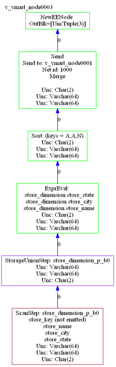
12.1.2 - Query plan cost estimation
The query optimizer chooses a query plan based on cost estimates.
The query optimizer chooses a query plan based on cost estimates. The query optimizer uses information from a number of sources to develop potential plans and determine their relative costs. These include:
-
Number of table rows
-
Column statistics, including: number of distinct values (cardinality), minimum/maximum values, distribution of values, and disk space usage
-
Access path that is likely to require fewest I/O operations, and lowest CPU, memory, and network usage
-
Available eligible projections
-
Join options: join types (merge versus hash joins), join order
-
Query predicates
-
Data segmentation across cluster nodes
Many important optimizer decisions rely on statistics, which the query optimizer uses to determine the final plan to execute a query. Therefore, it is important that statistics be up to date. Without reasonably accurate statistics, the optimizer could choose a suboptimal plan, which might affect query performance.
Vertica provides hints about statistics in the query plan. See Query plan statistics.
Cost versus execution runtime
Although costs correlate to query runtime, they do not provide an estimate of actual runtime. For example, if the optimizer determines that Plan A costs twice as much as Plan B, it is likely that Plan A will require more time to run. However, this cost estimate does not necessarily indicate that Plan A will run twice as long as Plan B.
Also, plan costs for different queries are not directly comparable. For example, if the estimated cost of Plan X for query1 is greater than the cost of Plan Y for query2, it is not necessarily true that Plan X's runtime is greater than Plan Y's runtime.
12.1.3 - Query plan information and structure
Depending on the query and database schema, EXPLAIN output includes the following information:.
Depending on the query and database schema, EXPLAIN output includes the following information:
-
Tables referenced by the statement
-
Estimated costs
-
Estimated row cardinality
-
Path ID, an integer that links to error messages and profiling counters so you troubleshoot performance issues more easily. For more information, see Profiling query plans.
-
Data operations such as SORT, FILTER, LIMIT, and GROUP BY
-
Projections used
-
Information about statistics—for example, whether they are current or out of range
-
Algorithms chosen for operations into the query, such as HASH/MERGE or GROUPBY HASH/GROUPBY PIPELINED
-
Data redistribution (broadcast, segmentation) across cluster nodes
Example
In the EXPLAIN output that follows, the optimizer processes a query in three steps, where each step identified by a unique path ID:
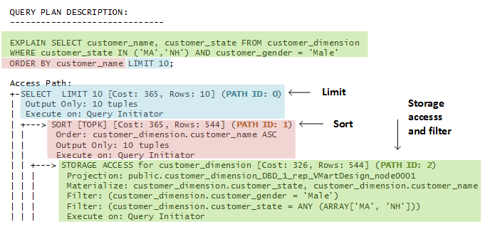
Note
A storage access operation can scan more than the columns in the SELECT list— for example, columns referenced in WHERE clause.
12.1.3.1 - Query plan statistics
If you query a table whose statistics are unavailable or out-of-date, the optimizer might choose a sub-optimal query plan.
If you query a table whose statistics are unavailable or out-of-date, the optimizer might choose a sub-optimal query plan.
You can resolve many issues related to table statistics by calling
ANALYZE_STATISTICS. This function let you update statistics at various scopes: one or more table columns, a single table, or all database tables.
If you update statistics and find that the query still performs sub-optimally, run your query through Database Designer and choose incremental design as the design type.
For detailed information about updating database statistics, see Collecting database statistics.
Statistics hints in query plans
Query plans can contain information about table statistics through two hints: NO STATISTICS and STALE STATISTICS. For example, the following query plan fragment includes NO STATISTICS to indicate that histograms are unavailable:
| | +-- Outer -> STORAGE ACCESS for fact [Cost: 604, Rows: 10K (NO STATISTICS)]
The following query plan fragment includes STALE STATISTICS to indicate that the predicate has fallen outside the histogram range:
| | +-- Outer -> STORAGE ACCESS for fact [Cost: 35, Rows: 1 (STALE STATISTICS)]
12.1.3.2 - Cost and rows path
The following EXPLAIN output shows the Cost operator:.
The following EXPLAIN output shows the Cost operator:
Access Path: +-SELECT LIMIT 10 [Cost: 370, Rows: 10] (PATH ID: 0)
| Output Only: 10 tuples
| Execute on: Query Initiator
| +---> SORT [Cost: 370, Rows: 544] (PATH ID: 1)
| | Order: customer_dimension.customer_name ASC
| | Output Only: 10 tuples
| | Execute on: Query Initiator
| | +---> STORAGE ACCESS for customer_dimension [Cost: 331, Rows: 544] (PATH ID: 2)
| | | Projection: public.customer_dimension_DBD_1_rep_vmartdb_design_vmartdb_design_node0001
| | | Materialize: customer_dimension.customer_state, customer_dimension.customer_name
| | | Filter: (customer_dimension.customer_gender = 'Male')
| | | Filter: (customer_dimension.customer_state = ANY (ARRAY['MA', 'NH']))
| | | Execute on: Query Initiator
The Row operator is the number of rows the optimizer estimates the query will return. Letters after numbers refer to the units of measure (K=thousand, M=million, B=billion, T=trillion), so the output for the following query indicates that the number of rows to return is 50 thousand.
=> EXPLAIN SELECT customer_gender FROM customer_dimension;
Access Path:
+-STORAGE ACCESS for customer_dimension [Cost: 17, Rows: 50K (3 RLE)] (PATH ID: 1)
| Projection: public.customer_dimension_DBD_1_rep_vmartdb_design_vmartdb_design_node0001
| Materialize: customer_dimension.customer_gender
| Execute on: Query Initiator
The reference to (3 RLE) in the STORAGE ACCESS path means that the optimizer estimates that the storage access operator returns 50K rows. Because the column is run-length encoded (RLE), the real number of RLE rows returned is only three rows:
Note
See
Query plans for more information about how the optimizer estimates cost.
12.1.3.3 - Projection path
You can see which the optimizer chose for the query plan by looking at the Projection path in the textual output:.
You can see which projections the optimizer chose for the query plan by looking at the Projection path in the textual output:
EXPLAIN SELECT
customer_name,
customer_state
FROM customer_dimension
WHERE customer_state in ('MA','NH')
AND customer_gender = 'Male'
ORDER BY customer_name
LIMIT 10;
Access Path:
+-SELECT LIMIT 10 [Cost: 370, Rows: 10] (PATH ID: 0)
| Output Only: 10 tuples
| Execute on: Query Initiator
| +---> SORT [Cost: 370, Rows: 544] (PATH ID: 1)
| | Order: customer_dimension.customer_name ASC
| | Output Only: 10 tuples
| | Execute on: Query Initiator
| | +---> STORAGE ACCESS for customer_dimension [Cost: 331, Rows: 544] (PATH ID: 2)
| | | Projection: public.customer_dimension_DBD_1_rep_vmart_vmart_node0001
| | | Materialize: customer_dimension.customer_state, customer_dimension.customer_name
| | | Filter: (customer_dimension.customer_gender = 'Male')
| | | Filter: (customer_dimension.customer_state = ANY (ARRAY['MA', 'NH']))
| | | Execute on: Query Initiator
The query optimizer automatically picks the best projections, but without reasonably accurate statistics, the optimizer could choose a suboptimal projection or join order for a query. For details, see Collecting Statistics.
Vertica considers which projection to choose for a plan by considering the following aspects:
-
How columns are joined in the query
-
How the projections are grouped or sorted
-
Whether SQL analytic operations applied
-
Any column information from a projection's storage on disk
As Vertica scans the possibilities for each plan, projections with the higher initial costs could end up in the final plan because they make joins cheaper. For example, a query can be answered with many possible plans, which the optimizer considers before choosing one of them. For efficiency, the optimizer uses sophisticated algorithms to prune intermediate partial plan fragments with higher cost. The optimizer knows that intermediate plan fragments might initially look bad (due to high storage access cost) but which produce excellent final plans due to other optimizations that it allows.
If your statistics are up to date but the query still performs poorly, run the query through the Database Designer. For details, see Incremental Design.
Tips
-
To test different segmented projections, refer to the projection by name in the query.
-
For optimal performance, write queries so the columns are sorted the same way that the projection columns are sorted.
See also
12.1.3.4 - Join path
Just like a join query, which references two or more tables, the Join step in a query plan has two input branches:.
Just like a join query, which references two or more tables, the Join step in a query plan has two input branches:
-
The left input, which is the outer table of the join
-
The right input, which is the inner table of the join
In the following query, the T1 table is the left input because it is on the left side of the JOIN keyword, and the T2 table is the right input, because it is on the right side of the JOIN keyword:
SELECT * FROM T1 JOIN T2 ON T1.x = T2.x;
Outer versus inner join
Query performance is better if the small table is used as the inner input to the join. The query optimizer automatically reorders the inputs to joins to ensure that this is the case unless the join in question is an outer join.
The following example shows a query and its plan for a left outer join:
=> EXPLAIN SELECT CD.annual_income,OSI.sale_date_key
-> FROM online_sales.online_sales_fact OSI
-> LEFT OUTER JOIN customer_dimension CD ON CD.customer_key = OSI.customer_key;
Access Path:
+-JOIN HASH [LeftOuter] [Cost: 4K, Rows: 5M] (PATH ID: 1)
| Join Cond: (CD.customer_key = OSI.customer_key)
| Materialize at Output: OSI.sale_date_key
| Execute on: All Nodes
| +-- Outer -> STORAGE ACCESS for OSI [Cost: 3K, Rows: 5M] (PATH ID: 2)
| | Projection: online_sales.online_sales_fact_DBD_12_seg_vmartdb_design_vmartdb_design
| | Materialize: OSI.customer_key
| | Execute on: All Nodes
| +-- Inner -> STORAGE ACCESS for CD [Cost: 264, Rows: 50K] (PATH ID: 3)
| | Projection: public.customer_dimension_DBD_1_rep_vmartdb_design_vmartdb_design_node0001
| | Materialize: CD.annual_income, CD.customer_key
| | Execute on: All Nodes
The following example shows a query and its plan for a full outer join:
=> EXPLAIN SELECT CD.annual_income,OSI.sale_date_key
-> FROM online_sales.online_sales_fact OSI
-> FULL OUTER JOIN customer_dimension CD ON CD.customer_key = OSI.customer_key;
Access Path:
+-JOIN HASH [FullOuter] [Cost: 18K, Rows: 5M] (PATH ID: 1) Outer (RESEGMENT) Inner (FILTER)
| Join Cond: (CD.customer_key = OSI.customer_key)
| Execute on: All Nodes
| +-- Outer -> STORAGE ACCESS for OSI [Cost: 3K, Rows: 5M] (PATH ID: 2)
| | Projection: online_sales.online_sales_fact_DBD_12_seg_vmartdb_design_vmartdb_design
| | Materialize: OSI.sale_date_key, OSI.customer_key
| | Execute on: All Nodes
| +-- Inner -> STORAGE ACCESS for CD [Cost: 264, Rows: 50K] (PATH ID: 3)
| | Projection: public.customer_dimension_DBD_1_rep_vmartdb_design_vmartdb_design_node0001
| | Materialize: CD.annual_income, CD.customer_key
| | Execute on: All Nodes
Hash and merge joins
Vertica has two join algorithms to choose from: merge join and hash join. The optimizer automatically chooses the most appropriate algorithm, given the query and projections in a system.
For the following query, the optimizer chooses a hash join.
=> EXPLAIN SELECT CD.annual_income,OSI.sale_date_key
-> FROM online_sales.online_sales_fact OSI
-> INNER JOIN customer_dimension CD ON CD.customer_key = OSI.customer_key;
Access Path:
+-JOIN HASH [Cost: 4K, Rows: 5M] (PATH ID: 1)
| Join Cond: (CD.customer_key = OSI.customer_key)
| Materialize at Output: OSI.sale_date_key
| Execute on: All Nodes
| +-- Outer -> STORAGE ACCESS for OSI [Cost: 3K, Rows: 5M] (PATH ID: 2)
| | Projection: online_sales.online_sales_fact_DBD_12_seg_vmartdb_design_vmartdb_design
| | Materialize: OSI.customer_key
| | Execute on: All Nodes
| +-- Inner -> STORAGE ACCESS for CD [Cost: 264, Rows: 50K] (PATH ID: 3)
| | Projection: public.customer_dimension_DBD_1_rep_vmartdb_design_vmartdb_design_node0001
| | Materialize: CD.annual_income, CD.customer_key
| | Execute on: All Nodes
Tip
If you get a hash join when you are expecting a merge join, it means that at least one of the projections is not sorted on the join column (for example, customer_key in the preceding query). To facilitate a merge join, you might need to create different projections that are sorted on the join columns.
In the next example, the optimizer chooses a merge join. The optimizer's first pass performs a merge join because the inputs are presorted, and then it performs a hash join.
=> EXPLAIN SELECT count(*) FROM online_sales.online_sales_fact OSI
-> INNER JOIN customer_dimension CD ON CD.customer_key = OSI.customer_key
-> INNER JOIN product_dimension PD ON PD.product_key = OSI.product_key;
Access Path:
+-GROUPBY NOTHING [Cost: 8K, Rows: 1] (PATH ID: 1)
| Aggregates: count(*)
| Execute on: All Nodes
| +---> JOIN HASH [Cost: 7K, Rows: 5M] (PATH ID: 2)
| | Join Cond: (PD.product_key = OSI.product_key)
| | Materialize at Input: OSI.product_key
| | Execute on: All Nodes
| | +-- Outer -> JOIN MERGEJOIN(inputs presorted) [Cost: 4K, Rows: 5M] (PATH ID: 3)
| | | Join Cond: (CD.customer_key = OSI.customer_key)
| | | Execute on: All Nodes
| | | +-- Outer -> STORAGE ACCESS for OSI [Cost: 3K, Rows: 5M] (PATH ID: 4)
| | | | Projection: online_sales.online_sales_fact_DBD_12_seg_vmartdb_design_vmartdb_design
| | | | Materialize: OSI.customer_key
| | | | Execute on: All Nodes
| | | +-- Inner -> STORAGE ACCESS for CD [Cost: 132, Rows: 50K] (PATH ID: 5)
| | | | Projection: public.customer_dimension_DBD_1_rep_vmartdb_design_vmartdb_design_node0001
| | | | Materialize: CD.customer_key
| | | | Execute on: All Nodes
| | +-- Inner -> STORAGE ACCESS for PD [Cost: 152, Rows: 60K] (PATH ID: 6)
| | | Projection: public.product_dimension_DBD_2_rep_vmartdb_design_vmartdb_design_node0001
| | | Materialize: PD.product_key
| | | Execute on: All Nodes
Inequality joins
Vertica processes joins with equality predicates very efficiently. The query plan shows equality join predicates as join condition (Join Cond).
=> EXPLAIN SELECT CD.annual_income, OSI.sale_date_key
-> FROM online_sales.online_sales_fact OSI
-> INNER JOIN customer_dimension CD
-> ON CD.customer_key = OSI.customer_key;
Access Path:
+-JOIN HASH [Cost: 4K, Rows: 5M] (PATH ID: 1)
| Join Cond: (CD.customer_key = OSI.customer_key)
| Materialize at Output: OSI.sale_date_key
| Execute on: All Nodes
| +-- Outer -> STORAGE ACCESS for OSI [Cost: 3K, Rows: 5M] (PATH ID: 2)
| | Projection: online_sales.online_sales_fact_DBD_12_seg_vmartdb_design_vmartdb_design
| | Materialize: OSI.customer_key
| | Execute on: All Nodes
| +-- Inner -> STORAGE ACCESS for CD [Cost: 264, Rows: 50K] (PATH ID: 3)
| | Projection: public.customer_dimension_DBD_1_rep_vmartdb_design_vmartdb_design_node0001
| | Materialize: CD.annual_income, CD.customer_key
| | Execute on: All Nodes
However, inequality joins are treated like cross joins and can run less efficiently, which you can see by the change in cost between the two queries:
=> EXPLAIN SELECT CD.annual_income, OSI.sale_date_key
-> FROM online_sales.online_sales_fact OSI
-> INNER JOIN customer_dimension CD
-> ON CD.customer_key < OSI.customer_key;
Access Path:
+-JOIN HASH [Cost: 98M, Rows: 5M] (PATH ID: 1)
| Join Filter: (CD.customer_key < OSI.customer_key)
| Materialize at Output: CD.annual_income
| Execute on: All Nodes
| +-- Outer -> STORAGE ACCESS for CD [Cost: 132, Rows: 50K] (PATH ID: 2)
| | Projection: public.customer_dimension_DBD_1_rep_vmartdb_design_vmartdb_design_node0001
| | Materialize: CD.customer_key
| | Execute on: All Nodes
| +-- Inner -> STORAGE ACCESS for OSI [Cost: 3K, Rows: 5M] (PATH ID: 3)
| | Projection: online_sales.online_sales_fact_DBD_12_seg_vmartdb_design_vmartdb_design
| | Materialize: OSI.sale_date_key, OSI.customer_key
| | Execute on: All Nodes
Event series joins
Event series joins are denoted by the INTERPOLATED path.
=> EXPLAIN SELECT * FROM hTicks h FULL OUTER JOIN aTicks a -> ON (h.time INTERPOLATE PREVIOUS
Access Path:
+-JOIN (INTERPOLATED) [FullOuter] [Cost: 31, Rows: 4 (NO STATISTICS)] (PATH ID: 1)
Outer (SORT ON JOIN KEY) Inner (SORT ON JOIN KEY)
| Join Cond: (h."time" = a."time")
| Execute on: Query Initiator
| +-- Outer -> STORAGE ACCESS for h [Cost: 15, Rows: 4 (NO STATISTICS)] (PATH ID: 2)
| | Projection: public.hTicks_node0004
| | Materialize: h.stock, h."time", h.price
| | Execute on: Query Initiator
| +-- Inner -> STORAGE ACCESS for a [Cost: 15, Rows: 4 (NO STATISTICS)] (PATH ID: 3)
| | Projection: public.aTicks_node0004
| | Materialize: a.stock, a."time", a.price
| | Execute on: Query Initiator
12.1.3.5 - Path ID
The PATH ID is a unique identifier that Vertica assigns to each operation (path) within a query plan.
The PATH ID is a unique identifier that Vertica assigns to each operation (path) within a query plan. The same identifier is shared by:
Path IDs can help you trace issues to their root cause. For example, if a query returns a join error, preface the query with EXPLAIN and look for PATH ID n in the query plan to see which join in the query had the problem.
For example, the following EXPLAIN output shows the path ID for each path in the optimizer's query plan:
=> EXPLAIN SELECT * FROM fact JOIN dim ON x=y JOIN ext on y=z;
Access Path:
+-JOIN MERGEJOIN(inputs presorted) [Cost: 815, Rows: 10K (NO STATISTICS)] (PATH ID: 1)
| Join Cond: (dim.y = ext.z)
| Materialize at Output: fact.x
| Execute on: All Nodes
| +-- Outer -> JOIN MERGEJOIN(inputs presorted) [Cost: 408, Rows: 10K (NO STATISTICS)] (PATH ID: 2)
| | Join Cond: (fact.x = dim.y)
| | Execute on: All Nodes
| | +-- Outer -> STORAGE ACCESS for fact [Cost: 202, Rows: 10K (NO STATISTICS)] (PATH ID: 3)
| | | Projection: public.fact_super
| | | Materialize: fact.x
| | | Execute on: All Nodes
| | +-- Inner -> STORAGE ACCESS for dim [Cost: 202, Rows: 10K (NO STATISTICS)] (PATH ID: 4)
| | | Projection: public.dim_super
| | | Materialize: dim.y
| | | Execute on: All Nodes
| +-- Inner -> STORAGE ACCESS for ext [Cost: 202, Rows: 10K (NO STATISTICS)] (PATH ID: 5)
| | Projection: public.ext_super
| | Materialize: ext.z
| | Execute on: All Nodes
12.1.3.6 - Filter path
The Filter step evaluates predicates on a single table.
The Filter step evaluates predicates on a single table. It accepts a set of rows, eliminates some of them (based on the criteria you provide in your query), and returns the rest. For example, the optimizer can filter local data of a join input that will be joined with another re-segmented join input.
The following statement queries the customer_dimension table and uses the WHERE clause to filter the results only for male customers in Massachusetts and New Hampshire.
EXPLAIN SELECT
CD.customer_name,
CD.customer_state,
AVG(CD.customer_age) AS avg_age,
COUNT(*) AS count
FROM customer_dimension CD
WHERE CD.customer_state in ('MA','NH') AND CD.customer_gender = 'Male'
GROUP BY CD.customer_state, CD.customer_name;
The query plan output is as follows:
Access Path:
+-GROUPBY HASH [Cost: 378, Rows: 544] (PATH ID: 1)
| Aggregates: sum_float(CD.customer_age), count(CD.customer_age), count(*)
| Group By: CD.customer_state, CD.customer_name
| Execute on: Query Initiator
| +---> STORAGE ACCESS for CD [Cost: 372, Rows: 544] (PATH ID: 2)
| | Projection: public.customer_dimension_DBD_1_rep_vmartdb_design_vmartdb_design_node0001
| | Materialize: CD.customer_state, CD.customer_name, CD.customer_age
| | Filter: (CD.customer_gender = 'Male')
| | Filter: (CD.customer_state = ANY (ARRAY['MA', 'NH']))
| | Execute on: Query Initiator
12.1.3.7 - GROUP BY paths
A GROUP BY operation has two algorithms:.
A GROUP BY operation has two algorithms:
-
GROUPBY HASH input is not sorted by the group columns, so Vertica builds a hash table on those group columns in order to process the aggregates and group by expressions.
-
GROUPBY PIPELINED requires that inputs be presorted on the columns specified in the group, which means that Vertica need only retain data in the current group in memory. GROUPBY PIPELINED operations are preferred because they are generally faster and require less memory than GROUPBY HASH. GROUPBY PIPELINED is especially useful for queries that process large numbers of high-cardinality group by columns or DISTINCT aggregates.
If possible, the query optimizer chooses the faster algorithm GROUPBY PIPELINED over GROUPBY HASH.
12.1.3.7.1 - GROUPBY HASH query plan
Here's an example of how GROUPBY HASH operations look in EXPLAIN output.
Here's an example of how GROUPBY HASH operations look in EXPLAIN output.
=> EXPLAIN SELECT COUNT(DISTINCT annual_income)
FROM customer_dimension
WHERE customer_region='NorthWest';
The output shows that the optimizer chose the less efficient GROUPBY HASH path, which means the projection was not presorted on the annual_income column. If such a projection is available, the optimizer would choose the GROUPBY PIPELINED algorithm.
Access Path:
+-GROUPBY NOTHING [Cost: 256, Rows: 1 (NO STATISTICS)] (PATH ID: 1)
| Aggregates: count(DISTINCT customer_dimension.annual_income)
| +---> GROUPBY HASH (LOCAL RESEGMENT GROUPS) [Cost: 253, Rows: 10K (NO STATISTICS)] (PATH ID: 2)
| | Group By: customer_dimension.annual_income
| | +---> STORAGE ACCESS for customer_dimension [Cost: 227, Rows: 50K (NO STATISTICS)] (PATH ID: 3)
| | | Projection: public.customer_dimension_super
| | | Materialize: customer_dimension.annual_income
| | | Filter: (customer_dimension.customer_region = 'NorthWest'
...
12.1.3.7.2 - GROUPBY PIPELINED query plan
If you have a projection that is already sorted on the customer_gender column, the optimizer chooses the faster GROUPBY PIPELINED operation:.
If you have a projection that is already sorted on the customer_gender column, the optimizer chooses the faster GROUPBY PIPELINED operation:
=> EXPLAIN SELECT COUNT(distinct customer_gender) from customer_dimension;
Access Path:
+-GROUPBY NOTHING [Cost: 22, Rows: 1] (PATH ID: 1)
| Aggregates: count(DISTINCT customer_dimension.customer_gender)
| Execute on: Query Initiator
| +---> GROUPBY PIPELINED [Cost: 20, Rows: 10K] (PATH ID: 2)
| | Group By: customer_dimension.customer_gender
| | Execute on: Query Initiator
| | +---> STORAGE ACCESS for customer_dimension [Cost: 17, Rows: 50K (3 RLE)] (PATH ID: 3)
| | | Projection: public.customer_dimension_DBD_1_rep_vmartdb_design_vmartdb_design_node0001
| | | Materialize: customer_dimension.customer_gender
| | | Execute on: Query Initiator
Similarly, the use of an equality predicate, such as in the following query, preserves GROUPBY PIPELINED:
=> EXPLAIN SELECT COUNT(DISTINCT annual_income) FROM customer_dimension
WHERE customer_gender = 'Female';
Access Path: +-GROUPBY NOTHING [Cost: 161, Rows: 1] (PATH ID: 1)
| Aggregates: count(DISTINCT customer_dimension.annual_income)
| +---> GROUPBY PIPELINED [Cost: 158, Rows: 10K] (PATH ID: 2)
| | Group By: customer_dimension.annual_income
| | +---> STORAGE ACCESS for customer_dimension [Cost: 144, Rows: 47K] (PATH ID: 3)
| | | Projection: public.customer_dimension_DBD_1_rep_vmartdb_design_vmartdb_design_node0001
| | | Materialize: customer_dimension.annual_income
| | | Filter: (customer_dimension.customer_gender = 'Female')
Tip
If EXPLAIN reports GROUPBY HASH, modify the projection design to force it to use GROUPBY PIPELINED.
12.1.3.8 - Sort path
The SORT operator sorts the data according to a specified list of columns.
The SORT operator sorts the data according to a specified list of columns. The EXPLAIN output indicates the sort expressions and if the sort order is ascending (ASC) or descending (DESC).
For example, the following query plan shows the column list nature of the SORT operator:
EXPLAIN SELECT
CD.customer_name,
CD.customer_state,
AVG(CD.customer_age) AS avg_age,
COUNT(*) AS count
FROM customer_dimension CD
WHERE CD.customer_state in ('MA','NH')
AND CD.customer_gender = 'Male'
GROUP BY CD.customer_state, CD.customer_name
ORDER BY avg_age, customer_name;
Access Path:
+-SORT [Cost: 422, Rows: 544] (PATH ID: 1)
| Order: (<SVAR> / float8(<SVAR>)) ASC, CD.customer_name ASC
| Execute on: Query Initiator
| +---> GROUPBY HASH [Cost: 378, Rows: 544] (PATH ID: 2)
| | Aggregates: sum_float(CD.customer_age), count(CD.customer_age), count(*)
| | Group By: CD.customer_state, CD.customer_name
| | Execute on: Query Initiator
| | +---> STORAGE ACCESS for CD [Cost: 372, Rows: 544] (PATH ID: 3)
| | | Projection: public.customer_dimension_DBD_1_rep_vmart_vmart_node0001
| | | Materialize: CD.customer_state, CD.customer_name, CD.customer_age
| | | Filter: (CD.customer_gender = 'Male')
| | | Filter: (CD.customer_state = ANY (ARRAY['MA', 'NH']))
| | | Execute on: Query Initiator
If you change the sort order to descending, the change appears in the query plan:
EXPLAIN SELECT
CD.customer_name,
CD.customer_state,
AVG(CD.customer_age) AS avg_age,
COUNT(*) AS count
FROM customer_dimension CD
WHERE CD.customer_state in ('MA','NH')
AND CD.customer_gender = 'Male'
GROUP BY CD.customer_state, CD.customer_name
ORDER BY avg_age DESC, customer_name;
Access Path:
+-SORT [Cost: 422, Rows: 544] (PATH ID: 1)
| Order: (<SVAR> / float8(<SVAR>)) DESC, CD.customer_name ASC
| Execute on: Query Initiator
| +---> GROUPBY HASH [Cost: 378, Rows: 544] (PATH ID: 2)
| | Aggregates: sum_float(CD.customer_age), count(CD.customer_age), count(*)
| | Group By: CD.customer_state, CD.customer_name
| | Execute on: Query Initiator
| | +---> STORAGE ACCESS for CD [Cost: 372, Rows: 544] (PATH ID: 3)
| | | Projection: public.customer_dimension_DBD_1_rep_vmart_vmart_node0001
| | | Materialize: CD.customer_state, CD.customer_name, CD.customer_age
| | | Filter: (CD.customer_gender = 'Male')
| | | Filter: (CD.customer_state = ANY (ARRAY['MA', 'NH']))
| | | Execute on: Query Initiator
12.1.3.9 - Limit path
The LIMIT path restricts the number of result rows based on the LIMIT clause in the query.
The LIMIT path restricts the number of result rows based on the LIMIT clause in the query. Using the LIMIT clause in queries with thousands of rows might increase query performance.
The optimizer pushes the LIMIT operation as far down as possible in queries. A single LIMIT clause in the query can generate multiple Output Only plan annotations.
=> EXPLAIN SELECT COUNT(DISTINCT annual_income) FROM customer_dimension LIMIT 10;
Access Path:
+-SELECT LIMIT 10 [Cost: 161, Rows: 10] (PATH ID: 0)
| Output Only: 10 tuples
| +---> GROUPBY NOTHING [Cost: 161, Rows: 1] (PATH ID: 1)
| | Aggregates: count(DISTINCT customer_dimension.annual_income)
| | Output Only: 10 tuples
| | +---> GROUPBY HASH (SORT OUTPUT) [Cost: 158, Rows: 10K] (PATH ID: 2)
| | | Group By: customer_dimension.annual_income
| | | +---> STORAGE ACCESS for customer_dimension [Cost: 132, Rows: 50K] (PATH ID: 3)
| | | | Projection: public.customer_dimension_DBD_1_rep_vmartdb_design_vmartdb_design_node0001
| | | | Materialize: customer_dimension.annual_income
12.1.3.10 - Data redistribution path
The optimizer can redistribute join data in two ways:.
The optimizer can redistribute join data in two ways:
-
Broadcasting
-
Resegmentation
Broadcasting
Broadcasting sends a complete copy of an intermediate result to all nodes in the cluster. Broadcast is used for joins in the following cases:
-
One table is very small (usually the inner table) compared to the other.
-
Vertica can avoid other large upstream resegmentation operations.
-
Outer join or subquery semantics require one side of the join to be replicated.
For example:
=> EXPLAIN SELECT * FROM T1 LEFT JOIN T2 ON T1.a > T2.y;
Access Path:
+-JOIN HASH [LeftOuter] [Cost: 40K, Rows: 10K (NO STATISTICS)] (PATH ID: 1) Inner (BROADCAST)
| Join Filter: (T1.a > T2.y)
| Materialize at Output: T1.b
| Execute on: All Nodes
| +-- Outer -> STORAGE ACCESS for T1 [Cost: 151, Rows: 10K (NO STATISTICS)] (PATH ID: 2)
| | Projection: public.T1_b0
| | Materialize: T1.a
| | Execute on: All Nodes
| +-- Inner -> STORAGE ACCESS for T2 [Cost: 302, Rows: 10K (NO STATISTICS)] (PATH ID: 3)
| | Projection: public.T2_b0
| | Materialize: T2.x, T2.y
| | Execute on: All Nodes
Resegmentation
Resegmentation takes an existing projection or intermediate relation and resegments the data evenly across all cluster nodes. At the end of the resegmentation operation, every row from the input relation is on exactly one node. Resegmentation is the operation used most often for distributed joins in Vertica if the data is not already segmented for local joins. For more detail, see Identical segmentation.
For example:
=> CREATE TABLE T1 (a INT, b INT) SEGMENTED BY HASH(a) ALL NODES;
=> CREATE TABLE T2 (x INT, y INT) SEGMENTED BY HASH(x) ALL NODES;
=> EXPLAIN SELECT * FROM T1 JOIN T2 ON T1.a = T2.y;
------------------------------ QUERY PLAN DESCRIPTION: ------------------------------
Access Path:
+-JOIN HASH [Cost: 639, Rows: 10K (NO STATISTICS)] (PATH ID: 1) Inner (RESEGMENT)
| Join Cond: (T1.a = T2.y)
| Materialize at Output: T1.b
| Execute on: All Nodes
| +-- Outer -> STORAGE ACCESS for T1 [Cost: 151, Rows: 10K (NO STATISTICS)] (PATH ID: 2)
| | Projection: public.T1_b0
| | Materialize: T1.a
| | Execute on: All Nodes
| +-- Inner -> STORAGE ACCESS for T2 [Cost: 302, Rows: 10K (NO STATISTICS)] (PATH ID: 3)
| | Projection: public.T2_b0
| | Materialize: T2.x, T2.y
| | Execute on: All Nodes
12.1.3.11 - Analytic function path
Vertica attempts to optimize multiple SQL-99 Analytic Functions from the same query by grouping them together in Analytic Group areas.
Vertica attempts to optimize multiple SQL-99 Analytic functions from the same query by grouping them together in Analytic Group areas.
For each analytical group, Vertica performs a distributed sort and resegment of the data, if necessary.
You can tell how many sorts and resegments are required based on the query plan.
For example, the following query plan shows that the
FIRST_VALUE and
LAST_VALUE functions are in the same analytic group because their OVER clause is the same. In contrast, ROW_NUMBER() has a different ORDER BY clause, so it is in a different analytic group. Because both groups share the same PARTITION BY deal_stage clause, the data does not need to be resegmented between groups :
EXPLAIN SELECT
first_value(deal_size) OVER (PARTITION BY deal_stage
ORDER BY deal_size),
last_value(deal_size) OVER (PARTITION BY deal_stage
ORDER BY deal_size),
row_number() OVER (PARTITION BY deal_stage
ORDER BY largest_bill_amount)
FROM customer_dimension;
Access Path:
+-ANALYTICAL [Cost: 1K, Rows: 50K] (PATH ID: 1)
| Analytic Group
| Functions: row_number()
| Group Sort: customer_dimension.deal_stage ASC, customer_dimension.largest_bill_amount ASC NULLS LAST
| Analytic Group
| Functions: first_value(), last_value()
| Group Filter: customer_dimension.deal_stage
| Group Sort: customer_dimension.deal_stage ASC, customer_dimension.deal_size ASC NULL LAST
| Execute on: All Nodes
| +---> STORAGE ACCESS for customer_dimension [Cost: 263, Rows: 50K]
(PATH ID: 2)
| | Projection: public.customer_dimension_DBD_1_rep_vmart_vmart_node0001
| | Materialize: customer_dimension.largest_bill_amount,
customer_dimension.deal_stage, customer_dimension.deal_size
| | Execute on: All Nodes
See also
Invoking analytic functions
12.1.3.12 - Node down information
Vertica provides performance optimization when cluster nodes fail by distributing the work of the down nodes uniformly among available nodes throughout the cluster.
Vertica provides performance optimization when cluster nodes fail by distributing the work of the down nodes uniformly among available nodes throughout the cluster.
When a node in your cluster is down, the query plan identifies which node the query will execute on. To help you quickly identify down nodes on large clusters, EXPLAIN output lists up to six nodes, if the number of running nodes is less than or equal to six, and lists only down nodes if the number of running nodes is more than six.
Note
The node that executes down node queries is not always the same one.
The following table provides more detail:
|
Node state |
EXPLAIN output |
If all nodes are up, EXPLAIN output indicates All Nodes. |
Execute on: All Nodes |
If fewer than 6 nodes are up, EXPLAIN lists up to six running nodes. |
Execute on: [node_list]. |
If more than 6 nodes are up, EXPLAIN lists only non-running nodes. |
Execute on: All Nodes Except [node_list] |
If the node list contains non-ephemeral nodes, the EXPLAIN output indicates All Permanent Nodes. |
Execute on: All Permanent Nodes |
If the path is being run on the query initiator, the EXPLAIN output indicates Query Initiator. |
Execute on: Query Initiator |
Examples
In the following example, the down node is v_vmart_node0005, and the node v_vmart_node0006 will execute this run of the query.
=> EXPLAIN SELECT * FROM test;
QUERY PLAN
-----------------------------------------------------------------------------
QUERY PLAN DESCRIPTION:
------------------------------
EXPLAIN SELECT * FROM my1table;
Access Path:
+-STORAGE ACCESS for my1table [Cost: 10, Rows: 2] (PATH ID: 1)
| Projection: public.my1table_b0
| Materialize: my1table.c1, my1table.c2
| Execute on: All Except v_vmart_node0005
+-STORAGE ACCESS for my1table (REPLACEMENT FOR DOWN NODE) [Cost: 66, Rows: 2]
| Projection: public.my1table_b1
| Materialize: my1table.c1, my1table.c2
| Execute on: v_vmart_node0006
The All Permanent Nodes output in the following example fragment denotes that the node list is for permanent (non-ephemeral) nodes only:
=> EXPLAIN SELECT * FROM my2table;
Access Path:
+-STORAGE ACCESS for my2table [Cost: 18, Rows:6 (NO STATISTICS)] (PATH ID: 1)
| Projection: public.my2tablee_b0
| Materialize: my2table.x, my2table.y, my2table.z
| Execute on: All Permanent Nodes
12.1.3.13 - MERGE path
Vertica prepares an optimized query plan for a MERGE statement if the statement and its tables meet the criteria described in Improving MERGE Performance.
Vertica prepares an optimized query plan for a
MERGE statement if the statement and its tables meet the criteria described in MERGE optimization.
Use the
EXPLAIN keyword to determine whether Vertica can produce an optimized query plan for a given MERGE statement. If optimization is possible, the EXPLAIN-generated output contains a[Semi] path, as shown in the following sample fragment:
...
Access Path:
+-DML DELETE [Cost: 0, Rows: 0]
| Target Projection: public.A_b1 (DELETE ON CONTAINER)
| Target Prep:
| Execute on: All Nodes
| +---> JOIN MERGEJOIN(inputs presorted) [Semi] [Cost: 6, Rows: 1 (NO STATISTICS)] (PATH ID: 1)
Inner (RESEGMENT)
| | Join Cond: (A.a1 = VAL(2))
| | Execute on: All Nodes
| | +-- Outer -> STORAGE ACCESS for A [Cost: 2, Rows: 2 (NO STATISTICS)] (PATH ID: 2)
...
Conversely, if Vertica cannot create an optimized plan, EXPLAIN-generated output contains RightOuter path:
...
Access Path: +-DML MERGE
| Target Projection: public.locations_b1
| Target Projection: public.locations_b0
| Target Prep:
| Execute on: All Nodes
| +---> JOIN MERGEJOIN(inputs presorted) [RightOuter] [Cost: 28, Rows: 3 (NO STATISTICS)] (PATH ID: 1) Outer (RESEGMENT) Inner (RESEGMENT)
| | Join Cond: (locations.user_id = VAL(2)) AND (locations.location_x = VAL(2)) AND (locations.location_y = VAL(2))
| | Execute on: All Nodes
| | +-- Outer -> STORAGE ACCESS for <No Alias> [Cost: 15, Rows: 2 (NO STATISTICS)] (PATH ID: 2)
...
12.2 - Directed queries
Directed queries encapsulate information that the optimizer can use to create a query plan.
Directed queries encapsulate information that the optimizer can use to create a query plan. Directed queries can serve the following goals:
-
Preserve current query plans before a scheduled upgrade. In most instances, queries perform more efficiently after a Vertica upgrade. In the few cases where this is not so, you can use directed queries that you created before upgrading, to recreate query plans from the earlier version.
-
Enable you to create query plans that improve optimizer performance. Occasionally, you might want to influence the optimizer to make better choices in executing a given query. For example, you can choose a different projection, or force a different join order. In this case, you can use a directed query to create a query plan that preempts any plan that the optimizer might otherwise create.
-
Redirect an input query to a query that uses different semantics—for example, map a join query to a SELECT statement that queries a flattened table.
Directed query components
A directed query pairs two components:
-
Input query: A query that triggers use of this directed query when it is active.
-
Annotated query: A SQL statement with embedded optimizer hints, which instruct the optimizer how to create a query plan for the specified input query. These hints specify important query plan elements, such as join order and projection choices.
Tip
You can also use most optimizer hints directly in vsql. For details, see
Hints.
Vertica provides two methods for creating directed queries:
For a description of both methods, see Creating directed queries.
12.2.1 - Creating directed queries
CREATE DIRECTED QUERY associates an input query with a query annotated with optimizer hints.
CREATE DIRECTED QUERY associates an input query with a query annotated with optimizer hints. It stores the association under a unique identifier.
CREATE DIRECTED QUERY has two variants:
- CREATE DIRECTED QUERY OPTIMIZER directs the query optimizer to generate annotated SQL from the specified input query. The annotated query contains hints that the optimizer can use to recreate its current query plan for that input query.
- CREATE DIRECTED QUERY CUSTOM specifies an annotated query supplied by the user. Vertica associates the annotated query with the input query specified by the last SAVE QUERY statement.
In both cases, Vertica associates the annotated query and input query, and registers their association in the system table DIRECTED_QUERIES under query_name.
The two approaches can be used together: you can use the annotated SQL that the optimizer creates as the basis for creating your own (custom) directed queries.
12.2.1.1 - Optimizer-generated directed queries
CREATE DIRECTED QUERY OPTIMIZER passes an input query to the optimizer, which generates an annotated query from its own query plan.
CREATE DIRECTED QUERY OPTIMIZER passes an input query to the optimizer, which generates an annotated query from its own query plan. It then pairs the input and annotated queries and saves them as a directed query. This directed query can be used to handle other queries that are identical except for the predicate strings on which query results are filtered.
You can use optimizer-generated directed queries to capture query plans before you upgrade. Doing so can be especially useful if you detect diminished performance of a given query after the upgrade. In this case, you can use the corresponding directed query to recreate an earlier query plan, and compare its performance to the plan generated by the current optimizer.
You can also create multiple optimizer-generated directed queries from the most frequently executed queries, by invoking the meta-function SAVE_PLANS. For details, see Bulk-Creation of Directed Queries.
Example
The following SQL statements create and activate the directed query findEmployeesCityJobTitle_OPT:
=> CREATE DIRECTED QUERY OPTIMIZER 'findEmployeesCityJobTitle_OPT'
SELECT employee_first_name, employee_last_name FROM public.employee_dimension
WHERE employee_city='Boston' and job_title='Cashier' ORDER BY employee_last_name, employee_first_name;
CREATE DIRECTED QUERY
=> ACTIVATE DIRECTED QUERY findEmployeesCityJobTitle_OPT;
ACTIVATE DIRECTED QUERY
After this directed query plan is activated, the optimizer uses it to generate a query plan for all subsequent invocations of this input query, and others like it. You can view the optimizer-generated annotated query by calling GET DIRECTED QUERY or querying system table DIRECTED_QUERIES:
=> SELECT input_query, annotated_query FROM V_CATALOG.DIRECTED_QUERIES
WHERE query_name = 'findEmployeesCityJobTitle_OPT';
-[ RECORD 1 ]---+----------------------------------------------------------------------------
input_query | SELECT employee_dimension.employee_first_name, employee_dimension.employee_last_name FROM public.employee_dimension
WHERE ((employee_dimension.employee_city = 'Boston'::varchar(6) /*+:v(1)*/) AND (employee_dimension.job_title = 'Cashier'::varchar(7) /*+:v(2)*/))
ORDER BY employee_dimension.employee_last_name, employee_dimension.employee_first_name
annotated_query | SELECT /*+verbatim*/ employee_dimension.employee_first_name AS employee_first_name, employee_dimension.employee_last_name AS employee_last_name FROM public.employee_dimension AS employee_dimension/*+projs('public.employee_dimension')*/
WHERE (employee_dimension.employee_city = 'Boston'::varchar(6) /*+:v(1)*/) AND (employee_dimension.job_title = 'Cashier'::varchar(7) /*+:v(2)*/)
ORDER BY 2 ASC, 1 ASC
In this case, the annotated query includes the following hints:
-
/*+verbatim*/ specifies to execute the annotated query exactly as written and produce a query plan accordingly.
-
/*+projs('public.Emp_Dimension')*/ directs the optimizer to create a query plan that uses the projection public.Emp_Dimension.
/*+:v(n)*/ (alias of /*+IGNORECONST(n)*/) is included several times in the annotated and input queries. These hints qualify two constants in the query predicates: Boston and Cashier. Each :v hint has an integer argument n that pairs corresponding constants in the input and annotated query queries: *+:v(1)*/ for Boston, and /*+:v(2)*/ for Cashier. The hints tell the optimizer to disregard these constants when it decides whether to apply this directed query to other input queries that are similar. Thus, ignore constant hints can let you use the same directed query for different input queries.
The following query uses different values for the columns employee_city and job_title, but is otherwise identical to the original input query of directed query EmployeesCityJobTitle_OPT:
=> SELECT employee_first_name, employee_last_name FROM public.employee_dimension
WHERE employee_city = 'San Francisco' and job_title = 'Branch Manager' ORDER BY employee_last_name, employee_first_name;
If the directed query EmployeesCityJobTitle_OPT is active, the optimizer can use it for this query:
=> EXPLAIN SELECT employee_first_name, employee_last_name FROM employee_dimension
WHERE employee_city='San Francisco' AND job_title='Branch Manager' ORDER BY employee_last_name, employee_first_name;
...
------------------------------
QUERY PLAN DESCRIPTION:
------------------------------
EXPLAIN SELECT employee_first_name, employee_last_name FROM employee_dimension WHERE employee_city='San Francisco' AND job_title='Branch Manager' ORDER BY employee_last_name, employee_first_name;
The following active directed query(query name: findEmployeesCityJobTitle_OPT) is being executed:
SELECT /*+verbatim*/ employee_dimension.employee_first_name, employee_dimension.employee_last_name
FROM public.employee_dimension employee_dimension/*+projs('public.employee_dimension')*/
WHERE ((employee_dimension.employee_city = 'San Francisco'::varchar(13)) AND (employee_dimension.job_title = 'Branch Manager'::varchar(14)))
ORDER BY employee_dimension.employee_last_name, employee_dimension.employee_first_name
Access Path:
+-SORT [Cost: 222, Rows: 10K (NO STATISTICS)] (PATH ID: 1)
| Order: employee_dimension.employee_last_name ASC, employee_dimension.employee_first_name ASC
| Execute on: All Nodes
| +---> STORAGE ACCESS for employee_dimension [Cost: 60, Rows: 10K (NO STATISTICS)] (PATH ID: 2)
| | Projection: public.employee_dimension_super
| | Materialize: employee_dimension.employee_first_name, employee_dimension.employee_last_name
| | Filter: (employee_dimension.employee_city = 'San Francisco')
| | Filter: (employee_dimension.job_title = 'Branch Manager')
| | Execute on: All Nodes
...
Bulk-creation of directed queries
The meta-function SAVE_PLANS lets you create multiple optimizer-generated directed queries from the most frequently executed queries. SAVE_PLANS works as follows:
-
Iterates over all queries in the data collector table dc_requests_issued and selects the most-frequently requested queries, up to the maximum specified by its query‑budget argument. If the meta-function's since‑date argument is also set, then SAVE_PLANS iterates only over queries that were issued on or after the specified date.
As SAVE_PLANS iterates over dc_requests_issued, it tests queries against various restrictions. In general, directed queries support only SELECT statements as input. Within this broad requirement, input queries are subject to other restrictions.
-
Calls CREATE DIRECTED QUERY OPTIMIZER on all qualifying input queries, which creates a directed query for each unique input query as described above.
-
Saves metadata on the new set of directed queries to system table DIRECTED_QUERIES, where all directed queries of that set share the same SAVE_PLANS_VERSION integer. This integer is computed from the highest SAVE_PLANS_VERSION + 1.
You can later use SAVE_PLANS_VERSION identifiers to bulk activate, deactivate, and drop directed queries. For example:
=> SELECT save_plans (40);
save_plans
-------------------------------------------------------------------------------------------------------------
9 directed query supported queries out of 40 most frequently run queries were saved under the save_plans_version 3.
To view the saved queries, run:
SELECT * FROM directed_queries WHERE save_plans_version = '3';
To drop the saved queries, run:
DROP DIRECTED QUERY WHERE save_plans_version = '3';
(1 row)
=> SELECT input_query::VARCHAR(60) FROM directed_queries WHERE save_plans_version = 3 AND input_query ILIKE '%line_search%';
input_query
--------------------------------------------------------------
SELECT public.line_search_logistic2(udtf1.deviance, udtf1.G
SELECT public.line_search_logistic2(udtf1.deviance, udtf1.G
(2 rows)
=> ACTIVATE DIRECTED QUERY WHERE save_plans_version = 3 AND input_query ILIKE '%line_search%';
ACTIVATE DIRECTED QUERY
=> SELECT query_name, input_query::VARCHAR(60), is_active FROM directed_queries WHERE save_plans_version = 3 AND input_query ILIKE '%line_search%';
query_name | input_query | is_active
------------------------+--------------------------------------------------------------+-----------
save_plans_nolabel_3_3 | SELECT public.line_search_logistic2(udtf1.deviance, udtf1.G | t
save_plans_nolabel_6_3 | SELECT public.line_search_logistic2(udtf1.deviance, udtf1.G | t
(2 rows)
Note
query_name values are concatenated from the following strings:
save_plans_query‑label_query‑number_save‑plans‑version
where:
query-label is a LABEL hint embedded in the input query associated with this directed query. If theinput query contains no label, then this string is set to nolabel.query‑number is an integer in a continuous sequence between 0 and budget-query, which uniquely identifies this directed query from others in the same SAVE_PLANS-generated set.- [save‑plans‑version](/en/sql-reference/system-tables/v-catalog-schema/directed-queries/#SAVE_PLANS_VERSION) identifies the set of directed queries to which this directed query belongs.
12.2.1.2 - Custom directed queries
CREATE DIRECTED QUERY CUSTOM specifies an annotated query and pairs it to an input query previously saved by SAVE QUERY.
CREATE DIRECTED QUERY CUSTOM specifies an annotated query and pairs it to an input query previously saved by SAVE QUERY. You must issue both statements in the same user session.
For example, you might want a query to use a specific projection:
-
Specify the query with SAVE QUERY:
=> SAVE QUERY SELECT employee_first_name, employee_last_name FROM employee_dimension
WHERE employee_city='Boston' AND job_title='Cashier';
SAVE QUERY
Note
The input query that you supply to SAVE QUERY only supports the
:v hint.
-
Create a custom directed query with CREATE DIRECTED QUERY CUSTOM, which specifies an annotated query and associates it with the saved query. The annotated query includes a /*+projs*/ hint, which instructs the optimizer to use the projection public.emp_dimension_unseg when users call the saved query:
=> CREATE DIRECTED QUERY CUSTOM 'findBostonCashiers_CUSTOM'
SELECT employee_first_name, employee_last_name
FROM employee_dimension /*+Projs('public.emp_dimension_unseg')*/
WHERE employee_city='Boston' AND job_title='Cashier';
CREATE DIRECTED QUERY
Caution
Vertica associates a saved query and annotated query without checking whether the input and annotated queries are compatible. Be careful to sequence SAVE QUERY and CREATE DIRECTED QUERY CUSTOM statements so the saved and directed queries are correctly matched.
-
Activate the directed query:
=> ACTIVATE DIRECTED QUERY findBostonCashiers_CUSTOM;
ACTIVATE DIRECTED QUERY
-
After activation, the optimizer uses this directed query to generate a query plan for all subsequent invocations of its input query. The following EXPLAIN output verifies the optimizer's use of this directed query and the projection it specifies:
=> EXPLAIN SELECT employee_first_name, employee_last_name FROM employee_dimension
WHERE employee_city='Boston' AND job_title='Cashier';
QUERY PLAN
------------------------------
QUERY PLAN DESCRIPTION:
------------------------------
EXPLAIN SELECT employee_first_name, employee_last_name FROM employee_dimension where employee_city='Boston' AND job_title='Cashier';
The following active directed query(query name: findBostonCashiers_CUSTOM) is being executed:
SELECT employee_dimension.employee_first_name, employee_dimension.employee_last_name
FROM public.employee_dimension/*+Projs('public.emp_dimension_unseg')*/
WHERE ((employee_dimension.employee_city = 'Boston'::varchar(6)) AND (employee_dimension.job_title = 'Cashier'::varchar(7)))
Access Path:
+-STORAGE ACCESS for employee_dimension [Cost: 158, Rows: 10K (NO STATISTICS)] (PATH ID: 1)
| Projection: public.emp_dimension_unseg
| Materialize: employee_dimension.employee_first_name, employee_dimension.employee_last_name
| Filter: (employee_dimension.employee_city = 'Boston')
| Filter: (employee_dimension.job_title = 'Cashier')
| Execute on: Query Initiator
See also
Rewriting Join Queries
12.2.1.3 - Using optimizer-generated and custom directed queries together
You can use the annotated SQL that the optimizer creates as the basis for creating your own custom directed queries.
You can use the annotated SQL that the optimizer creates as the basis for creating your own custom directed queries. This approach can be especially useful in evaluating the plan that the optimizer creates to handle a given query, and testing plan modifications.
For example, you might want to modify how the optimizer implements the following query:
=> SELECT COUNT(customer_name) Total, customer_region Region
FROM (store_sales s JOIN customer_dimension c ON c.customer_key = s.customer_key)
JOIN product_dimension p ON s.product_key = p.product_key
WHERE p.category_description ilike '%Medical%'
AND p.product_description ilike '%antibiotics%'
AND c.customer_age <= 30 AND YEAR(s.sales_date)=2017
GROUP BY customer_region;
When you run EXPLAIN on this query, you discover that the optimizer uses projection customers_proj_age for the customer_dimension table. This projection is sorted on column customer_age. Consequently, the optimizer hash-joins the tables store_sales and customer_dimension on customer_key.
After analyzing customer_dimension table data, you observe that most customers are under 30, so it makes more sense to use projection customer_proj_id for the customer_dimension table, which is sorted on customer_key:
You can create a directed query that encapsulates this change as follows:
-
Obtain optimizer-generated annotations on the query with EXPLAIN ANNOTATED:
=> \o annotatedQuery
=> EXPLAIN ANNOTATED SELECT COUNT(customer_name) Total, customer_region Region
FROM (store_sales s JOIN customer_dimension c ON c.customer_key = s.customer_key)
JOIN product_dimension p ON s.product_key = p.product_key
WHERE p.category_description ilike '%Medical%'
AND p.product_description ilike '%antibiotics%'
AND c.customer_age <= 30 AND YEAR(s.sales_date)=2017
GROUP BY customer_region;
=> \o
=> \! cat annotatedQuery
...
SELECT /*+syntactic_join,verbatim*/ count(c.customer_name) AS Total, c.customer_region AS Region
FROM ((public.store_sales AS s/*+projs('public.store_sales_super')*/
JOIN /*+Distrib(L,B),JType(H)*/ public.customer_dimension AS c/*+projs('public.customers_proj_age')*/
ON (c.customer_key = s.customer_key))
JOIN /*+Distrib(L,B),JType(M)*/ public.product_dimension AS p/*+projs('public.product_dimension')*/
ON (s.product_key = p.product_key))
WHERE ((date_part('year'::varchar(4), (s.sales_date)::timestamp(0)))::int = 2017)
AND (c.customer_age <= 30)
AND ((p.category_description)::varchar(32) ~~* '%Medical%'::varchar(9))
AND (p.product_description ~~* '%antibiotics%'::varchar(13))
GROUP BY /*+GByType(Hash)*/ 2
(4 rows)
-
Modify the annotated query:
SELECT /*+syntactic_join,verbatim*/ count(c.customer_name) AS Total, c.customer_region AS Region
FROM ((public.store_sales AS s/*+projs('public.store_sales_super')*/
JOIN /*+Distrib(L,B),JType(H)*/ public.customer_dimension AS c/*+projs('public.customer_proj_id')*/
ON (c.customer_key = s.customer_key))
JOIN /*+Distrib(L,B),JType(H)*/ public.product_dimension AS p/*+projs('public.product_dimension')*/
ON (s.product_key = p.product_key))
WHERE ((date_part('year'::varchar(4), (s.sales_date)::timestamp(0)))::int = 2017)
AND (c.customer_age <= 30)
AND ((p.category_description)::varchar(32) ~~* '%Medical%'::varchar(9))
AND (p.product_description ~~* '%antibiotics%'::varchar(13))
GROUP BY /*+GByType(Hash)*/ 2
-
Use the modified annotated query to create the desired directed query:
-
Save the desired input query with SAVE QUERY:
=> SAVE QUERY SELECT COUNT(customer_name) Total, customer_region Region
FROM (store_sales s JOIN customer_dimension c ON c.customer_key = s.customer_key)
JOIN product_dimension p ON s.product_key = p.product_key
WHERE p.category_description ilike '%Medical%'
AND p.product_description ilike '%antibiotics%'
AND c.customer_age <= 30 AND YEAR(s.sales_date)=2017
GROUP BY customer_region;
-
Create a custom directed query that associates the saved input query with the modified annotated query:
=> CREATE DIRECTED QUERY CUSTOM 'getCustomersUnder31'
SELECT /*+syntactic_join,verbatim*/ count(c.customer_name) AS Total, c.customer_region AS Region
FROM ((public.store_sales AS s/*+projs('public.store_sales_super')*/
JOIN /*+Distrib(L,B),JType(H)*/ public.customer_dimension AS c/*+projs('public.customer_proj_id')*/
ON (c.customer_key = s.customer_key))
JOIN /*+Distrib(L,B),JType(H)*/ public.product_dimension AS p/*+projs('public.product_dimension')*/
ON (s.product_key = p.product_key))
WHERE ((date_part('year'::varchar(4), (s.sales_date)::timestamp(0)))::int = 2017)
AND (c.customer_age <= 30)
AND ((p.category_description)::varchar(32) ~~* '%Medical%'::varchar(9))
AND (p.product_description ~~* '%antibiotics%'::varchar(13))
GROUP BY /*+GByType(Hash)*/ 2;
CREATE DIRECTED QUERY
-
Activate this directed query:
=> ACTIVATE DIRECTED QUERY getCustomersUnder31;
ACTIVATE DIRECTED QUERY
When the optimizer processes a query that matches this directed query's input query, it uses the directed query's annotated query to generate a query plan:
=> EXPLAIN SELECT COUNT(customer_name) Total, customer_region Region
FROM (store_sales s JOIN customer_dimension c ON c.customer_key = s.customer_key)
JOIN product_dimension p ON s.product_key = p.product_key
WHERE p.category_description ilike '%Medical%'
AND p.product_description ilike '%antibiotics%'
AND c.customer_age <= 30 AND YEAR(s.sales_date)=2017
GROUP BY customer_region;
The following active directed query(query name: getCustomersUnder31) is being executed:
...
12.2.2 - Setting hints in annotated queries
The hints in a directed query's annotated query provide the optimizer with instructions how to execute an input query.
The hints in a directed query's annotated query provide the optimizer with instructions how to execute an input query. Annotated queries support the following hints:
Other hints in annotated queries such as DIRECT or LABEL have no effect.
You can use hints in a vsql query the same as in an annotated query, with two exceptions: :v (IGNORECONSTANT) and VERBATIM.
12.2.3 - Ignoring constants in directed queries
Optimizer-generated directed queries generally include one or more :v (alias of IGNORECONSTANT) hints, which mark predicate string constants that you want the optimizer to ignore when it decides whether to use a directed query for a given input query.
Optimizer-generated directed queries generally include one or more
:v (alias of IGNORECONSTANT) hints, which mark predicate string constants that you want the optimizer to ignore when it decides whether to use a directed query for a given input query. :v hints enable multiple queries to use the same directed query, provided the queries are identical in all respects except their predicate strings.
For example, the following two queries are identical , except for the string constants Boston|San Francisco and Cashier|Branch Manager, which are specified for columns employee_city and job_title, respectively:
=> SELECT employee_first_name, employee_last_name FROM public.employee_dimension
WHERE employee_city='Boston' and job_title ='Cashier' ORDER BY employee_last_name, employee_first_name;
=> SELECT employee_first_name, employee_last_name FROM public.employee_dimension
WHERE employee_city = 'San Francisco' and job_title = 'Branch Manager' ORDER BY employee_last_name, employee_first_name;
In this case, an optimizer-generated directed query that you create from one query can be used for both:
=> CREATE DIRECTED QUERY OPTIMIZER 'findEmployeesCityJobTitle_OPT'
SELECT employee_first_name, employee_last_name FROM public.employee_dimension
WHERE employee_city='Boston' and job_title='Cashier' ORDER BY employee_last_name, employee_first_name;
CREATE DIRECTED QUERY
=> ACTIVATE DIRECTED QUERY findEmployeesCityJobTitle_OPT;
ACTIVATE DIRECTED QUERY
The directed query's input and annotated queries both include :v hints:
=> SELECT input_query, annotated_query FROM V_CATALOG.DIRECTED_QUERIES
WHERE query_name = 'findEmployeesCityJobTitle_OPT';
-[ RECORD 1 ]---+----------------------------------------------------------------------------
input_query | SELECT employee_dimension.employee_first_name, employee_dimension.employee_last_name FROM public.employee_dimension
WHERE ((employee_dimension.employee_city = 'Boston'::varchar(6) /*+:v(1)*/) AND (employee_dimension.job_title = 'Cashier'::varchar(7) /*+:v(2)*/))
ORDER BY employee_dimension.employee_last_name, employee_dimension.employee_first_name
annotated_query | SELECT /*+verbatim*/ employee_dimension.employee_first_name AS employee_first_name, employee_dimension.employee_last_name AS employee_last_name FROM public.employee_dimension AS employee_dimension/*+projs('public.employee_dimension')*/
WHERE (employee_dimension.employee_city = 'Boston'::varchar(6) /*+:v(1)*/) AND (employee_dimension.job_title = 'Cashier'::varchar(7) /*+:v(2)*/)
ORDER BY 2 ASC, 1 ASC
The hint arguments in the input and annotated queries pair two predicate constants:
The :v hints tell the optimizer to ignore values for these two columns when it decides whether it can use this directed query for a given input query.
For example, the following query uses different values for employee_city and job_title, but is otherwise identical to the query used to create the directed query EmployeesCityJobTitle_OPT:
=> SELECT employee_first_name, employee_last_name FROM public.employee_dimension
WHERE employee_city = 'San Francisco' and job_title = 'Branch Manager' ORDER BY employee_last_name, employee_first_name;
If the directed query EmployeesCityJobTitle_OPT is active, the optimizer can use it in its query plan for this query:
=> EXPLAIN SELECT employee_first_name, employee_last_name FROM employee_dimension
WHERE employee_city='San Francisco' AND job_title='Branch Manager' ORDER BY employee_last_name, employee_first_name;
...
------------------------------
QUERY PLAN DESCRIPTION:
------------------------------
EXPLAIN SELECT employee_first_name, employee_last_name FROM employee_dimension WHERE employee_city='San Francisco' AND job_title='Branch Manager' ORDER BY employee_last_name, employee_first_name;
The following active directed query(query name: findEmployeesCityJobTitle_OPT) is being executed:
SELECT /*+verbatim*/ employee_dimension.employee_first_name, employee_dimension.employee_last_name
FROM public.employee_dimension employee_dimension/*+projs('public.employee_dimension')*/
WHERE ((employee_dimension.employee_city = 'San Francisco'::varchar(13)) AND (employee_dimension.job_title = 'Branch Manager'::varchar(14)))
ORDER BY employee_dimension.employee_last_name, employee_dimension.employee_first_name
Access Path:
+-SORT [Cost: 222, Rows: 10K (NO STATISTICS)] (PATH ID: 1)
| Order: employee_dimension.employee_last_name ASC, employee_dimension.employee_first_name ASC
| Execute on: All Nodes
| +---> STORAGE ACCESS for employee_dimension [Cost: 60, Rows: 10K (NO STATISTICS)] (PATH ID: 2)
| | Projection: public.employee_dimension_super
| | Materialize: employee_dimension.employee_first_name, employee_dimension.employee_last_name
| | Filter: (employee_dimension.employee_city = 'San Francisco')
| | Filter: (employee_dimension.job_title = 'Branch Manager')
| | Execute on: All Nodes
...
Mapping one-to-many :v hints
The examples shown so far demonstrate one-to-one pairings of :v hints. You can also use :v hints to map one input constant to multiple constants in an annotated query. This approach can be especially useful when you want to provide the optimizer with explicit instructions how to execute a query that joins tables.
For example, the following query joins two tables:
SELECT * FROM S JOIN T ON S.a = T.b WHERE S.a = 8;
In this case, the optimizer can infer that S.a and T.b have the same value and implements the join accordingly:
<a name="simpleJoinExample"></a>=> CREATE DIRECTED QUERY OPTIMIZER simpleJoin SELECT * FROM S JOIN T ON S.a = T.b WHERE S.a = 8;
CREATE DIRECTED QUERY
=> SELECT input_query, annotated_query FROM directed_queries WHERE query_name = 'simpleJoin';
-[ RECORD 1 ]---+---------------------------------------------------------------------------------------------------------------------
input_query | SELECT S.a, T.b FROM (public.S JOIN public.T ON ((S.a = T.b))) WHERE (S.a = 8 /*+:v(1)*/)
annotated_query | SELECT /*+syntactic_join,verbatim*/ S.a AS a, T.b AS b
FROM (public.S AS S/*+projs('public.S')*/ JOIN /*+Distrib(L,L),JType(M)*/ public.T AS T/*+projs('public.T')*/ ON (S.a = T.b))
WHERE (S.a = 8 /*+:v(1)*/) AND (T.b = 8 /*+:v(1)*/)
(1 row)
=> ACTIVATE DIRECTED QUERY simpleJoin;
ACTIVATED DIRECTED QUERY
Now, given the following input query:
SELECT * FROM S JOIN T ON S.a = T.b WHERE S.a = 3;
the optimizer disregards the join predicate constants and uses the directed query simpleJoin in its query plan:
------------------------------
QUERY PLAN DESCRIPTION:
------------------------------
EXPLAIN SELECT * FROM S JOIN T ON S.a = T.b WHERE S.a = 3;
The following active directed query(query name: simpleJoin) is being executed:
SELECT /*+syntactic_join,verbatim*/ S.a, T.b FROM (public.S S/*+projs('public.S')*/ JOIN /*+Distrib('L', 'L'), JType('
M')*/public.T T/*+projs('public.T')*/ ON ((S.a = T.b))) WHERE ((S.a = 3) AND (T.b = 3))
Access Path:
+-JOIN MERGEJOIN(inputs presorted) [Cost: 21, Rows: 4 (NO STATISTICS)] (PATH ID: 1)
| Join Cond: (S.a = T.b)
| Execute on: Query Initiator
| +-- Outer -> STORAGE ACCESS for S [Cost: 12, Rows: 4 (NO STATISTICS)] (PATH ID: 2)
| | Projection: public.S_b0
| | Materialize: S.a
| | Filter: (S.a = 3)
| | Execute on: Query Initiator
| | Runtime Filter: (SIP1(MergeJoin): S.a)
| +-- Inner -> STORAGE ACCESS for T [Cost: 8, Rows: 3 (NO STATISTICS)] (PATH ID: 3)
| | Projection: public.T_b0
| | Materialize: T.b
| | Filter: (T.b = 3)
| | Execute on: Query Initiator
...
Conserving predicate constants in directed queries
By default, optimizer-generated directed queries set :v hints on predicate constants. You can override this behavior by marking predicate constants that must not be ignored with
:c hints. For example, the following statement creates a directed query that can be used only for input queries where the join predicate constant is the same as in the original input query—8:
=> CREATE DIRECTED QUERY OPTIMIZER simpleJoin_KeepPredicateConstant SELECT * FROM S JOIN T ON S.a = T.b WHERE S.a = 8 /*+:c*/;
CREATE DIRECTED QUERY
=> ACTIVATE DIRECTED QUERY simpleJoin_KeepPredicateConstant;
The following query on system table DIRECTED_QUERIES compares directed queries simpleJoin(created in an earlier example) and simpleJoin_KeepPredicateConstant. Unlike simpleJoin, the join predicate of the input and annotated queries for simpleJoin_KeepPredicateConstant omit :v hints:
=> SELECT query_name, input_query, annotated_query FROM directed_queries WHERE query_name ILIKE'%simpleJoin%';
-[ RECORD 1 ]---+
query_name | simpleJoin
input_query | SELECT S.a, T.b FROM (public.S JOIN public.T ON ((S.a = T.b))) WHERE (S.a = 8 /*+:v(1)*/)
annotated_query | SELECT /*+syntactic_join,verbatim*/ S.a AS a, T.b AS b
FROM (public.S AS S/*+projs('public.S')*/ JOIN /*+Distrib(L,L),JType(M)*/ public.T AS T/*+projs('public.T')*/ ON (S.a = T.b))
WHERE (S.a = 8 /*+:v(1)*/) AND (T.b = 8 /*+:v(1)*/)
-[ RECORD 2 ]---+
query_name | simpleJoin_KeepPredicateConstant
input_query | SELECT S.a, T.b FROM (public.S JOIN public.T ON ((S.a = T.b))) WHERE (S.a = 8)
annotated_query | SELECT /*+syntactic_join,verbatim*/ S.a AS a, T.b AS b
FROM (public.S AS S/*+projs('public.S')*/ JOIN /*+Distrib(L,L),JType(M)*/ public.T AS T/*+projs('public.T')*/ ON (S.a = T.b))
WHERE (S.a = 8) AND (T.b = 8)
If you deactivate directed query simpleJoin (which would otherwise have precedence over simpleJoin_KeepPredicateConstant because it was created earlier), Vertica only applies simpleJoin_KeepPredicateConstant on input queries where the join predicate constant is the same as in the original input query. For example, compare the following two query plans:
=> EXPLAIN SELECT * FROM S JOIN T ON S.a = T.b WHERE S.a = 8;
...
------------------------------
QUERY PLAN DESCRIPTION:
------------------------------
EXPLAIN SELECT * FROM S JOIN T ON S.a = T.b WHERE S.a = 8;
The following active directed query(query name: simpleJoin_KeepPredicateConstant) is being executed:
SELECT /*+syntactic_join,verbatim*/ S.a, T.b FROM (public.S S/*+projs('public.S')*/ JOIN /*+Distrib('L', 'L'), JType('
M')*/public.T T/*+projs('public.T')*/ ON ((S.a = T.b))) WHERE ((S.a = 8) AND (T.b = 8))
Access Path:
+-JOIN MERGEJOIN(inputs presorted) [Cost: 21, Rows: 4 (NO STATISTICS)] (PATH ID: 1)
| Join Cond: (S.a = T.b)
...
=> EXPLAIN SELECT * FROM S JOIN T ON S.a = T.b WHERE S.a = 3
...
------------------------------
QUERY PLAN DESCRIPTION:
------------------------------
EXPLAIN SELECT * FROM S JOIN T ON S.a = T.b WHERE S.a = 3;
Access Path:
+-JOIN MERGEJOIN(inputs presorted) [Cost: 21, Rows: 4 (NO STATISTICS)] (PATH ID: 1)
| Join Cond: (S.a = T.b)
...
12.2.4 - Rewriting queries
You can use directed queries to change the semantics of a given query—that is, substitute one query for another.
You can use directed queries to change the semantics of a given query—that is, substitute one query for another. This can be especially important when you have little or no control over the content and format of input queries that your Vertica database processes. You can map these queries to directed queries that rewrite the original input for optimal execution.
The following sections describe two use cases:
Rewriting join queries
Many of your input queries join multiple tables. You've determined that in many cases, it would be more efficient to denormalize much of your data in several flattened tables and query those tables directly. You cannot revise the input queries themselves. However, you can use directed queries to redirect join queries to the flattened table data.
For example, the following query aggregates regional sales of wine products by joining three tables in the VMart database:
=> SELECT SD.store_region AS Region, SD.store_city AS City, SUM(SF.gross_profit_dollar_amount) Total
FROM store.store_sales_fact SF
JOIN store.store_dimension SD ON SF.store_key=SD.store_key
JOIN product_dimension P ON SF.product_key||SF.product_version=P.product_key||P.product_version
WHERE P.product_description ILIKE '%wine%'
GROUP BY ROLLUP (SD.store_region, SD.store_city)
ORDER BY Region,Total DESC;
You can consolidate the joined table data in a single flattened table, and query this table instead. By doing so, you can access the same data faster. You can create the flattened table with the following DDL statements:
=> CREATE TABLE store.store_sales_wide AS SELECT * FROM store.store_sales_fact;
=> ALTER TABLE store.store_sales_wide ADD COLUMN store_name VARCHAR(64)
SET USING (SELECT store_name FROM store.store_dimension WHERE store.store_sales_wide.store_key=store.store_dimension.store_key);
=> ALTER TABLE store.store_sales_wide ADD COLUMN store_city varchar(64)
SET USING (SELECT store_city FROM store.store_dimension WHERE store.store_sales_wide.store_key=store.store_dimension.store_key);
=> ALTER TABLE store.store_sales_wide ADD COLUMN store_state char(2)
SET USING (SELECT store_state char FROM store.store_dimension WHERE store.store_sales_wide.store_key=store.store_dimension.store_key)
=> ALTER TABLE store.store_sales_wide ADD COLUMN store_region varchar(64)
SET USING (SELECT store_region FROM store.store_dimension WHERE store.store_sales_wide.store_key=store.store_dimension.store_key);
=> ALTER TABLE store.store_sales_wide ADD column product_description VARCHAR(128)
SET USING (SELECT product_description FROM public.product_dimension
WHERE store_sales_wide.product_key||store_sales_wide.product_version = product_dimension.product_key||product_dimension.product_version);
=> ALTER TABLE store.store_sales_wide ADD COLUMN sku_number char(32)
SET USING (SELECT sku_number char FROM product_dimension
WHERE store_sales_wide.product_key||store_sales_wide.product_version = product_dimension.product_key||product_dimension.product_version);
=> SELECT REFRESH_COLUMNS ('store.store_sales_wide','', 'rebuild');
After creating this table and refreshing its SET USING columns, you can rewrite the earlier query as follows:
=> SELECT SD.store_region AS Region, SD.store_city AS City, SUM(SF.gross_profit_dollar_amount) Total
FROM store.store_sales_fact SF
JOIN store.store_dimension SD ON SF.store_key=SD.store_key
JOIN product_dimension P ON SF.product_key||SF.product_version=P.product_key||P.product_version
WHERE P.product_description ILIKE '%wine%'
GROUP BY ROLLUP (SD.store_region, SD.store_city)
ORDER BY Region,Total DESC;
Region | City | Total
-----------+------------------+---------
East | | 1679788
East | Boston | 138494
East | Elizabeth | 138071
East | Sterling Heights | 137719
East | Allentown | 137122
East | New Haven | 117751
East | Lowell | 102670
East | Washington | 84595
East | Charlotte | 83255
East | Waterbury | 81516
East | Erie | 80784
East | Stamford | 59935
East | Hartford | 59843
East | Baltimore | 55873
East | Clarksville | 54117
East | Nashville | 53757
East | Manchester | 53290
East | Columbia | 52799
East | Memphis | 52648
East | Philadelphia | 29711
East | Portsmouth | 29316
East | New York | 27033
East | Cambridge | 26111
East | Alexandria | 23378
MidWest | | 1073224
MidWest | Lansing | 145616
MidWest | Livonia | 129349
--More--
Querying the flattened table is more efficient; however, you still must account for input queries that continue to use the earlier join syntax. You can do so by creating a custom directed query, which redirects these input queries to syntax that targets the flattened table:
-
Save the input query:
=> SAVE QUERY SELECT SD.store_region AS Region, SD.store_city AS City, SUM(SF.gross_profit_dollar_amount) Total
FROM store.store_sales_fact SF
JOIN store.store_dimension SD ON SF.store_key=SD.store_key
JOIN product_dimension P ON SF.product_key||SF.product_version=P.product_key||P.product_version
WHERE P.product_description ILIKE '%wine%'
GROUP BY ROLLUP (SD.store_region, SD.store_city)
ORDER BY Region,Total DESC;
SAVE QUERY
-
Map the saved query to a directed query with the desired syntax, and activate the directed query:
=> CREATE DIRECTED QUERY CUSTOM 'RegionalSalesWine'
SELECT store_region AS Region,
store_city AS City,
SUM(gross_profit_dollar_amount) AS Total
FROM store.store_sales_wide
WHERE product_description ILIKE '%wine%'
GROUP BY ROLLUP (region, city)
ORDER BY Region,Total DESC;
CREATE DIRECTED QUERY
=> ACTIVATE DIRECTED QUERY RegionalSalesWine;
ACTIVATE DIRECTED QUERY
When directed query RegionalSalesWine is active, the query optimizer maps all queries that match the original input format to the directed query, as shown in the following query plan:
=> EXPLAIN SELECT SD.store_region AS Region, SD.store_city AS City, SUM(SF.gross_profit_dollar_amount) Total
FROM store.store_sales_fact SF
JOIN store.store_dimension SD ON SF.store_key=SD.store_key
JOIN product_dimension P ON SF.product_key||SF.product_version=P.product_key||P.product_version
WHERE P.product_description ILIKE '%wine%'
GROUP BY ROLLUP (SD.store_region, SD.store_city)
ORDER BY Region,Total DESC;
...
The following active directed query(query name: RegionalSalesWine) is being executed:
SELECT store_sales_wide.store_region AS Region, store_sales_wide.store_city AS City, sum(store_sales_wide.gross_profit_dollar_amount) AS Total
FROM store.store_sales_wide WHERE (store_sales_wide.product_description ~~* '%wine%'::varchar(6))
GROUP BY GROUPING SETS((store_sales_wide.store_region, store_sales_wide.store_city), (store_sales_wide.store_region),())
ORDER BY store_sales_wide.store_region, sum(store_sales_wide.gross_profit_dollar_amount) DESC
Access Path:
+-SORT [Cost: 2K, Rows: 10K (NO STATISTICS)] (PATH ID: 1)
| Order: store_sales_wide.store_region ASC, sum(store_sales_wide.gross_profit_dollar_amount) DESC
| Execute on: All Nodes
| +---> GROUPBY HASH (GLOBAL RESEGMENT GROUPS) (LOCAL RESEGMENT GROUPS) [Cost: 2K, Rows: 10K (NO STATISTICS)] (PATH ID: 2)
| | Aggregates: sum(store_sales_wide.gross_profit_dollar_amount)
| | Group By: store_sales_wide.store_region, store_sales_wide.store_city
| | Grouping Sets: (store_sales_wide.store_region, store_sales_wide.store_city, <SVAR>), (store_sales_wide.store_region, <SVAR>), (<SVAR>)
| | Execute on: All Nodes
| | +---> STORAGE ACCESS for store_sales_wide [Cost: 864, Rows: 10K (NO STATISTICS)] (PATH ID: 3)
| | | Projection: store.store_sales_wide_b0
| | | Materialize: store_sales_wide.gross_profit_dollar_amount, store_sales_wide.store_city, store_sales_wide.store_region
| | | Filter: (store_sales_wide.product_description ~~* '%wine%')
| | | Execute on: All Nodes
To compare the costs of executing the directed query and executing the original input query, deactivate the directed query and use EXPLAIN on the original input query. The optimizer reverts to creating a plan for the input query that incurs significantly greater cost—188K versus 2K:
=> DEACTIVATE DIRECTED QUERY RegionalSalesWine;
DEACTIVATE DIRECTED QUERY
=> EXPLAIN SELECT SD.store_region AS Region, SD.store_city AS City, SUM(SF.gross_profit_dollar_amount) Total
FROM store.store_sales_fact SF
JOIN store.store_dimension SD ON SF.store_key=SD.store_key
JOIN product_dimension P ON SF.product_key||SF.product_version=P.product_key||P.product_version
WHERE P.product_description ILIKE '%wine%'
GROUP BY ROLLUP (SD.store_region, SD.store_city)
ORDER BY Region,Total DESC;
...
Access Path:
+-SORT [Cost: 188K, Rows: 10K (NO STATISTICS)] (PATH ID: 1)
| Order: SD.store_region ASC, sum(SF.gross_profit_dollar_amount) DESC
| Execute on: All Nodes
| +---> GROUPBY HASH (GLOBAL RESEGMENT GROUPS) (LOCAL RESEGMENT GROUPS) [Cost: 188K, Rows: 10K (NO STATISTICS)] (PATH ID: 2)
| | Aggregates: sum(SF.gross_profit_dollar_amount)
| | Group By: SD.store_region, SD.store_city
| | Grouping Sets: (SD.store_region, SD.store_city, <SVAR>), (SD.store_region, <SVAR>), (<SVAR>)
| | Execute on: All Nodes
| | +---> JOIN HASH [Cost: 12K, Rows: 5M (NO STATISTICS)] (PATH ID: 3) Inner (BROADCAST)
| | | Join Cond: (concat((SF.product_key)::varchar, (SF.product_version)::varchar) = concat((P.product_key)::varchar, (P.product_version)::varchar))
| | | Materialize at Input: SF.product_key, SF.product_version
| | | Materialize at Output: SF.gross_profit_dollar_amount
| | | Execute on: All Nodes
| | | +-- Outer -> JOIN HASH [Cost: 2K, Rows: 5M (NO STATISTICS)] (PATH ID: 4) Inner (BROADCAST)
| | | | Join Cond: (SF.store_key = SD.store_key)
| | | | Execute on: All Nodes
| | | | +-- Outer -> STORAGE ACCESS for SF [Cost: 1K, Rows: 5M (NO STATISTICS)] (PATH ID: 5)
| | | | | Projection: store.store_sales_fact_super
| | | | | Materialize: SF.store_key
| | | | | Execute on: All Nodes
| | | | | Runtime Filters: (SIP2(HashJoin): SF.store_key), (SIP1(HashJoin): concat((SF.product_key)::varchar, (SF.product_version)::varchar))
| | | | +-- Inner -> STORAGE ACCESS for SD [Cost: 13, Rows: 250 (NO STATISTICS)] (PATH ID: 6)
| | | | | Projection: store.store_dimension_super
| | | | | Materialize: SD.store_key, SD.store_city, SD.store_region
| | | | | Execute on: All Nodes
| | | +-- Inner -> STORAGE ACCESS for P [Cost: 201, Rows: 60K (NO STATISTICS)] (PATH ID: 7)
| | | | Projection: public.product_dimension_super
| | | | Materialize: P.product_key, P.product_version
| | | | Filter: (P.product_description ~~* '%wine%')
| | | | Execute on: All Nodes
Creating query templates
You can use directed queries to implement multiple queries that are identical except for the predicate strings on which query results are filtered. For example, directed query RegionalSalesWine only handles input queries that filter on product_description values that contain the string wine. You can create a modified version of this directed query that matches the syntax of multiple input queries, which differ only in their input values—for example, tuna.
Create this query template in the following steps:
-
Create two optimizer-generated directed queries:
-
From the original query on the joined tables:
=> CREATE DIRECTED QUERY OPTIMIZER RegionalSalesProducts_JoinTables
SELECT SD.store_region AS Region, SD.store_city AS City, SUM(SF.gross_profit_dollar_amount) Total
FROM store.store_sales_fact SF
JOIN store.store_dimension SD ON SF.store_key=SD.store_key
JOIN product_dimension P ON SF.product_key||SF.product_version=P.product_key||P.product_version
WHERE P.product_description ILIKE '%wine%'
GROUP BY ROLLUP (SD.store_region, SD.store_city)
ORDER BY Region,Total DESC;
CREATE DIRECTED QUERY
-
From the query on the flattened table:
=> CREATE DIRECTED QUERY OPTIMIZER RegionalSalesProduct
SELECT store_region AS Region, store_city AS City, SUM(gross_profit_dollar_amount) AS Total
FROM store.store_sales_wide
WHERE product_description ILIKE '%wine%'
GROUP BY ROLLUP (region, city)
ORDER BY Region,Total DESC;
CREATE DIRECTED QUERY
-
Query system table DIRECTED_QUERIES and copy the input query for directed query RegionalSalesProducts_JoinTables:
SELECT input_query FROM directed_queries WHERE query_name = 'RegionalSalesProducts_JoinTables';
-
Use the copied input query with SAVE QUERY:
SAVE QUERY SELECT SD.store_region AS Region, SD.store_city AS City, sum(SF.gross_profit_dollar_amount) AS Total
FROM ((store.store_sales_fact SF
JOIN store.store_dimension SD ON ((SF.store_key = SD.store_key)))
JOIN public.product_dimension P ON ((concat((SF.product_key)::varchar, (SF.product_version)::varchar) = concat((P.product_key)::varchar, (P.product_version)::varchar))))
WHERE (P.product_description ~~* '%wine%'::varchar(6) /*+:v(1)*/)
GROUP BY GROUPING SETS((SD.store_region, SD.store_city), (SD.store_region), ())
ORDER BY SD.store_region, sum(SF.gross_profit_dollar_amount) DESC
(1 row)
-
Query system table DIRECTED_QUERIES and copy the annotated query for directed query RegionalSalesProducts_FlatTables:
SELECT input_query FROM directed_queries WHERE query_name = 'RegionalSalesProducts_JoinTables';
-
Use the copied annotated query to create a custom directed query:
=> CREATE DIRECTED QUERY CUSTOM RegionalSalesProduct SELECT /*+verbatim*/ store_sales_wide.store_region AS Region, store_sales_wide.store_city AS City, sum(store_sales_wide.gross_profit_dollar_amount) AS Total
FROM store.store_sales_wide AS store_sales_wide/*+projs('store.store_sales_wide')*/
WHERE (store_sales_wide.product_description ~~* '%wine%'::varchar(6) /*+:v(1)*/)
GROUP BY /*+GByType(Hash)*/ GROUPING SETS((1, 2), (1), ())
ORDER BY 1 ASC, 3 DESC;
CREATE DIRECTED QUERY
-
Activate the directed query:
ACTIVATE DIRECTED QUERY RegionalSalesProduct;
After activating this directed query, Vertica can use it for input queries that match the template, differing only in the predicate value for product_description:
=> EXPLAIN SELECT SD.store_region AS Region, SD.store_city AS City, SUM(SF.gross_profit_dollar_amount) Total
FROM store.store_sales_fact SF
JOIN store.store_dimension SD ON SF.store_key=SD.store_key
JOIN product_dimension P ON SF.product_key||SF.product_version=P.product_key||P.product_version
WHERE P.product_description ILIKE '%tuna%'
GROUP BY ROLLUP (SD.store_region, SD.store_city)
ORDER BY Region,Total DESC;
...
The following active directed query(query name: RegionalSalesProduct) is being executed:
SELECT /*+verbatim*/ store_sales_wide.store_region AS Region, store_sales_wide.store_city AS City, sum(store_sales_wide.gross_profit_dollar_amount) AS Total
FROM store.store_sales_wide store_sales_wide/*+projs('store.store_sales_wide')*/
WHERE (store_sales_wide.product_description ~~* '%tuna%'::varchar(6))
GROUP BY /*+GByType(Hash)*/ GROUPING SETS((store_sales_wide.store_region, store_sales_wide.store_city), (store_sales_wide.store_region), ())
ORDER BY store_sales_wide.store_region, sum(store_sales_wide.gross_profit_dollar_amount) DESC
Access Path:
+-SORT [Cost: 2K, Rows: 10K (NO STATISTICS)] (PATH ID: 1)
| Order: store_sales_wide.store_region ASC, sum(store_sales_wide.gross_profit_dollar_amount) DESC
| Execute on: All Nodes
| +---> GROUPBY HASH (GLOBAL RESEGMENT GROUPS) (LOCAL RESEGMENT GROUPS) [Cost: 2K, Rows: 10K (NO STATISTICS)] (PATH ID: 2)
| | Aggregates: sum(store_sales_wide.gross_profit_dollar_amount)
| | Group By: store_sales_wide.store_region, store_sales_wide.store_city
| | Grouping Sets: (store_sales_wide.store_region, store_sales_wide.store_city, <SVAR>), (store_sales_wide.store_region, <SVAR>), (<SVAR>)
| | Execute on: All Nodes
| | +---> STORAGE ACCESS for store_sales_wide [Cost: 864, Rows: 10K (NO STATISTICS)] (PATH ID: 3)
| | | Projection: store.store_sales_wide_b0
| | | Materialize: store_sales_wide.gross_profit_dollar_amount, store_sales_wide.store_city, store_sales_wide.store_region
| | | Filter: (store_sales_wide.product_description ~~* '%tuna%')
| | | Execute on: All Nodes
When you execute this query, it returns with the following results:
Region | City | Total
-----------+------------------+---------
East | | 1564582
East | Elizabeth | 131328
East | Allentown | 129704
East | Boston | 128188
East | Sterling Heights | 125877
East | Lowell | 112133
East | New Haven | 101161
East | Waterbury | 85401
East | Washington | 76127
East | Erie | 73002
East | Charlotte | 67850
East | Memphis | 53650
East | Clarksville | 53416
East | Hartford | 52583
East | Columbia | 51950
East | Nashville | 50031
East | Manchester | 48607
East | Baltimore | 48108
East | Stamford | 47302
East | New York | 30840
East | Portsmouth | 26485
East | Alexandria | 26391
East | Philadelphia | 23092
East | Cambridge | 21356
MidWest | | 980209
MidWest | Lansing | 130044
MidWest | Livonia | 118740
--More--
12.2.5 - Managing directed queries
Vertica provides a number of ways to manage directed queries:.
Vertica provides a number of ways to manage directed queries:
12.2.5.1 - Getting directed queries
You can obtain catalog information about directed queries in two ways:.
You can obtain catalog information about directed queries in two ways:
GET DIRECTED QUERY
GET DIRECTED QUERY queries the system table DIRECTED_QUERIES on the specified input query. It returns details of all directed queries that map to the input query.
The following GET DIRECTED QUERY statement returns the directed query that maps to the following input query, findEmployeesCityJobTitle_OPT:
=> GET DIRECTED QUERY SELECT employee_first_name, employee_last_name from employee_dimension where employee_city='Boston' AND job_title='Cashier' order by employee_last_name, employee_first_name;
-[ RECORD 1 ]---+
query_name | findEmployeesCityJobTitle_OPT
is_active | t
vertica_version | Vertica Analytic Database v11.0.1-20210815
comment | Optimizer-generated directed query
creation_date | 2021-08-20 14:53:42.323963
annotated_query | SELECT /*+verbatim*/ employee_dimension.employee_first_name, employee_dimension.employee_last_name FROM public.employee_dimension employee_dimension/*+projs('public.employee_dimension')*/ WHERE ((employee_dimension.employee_city = 'Boston'::varchar(6) /*+:v(1)*/) AND (employee_dimension.job_title = 'Cashier'::varchar(7) /*+:v(2)*/)) ORDER BY employee_dimension.employee_last_name, employee_dimension.employee_first_name
DIRECTED_QUERIES
You can query the system table DIRECTED_QUERIES directly. For example:
=> SELECT query_name, is_active FROM V_CATALOG.DIRECTED_QUERIES WHERE query_name ILIKE '%findEmployeesCityJobTitle%';
query_name | is_active
-------------------------------+-----------
findEmployeesCityJobTitle_OPT | t
(1 row)
Caution
Query results for the fields INPUT_QUERY and ANNOTATED_QUERY are truncated after ~32K characters. You can get the full content of both fields in two ways:
12.2.5.2 - Identifying active directed queries
Multiple directed queries can map to the same input query.
Multiple directed queries can map to the same input query. The is_active column in system table DIRECTED_QUERIES identifies directed queries that are active. If multiple directed queries are active for the same input query, the optimizer uses the first one to be created. In that case, you can use EXPLAIN to identify which directed query is active.
Tip
It is good practice to activate only one directed query at a time for a given input query.
The following query on DIRECTED_QUERIES finds all active directed queries where the input query contains the name of the queried table employee_dimension:
=> SELECT * FROM directed_queries WHERE input_query ILIKE ('%employee_dimension%') AND is_active='t';
-[ RECORD 1 ]------+
query_name | findEmployeesCityJobTitle_OPT
is_active | t
vertica_version | Vertica Analytic Database v11.0.1-20210815
comment | Optimizer-generated directed query
save_plans_version | 0
username | dbadmin
creation_date | 2021-08-20 14:53:42.323963
since_date |
input_query | SELECT employee_dimension.employee_first_name, employee_dimension.employee_last_name FROM public.employee_dimension WHERE ((employee_dimension.employee_city = 'Boston'::varchar(6) /*+:v(1)*/) AND (employee_dimension.job_title = 'Cashier'::varchar(7) /*+:v(2)*/)) ORDER BY employee_dimension.employee_last_name, employee_dimension.employee_first_name
annotated_query | SELECT /*+verbatim*/ employee_dimension.employee_first_name, employee_dimension.employee_last_name FROM public.employee_dimension employee_dimension/*+projs('public.employee_dimension')*/ WHERE ((employee_dimension.employee_city = 'Boston'::varchar(6) /*+:v(1)*/) AND (employee_dimension.job_title = 'Cashier'::varchar(7) /*+:v(2)*/)) ORDER BY employee_dimension.employee_last_name, employee_dimension.employee_first_name
If you run EXPLAIN on the input query, it returns with a query plan that confirms use of findEmployeesCityJobTitle_OPT as the active directed query:
=> EXPLAIN SELECT employee_first_name, employee_last_name FROM employee_dimension WHERE employee_city='Boston' AND job_title ='Cashier' ORDER BY employee_last_name, employee_first_name;
The following active directed query(query name: findEmployeesCityJobTitle_OPT) is being executed:
SELECT /*+verbatim*/ employee_dimension.employee_first_name, employee_dimension.employee_last_name FROM public.employee_dimension employee_dimension/*+projs('public.employee_dimension')*/ WHERE ((employee_dimension.employee_city = 'Boston'::varchar(6)) AND (employee_dimension.job_title = 'Cashier'::varchar(7))) ORDER BY employee_dimension.employee_last_name, employee_dimension.employee_first_name
12.2.5.3 - Activating and deactivating directed queries
The optimizer uses only directed queries that are active.
The optimizer uses only directed queries that are active. If multiple directed queries share the same input query, the optimizer uses the first one to be created.
You activate and deactivate directed queries with ACTIVATE DIRECTED QUERY and DEACTIVATE DIRECTED QUERY, respectively. For example, the following ACTIVATE DIRECTED QUERY statement deactivates RegionalSalesProducts_JoinTables and activates RegionalSalesProduct:
=> DEACTIVATE DIRECTED QUERY RegionalSalesProducts_JoinTables;
DEACTIVATE DIRECTED QUERY;
=> ACTIVATE DIRECTED QUERY RegionalSalesProduct;
ACTIVATE DIRECTED QUERY;
ACTIVATE DIRECTED QUERY and DEACTIVATE DIRECTED QUERY can also activate and deactivate multiple directed queries that are filtered from system table DIRECTED_QUERIES. In the following example, DEACTIVATE DIRECTED QUERY deactivates all directed queries with the same save_plans_version identifier:
=> DEACTIVATE DIRECTED QUERY WHERE save_plans_version = 21;
Vertica uses the active directed query for a given query across all sessions until it is explicitly deactivated by DEACTIVATE DIRECTED QUERY or removed from storage by DROP DIRECTED QUERY. If a directed query is active at the time of database shutdown, Vertica automatically reactivates it when you restart the database.
After a direct query is deactivated, the query optimizer handles subsequent invocations of the input query by using another directed query, if one is available. Otherwise, it generates its own query plan.
12.2.5.4 - Exporting directed queries from the catalog
You can also export query plans as directed queries to an external SQL file.
Before upgrading to a new version of Vertica, you can export directed queries for those queries whose optimal performance is critical to your system:
-
Use EXPORT_CATALOG with the argument DIRECTED_QUERIES to export from the database catalog all current directed queries and their current activation status:
=> SELECT EXPORT_CATALOG('../../export_directedqueries', 'DIRECTED_QUERIES');
EXPORT_CATALOG
-------------------------------------
Catalog data exported successfully
-
EXPORT_CATALOG creates a script to recreate the directed queries, as in the following example:
SAVE QUERY SELECT employee_dimension.employee_first_name, employee_dimension.employee_last_name FROM public.employee_dimension WHERE ((employee_dimension.employee_city = 'Boston'::varchar(6) /*+:v(1)*/) AND (employee_dimension.job_title = 'Cashier'::varchar(7) /*+:v(2)*/)) ORDER BY employee_dimension.employee_last_name, employee_dimension.employee_first_name;
CREATE DIRECTED QUERY CUSTOM findEmployeesCityJobTitle_OPT COMMENT 'Optimizer-generated directed query' OPTVER 'Vertica Analytic Database v11.0.1-20210815' PSDATE '2021-08-20 14:53:42.323963' SELECT /*+verbatim*/ employee_dimension.employee_first_name, employee_dimension.employee_last_name
FROM public.employee_dimension employee_dimension/*+projs('public.employee_dimension')*/
WHERE ((employee_dimension.employee_city = 'Boston'::varchar(6) /*+:v(1)*/) AND (employee_dimension.job_title = 'Cashier'::varchar(7) /*+:v(2)*/))
ORDER BY employee_dimension.employee_last_name, employee_dimension.employee_first_name;
ACTIVATE DIRECTED QUERY findEmployeesCityJobTitle_OPT;
Note
The script that EXPORT_CATALOG creates specifies to recreate all directed queries with CREATE DIRECTED QUERY CUSTOM, regardless of how they were created originally.
-
After the upgrade is complete, remove each directed query from the database catalog with DROP DIRECTED QUERY. Alternatively, edit the export script and insert a DROP DIRECTED QUERY statement before each CREATE DIRECTED QUERY statement. For example, you might modify the script generated earlier with the changes shown in bold:
SAVE QUERY SELECT employee_dimension.employee_first_name, ... ;
DROP DIRECTED QUERY findEmployeesCityJobTitle_OPT;
CREATE DIRECTED QUERY CUSTOM findEmployeesCityJobTitle_OPT COMMENT 'Optimizer-generated ... ;
ACTIVATE DIRECTED QUERY findEmployeesCityJobTitle_OPT;
-
When you run this script, Vertica recreates the directed queries and restores their activation status:
=> \i /home/dbadmin/export_directedqueries
SAVE QUERY
DROP DIRECTED QUERY
CREATE DIRECTED QUERY
ACTIVATE DIRECTED QUERY
12.2.5.5 - Dropping directed queries
DROP DIRECTED QUERY removes the specified directed query from the database catalog.
DROP DIRECTED QUERY removes the specified directed query from the database catalog. If the directed query is active, Vertica deactivates it before removal.
For example:
=> DROP DIRECTED QUERY findBostonCashiers_CUSTOM;
DROP DIRECTED QUERY
DROP DIRECTED QUERY can also drop multiple directed queries that are filtered from system table DIRECTED_QUERIES. In the following example, DROP DIRECTED QUERY drops all directed queries with the same save_plans_version identifier:
=> DROP DIRECTED QUERY WHERE save_plans_version = 21;
12.2.6 - Batch query plan export
Before upgrading to a new Vertica version, you might want to use directed queries to save query plans for possible reuse in the new database.
Before upgrading to a new Vertica version, you might want to use directed queries to save query plans for possible reuse in the new database. You cannot predict which query plans are likely candidates for reuse, so you probably want to save query plans for many, or all, database queries. However, you run hundreds of queries each day. Saving query plans for each one to the database catalog through repetitive calls to CREATE DIRECTED QUERY is impractical. Moreover, doing so can significantly increase catalog size and possibly impact performance.
In this case, you can bypass the database catalog and batch export query plans as directed queries to an external SQL file. By offloading query plan storage, you can save any number of query plans from the current database without impacting catalog size and performance. After the upgrade, you can decide which query plans you wish to retain in the new database, and selectively import the corresponding directed queries.
Vertica provides a set of meta-functions that support this approach:
-
EXPORT_DIRECTED_QUERIES generates query plans from a set of input queries, and writes SQL for creating directed queries that encapsulate those plans.
-
IMPORT_DIRECTED_QUERIES imports directed queries to the database catalog from a SQL file that was generated by EXPORT_DIRECTED_QUERIES.
12.2.6.1 - Exporting directed queries
You can batch export any number of query plans as directed queries to an external SQL file, as follows:.
You can batch export any number of query plans as directed queries to an external SQL file, as follows:
-
Create a SQL file that contains the input queries whose query plans you wish to save. See Input Format below.
-
Call the meta-function EXPORT_DIRECTED_QUERIES on that SQL file. The meta-function takes two arguments:
For example, the following EXPORT_DIRECTED_QUERIES statement specifies input file inputQueries and output file outputQueries:
=> SELECT EXPORT_DIRECTED_QUERIES('/home/dbadmin/inputQueries','/home/dbadmin/outputQueries');
EXPORT_DIRECTED_QUERIES
---------------------------------------------------------------------------------------------
1 queries successfully exported.
Queries exported to /home/dbadmin/outputQueries.
(1 row)
The input file that you supply to EXPORT_DIRECTED_QUERIES contains one or more input queries. For each input query, you can optionally specify two fields that are used in the generated directed query:
-
DirQueryName provides the directed query's unique identifier, a string that conforms to conventions described in Identifiers.
-
DirQueryComment specifies a quote-delimited string, up to 128 characters.
You format each input query as follows:
--DirQueryName=query-name
--DirQueryComment='comment'
input-query
For example, a file can specify one input query as follows:
/* Query: findEmployeesCityJobTitle_OPT */
/* Comment: This query finds all employees of a given city and job title, ordered by employee name */
SELECT employee_dimension.employee_first_name, employee_dimension.employee_last_name, employee_dimension.job_title FROM public.employee_dimension WHERE (employee_dimension.employee_city = 'Boston'::varchar(6)) ORDER BY employee_dimension.job_title;
Output file
EXPORT_DIRECTED_QUERIES generates SQL for creating directed queries, and writes the SQL to the specified file or to standard output. In both cases, output conforms to the following format:
/* Query: directed-query-name */
/* Comment: directed-query-comment */
SAVE QUERY input-query;
CREATE DIRECTED QUERY CUSTOM 'directed-query-name'
COMMENT 'directed-query-comment'
OPTVER 'vertica-release-num'
PSDATE 'timestamp'
annotated-query
For example, given the previous input, Vertica writes the following output to /home/dbadmin/outputQueries:
/* Query: findEmployeesCityJobTitle_OPT */
/* Comment: This query finds all employees of a given city and job title, ordered by employee name */
SAVE QUERY SELECT employee_dimension.employee_first_name, employee_dimension.employee_last_name FROM public.employee_dimension WHERE ((employee_dimension.employee_city = 'Boston'::varchar(6) /*+:v(1)*/) AND (employee_dimension.job_title = 'Cashier'::varchar(7) /*+:v(2)*/)) ORDER BY employee_dimension.employee_last_name, employee_dimension.employee_first_name;
CREATE DIRECTED QUERY CUSTOM 'findEmployeesCityJobTitle_OPT'
COMMENT 'This query finds all employees of a given city and job title, ordered by employee name'
OPTVER 'Vertica Analytic Database v11.1.0-20220102'
PSDATE '2022-01-06 13:45:17.430254'
SELECT /*+verbatim*/ employee_dimension.employee_first_name AS employee_first_name, employee_dimension.employee_last_name AS employee_last_name
FROM public.employee_dimension AS employee_dimension/*+projs('public.employee_dimension')*/
WHERE (employee_dimension.employee_city = 'Boston'::varchar(6) /*+:v(1)*/) AND (employee_dimension.job_title = 'Cashier'::varchar(7) /*+:v(2)*/)
ORDER BY 2 ASC, 1 ASC;
If a given input query omits DirQueryName and DirQueryComment fields, EXPORT_DIRECTED_QUERIES automatically generates the following output:
-
/* Query: Autoname:timestamp.n */, where n is a zero-based integer index that ensures uniqueness among auto-generated names with the same timestamp.
-
/* Comment: Optimizer-generated directed query */
For example, the following input file contains one SELECT statement, and omits the DirQueryName and DirQueryComment fields:
SELECT employee_dimension.employee_first_name, employee_dimension.employee_last_name
FROM public.employee_dimension WHERE (employee_dimension.employee_city = 'Boston'::varchar(6))
ORDER BY employee_dimension.job_title;
Given this file, EXPORT_DIRECTED_QUERIES returns with a warning about the missing input fields, which it also writes to an error file:
> SELECT EXPORT_DIRECTED_QUERIES('/home/dbadmin/inputQueries2','/home/dbadmin/outputQueries3');
EXPORT_DIRECTED_QUERIES
--------------------------------------------------------------------------------------------------------------
1 queries successfully exported.
1 warning message was generated.
Queries exported to /home/dbadmin/outputQueries3.
See error report, /home/dbadmin/outputQueries3.err for details.
(1 row)
The output file contains the following content:
/* Query: Autoname:2022-01-06 14:11:23.071559.0 */
/* Comment: Optimizer-generated directed query */
SAVE QUERY SELECT employee_dimension.employee_first_name, employee_dimension.employee_last_name FROM public.employee_dimension WHERE (employee_dimension.employee_city = 'Boston'::varchar(6) /*+:v(1)*/) ORDER BY employee_dimension.job_title;
CREATE DIRECTED QUERY CUSTOM 'Autoname:2022-01-06 14:11:23.071559.0'
COMMENT 'Optimizer-generated directed query'
OPTVER 'Vertica Analytic Database v11.1.0-20220102'
PSDATE '2022-01-06 14:11:23.071559'
SELECT /*+verbatim*/ employee_dimension.employee_first_name AS employee_first_name, employee_dimension.employee_last_name AS employee_last_name
FROM public.employee_dimension AS employee_dimension/*+projs('public.employee_dimension')*/
WHERE (employee_dimension.employee_city = 'Boston'::varchar(6) /*+:v(1)*/)
ORDER BY employee_dimension.job_title ASC;
Error file
If any errors or warnings occur during EXPORT_DIRECTED_QUERIES execution, it returns with a message like this one:
1 queries successfully exported.
1 warning message was generated.
Queries exported to /home/dbadmin/outputQueries.
See error report, /home/dbadmin/outputQueries.err for details.
EXPORT_DIRECTED_QUERIES writes all errors and warnings to a file that it creates on the same path as the output file, and uses the output file's base name.
In the previous example, the output filename is /home/dbadmin/outputQueries, so EXPORT_DIRECTED_QUERIES writes errors to /home/dbadmin/outputQueries.err.
The error file can capture a number of errors and warnings, such as all instances where EXPORT_DIRECTED_QUERIES was unable to create a directed query. In the following example, the error file contains a warning that no name field was supplied for the specified input query, and records the name that was auto-generated for it:
----------------------------------------------------------------------------------------------------
WARNING: Name field not supplied. Using auto-generated name: 'Autoname:2016-10-13 09:44:33.527548.0'
Input Query: SELECT employee_dimension.employee_first_name, employee_dimension.employee_last_name, employee_dimension.job_title FROM public.employee_dimension WHERE (employee_dimension.employee_city = 'Boston'::varchar(6)) ORDER BY employee_dimension.job_title;
END WARNING
12.2.6.2 - Importing directed queries
After you determine which exported query plans you wish to use in the current database, you import them with IMPORT_DIRECTED_QUERIES.
After you determine which exported query plans you wish to use in the current database, you import them with IMPORT_DIRECTED_QUERIES. You supply this function with the name of the export file that you created with EXPORT_DIRECTED_QUERIES, and the names of directed queries you wish to import. For example:
=> SELECT IMPORT_DIRECTED_QUERIES('/home/dbadmin/outputQueries','FindEmployeesBoston');
IMPORT_DIRECTED_QUERIES
------------------------------------------------------------------------------------------
1 directed queries successfully imported.
To activate a query named 'my_query1':
=> ACTIVATE DIRECTED QUERY 'my_query1';
(1 row)
After importing the desired directed queries, you must activate them with ACTIVATE DIRECTED QUERY before you can use them to create query plans.
12.2.7 - Half join and cross join semantics
The Vertica optimizer uses several keywords in directed queries to recreate cross join and half join subqueries.
The Vertica optimizer uses several keywords in directed queries to recreate cross join and half join subqueries. It also supports an additional set of keywords to express complex cross joins and half joins. You can also use these keywords in queries that you execute directly in vsql.
Caution
These keywords do not conform with standard SQL; they are intended for use only by the Vertica optimizer.
For details, see the following topics:
12.2.7.1 - Half-join subquery semantics
The Vertica optimizer uses several keywords in directed queries to recreate half-join subqueries with certain search operators, such as ANY or NOT IN:.
The Vertica optimizer uses several keywords in directed queries to recreate half-join subqueries with certain search operators, such as ANY or NOT IN:
SEMI JOIN
Recreates a query that contains a subquery preceded by an
IN,
EXISTS, or
ANY operator and executes a semi-join.
Input query
SELECT product_description FROM product_dimension
WHERE product_dimension.product_key IN (SELECT qty_in_stock from inventory_fact);
Query plan
QUERY PLAN DESCRIPTION:
------------------------------
explain SELECT product_description FROM product_dimension WHERE product_dimension.product_key IN (SELECT qty_in_stock from inventory_fact);
Access Path:
+-JOIN HASH [Semi] [Cost: 1K, Rows: 30K] (PATH ID: 1) Outer (FILTER) Inner (RESEGMENT)
| Join Cond: (product_dimension.product_key = VAL(2))
| Materialize at Output: product_dimension.product_description
| Execute on: All Nodes
| +-- Outer -> STORAGE ACCESS for product_dimension [Cost: 152, Rows: 60K] (PATH ID: 2)
| | Projection: public.product_dimension
| | Materialize: product_dimension.product_key
| | Execute on: All Nodes
| | Runtime Filter: (SIP1(HashJoin): product_dimension.product_key)
| +-- Inner -> SELECT [Cost: 248, Rows: 300K] (PATH ID: 3)
| | Execute on: All Nodes
| | +---> STORAGE ACCESS for inventory_fact [Cost: 248, Rows: 300K] (PATH ID: 4)
| | | Projection: public.inventory_fact_b0
| | | Materialize: inventory_fact.qty_in_stock
| | | Execute on: All Nodes
Optimizer-generated annotated query
SELECT /*+ syntactic_join */ product_dimension.product_description AS product_description
FROM (public.product_dimension AS product_dimension/*+projs('public.product_dimension')*/
SEMI JOIN /*+Distrib(F,R),JType(H)*/ (SELECT inventory_fact.qty_in_stock AS qty_in_stock
FROM public.inventory_fact AS inventory_fact/*+projs('public.inventory_fact')*/) AS subQ_1
ON (product_dimension.product_key = subQ_1.qty_in_stock))
NULLAWARE ANTI JOIN
Recreates a query that contains a subquery preceded by a NOT IN or !=ALL operator, and executes a null-aware anti-join.
Input query
SELECT product_description FROM product_dimension
WHERE product_dimension.product_key NOT IN (SELECT qty_in_stock from inventory_fact);
Query plan
QUERY PLAN DESCRIPTION:
------------------------------
EXPLAIN SELECT product_description FROM product_dimension WHERE product_dimension.product_key not IN (SELECT qty_in_sto
ck from inventory_fact);
Access Path:
+-JOIN HASH [Anti][NotInAnti] [Cost: 7K, Rows: 30K] (PATH ID: 1) Inner (BROADCAST)
| Join Cond: (product_dimension.product_key = VAL(2))
| Materialize at Output: product_dimension.product_description
| Execute on: Query Initiator
| +-- Outer -> STORAGE ACCESS for product_dimension [Cost: 152, Rows: 60K] (PATH ID: 2)
| | Projection: public.product_dimension_DBD_2_rep_VMartDesign
| | Materialize: product_dimension.product_key
| | Execute on: Query Initiator
| +-- Inner -> SELECT [Cost: 248, Rows: 300K] (PATH ID: 3)
| | Execute on: All Nodes
| | +---> STORAGE ACCESS for inventory_fact [Cost: 248, Rows: 300K] (PATH ID: 4)
| | | Projection: public.inventory_fact_DBD_9_seg_VMartDesign_b0
| | | Materialize: inventory_fact.qty_in_stock
| | | Execute on: All Nodes
Optimizer-generated annotated query
SELECT /*+ syntactic_join */ product_dimension.product_description AS product_description
FROM (public.product_dimension AS product_dimension/*+projs('public.product_dimension')*/
NULLAWARE ANTI JOIN /*+Distrib(L,B),JType(H)*/ (SELECT inventory_fact.qty_in_stock AS qty_in_stock
FROM public.inventory_fact AS inventory_fact/*+projs('public.inventory_fact')*/) AS subQ_1
ON (product_dimension.product_key = subQ_1.qty_in_stock))
SEMIALL JOIN
Recreates a query that contains a subquery preceded by an
ALL operator, and executes a semi-all join.
Input query
SELECT product_key, product_description FROM product_dimension
WHERE product_dimension.product_key > ALL (SELECT product_key from inventory_fact);
Query plan
QUERY PLAN DESCRIPTION:
------------------------------
explain SELECT product_key, product_description FROM product_dimension WHERE product_dimension.product_key > ALL (SELECT product_key from inventory_fact);
Access Path:
+-JOIN HASH [Semi][All] [Cost: 7M, Rows: 30K] (PATH ID: 1) Outer (FILTER) Inner (BROADCAST)
| Join Filter: (product_dimension.product_key > VAL(2))
| Materialize at Output: product_dimension.product_description
| Execute on: All Nodes
| +-- Outer -> STORAGE ACCESS for product_dimension [Cost: 152, Rows: 60K] (PATH ID: 2)
| | Projection: public.product_dimension
| | Materialize: product_dimension.product_key
| | Execute on: All Nodes
| +-- Inner -> SELECT [Cost: 248, Rows: 300K] (PATH ID: 3)
| | Execute on: All Nodes
| | +---> STORAGE ACCESS for inventory_fact [Cost: 248, Rows: 300K] (PATH ID: 4)
| | | Projection: public.inventory_fact_b0
| | | Materialize: inventory_fact.product_key
| | | Execute on: All Nodes
Optimizer-generated annotated query
SELECT /*+ syntactic_join */ product_dimension.product_key AS product_key, product_dimension.product_description AS product_description
FROM (public.product_dimension AS product_dimension/*+projs('public.product_dimension')*/
SEMIALL JOIN /*+Distrib(F,B),JType(H)*/ (SELECT inventory_fact.product_key AS product_key FROM public.inventory_fact AS inventory_fact/*+projs('public.inventory_fact')*/) AS subQ_1
ON (product_dimension.product_key > subQ_1.product_key))
ANTI JOIN
Recreates a query that contains a subquery preceded by a
NOT EXISTS operator, and executes an anti-join.
Input query
SELECT product_key, product_description FROM product_dimension
WHERE NOT EXISTS (SELECT inventory_fact.product_key FROM inventory_fact
WHERE inventory_fact.product_key=product_dimension.product_key);
Query plan
QUERY PLAN DESCRIPTION:
------------------------------
explain SELECT product_key, product_description FROM product_dimension WHERE NOT EXISTS (SELECT inventory_fact.product_
key FROM inventory_fact WHERE inventory_fact.product_key=product_dimension.product_key);
Access Path:
+-JOIN HASH [Anti] [Cost: 703, Rows: 30K] (PATH ID: 1) Outer (FILTER)
| Join Cond: (VAL(1) = product_dimension.product_key)
| Materialize at Output: product_dimension.product_description
| Execute on: All Nodes
| +-- Outer -> STORAGE ACCESS for product_dimension [Cost: 152, Rows: 60K] (PATH ID: 2)
| | Projection: public.product_dimension_DBD_2_rep_VMartDesign
| | Materialize: product_dimension.product_key
| | Execute on: All Nodes
| +-- Inner -> SELECT [Cost: 248, Rows: 300K] (PATH ID: 3)
| | Execute on: All Nodes
| | +---> STORAGE ACCESS for inventory_fact [Cost: 248, Rows: 300K] (PATH ID: 4)
| | | Projection: public.inventory_fact_DBD_9_seg_VMartDesign_b0
| | | Materialize: inventory_fact.product_key
| | | Execute on: All Nodes
Optimizer-generated annotated query
SELECT /*+ syntactic_join */ product_dimension.product_key AS product_key, product_dimension.product_description AS product_description
FROM (public.product_dimension AS product_dimension/*+projs('public.product_dimension')*/
ANTI JOIN /*+Distrib(F,L),JType(H)*/ (SELECT inventory_fact.product_key AS "inventory_fact.product_key"
FROM public.inventory_fact AS inventory_fact/*+projs('public.inventory_fact')*/) AS subQ_1
ON (subQ_1."inventory_fact.product_key" = product_dimension.product_key))
12.2.7.2 - Complex join semantics
The optimizer uses a set of keywords to express complex cross joins and half joins.
The optimizer uses a set of keywords to express complex cross joins and half joins. All complex joins are indicated by the keyword COMPLEX, which is inserted before the keyword JOIN—for example, CROSS COMPLEX JOIN. Semantics for complex half joins have an additional requirement, which is detailed below.
Complex cross join
Vertica uses the keyword phrase CROSS COMPLEX JOIN to describe all complex cross joins. For example:
Input query
SELECT
(SELECT max(sales_quantity) FROM store.store_sales_fact) *
(SELECT max(sales_quantity) FROM online_sales.online_sales_fact);
Query plan
QUERY PLAN DESCRIPTION:
------------------------------
EXPLAIN SELECT
(SELECT max(sales_quantity) FROM store.store_sales_fact) *
(SELECT max(sales_quantity) FROM online_sales.online_sales_fact);
Access Path:
+-JOIN (CROSS JOIN) [Cost: 4K, Rows: 1 (NO STATISTICS)] (PATH ID: 1)
| Execute on: Query Initiator
| +-- Outer -> JOIN (CROSS JOIN) [Cost: 2K, Rows: 1 (NO STATISTICS)] (PATH ID: 2)
| | Execute on: Query Initiator
| | +-- Outer -> STORAGE ACCESS for dual [Cost: 10, Rows: 1] (PATH ID: 3)
| | | Projection: v_catalog.dual_p
| | | Materialize: dual.dummy
| | | Execute on: Query Initiator
| | +-- Inner -> SELECT [Cost: 2K, Rows: 1 (NO STATISTICS)] (PATH ID: 4)
| | | Execute on: Query Initiator
| | | +---> GROUPBY NOTHING [Cost: 2K, Rows: 1 (NO STATISTICS)] (PATH ID: 5)
| | | | Aggregates: max(store_sales_fact.sales_quantity)
| | | | Execute on: All Nodes
| | | | +---> STORAGE ACCESS for store_sales_fact [Cost: 1K, Rows: 5M (NO STATISTICS)] (PATH ID: 6)
| | | | | Projection: store.store_sales_fact_super
| | | | | Materialize: store_sales_fact.sales_quantity
| | | | | Execute on: All Nodes
| +-- Inner -> SELECT [Cost: 2K, Rows: 1 (NO STATISTICS)] (PATH ID: 7)
| | Execute on: Query Initiator
| | +---> GROUPBY NOTHING [Cost: 2K, Rows: 1 (NO STATISTICS)] (PATH ID: 8)
| | | Aggregates: max(online_sales_fact.sales_quantity)
| | | Execute on: All Nodes
| | | +---> STORAGE ACCESS for online_sales_fact [Cost: 1K, Rows: 5M (NO STATISTICS)] (PATH ID: 9)
| | | | Projection: online_sales.online_sales_fact_super
| | | | Materialize: online_sales_fact.sales_quantity
| | | | Execute on: All Nodes
Optimizer-generated annotated query
The following annotated query returns the same results as the input query shown earlier. As with all optimizer-generated annotated queries, you can execute this query directly in vsql, either as written or with modifications:
SELECT /*+syntactic_join,verbatim*/ (subQ_1.max * subQ_2.max) AS "?column?"
FROM ((v_catalog.dual AS dual CROSS COMPLEX JOIN /*+Distrib(L,L),JType(H)*/
(SELECT max(store_sales_fact.sales_quantity) AS max
FROM store.store_sales_fact AS store_sales_fact/*+projs('store.store_sales_fact')*/) AS subQ_1 )
CROSS COMPLEX JOIN /*+Distrib(L,L),JType(H)*/ (SELECT max(online_sales_fact.sales_quantity) AS max
FROM online_sales.online_sales_fact AS online_sales_fact/*+projs('online_sales.online_sales_fact')*/) AS subQ_2 )
Complex half join
Complex half joins are expressed by one of the following keywords:
An additional requirement applies to all complex half joins: each subquery's SELECT list ends with a dummy column (labeled as false) that invokes the Vertica meta-function complex_join_marker(). As the subquery processes each row, complex_join_marker() returns true or false to indicate the row's inclusion or exclusion from the result set. The result set returns with this flag to the outer query, which can use the flag from this and other subqueries to filter its own result set.
For example, the query optimizer rewrites the following input query as a NULLAWARE ANTI COMPLEX JOIN. The join returns all rows from the subquery with their complex_join_marker() flag set to the appropriate Boolean value.
Input query
SELECT product_dimension.product_description FROM public.product_dimension
WHERE (NOT (product_dimension.product_key NOT IN (SELECT inventory_fact.qty_in_stock FROM public.inventory_fact)));
Query plan
QUERY PLAN DESCRIPTION:
------------------------------
EXPLAIN SELECT product_dimension.product_description FROM public.product_dimension
WHERE (NOT (product_dimension.product_key NOT IN (SELECT inventory_fact.qty_in_stock FROM public.inventory_fact)));
Access Path:
+-JOIN HASH [Anti][NotInAnti] [Cost: 3K, Rows: 30K] (PATH ID: 1) Inner (BROADCAST)
| Join Cond: (product_dimension.product_key = VAL(2))
| Materialize at Output: product_dimension.product_description
| Filter: (NOT VAL(2))
| Execute on: All Nodes
| +-- Outer -> STORAGE ACCESS for product_dimension [Cost: 56, Rows: 60K] (PATH ID: 2)
| | Projection: public.product_dimension_super
| | Materialize: product_dimension.product_key
| | Execute on: All Nodes
| +-- Inner -> SELECT [Cost: 248, Rows: 300K] (PATH ID: 3)
| | Execute on: All Nodes
| | +---> STORAGE ACCESS for inventory_fact [Cost: 248, Rows: 300K] (PATH ID: 4)
| | | Projection: public.inventory_fact_super
| | | Materialize: inventory_fact.qty_in_stock
| | | Execute on: All Nodes
Optimizer-generated annotated query
The following annotated query returns the same results as the input query shown earlier. As with all optimizer-generated annotated queries, you can execute this query directly in vsql, either as written or with modifications. For example, you can control the outer query's output by modifying how its predicate evaluates the flag subQ_1."false".
SELECT /*+syntactic_join,verbatim*/ product_dimension.product_description AS product_description
FROM (public.product_dimension AS product_dimension/*+projs('public.product_dimension')*/
NULLAWARE ANTI COMPLEX JOIN /*+Distrib(L,B),JType(H)*/
(SELECT inventory_fact.qty_in_stock AS qty_in_stock, complex_join_marker() AS "false"
FROM public.inventory_fact AS inventory_fact/*+projs('public.inventory_fact')*/) AS subQ_1
ON (product_dimension.product_key = subQ_1.qty_in_stock)) WHERE (NOT subQ_1."false")
12.2.8 - Directed query restrictions
In general, directed queries support only SELECT statements as input.
In general, directed queries support only SELECT statements as input. Within that broad restriction, a number of specific restrictions apply to input queries. Vertica handles all restrictions through optimizer-generated warnings. The sections below divide these restrictions into several categories.
Tables, views, and projections
Input queries cannot query the following objects:
-
Tables without projections
-
Tables with access policies
-
System and data collector tables, except explicit and implicit references to V_CATALOG.DUAL
-
Views
-
Projections
Functions
Input queries cannot include the following functions:
Language elements
Input queries cannot include the following:
Data types
Input queries cannot include the following data types:
13 - Transactions
When in multiple user sessions concurrently access the same data, session-scoped isolation levels determine what data each transaction can access.
When transactions in multiple user sessions concurrently access the same data, session-scoped isolation levels determine what data each transaction can access.
A transaction retains its isolation level until it completes, even if the session's isolation level changes during the transaction. Vertica internal processes (such as the Tuple Mover and refresh operations) and DDL operations always run at the SERIALIZABLE isolation level to ensure consistency.
The Vertica query parser supports standard ANSI SQL-92 isolation levels as follows:
Transaction isolation levels READ COMMITTED and SERIALIZABLE differ as follows:
You can set separate isolation levels for the database and individual transactions.
Implementation details
Vertica supports conventional SQL transactions with standard ACID properties:
-
ANSI SQL 92 style-implicit transactions. You do not need to run a BEGIN or START TRANSACTION command.
-
No redo/undo log or two-phase commits.
-
The COPY command automatically commits itself and any current transaction (except when loading temporary tables). It is generally good practice to commit or roll back the current transaction before you use COPY. This step is optional for DDL statements, which are auto-committed.
13.1 - Rollback
Transaction rollbacks restore a database to an earlier state by discarding changes made by that transaction. Statement-level rollbacks discard only the changes initiated by the reverted statements. Transaction-level rollbacks discard all changes made by the transaction.
With a ROLLBACK statement, you can explicitly roll back to a named savepoint within the transaction, or discard the entire transaction. Vertica can also initiate automatic rollbacks in two cases:
-
An individual statement returns an ERROR message. In this case, Vertica rolls back the statement.
-
DDL errors, systemic failures, dead locks, and resource constraints return a ROLLBACK message. In this case, Vertica rolls back the entire transaction.
Explicit and automatic rollbacks always release any locks that the transaction holds.
13.2 - Savepoints
A savepoint is a special marker inside a transaction that allows commands that execute after the savepoint to be rolled back. The transaction is restored to the state that preceded the savepoint.
Vertica supports two types of savepoints:
-
An implicit savepoint is automatically established after each successful command within a transaction. This savepoint is used to roll back the next statement if it returns an error. A transaction maintains one implicit savepoint, which it rolls forward with each successful command. Implicit savepoints are available to Vertica only and cannot be referenced directly.
-
Named savepoints are labeled markers within a transaction that you set through SAVEPOINT statements. A named savepoint can later be referenced in the same transaction through RELEASE SAVEPOINT, which destroys it, and ROLLBACK TO SAVEPOINT, which rolls back all operations that followed the savepoint. Named savepoints can be especially useful in nested transactions: a nested transaction that begins with a savepoint can be rolled back entirely, if necessary.
13.3 - READ COMMITTED isolation
When you use the isolation level READ COMMITTED, a SELECT query obtains a backup of committed data at the transaction's start.
When you use the isolation level READ COMMITTED, a SELECT query obtains a backup of committed data at the transaction's start. Subsequent queries during the current transaction also see the results of uncommitted updates that already executed in the same transaction.
When you use DML statements, your query acquires write locks to prevent other READ COMMITTED transactions from modifying the same data. However, be aware that SELECT statements do not acquire locks, so concurrent transactions can obtain read and write access to the same selection.
READ COMMITTED is the default isolation level. For most queries, this isolation level balances database consistency and concurrency. However, this isolation level can allow one transaction to change the data that another transaction is in the process of accessing. Such changes can yield nonrepeatable and phantom reads. You may have applications with complex queries and updates that require a more consistent view of the database. If so, use SERIALIZABLE isolation instead.
The following figure shows how READ COMMITTED isolation might control how concurrent transactions read and write the same data:
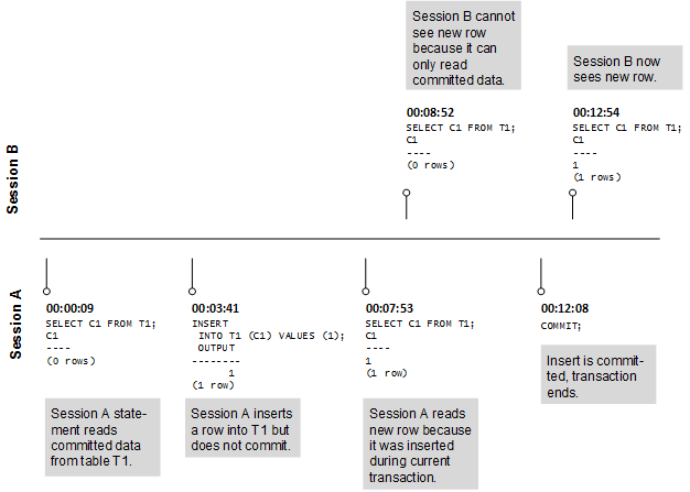
READ COMMITTED isolation maintains exclusive write locks until a transaction ends, as shown in the following graphic:
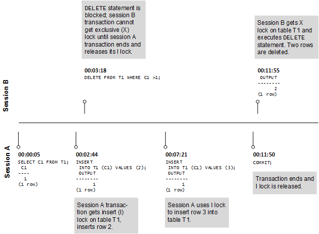
See also
13.4 - SERIALIZABLE isolation
SERIALIZABLE is the strictest SQL transaction isolation level.
SERIALIZABLE is the strictest SQL transaction isolation level. While this isolation level permits transactions to run concurrently, it creates the effect that transactions are running in serial order. Transactions acquire locks for read and write operations. Thus, successive SELECT commands within a single transaction always produce the same results. Because SERIALIZABLE isolation provides a consistent view of data, it is useful for applications that require complex queries and updates. However, serializable isolation reduces concurrency. For example, it blocks queries during a bulk load.
SERIALIZABLE isolation establishes the following locks:
-
Table-level read locks: Vertica acquires table-level read locks on selected tables and releases them when the transaction ends. This behavior prevents one transaction from modifying rows while they are being read by another transaction.
-
Table-level write lock: Vertica acquires table-level write locks on update and releases them when the transaction ends. This behavior prevents one transaction from reading another transaction's changes to rows before those changes are committed.
At the start of a transaction, a SELECT statement obtains a backup of the selection's committed data. The transaction also sees the results of updates that are run within the transaction before they are committed.
The following figure shows how concurrent transactions that both have SERIALIZABLE isolation levels handle locking:
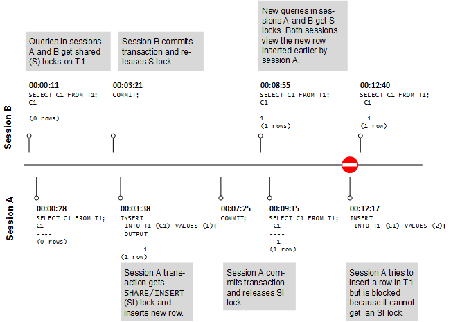
Applications that use SERIALIZABLE must be prepared to retry transactions due to serialization failures. Such failures often result from deadlocks. When a deadlock occurs, any transaction awaiting a lock automatically times out after 5 minutes. The following figure shows how deadlock might occur and how Vertica handles it:
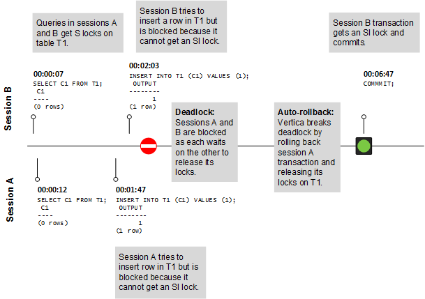
Note
SERIALIZABLE isolation does not apply to temporary tables. No locks are required for these tables because they are isolated by their transaction scope.
See also Vertica
14 - Vertica database locks
When multiple users concurrently access the same database information, data manipulation can cause conflicts and threaten data integrity.
When multiple users concurrently access the same database information, data manipulation can cause conflicts and threaten data integrity. Conflicts occur because some transactions block other operations until the transaction completes. Because transactions committed at the same time should produce consistent results, Vertica uses locks to maintain data concurrency and consistency. Vertica automatically controls locking by limiting the actions a user can take on an object, depending on the state of that object.
Vertica uses object locks and system locks. Object locks are used on objects, such as tables and projections. System locks include global catalog locks, local catalog locks, and elastic cluster locks. Vertica supports a full range of standard SQL lock modes, such as shared (S) and exclusive (X).
For related information about lock usage in different transaction isolation levels, see READ COMMITTED isolation and SERIALIZABLE isolation.
14.1 - Lock modes
Vertica has different lock modes that determine how a lock acts on an object.
Vertica has different lock modes that determine how a lock acts on an object. Each lock mode is unique in its compatibility with other lock modes; each lock mode has its own strength vis a vis other lock modes, which determines whether Each lock mode has a lock compatibility and strength that reflect how it interacts with other locks in the same environment.
|
Lock mode |
Description |
|
Usage (U) |
Vertica uses usage (U) locks for Tuple Mover mergeout operations. These Tuple Mover operations run automatically in the background, therefore, other operations on a table except those requiring an O or D locks can run when the object is locked in U mode. |
|
Tuple Mover (T) |
Vertica uses Tuple Mover (T) locks for operations on delete vectors. Tuple Mover operations upgrade the table lock mode from U to T when work on delete vectors starts so that no other updates or deletes can happen concurrently. |
|
Shared (S) |
Use a shared (S) lock for SELECT queries that run at the serialized transaction isolation level. This allows queries to run concurrently, but the S lock creates the effect that transactions are running in serial order. The S lock ensures that one transaction does not affect another transaction until one transaction completes and its S lock is released.
Select operations in READ COMMITTED transaction mode do not require S table locks. See Transactions for more information.
|
|
Insert (I) |
Vertica requires an insert (I) lock to insert data into a table. Multiple transactions can lock an object in insert mode simultaneously, enabling multiple inserts and bulk loads to occur at the same time. This behavior is critical for parallel loads and high ingestion rates. |
|
Insert Validate (IV) |
An insert validate (IV) lock is required for insert operations where the system performs constraint validation for enabled PRIMARY or UNIQUE key constraints. |
|
Shared Insert (SI) |
Vertica requires a shared insert (SI) lock when both a read and an insert occur in a transaction. SI mode prohibits delete/update operations. An SI lock also results from lock promotion. |
|
Exclusive (X) |
Vertica uses exclusive (X) locks when performing deletes and updates. Only Tuple Mover mergeout operations (U locks) can run concurrently on objects with X locks. |
|
Drop Partition (D) |
DROP_PARTITIONS requires a D lock on the target table. This lock is only compatible with I-lock operations, so only table load operations such as INSERT and COPY are allowed during drop partition operations. |
|
Owner (O) |
An owner (O) lock is the strongest Vertica lock mode. An object acquires an O lock when it undergoes changes in both data and structure. Such changes can occur in some DDL operations, such as DROP_PARTITIONS, TRUNCATE TABLE, and ADD COLUMN. When an object is locked in O mode, it cannot be locked simultaneously by another transaction in any mode. |
Lock compatibility
Bulleted (•) cells in the following matrix shows which locks can be used on the same object simultaneously. Empty cells indicate that a query's requested mode is not granted until the current (granted) mode releases its lock on the object.
|
Requested mode |
Granted mode |
|
U |
T |
S |
I |
IV |
SI |
X |
D |
O |
|
U |
• |
• |
• |
• |
• |
• |
• |
|
|
|
T |
• |
• |
• |
• |
• |
• |
|
|
|
|
S |
• |
• |
• |
|
|
|
|
|
|
|
I |
• |
• |
|
• |
• |
|
|
• |
|
|
IV |
• |
• |
|
• |
|
|
|
|
|
|
SI |
• |
• |
|
|
|
|
|
|
|
|
X |
• |
|
|
|
|
|
|
|
|
|
D |
|
|
|
• |
|
|
|
|
|
|
O |
|
|
|
|
|
|
|
|
|
Lock conversion
Often, the same object is the target of concurrent lock requests from different sessions. The matrix below shows how Vertica responds to multiple lock requests on the same object, one of the following:
- Locks are granted to concurrent requests on an object if the respective lock modes are compatible. For example, D (drop partition) and I (insert) locks are compatible, so Vertica can grant multiple lock requests on the same table for concurrent load and drop partition operations.
- Lock modes for concurrent requests on an object are incompatible, but the requests also support a higher (stronger) lock mode. In this case, Vertica converts (upgrades) the lock modes for these requests—for example, S and I to SI. The upgraded lock mode enables requests on the object to proceed concurrently.
- Lock modes for concurrent requests on an object are incompatible, and none can be upgraded to a common lock mode. In this case, object lock requests are queued and granted in sequence.
|
Requested mode |
Granted mode |
|
U |
T |
S |
I |
IV |
SI |
X |
D |
O |
|
U |
U |
T |
S |
I |
IV |
SI |
X |
D |
O |
|
T |
T |
T |
S |
I |
IV |
SI |
X |
D |
O |
|
S |
S |
S |
S |
SI |
SI |
SI |
X |
O |
O |
|
I |
I |
I |
SI |
I |
IV |
SI |
X |
D |
O |
|
IV |
IV |
IV |
SI |
IV |
IV |
SI |
X |
D |
O |
|
SI |
SI |
SI |
SI |
SI |
SI |
SI |
X |
O |
O |
|
X |
X |
X |
X |
X |
X |
X |
X |
O |
O |
|
D |
D |
D |
O |
D |
D |
O |
O |
D |
O |
|
O |
O |
O |
O |
O |
O |
O |
O |
O |
O |
Lock strength
Lock strength refers to the ability of a lock mode to interact with another lock mode. O locks are strongest and are incompatible with all other locks. Conversely, U locks are weakest and can run concurrently with all other locks except D and O locks.
The following figure depicts the spectrum of lock mode strength:
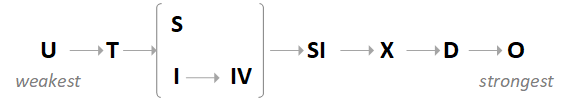
See also
14.2 - Lock examples
In this example, two sessions (A and B) attempt to perform operations on table T1.
Automatic locks
In this example, two sessions (A and B) attempt to perform operations on table T1. These operations automatically acquire the necessary locks.
At the beginning of the example, table T1 has one column (C1) and no rows.
The steps here represent a possible series of transactions from sessions A and B:
-
Transactions in both sessions acquire S locks to read from Table T1.
-
Session B releases its S lock with the COMMIT statement.
-
Session A can upgrade to an SI lock and insert into T1 because Session B released its S lock.
-
Session A releases its SI lock with a COMMIT statement.
-
Both sessions can acquire S locks because Session A released its SI lock.
-
Session A cannot acquire an SI lock because Session B has not released its S lock. SI locks are incompatible with S locks.
-
Session B releases its S lock with the COMMIT statement.
-
Session A can now upgrade to an SI lock and insert into T1.
-
Session B attempts to delete a row from T1 but can't acquire an X lock because Session A has not released its SI lock. SI locks are incompatible with X locks.
-
Session A continues to insert into T1.
-
Session A releases its SI lock.
-
Session B can now acquire an X lock and perform the delete.
This figure illustrates the previous steps:
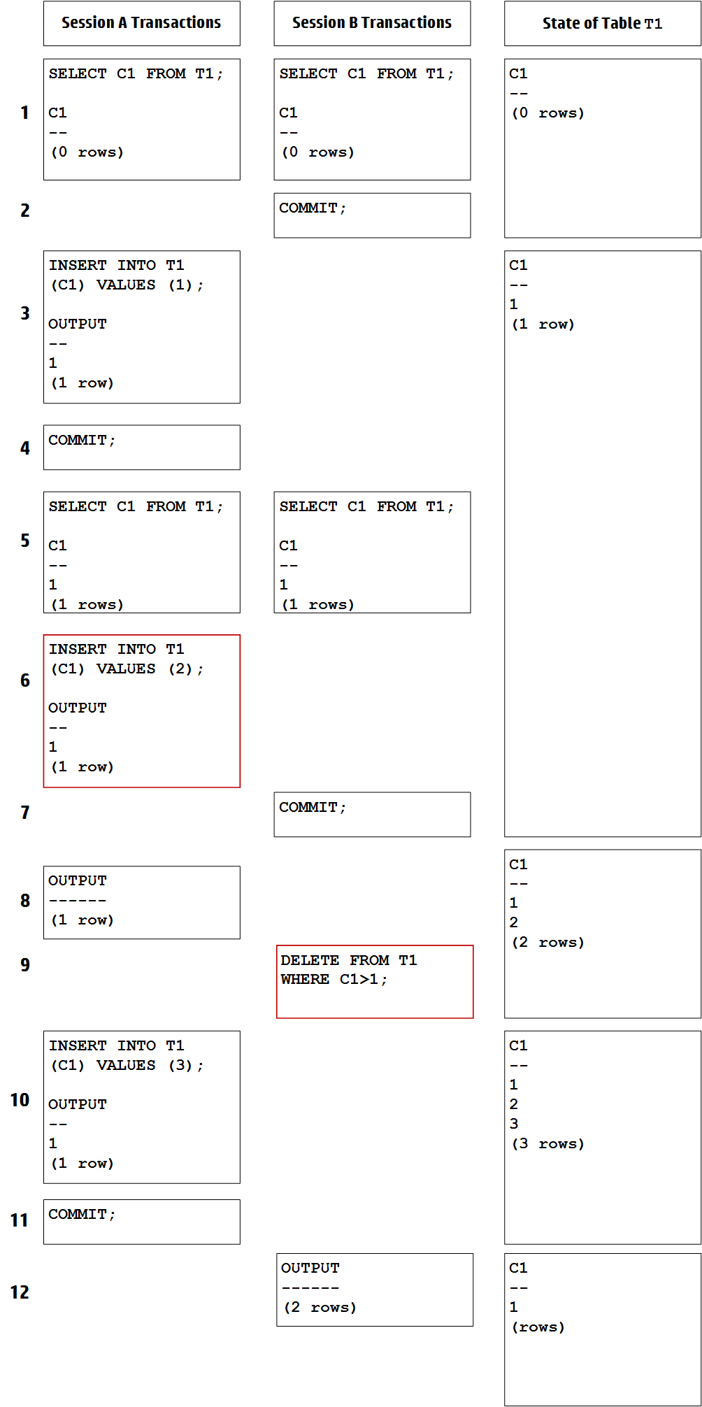
Manual locks
In this example, Alice attempts to manually lock table customer_info with LOCK TABLE while Bob runs an INSERT statement:
Bob runs the following INSERT statement to acquire an INSERT lock and insert a row:
=> INSERT INTO customer_info VALUES(37189,'Albert','Quinlan','Frankfurt',2022);
In another session, Alice attempts to acquire a SHARE lock with LOCK TABLE. As shown in the lock compatibility table, the INSERT lock is incompatible with SHARE locks (among others), so Alice cannot acquire a SHARE lock until Bob finishes his transaction:
=> LOCK customer_info IN SHARE MODE NOWAIT;
ERROR 5157: Unavailable: [Txn 0xa00000001c48e3] S lock table - timeout error Timed out S locking Table:public.customer_info. I held by [user Bob (LOCK TABLE)]. Your current transaction isolation level is READ COMMITTED
Bob then releases the lock by calling COMMIT:
=> COMMIT;
COMMIT
Alice can now acquire the SHARE lock:
=> LOCK customer_info IN SHARE MODE NOWAIT;
LOCK TABLE
Bob tries to insert another row into the table, but because Alice has the SHARE lock, the statement enters a queue and appears to hang; after Alice finishes her transaction, the INSERT statement will automatically acquire the INSERT lock:
=> INSERT INTO customer_info VALUES(17441,'Kara','Shen','Cairo',2022);
Alice calls COMMIT, ending her transaction and releasing the SHARE lock:
=> COMMIT;
COMMIT;
Bob's INSERT statement automatically acquires the lock and completes the operation:
=> INSERT INTO customer_info VALUES(17441,'Kara','Shen','Cairo',2022);
OUTPUT
--------
1
(1 row)
Bob calls COMMIT, ending his transaction and releasing the INSERT lock:
=> COMMIT;
COMMIT
14.3 - Deadlocks
Deadlocks can occur when two or more sessions with locks on a table attempt to elevate to lock types incompatible with the lock owned by another session.
Deadlocks can occur when two or more sessions with locks on a table attempt to elevate to lock types incompatible with the lock owned by another session. For example, suppose Bob and Alice each run an INSERT statement:
--Alice's session
=> INSERT INTO customer_info VALUES(92837,'Alexander','Lamar','Boston',2022);
--Bob's session
=> INSERT INTO customer_info VALUES(76658,'Midori','Tanaka','Osaka',2021);
INSERT (I) locks are compatible, so both Alice and Bob have the lock:
=> SELECT * FROM locks;
-[ RECORD 1 ]-----------+-------------------------------------------------------------------------------------------------
node_names | v_vmart_node0001,v_vmart_node0002,v_vmart_node0003
object_name | Table:public.customer_info
object_id | 45035996274212656
transaction_id | 45035996275578544
transaction_description | Txn: a00000001c96b0 'INSERT INTO customer_info VALUES(92837,'Alexander','Lamar','Boston',2022);'
lock_mode | I
lock_scope | TRANSACTION
request_timestamp | 2022-10-05 12:57:49.039967-04
grant_timestamp | 2022-10-05 12:57:49.039971-04
-[ RECORD 2 ]-----------+-------------------------------------------------------------------------------------------------
node_names | v_vmart_node0001,v_vmart_node0002,v_vmart_node0003
object_name | Table:public.customer_info
object_id | 45035996274212656
transaction_id | 45035996275578546
transaction_description | Txn: a00000001c96b2 'INSERT INTO customer_info VALUES(76658,'Midori','Tanaka','Osaka',2021);'
lock_mode | I
lock_scope | TRANSACTION
request_timestamp | 2022-10-05 12:57:56.599637-04
grant_timestamp | 2022-10-05 12:57:56.599641-04
Alice then runs an UPDATE statement, attempting to elevate her existing INSERT lock into an EXCLUSIVE (X) lock. However, because EXCLUSIVE locks are incompatible with the INSERT lock in Bob's session, the UPDATE is added to a queue for the lock and appears to hang:
=> UPDATE customer_info SET city='Cambridge' WHERE customer_id=92837;
A deadlock occurs when Bob runs an UPDATE statement while Alice's UPDATE is still waiting. Vertica detects the deadlock and terminates Bob's entire transaction (which includes his INSERT), allowing Alice to elevate to an EXCLUSIVE lock and complete her UPDATE:
=> UPDATE customer_info SET city='Shibuya' WHERE customer_id=76658;
ROLLBACK 3010: Deadlock: initiator locks for query - Deadlock X locking Table:public.customer_info. I held by [user Alice (INSERT INTO customer_info VALUES(92837,'Alexander','Lamar','Boston',2022);)]. Your current transaction isolation level is SERIALIZABLE
Preventing deadlocks
You can avoid deadlocks by acquiring the elevated lock earlier in the transaction, ensuring that your session has exclusive access to the table. You can do this in several ways:
To prevent a deadlock in the previous example, Alice and Bob should both begin their transactions with LOCK TABLE. The first session to request the lock will lock the table, and the other waits for the first session to release the lock or until a user-specified timeout:
=> LOCK TABLE customer_info IN EXCLUSIVE MODE;
14.4 - Troubleshooting locks
The LOCKS and LOCK_USAGE system tables can help identify problems you may encounter with Vertica database locks.
The LOCKS and LOCK_USAGE system tables can help identify problems you may encounter with Vertica database locks.
This example shows one row from the LOCKS system table. From this table you can see what types of locks are active on specific objects and nodes.
=> SELECT node_names, object_name, lock_mode, lock_scope FROM LOCKS;
node_names | object_name | lock_mode | lock_scope
-------------------+---------------------------------+-----------+-----------
v_vmart_node0001 | Table:public.customer_dimension | X | TRANSACTION
This example shows two rows from the LOCKS_USAGE system table. You can also use this table to see what locks are in use on specific objects and nodes.
=> SELECT node_name, object_name, mode FROM LOCK_USAGE;
node_name | object_name | mode
------------------+------------------+-------
v_vmart_node0001 | Cluster Topology | S
v_vmart_node0001 | Global Catalog | X
15 - Using text search
Text search allows you to quickly search the contents of a single CHAR, VARCHAR, LONG VARCHAR, VARBINARY, or LONG VARBINARY field within a table to locate a specific keyword.
Text search allows you to quickly search the contents of a single CHAR, VARCHAR, LONG VARCHAR, VARBINARY, or LONG VARBINARY field within a table to locate a specific keyword.
You can use this feature on columns that are queried repeatedly regarding their contents. After you create the text index, DML operations become slightly slower on the source table. This performance change results from syncing the text index and source table. Any time an operation is performed on the source table, the text index updates in the background. Regular queries on the source table are not affected.
The text index contains all of the words from the source table's text field and any other additional columns you included during index creation. Additional columns are not indexed—their values are just passed through to the text index. The text index is like any other Vertica table , except it is linked to the source table internally.
First, create a text index on the table you plan to search. Then, after you have indexed your table, run a query against the text index for a specific keyword. This query returns a doc_id for each instance of the keyword. After querying the text index, joining the text index back to the source table should give a significant performance improvement over directly querying the source table about the contents of its text field.
Important
Do not alter the contents or definitions of the text index. If you alter the contents or definitions of the text index, the results do not appropriately match the source table.
15.1 - Creating a text index
In the following example, you perform a text search using a source table called t_log.
In the following example, you perform a text search using a source table called t_log. This source table has two columns:
You must associate a projection with the source table. Use a projection that is sorted by the primary key and either segmented by hash(id) or unsegmented. You can define this projection on the source table, along with any other existing projections.
Create a text index on the table for which you want to perform a text search.
=> CREATE TEXT INDEX text_index ON t_log (id, text);
The text index contains two columns:
-
doc_id uses the unique identifier from the source table.
-
token is populated with text strings from the designated column from the source table. The word column results from tokenizing and stemming the words found in the text column.
If your table is partitioned then your text index also contains a third column named partition.
=> SELECT * FROM text_index;
token | doc_id | partition
------------------------+--------+-----------
<info> | 6 | 2014
<warning> | 2 | 2014
<warning> | 3 | 2014
<warning> | 4 | 2014
<warning> | 5 | 2014
database | 6 | 2014
execute: | 6 | 2014
object | 4 | 2014
object | 5 | 2014
[catalog] | 4 | 2014
[catalog] | 5 | 2014
You create a text index on a source table only once. In the future, you do not have to re-create the text index each time the source table is updated or changed.
Your text index stays synchronized to the contents of the source table through any operation that is run on the source table. These operations include, but are not limited to:
15.2 - Creating a text index on a flex table
In the following example, you create a text index on a flex table.
In the following example, you create a text index on a flex table. The example assumes that you have created a flex table called mountains. See Getting started in Using Flex Tables to create the flex table used in this example.
Before you can create a text index on your flex table, add a primary key constraint to the flex table.
=> ALTER TABLE mountains ADD PRIMARY KEY (__identity__);
Create a text index on the table for which you want to perform a text search. Tokenize the __raw__column with the FlexTokenizer and specify the data type as LONG VARBINARY. It is important to use the FlexTokenizer when creating text indices on flex tables because the data type of the __raw__ column differs from the default StringTokenizer.
=> CREATE TEXT INDEX flex_text_index ON mountains(__identity__, __raw__) TOKENIZER public.FlexTokenizer(long varbinary);
The text index contains two columns:
-
doc_id uses the unique identifier from the source table.
-
token is populated with text strings from the designated column from the source table. The word column results from tokenizing and stemming the words found in the text column.
If your table is partitioned then your text index also contains a third column named partition.
=> SELECT * FROM flex_text_index;
token | doc_id
-------------+--------
50.6 | 5
Mt | 5
Washington | 5
mountain | 5
12.2 | 3
15.4 | 2
17000 | 3
29029 | 2
Denali | 3
Helen | 2
Mt | 2
St | 2
mountain | 3
volcano | 2
29029 | 1
34.1 | 1
Everest | 1
mountain | 1
14000 | 4
Kilimanjaro | 4
mountain | 4
(21 rows)
You create a text index on a source table only once. In the future, you do not have to re-create the text index each time the source table is updated or changed.
Your text index stays synchronized to the contents of the source table through any operation that is run on the source table. These operations include, but are not limited to:
15.3 - Searching a text index
After you create a text index, write a query to run against the index to search for a specific keyword.
After you create a text index, write a query to run against the index to search for a specific keyword.
In the following example, you use a WHERE clause to search for the keyword <WARNING> in the text index. The WHERE clause should use the stemmer you used to create the text index. When you use the STEMMER keyword, it stems the keyword to match the keywords in your text index. If you did not use the STEMMER keyword, then the default stemmer is v_txtindex.StemmerCaseInsensitive. If you used STEMMER NONE, then you can omit STEMMER keyword from the WHERE clause.
=> SELECT * FROM text_index WHERE token = v_txtindex.StemmerCaseInsensitive('<WARNING>');
token | doc_id
-----------+--------
<warning> | 2
<warning> | 3
<warning> | 4
<warning> | 5
(4 rows)
Next, write a query to display the full contents of the source table that match the keyword you searched for in the text index.
=> SELECT * FROM t_log WHERE id IN (SELECT doc_id FROM text_index WHERE token = v_txtindex.StemmerCaseInsensitive('<WARNING>'));
id | date | text
---+------------+-----------------------------------------------------------------------------------------------
4 | 2014-06-04 | 11:00:49.568 unknown:0x7f9207607700 [Catalog] <WARNING> validateDependencies: Object 45035968
5 | 2014-06-04 | 11:00:49.568 unknown:0x7f9207607700 [Catalog] <WARNING> validateDependencies: Object 45030
2 | 2013-06-04 | 11:00:49.568 unknown:0x7f9207607700 [Catalog] <WARNING> validateDependencies: Object 4503
3 | 2013-06-04 | 11:00:49.568 unknown:0x7f9207607700 [Catalog] <WARNING> validateDependencies: Object 45066
(4 rows)
Use the doc_id to find the exact location of the keyword in the source table.The doc_id matches the unique identifier from the source table. This matching allows you to quickly find the instance of the keyword in your table.
Performing a case-sensitive and case-insensitive text search query
Your text index is optimized to match all instances of words depending upon your stemmer. By default, the case insensitive stemmer is applied to all text indices that do not specify a stemmer. Therefore, if the queries you plan to write against your text index are case sensitive, then Vertica recommends you use a case sensitive stemmer to build your text index.
The following examples show queries that match case-sensitive and case-insensitive words that you can use when performing a text search.
This query finds case-insensitive records in a case insensitive text index:
=> SELECT * FROM t_log WHERE id IN (SELECT doc_id FROM text_index WHERE token = v_txtindex.StemmerCaseInsensitive('warning'));
This query finds case-sensitive records in a case sensitive text index:
=> SELECT * FROM t_log_case_sensitive WHERE id IN (SELECT doc_id FROM text_index WHERE token = v_txtindex.StemmerCaseSensitive('Warning'));
Including and excluding keywords in a text search query
Your text index also allows you to perform more detailed queries to find multiple keywords or omit results with other keywords. The following example shows a more detailed query that you can use when performing a text search.
In this example, t_log is the source table, and text_index is the text index. The query finds records that either contain:
SELECT * FROM t_log where (
id IN (SELECT doc_id FROM text_index WHERE token = v_txtindex.StemmerCaseSensitive('<WARNING>'))
AND ( id IN (SELECT doc_id FROM text_index WHERE token = v_txtindex.StemmerCaseSensitive('validate')
OR id IN (SELECT doc_id FROM text_index WHERE token = v_txtindex.StemmerCaseSensitive('[Log]')))
AND NOT (id IN (SELECT doc_id FROM text_index WHERE token = v_txtindex.StemmerCaseSensitive('validateDependencies'))));
This query returns the following results:
id | date | text
----+------------+------------------------------------------------------------------------------------------------
11 | 2014-05-04 | 11:00:49.568 unknown:0x7f9207607702 [Log] <WARNING> validate: Object 4503 via fld num_all_roles
13 | 2014-05-04 | 11:00:49.568 unknown:0x7f9207607706 [Log] <WARNING> validate: Object 45035 refers to root_i3
14 | 2014-05-04 | 11:00:49.568 unknown:0x7f9207607708 [Log] <WARNING> validate: Object 4503 refers to int_2
17 | 2014-05-04 | 11:00:49.568 unknown:0x7f9207607700 [Txn] <WARNING> Begin validate Txn: fff0ed17 catalog editor
(4 rows)
15.4 - Dropping a text index
Dropping a text index removes the specified text index from the database.
Dropping a text index removes the specified text index from the database.
You can drop a text index when:
Dropping the text index does not drop the source table associated with the text index. However, if you drop the source table associated with a text index, then that text index is also dropped. Vertica considers the text index a dependent object.
The following example illustrates how to drop a text index named text_index:
=> DROP TEXT INDEX text_index;
DROP INDEX
15.5 - Stemmers and tokenizers
Vertica provides default stemmers and tokenizers.
Vertica provides default stemmers and tokenizers. You can also create your own custom stemmers and tokenizers. The following topics explain the default stemmers and tokenizers, and the requirements for creating custom stemmers and tokenizers in Vertica.
15.5.1 - Vertica stemmers
Vertica stemmers use the Porter stemming algorithm to find words derived from the same base/root word.
Vertica stemmers use the Porter stemming algorithm to find words derived from the same base/root word. For example, if you perform a search on a text index for the keyword database, you might also want to get results containing the word databases.
To achieve this type of matching, Vertica stores words in their stemmed form when using any of the v_txtindex stemmers.
The Vertica Analytics Platform provides the following stemmers:
|
Name |
Description |
|
v_txtindex.Stemmer(long varchar) |
Not sensitive to case; outputs lowercase words. Stems strings from a Vertica table.
Alias of StemmerCaseInsensitive.
|
|
v_txtindex.StemmerCaseSensitive(long varchar) |
Sensitive to case. Stems strings from a Vertica table. |
|
v_txtindex.StemmerCaseInsensitive(long varchar) |
Default stemmer used if no stemmer is specified when creating a text index.
Not sensitive to case; outputs lowercase words. Stems strings from a Vertica table.
|
|
v_txtindex.caseInsensitiveNoStemming(long varchar) |
Not sensitive to case; outputs lowercase words. Does not use the Porter Stemming algorithm. |
Examples
The following examples show how to use a stemmer when creating a text index.
Create a text index using the StemmerCaseInsensitive stemmer:
=> CREATE TEXT INDEX idx_100 ON top_100 (id, feedback) STEMMER v_txtindex.StemmerCaseInsensitive(long varchar)
TOKENIZER v_txtindex.StringTokenizer(long varchar);
Create a text index using the StemmerCaseSensitive stemmer:
=> CREATE TEXT INDEX idx_unstruc ON unstruc_data (__identity__, __raw__) STEMMER v_txtindex.StemmerCaseSensitive(long varchar)
TOKENIZER public.FlexTokenizer(long varbinary);
Create a text index without using a stemmer:
=> CREATE TEXT INDEX idx_logs FROM sys_logs ON (id, message) STEMMER NONE TOKENIZER v_txtindex.StringTokenizer(long varchar);
15.5.2 - Vertica tokenizers
A tokenizer does the following:.
A tokenizer does the following:
-
Receives a stream of characters.
-
Breaks the stream into individual tokens that usually correspond to individual words.
-
Returns a stream of tokens.
15.5.2.1 - Preconfigured tokenizers
The Vertica Analytics Platform provides the following preconfigured tokenizers:.
The Vertica Analytics Platform provides the following preconfigured tokenizers:
|
Name |
Description |
|
public.FlexTokenizer(LONG VARBINARY) |
Splits the values in your flex table by white space. |
|
v_txtindex.StringTokenizer(LONG VARCHAR) |
Splits the string into words by splitting on white space. |
v_txtindex.StringTokenizerDelim(string LONG VARCHAR, 'delimiter' CHAR(1)) |
Splits a string into tokens using the specified delimiter character. |
|
v_txtindex.AdvancedLogTokenizer |
Uses the default parameters for all tokenizer parameters. For more information, see Advanced log tokenizer. |
|
v_txtindex.BasicLogTokenizer |
Uses the default values for all tokenizer parameters except minorseparator, which is set to an empty list. For more information, see Basic log tokenizer. |
|
v_txtindex.WhitespaceLogTokenizer |
Uses default values for tokenizer parameters, except for majorseparators, which uses E' \t\n\f\r'; and minorseparator, which uses an empty list. For more information, see Whitespace log tokenizer. |
Vertica also provides the following tokenizer, which is not preconfigured:
|
Name |
Description |
|
v_txtindex.ICUTokenizer |
Supports multiple languages. Tokenizes based on the conventions of the language you set in the locale parameter. For more information, see ICU Tokenizer. |
Examples
The following examples show how you can use a preconfigured tokenizer when creating a text index.
Use the StringTokenizer to create an index from the top_100:
=> CREATE TEXT INDEX idx_100 FROM top_100 on (id, feedback)
TOKENIZER v_txtindex.StringTokenizer(long varchar)
STEMMER v_txtindex.StemmerCaseInsensitive(long varchar);
Use the FlexTokenizer to create an index from unstructured data:
=> CREATE TEXT INDEX idx_unstruc FROM unstruc_data on (__identity__, __raw__)
TOKENIZER public.FlexTokenizer(long varbinary)
STEMMER v_txtindex.StemmerCaseSensitive(long varchar);
Use the StringTokenizerDelim to split a string at the specified delimiter:
=> CREATE TABLE string_table (word VARCHAR(100), delim VARCHAR);
CREATE TABLE
=> COPY string_table FROM STDIN DELIMITER ',';
Enter data to be copied followed by a newline.
End with a backslash and a period on a line by itself.
>>
>> SingleWord,dd
>> Break On Spaces,' '
>> Break:On:Colons,:
>> \.
=> SELECT * FROM string_table;
word | delim
-----------------+-------
SingleWord | dd
Break On Spaces |
Break:On:Colons | :
(3 rows)
=> SELECT v_txtindex.StringTokenizerDelim(word,delim) OVER () FROM string_table;
words
-----------------
Break
On
Colons
SingleWor
Break
On
Spaces
(7 rows)
=> SELECT v_txtindex.StringTokenizerDelim(word,delim) OVER (PARTITION BY word), word as input FROM string_table;
words | input
-----------------+-----------------
Break | Break:On:Colons
On | Break:On:Colons
Colons | Break:On:Colons
SingleWor | SingleWord
Break | Break On Spaces
On | Break On Spaces
Spaces | Break On Spaces
(7 rows)
15.5.2.2 - Advanced log tokenizer
Returns tokens that can include minor separators.
Returns tokens that can include minor separators. You can use this tokenizer in situations when your tokens are separated by whitespace or various punctuation. The advanced log tokenizer offers more granularity than the basic log tokenizer in defining separators through the addition of minor separators. This approach is frequently appropriate for analyzing log files.
Important
If you create a database with no tables and the k-safety has increased, you must rebalance your data using
REBALANCE_CLUSTER before using a Vertica tokenizer.
Parameters
|
Parameter Name |
Parameter Value |
|
stopwordscaseinsensitive |
'' |
|
minorseparators |
E'/:=@.-$#%\\_' |
|
majorseparators |
E' []<>(){}|!;,''"*&?+\r\n\t' |
|
minLength |
'2' |
|
maxLength |
'128' |
|
used |
'True' |
Examples
The following example shows how you can create a text index, from the table foo, using the Advanced Log Tokenizer without a stemmer.
=> CREATE TABLE foo (id INT PRIMARY KEY NOT NULL,text VARCHAR(250));
=> COPY foo FROM STDIN;
End with a backslash and a period on a line by itself.
>> 1|2014-05-10 00:00:05.700433 %ASA-6-302013: Built outbound TCP connection 9986454 for outside:101.123.123.111/443 (101.123.123.111/443)
>> \.
=> CREATE PROJECTION foo_projection AS SELECT * FROM foo ORDER BY id
SEGMENTED BY HASH(id) ALL NODES KSAFE;
=> CREATE TEXT INDEX indexfoo_AdvancedLogTokenizer ON foo (id, text)
TOKENIZER v_txtindex.AdvancedLogTokenizer(LONG VARCHAR) STEMMER NONE;
=> SELECT * FROM indexfoo_AdvancedLogTokenizer;
token | doc_id
-----------------------------+--------
%ASA-6-302013: | 1
00 | 1
00:00:05.700433 | 1
05 | 1
10 | 1
101 | 1
101.123.123.111/443 | 1
111 | 1
123 | 1
2014 | 1
2014-05-10 | 1
302013 | 1
443 | 1
700433 | 1
9986454 | 1
ASA | 1
Built | 1
TCP | 1
connection | 1
for | 1
outbound | 1
outside | 1
outside:101.123.123.111/443 | 1
(23 rows)
15.5.2.3 - Basic log tokenizer
Returns tokens that exclude specified minor separators.
Returns tokens that exclude specified minor separators. You can use this tokenizer in situations when your tokens are separated by whitespace or various punctuation. This approach is frequently appropriate for analyzing log files.
Important
If you create a database with no tables and the k-safety has increased, you must rebalance your data using
REBALANCE_CLUSTER before using a Vertica tokenizer.
Parameters
|
Parameter Name |
Parameter Value |
|
stopwordscaseinsensitive |
'' |
|
minorseparators |
'' |
|
majorseparators |
E' []<>(){}|!;,''"*&?+\r\n\t' |
|
minLength |
'2' |
|
maxLength |
'128' |
|
used |
'True' |
Examples
The following example shows how you can create a text index, from the table foo, using the Basic Log Tokenizer without a stemmer.
=> CREATE TABLE foo (id INT PRIMARY KEY NOT NULL,text VARCHAR(250));
=> COPY foo FROM STDIN;
End with a backslash and a period on a line by itself.
>> 1|2014-05-10 00:00:05.700433 %ASA-6-302013: Built outbound TCP connection 9986454 for outside:101.123.123.111/443 (101.123.123.111/443)
>> \.
=> CREATE PROJECTION foo_projection AS SELECT * FROM foo ORDER BY id
SEGMENTED BY HASH(id) ALL NODES KSAFE;
=> CREATE TEXT INDEX indexfoo_BasicLogTokenizer ON foo (id, text)
TOKENIZER v_txtindex.BasicLogTokenizer(LONG VARCHAR) STEMMER NONE;
=> SELECT * FROM indexfoo_BasicLogTokenizer;
token | doc_id
-----------------------------+--------
%ASA-6-302013: | 1
00:00:05.700433 | 1
101.123.123.111/443 | 1
2014-05-10 | 1
9986454 | 1
Built | 1
TCP | 1
connection | 1
for | 1
outbound | 1
outside:101.123.123.111/443 | 1
(11 rows)
15.5.2.4 - Whitespace log tokenizer
Returns only tokens surrounded by whitespace.
Returns only tokens surrounded by whitespace. You can use this tokenizer in situations where you want to the tokens in your source document to be separated by whitespace characters only. This approach lets you retain the ability to set stop words and token length limits.
Important
If you create a database with no tables and the k-safety has increased, you must rebalance your data using
REBALANCE_CLUSTER before using a Vertica tokenizer.
Parameters
|
Parameter Name |
Parameter Value |
|
stopwordscaseinsensitive |
'' |
|
minorseparators |
'' |
|
majorseparators |
E' \t\n\f\r' |
|
minLength |
'2' |
|
maxLength |
'128' |
|
used |
'True' |
Examples
The following example shows how you can create a text index, from the table foo, using the Whitespace Log Tokenizer without a stemmer.
=> CREATE TABLE foo (id INT PRIMARY KEY NOT NULL,text VARCHAR(250));
=> COPY foo FROM STDIN;
End with a backslash and a period on a line by itself.
>> 1|2014-05-10 00:00:05.700433 %ASA-6-302013: Built outbound TCP connection 998 6454 for outside:101.123.123.111/443 (101.123.123.111/443)
>> \.
=> CREATE PROJECTION foo_projection AS SELECT * FROM foo ORDER BY id
SEGMENTED BY HASH(id) ALL NODES KSAFE;
=> CREATE TEXT INDEX indexfoo_WhitespaceLogTokenizer ON foo (id, text)
TOKENIZER v_txtindex.WhitespaceLogTokenizer(LONG VARCHAR) STEMMER NONE;
=> SELECT * FROM indexfoo_WhitespaceLogTokenizer;
token | doc_id
-----------------------------+--------
%ASA-6-302013: | 1
(101.123.123.111/443) | 1
00:00:05.700433 | 1
2014-05-10 | 1
6454 | 1
998 | 1
Built | 1
TCP | 1
connection | 1
for | 1
outbound | 1
outside:101.123.123.111/443 | 1
(12 rows)
15.5.2.5 - ICU tokenizer
Supports multiple languages.
Supports multiple languages. You can use this tokenizer to identify word boundaries in languages other than English, including Asian languages that are not separated by whitespace.
The ICU Tokenizer is not pre-configured. You configure the tokenizer by first creating a user-defined transform Function (UDTF). Then set the parameter, locale, to identify the language to tokenizer.
Important
If you create a database with no tables and the k-safety has increased, you must rebalance your data using
REBALANCE_CLUSTER before using a Vertica tokenizer.
Parameters
|
Parameter Name |
Parameter Value |
|
locale |
Uses the POSIX naming convention: language[_COUNTRY]
Identify the language using its ISO-639 code, and the country using its ISO-3166 code. For example, the parameter value for simplified Chinese is zh_CN, and the value for Spanish is es_ES.
The default value is English if you do not specify a locale.
|
Example
The following example steps show how you can configure the ICU Tokenizer for simplified Chinese, then create a text index from the table foo, which contains Chinese characters.
For more on how to configure tokenizers, see Configuring a tokenizer.
-
Create the tokenizer using a UDTF. The example tokenizer is named ICUChineseTokenizer.
VMart=> CREATE OR REPLACE TRANSFORM FUNCTION v_txtindex.ICUChineseTokenizer AS LANGUAGE 'C++' NAME 'ICUTokenizerFactory' LIBRARY v_txtindex.logSearchLib NOT FENCED;
CREATE TRANSFORM FUNCTION
-
Get the procedure ID of the tokenizer.
VMart=> SELECT proc_oid from vs_procedures where procedure_name = 'ICUChineseTokenizer';
proc_oid
-------------------
45035996280452894
(1 row)
-
Set the parameter, locale, to simplified Chinese. Identify the tokenizer using its procedure ID.
VMart=> SELECT v_txtindex.SET_TOKENIZER_PARAMETER('locale','zh_CN' using parameters proc_oid='45035996280452894');
SET_TOKENIZER_PARAMETER
-------------------------
t
(1 row)
-
Lock the tokenizer.
VMart=> SELECT v_txtindex.SET_TOKENIZER_PARAMETER('used','true' using parameters proc_oid='45035996273762696');
SET_TOKENIZER_PARAMETER
-------------------------
t
(1 row)
-
Create an example table, foo, containing simplified Chinese text to index.
VMart=> CREATE TABLE foo(doc_id integer primary key not null,text varchar(250));
CREATE TABLE
VMart=> INSERT INTO foo values(1, u&'\4E2D\534E\4EBA\6C11\5171\548C\56FD');
OUTPUT
--------
1
-
Create an index, index_example, on the table foo. The example creates the index without a stemmer; Vertica stemmers work only on English text. Using a stemmer for English on non-English text can cause incorrect tokenization.
VMart=> CREATE TEXT INDEX index_example ON foo (doc_id, text) TOKENIZER v_txtindex.ICUChineseTokenizer(long varchar) stemmer none;
CREATE INDEX
-
View the new index.
VMart=> SELECT * FROM index_example ORDER BY token,doc_id;
token | doc_id
--------+--------
中华 | 1
人民 | 1
共和国 | 1
(3 rows)
15.5.3 - Configuring a tokenizer
You configure a tokenizer by creating a user-defined transform function (UDTF) using one of the two base UDTFs in the v_txtindex.AdvTxtSearchLib library.
You configure a tokenizer by creating a user-defined transform function (UDTF) using one of the two base UDTFs in the v_txtindex.AdvTxtSearchLib library. The library contains two base tokenizers: one for Log Words and one for Ngrams. You can configure each base function with or without positional relevance.
15.5.3.1 - Tokenizer base configuration
You can choose among several different tokenizer base configurations:.
You can choose among several different tokenizer base configurations:
|
Type |
Position |
Without Position |
|
Ngram |
logNgramTokenizerPositionFactory |
logNgramTokenizerFactory |
|
Words |
logWordITokenizerPositionFactory |
logWordITokenizerFactory |
Create a logWord tokenizer without positional relevance:
=> CREATE TRANSFORM FUNCTION v_txtindex.fooTokenizer AS LANGUAGE 'C++' NAME 'logWordITokenizerFactory' LIBRARY v_txtindex.logSearchLib NOT FENCED;
15.5.3.2 - RetrieveTokenizerproc_oid
After you create the tokenizer, Vertica writes the name and proc_oid to the system table vs_procedures.
After you create the tokenizer, Vertica writes the name and proc_oid to the system table vs_procedures. You must retrieve the tokenizer's proc_oid to perform additional configuration.
Enter the following query, substituting your own tokenizer name:
=> SELECT proc_oid FROM vs_procedures WHERE procedure_name = 'fooTokenizer';
15.5.3.3 - Set tokenizer parameters
Use the tokenizer's proc_oid to configure the tokenizer.
Use the tokenizer's proc_oid to configure the tokenizer. See Configuring a tokenizer for more information about getting the proc_oid of your tokenizer. The following examples show how you can configure each of the tokenizer parameters:
Configure stop words:
=> SELECT v_txtindex.SET_TOKENIZER_PARAMETER('stopwordscaseinsensitive','for,the' USING PARAMETERS proc_oid='45035996274128376');
Configure major separators:
=> SELECT v_txtindex.SET_TOKENIZER_PARAMETER('majorseparators', E'{}()&[]' USING PARAMETERS proc_oid='45035996274128376');
Configure minor separators:
=> SELECT v_txtindex.SET_TOKENIZER_PARAMETER('minorseparators', '-,$' USING PARAMETERS proc_oid='45035996274128376');
Configure minimum length:
=> SELECT v_txtindex.SET_TOKENIZER_PARAMETER('minlength', '1' USING PARAMETERS proc_oid='45035996274128376');
Configure maximum length:
=> SELECT v_txtindex.SET_TOKENIZER_PARAMETER('maxlength', '140' USING PARAMETERS proc_oid='45035996274128376');
Configure ngramssize:
=> SELECT v_txtindex.SET_TOKENIZER_PARAMETER('ngramssize', '2' USING PARAMETERS proc_oid='45035996274128376');
Lock tokenizer parameters
When you finish configuring the tokenizer, set the parameter, used, to True. After changing this setting, you are no longer able to alter the parameters of the tokenizer. At this point, the tokenizer is ready for you to use to create a text index.
Configure the used parameter:
=> SELECT v_txtindex.SET_TOKENIZER_PARAMETER('used', 'True' USING PARAMETERS proc_oid='45035996274128376');
See also
SET_TOKENIZER_PARAMETER
15.5.3.4 - View tokenizer parameters
After creating a custom tokenizer, you can view the tokenizer's parameter settings in either of two ways:.
After creating a custom tokenizer, you can view the tokenizer's parameter settings in either of two ways:
View individual tokenizer parameter settings
If you need to see an individual parameter setting for a tokenizer, you can use GET_TOKENIZER_PARAMETER to see specific tokenizer parameter settings:
=> SELECT v_txtindex.GET_TOKENIZER_PARAMETER('majorseparators' USING PARAMETERS proc_oid='45035996274126984');
getTokenizerParameter
-----------------------
{}()&[]
(1 row)
For more information, see GET_TOKENIZER_PARAMETER.
View all tokenizer parameter settings
If you need to see all of the parameters for a tokenizer, you can use READ_CONFIG_FILE to see all of the parameter settings for your tokenizer:
=> SELECT v_txtindex.READ_CONFIG_FILE( USING PARAMETERS proc_oid='45035996274126984') OVER();
config_key | config_value
--------------------------+---------------
majorseparators | {}()&[]
maxlength | 140
minlength | 1
minorseparators | -,$
stopwordscaseinsensitive | for,the
type | 1
used | true
(7 rows)
If the parameter, used, is set to False, then you can only view the parameters that have been applied to the tokenizer.
Note
Vertica automatically supplies the value for Type, unless you are using an ngram tokenizer, which allows you to set it.
For more information, see READ_CONFIG_FILE.
15.5.3.5 - Delete tokenizer config file
Use the DELETE_TOKENIZER_CONFIG_FILE function to delete a tokenizer configuration file.
Use the DELETE_TOKENIZER_CONFIG_FILE function to delete a tokenizer configuration file. This function does not delete the User- Defined Transform Function (UDTF). It only deletes the configuration file associated with the UDTF.
Delete the tokenizer configuration file when the parameter, used, is set to False:
=> SELECT v_txtindex.DELETE_TOKENIZER_CONFIG_FILE(USING PARAMETERS proc_oid='45035996274127086');
Delete the tokenizer configuration file with the parameter, confirm, set to True. This setting forces the configuration file deletion, even if the parameter, used, is also set to True:
=> SELECT v_txtindex.DELETE_TOKENIZER_CONFIG_FILE(USING PARAMETERS proc_oid='45035996274126984', confirm='true');
For more information, see DELETE_TOKENIZER_CONFIG_FILE.
15.5.4 - Requirements for custom stemmers and tokenizers
Sometimes, you may want specific tokenization or stemming behavior that differs from what Vertica provides.
Sometimes, you may want specific tokenization or stemming behavior that differs from what Vertica provides. In such cases, you can to implement your own custom User Defined Extensions (UDx) to replace the stemmer or tokenizer. For more information about building custom UDxs see Developing user-defined extensions (UDxs).
Before implementing a custom stemmer or tokenizer in Vertica verify that the UDx extension meets these requirements.
Note
Custom tokenizers can return multi-column text indices.
Vertica stemmer requirements
Comply with these requirements when you create custom stemmers:
-
Must be a User Defined Scalar Function (UDSF) or a SQL Function
-
Can be written in C++, Java, or R
-
Volatility set to stable or immutable
Supported Data Input Types:
Supported Data Output Types:
Vertica tokenizer requirements
To create custom tokenizers, follow these requirements:
-
Must be a User Defined Transform Function (UDTF)
-
Can be written in C++, Java, or R
-
Input type must match the type of the input text
Supported Data Input Types:
-
Char
-
Varchar
-
Long varchar
-
Varbinary
-
Long varbinary
Supported Data Output Types:
16 - Managing storage locations
Vertica are paths to file destinations that you designate to store data and temporary files.
Vertica storage locations are paths to file destinations that you designate to store data and temporary files. Each cluster node requires at least two storage locations: one to store data, and another to store database catalog files. You set up these locations as part of installation and setup. (See
Prepare Disk Storage Locations for disk space requirements.)
Important
Important
While no technical issue prevents you from using CREATE LOCATION to add one or more Network File System (NFS) storage locations, Vertica does not support NFS data or catalog storage except for MapR mount points. You will be unable to run queries against any other NFS data. When creating locations on MapR file systems, you must specify ALL NODES SHARED.
How Vertica uses storage locations
When you add data to the database or perform a DML operation, the new data is added to storage locations on disk as ROS containers. Depending on the configuration of your database, many ROS containers are likely to exist.
You can label the storage locations that you create, in order to reference them for object storage policies. If an object has no storage policy associated with it, Vertica uses default storage algorithms to store its data in available storage locations. If the object has a storage policy, Vertica stores the data at the object's designated storage location. You can can retire or drop store locations when you no longer need them.
Local storage locations
By default, Vertica stores data in unique locations on each node. Each location is in a directory in a file system that the node can access, and is often in the node’s own file system. You can create a local storage location for a single node or for all nodes in the cluster. Cluster-wide storage locations are the most common type of storage. Vertica defaults to using a local cluster-wide storage location for storing all data. If you want it to store data differently, you must create additional storage locations.
Shared storage locations
You can create shared storage locations, where data is stored on a single file system to which all cluster nodes in the cluster have access. This shared file system is often hosted outside of the cluster, such as on a distributed file system like HDFS. Currently, Vertica supports only HDFS shared storage locations. You cannot use NFS as a Vertica shared storage location except when using MapR mount points. See Vertica Storage Location for HDFS for more information.
When you create a shared storage location for DATA and/or TEMP usage, each node in the Vertica cluster creates its own subdirectory in the shared location. The separate directories prevent nodes from overwriting each other's data.
Deprecated
SHARED DATA and SHARED DATA,TEMP storage locations are deprecated.
For databases running in Eon Mode, the STORAGE_LOCATIONS system table shows a third type of location, communal.
16.1 - Viewing storage locations and policies
You can monitor information about available storage location labels and your current storage policies.
You can monitor information about available storage location labels and your current storage policies.
Query the V_MONITOR.DISK_STORAGE system table for disk storage information on each database node. For more information, see Using system tables and Altering location use. The V_MONITOR.DISK_STORAGE system table includes a CATALOG annotation, indicating that the location is used to store catalog files.
Note
You cannot add or remove a catalog storage location. Vertica creates and manages this storage location internally, and the area exists in the same location on each cluster node.
Viewing location labels
Three system tables have information about storage location labels in their location_labels columns:
-
storage_containers
-
storage_locations
-
partitions
Use a query such as the following for relevant columns of the storage_containers system table:
VMART=> select node_name,projection_name, location_label from v_monitor.storage_containers;
node_name | projection_name | location_label
------------------+----------------------+-----------------
v_vmart_node0001 | states_p |
v_vmart_node0001 | states_p |
v_vmart_node0001 | t1_b1 |
v_vmart_node0001 | newstates_b0 | FAST3
v_vmart_node0001 | newstates_b0 | FAST3
v_vmart_node0001 | newstates_b1 | FAST3
v_vmart_node0001 | newstates_b1 | FAST3
v_vmart_node0001 | newstates_b1 | FAST3
.
.
.
Use a query such as the following for columns of the v_catalog.storage_locations system_table:
VMart=> select node_name, location_path, location_usage, location_label from storage_locations;
node_name | location_path | location_usage | location_label
------------------+-------------------------------------------+----------------+----------------
v_vmart_node0001 | /home/dbadmin/VMart/v_vmart_node0001_data | DATA,TEMP |
v_vmart_node0001 | home/dbadmin/SSD/schemas | DATA |
v_vmart_node0001 | /home/dbadmin/SSD/tables | DATA | SSD
v_vmart_node0001 | /home/dbadmin/SSD/schemas | DATA | Schema
v_vmart_node0002 | /home/dbadmin/VMart/v_vmart_node0002_data | DATA,TEMP |
v_vmart_node0002 | /home/dbadmin/SSD/tables | DATA |
v_vmart_node0002 | /home/dbadmin/SSD/schemas | DATA |
v_vmart_node0003 | /home/dbadmin/VMart/v_vmart_node0003_data | DATA,TEMP |
v_vmart_node0003 | /home/dbadmin/SSD/tables | DATA |
v_vmart_node0003 | /home/dbadmin/SSD/schemas | DATA |
(10 rows)
Use a query such as the following for columns of the v_monitor.partitions system table:
VMART=> select partition_key, projection_name, location_label from v_monitor.partitions;
partition_key | projection_name | location_label
---------------+----------------------+---------------
NH | states_b0 | FAST3
MA | states_b0 | FAST3
VT | states_b1 | FAST3
ME | states_b1 | FAST3
CT | states_b1 | FAST3
.
.
.
Viewing storage tiers
Query the storage_tiers system table to see both the labeled and unlabeled storage containers and information about them:
VMart=> select * from v_monitor.storage_tiers;
location_label | node_count | location_count | ros_container_count | total_occupied_size
----------------+------------+----------------+---------------------+---------------------
| 1 | 2 | 17 | 297039391
SSD | 1 | 1 | 9 | 1506
Schema | 1 | 1 | 0 | 0
(3 rows)
Viewing storage policies
Query the storage_policies system table to view the current storage policy in place.
VMART=> select * from v_monitor.storage_policies;
schema_name | object_name | policy_details | location_label
-------------+-------------+------------------+-----------------
| public | Schema | F4
public | lineorder | Partition [4, 4] | M3
(2 rows)
16.2 - Creating storage locations
You can use CREATE LOCATION to add and configure storage locations (other than the required defaults) to provide storage for these purposes:.
You can use CREATE LOCATION to add and configure storage locations (other than the required defaults) to provide storage for these purposes:
-
Isolating execution engine temporary files from data files.
-
Creating labeled locations to use in storage policies.
-
Creating storage locations based on predicted or measured access patterns.
-
Creating USER storage locations for specific users or user groups.
Important
Important
While no technical issue prevents you from using CREATE LOCATION to add one or more Network File System (NFS) storage locations, Vertica does not support NFS data or catalog storage except for MapR mount points. You will be unable to run queries against any other NFS data. When creating locations on MapR file systems, you must specify ALL NODES SHARED.
You can add a new storage location from one node to another node or from a single node to all cluster nodes. However, do not use a shared directory on one node for other cluster nodes to access.
Planning storage locations
Before adding a storage location, perform the following steps:
-
Verify that the directory you plan to use for a storage location destination is an empty directory with write permissions for the Vertica process.
-
Plan the labels to use if you want to label the location as you create it.
-
Determine the type of information to store in the storage location:
-
DATA,TEMP (default): The storage location can store persistent and temporary DML-generated data, and data for temporary tables.
-
TEMP: A path-specified location to store DML-generated temporary data. If path is set to S3, then this location is used only when the RemoteStorageForTemp configuration parameter is set to 1, and TEMP must be qualified with ALL NODES SHARED. For details, see S3 Storage of Temporary Data.
-
DATA: The storage location can only store persistent data.
-
USER: Users with READ and WRITE privileges can access data and external tables of this storage location.
-
DEPOT: The storage location is used in [%=Vertica.EonModeName%] to store the depot. Only create DEPOT storage locations on local Linux file systems.
Vertica allows a single DEPOT storage location per node. If you want to move your depot to different location (on a different file system, for example) you must first drop the old depot storage location, then create the new location.
Storing temp and data files in different storage locations is advantageous because the two types of data have different disk I/O access patterns. Temp files are distributed across locations based on available storage space. However, data files can be stored on different storage locations, based on storage policy, to reflect predicted or measured access patterns.
If you plan to place storage locations on HDFS, see Requirements for HDFS storage locations for additional requirements.
Creating unlabeled local storage locations
This example shows a three-node cluster, each with a vertica/SSD directory for storage.
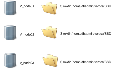
On each node in the cluster, create a directory where the node stores its data. For example:
$ mkdir /home/dbadmin/vertica/SSD
Vertica recommends that you create the same directory path on each node. Use this path when creating a storage location.
Use the CREATE LOCATION statement to add a storage location. Specify the following information:
-
The path on the node where Vertica stores the data.
Important
Vertica does not validate the path that you specify. Confirm that the path value points to a valid location.
-
The node where the location is available, or ALL NODES. If you specify ALL NODES, the statement creates the storage locations on all nodes in the cluster in a single transaction.
-
The type of information to be stored.
To give unprivileged (non-dbadmin) Linux users access to data, you must create a USER storage location. You can also use a USER storage location to give users without their own credentials access to shared file systems and object stores like HDFS and S3. See Creating a Storage Location for USER Access.
The following example shows how to add a location available on all nodes to store only data:
=> CREATE LOCATION '/home/dbadmin/vertica/SSD/' ALL NODES USAGE 'DATA';
The following example shows how to add a location that is available on the v_vmart_node0001 node to store data and temporary files:
=> CREATE LOCATION '/home/dbadmin/vertica/SSD/' NODE 'v_vmart_node0001';
Suppose you are using a storage location for data files and want to create ranked storage locations. In this ranking, columns are stored on different disks based on their measured performance. To create ranked storage locations, see Measuring storage performance and Setting storage performance.
After you create a storage location, you can alter the type of information it stores, with some restrictions. See Altering location use.
Storage location subdirectories
You cannot create a storage location in a subdirectory of an existing storage location. Doing so results in an error similar to the following:
=> CREATE LOCATION '/tmp/myloc' ALL NODES USAGE 'TEMP';
CREATE LOCATION
=> CREATE LOCATION '/tmp/myloc/ssd' ALL NODES USAGE 'TEMP';
ERROR 5615: Location [/tmp/myloc/ssd] conflicts with existing location
[/tmp/myloc] on node v_vmart_node0001
Creating labeled storage locations
You can add a storage location with a descriptive label using the CREATE LOCATION statement's LABEL keyword. You use labeled locations to set up storage policies. See Creating storage policies.
This example shows how to create a storage location on v_mart_node0002 with the label SSD:
=> CREATE LOCATION '/home/dbadmin/SSD/schemas' NODE 'v_vmart_node0002'
USAGE 'DATA' LABEL 'SSD';
This example shows you how to create a storage location on all nodes. Specifying the ALL NODES keyword adds the storage location to all nodes in a single transaction:
=> CREATE LOCATION '/home/dbadmin/SSD/schemas' ALL NODES
USAGE 'DATA' LABEL 'SSD';
The new storage location is listed in the DISK_STORAGE system table:
=> SELECT * FROM v_monitor.disk_storage;
.
.
-[ RECORD 7 ]-----------+-----------------------------------------------------
node_name | v_vmart_node0002
storage_path | /home/dbadmin/SSD/schemas
storage_usage | DATA
rank | 0
throughput | 0
latency | 0
storage_status | Active
disk_block_size_bytes | 4096
disk_space_used_blocks | 1549437
disk_space_used_mb | 6053
disk_space_free_blocks | 13380004
disk_space_free_mb | 52265
disk_space_free_percent | 89%
...
Creating a storage location for USER access
To give unprivileged (non-dbadmin) Linux users access to data, you must create a USER storage location.
By default, Vertica uses user-provided credentials to access external file systems such as HDFS and cloud object stores. You can override this default and create a USER storage location to manage access to these locations. To override the default, set the UseServerIdentityOverUserIdentity configuration parameter.
After you create a USER storage location, you can grant one or more users access to it. USER storage locations grant access only to data files, not temp files. You cannot assign a USER storage location to a storage policy. You cannot change an existing storage location to have USER access.
The following example shows how to create a USER storage location on a specific node:
=> CREATE LOCATION '/home/dbadmin/UserStorage/BobStore' NODE
'v_mcdb_node0007' USAGE 'USER';
The following example shows how to grant a specific user read and write permissions to the location:
=> GRANT ALL ON LOCATION '/home/dbadmin/UserStorage/BobStore' TO Bob;
GRANT PRIVILEGE
The following example shows how to use a USER storage location to grant access to locations on S3. Vertica uses the server credential to access the location:
--- set database-level credential (once):
=> ALTER DATABASE DEFAULT SET AWSAuth = 'myaccesskeyid123456:mysecretaccesskey123456789012345678901234';
=> CREATE LOCATION 's3://datalake' SHARED USAGE 'USER' LABEL 's3user';
=> CREATE ROLE ExtUsers;
--- Assign users to this role using GRANT (Role).
=> GRANT READ ON LOCATION 's3://datalake' TO ExtUsers;
For more information about configuring user privileges, see Database users and privileges and the GRANT (storage location) and REVOKE (storage location) reference pages.
Shared versus local storage
The SHARED keyword indicates that the location is shared by all nodes. Most remote file systems such as HDFS and S3 are shared. For these file systems, the path argument represents a single location in the remote file system where all nodes store data. Each node creates its own subdirectory in the shared storage location for its own files. Doing so prevents one node from overwriting files that belong to other nodes.
If using a remote file system, you must specify SHARED, even for one-node clusters. If the location is declared as USER, Vertica does not create subdirectories for each node. The setting of USER takes precedence over SHARED.
If you create a location and omit this keyword, the new storage location is treated as local. Each node must have unique access to the specified path. This location is usually a path in the node's own file system. Storage locations in file systems that are local to each node, such as Linux, are always local.
Deprecated
SHARED DATA storage locations are deprecated.
S3 storage of temporary data in Eon Mode
If you are using Vertica in Eon Mode and have limited local disk space, that space might be insufficient to handle the large quantities of temporary data that some DML operations can generate. This is especially true for large load operations and refresh operations.
You can leverage S3 storage to handle temporary data, as follows:
-
Create a remote storage location with CREATE LOCATION, where path is set to S3 as follows:
=> CREATE LOCATION 's3://bucket/path' ALL NODES SHARED USAGE 'TEMP';
-
Set the RemoteStorageForTemp session configuration parameter to 1:
=> ALTER SESSION SET RemoteStorageForTemp= 1;
A temporary storage location must already exist on S3 before you set this parameter to 1; otherwise, Vertica throws an error and hint to create the storage location.
-
Run the queries that require extra temporary storage.
-
Reset RemoteStorageForTemp to its default value:
=> ALTER SESSION DEFAULT CLEAR RemoteStorageForTemp;
When you set RemoteStorageForTemp, Vertica redirects temporary data for all DML operations to the specified remote location. The parameter setting remains in effect until it is explicitly reset to its default value (0), or the current session ends.
Important
Redirecting temporary data to S3 is liable to affect performance and require extra S3 API calls. Use it only for DML operations that involve large quantities of data.
16.3 - Storage locations on HDFS
You can place storage locations in HDFS, in addition to on the local Linux file system.
You can place storage locations in HDFS, in addition to on the local Linux file system. Because HDFS storage locations are not local, querying them can be slower. You might use HDFS storage locations for lower-priority data or data that is rarely queried (cold data). Moving lower-priority data to HDFS frees space on your Vertica cluster for higher-priority data.
If you are using Vertica for SQL on Apache Hadoop, you typically place storage locations only on HDFS.
16.3.1 - Requirements for HDFS storage locations
Caution
If you use HDFS storage locations, the HDFS data must be available when you start Vertica. Your HDFS cluster must be operational, and the ROS files must be present. If you moved data files, or they are corrupted, or your HDFS cluster is not responsive, Vertica cannot start.
To store Vertica's data on HDFS, verify that:
-
Your Hadoop cluster has WebHDFS enabled.
-
All of the nodes in your Vertica cluster can connect to all of the nodes in your Hadoop cluster. Any firewall between the two clusters must allow connections on the ports used by HDFS.
-
If your HDFS cluster is unsecured, you have a Hadoop user whose username matches the name of the Vertica database superuser (usually named dbadmin). This Hadoop user must have read and write access to the HDFS directory where you want Vertica to store its data.
-
If your HDFS cluster uses Kerberos authentication:
-
You have a Kerberos principal for Vertica, and it has read and write access to the HDFS directory that will be used for the storage location. See Kerberos below for instructions.
-
The Kerberos KDC is running.
-
Your HDFS cluster has enough storage available for Vertica data. See Space Requirements below for details.
-
The data you store in an HDFS-backed storage location does not expand your database's size beyond any data allowance in your Vertica license. Vertica counts data stored in an HDFS-backed storage location as part of any data allowance set by your license. See Managing licenses in the Administrator's Guide for more information.
Backup/Restore has additional requirements.
Space requirements
If your Vertica database is K-safe, HDFS-based storage locations contain two copies of the data you store in them. One copy is the primary projection, and the other is the buddy projection. If you have enabled HDFS's data-redundancy feature, Hadoop stores both projections multiple times. This duplication might seem excessive. However, it is similar to how a RAID level 1 or higher stores redundant copies of both the primary and buddy projections. The redundant copies also help the performance of HDFS by enabling multiple nodes to process a request for a file.
Verify that your HDFS installation has sufficient space available for redundant storage of both the primary and buddy projections of your K-safe data. You can adjust the number of duplicates stored by HDFS by setting the HadoopFSReplication configuration parameter. See Troubleshooting HDFS Storage Locations for details.
Kerberos
To use a storage location in HDFS with Kerberos, take the following additional steps:
-
Create a Kerberos principal for each Vertica node as explained in Using Kerberos with Vertica.
-
Give all node principals read and write permission to the HDFS directory you will use as a storage location.
If you plan to use vbr to back up and restore the location, see additional requirements in Requirements for backing up and restoring HDFS storage locations.
Adding HDFS storage locations to new nodes
If you add nodes to your Vertica cluster, they do not automatically have access to existing HDFS storage locations. You must manually create the storage location for the new node using the CREATE LOCATION statement. Do not use the ALL NODES option in this statement. Instead, use the NODE option with the name of the new node to tell Vertica that just that node needs to add the shared location.
Caution
You must manually create the storage location. Otherwise, the new node uses the default storage policy (usually, storage on the local Linux file system) to store data that the other nodes store in HDFS. As a result, the node can run out of disk space.
Consider an HDFS storage location that was created on a three-node cluster with the following statements:
=> CREATE LOCATION 'hdfs://hadoopNS/vertica/colddata' ALL NODES SHARED
USAGE 'data' LABEL 'coldstorage';
=> SELECT SET_OBJECT_STORAGE_POLICY('SchemaName','coldstorage');
The following example shows how to add the storage location to a new cluster node:
=> CREATE LOCATION 'hdfs://hadoopNS/vertica/colddata' NODE 'v_vmart_node0004'
SHARED USAGE 'data' LABEL 'coldstorage';
Any active standby nodes in your cluster when you create an HDFS storage location automatically create their own instances of the location. When the standby node takes over for a down node, it uses its own instance of the location to store data for objects using the HDFS storage policy. Treat standby nodes added after you create the storage location as any other new node. You must manually define the HDFS storage location.
16.3.2 - How the HDFS storage location stores data
Vertica stores data in storage locations on HDFS similarly to the way it stores data in the Linux file system.
Vertica stores data in storage locations on HDFS similarly to the way it stores data in the Linux file system. When you create a storage location on HDFS, Vertica stores the ROS containers holding its data on HDFS. You can choose which data uses the HDFS storage location: from the data for just a single table or partition to all of the database's data.
When Vertica reads data from or writes data to an HDFS storage location, the node storing or retrieving the data contacts the Hadoop cluster directly to transfer the data. If a single ROS container file is split among several HDFS nodes, the Vertica node connects to each of them. The Vertica node retrieves the pieces and reassembles the file. Because each node fetches its own data directly from the source, data transfers are parallel, increasing their efficiency. Having the Vertica nodes directly retrieve the file splits also reduces the impact on the Hadoop cluster.
What you can store in HDFS
Use HDFS storage locations to store only data. You cannot store catalog information in an HDFS storage location.
Caution
While it is possible to use an HDFS storage location for temporary data storage, you must never do so. Using HDFS for temporary storage causes severe performance issues.
What HDFS storage locations cannot do
Because Vertica uses storage locations to store ROS containers in a proprietary format, MapReduce and other Hadoop components cannot access your Vertica ROS data stored in HDFS. Never allow another program that has access to HDFS to write to the ROS files. Any outside modification of these files can lead to data corruption and loss. Applications must use the Vertica client libraries to access Vertica data. If you want to share ROS data with other Hadoop components, you can export it (see File export).
16.3.3 - Best practices for Vertica for SQL on Apache Hadoop
If you are using the Vertica for SQLxa0on Apache Hadoop product, Vertica recommends the following best practices for storage locations:.
If you are using the Vertica for SQL on Apache Hadoop product, Vertica recommends the following best practices for storage locations:
-
Place only data type storage locations on HDFS storage.
-
Place temp space directly on the local Linux file system, not in HDFS.
-
For the best performance, place the Vertica catalog directly on the local Linux file system.
-
Create the database first on a local Linux file system. Then, you can extend the database to HDFS storage locations and set storage policies that exclusively place data blocks on the HDFS storage location.
-
For better performance, if you are running Vertica only on a subset of the HDFS nodes, do not run the HDFS balancer on them. The HDFS balancer can move data blocks farther away, causing Vertica to read non-local data during query execution. Queries run faster if they do not require network I/O.
Generally, HDFS requires approximately 2 GB of memory for each node in the cluster. To support this requirement in your Vertica configuration:
-
Create a 2-GB resource pool.
-
Do not assign any Vertica execution resources to this pool. This approach reserves the space for use by HDFS.
Alternatively, use Ambari or Cloudera Manager to find the maximum heap size required by HDFS and set the size of the resource pool to that value.
For more about how to configure resource pools, see Managing workloads.
16.3.4 - Troubleshooting HDFS storage locations
This topic explains some common issues with HDFS storage locations.
This topic explains some common issues with HDFS storage locations.
HDFS storage disk consumption
By default, HDFS makes three copies of each file it stores. This replication helps prevent data loss due to disk or system failure. It also helps increase performance by allowing several nodes to handle a request for a file.
A Vertica database with a K-safety value of 1 or greater also stores its data redundantly using buddy projections.
When a K-Safe Vertica database stores data in an HDFS storage location, its data redundancy is compounded by HDFS's redundancy. HDFS stores three copies of the primary projection's data, plus three copies of the buddy projection for a total of six copies of the data.
If you want to reduce the amount of disk storage used by HDFS locations, you can alter the number of copies of data that HDFS stores. The Vertica configuration parameter named HadoopFSReplication controls the number of copies of data HDFS stores.
You can determine the current HDFS disk usage by logging into the Hadoop NameNode and issuing the command:
$ hdfs dfsadmin -report
This command prints the usage for the entire HDFS storage, followed by details for each node in the Hadoop cluster. The following example shows the beginning of the output from this command, with the total disk space highlighted:
$ hdfs dfsadmin -report
Configured Capacity: 51495516981 (47.96 GB)
Present Capacity: 32087212032 (29.88 GB)
DFS Remaining: 31565144064 (29.40 GB)
DFS Used: 522067968 (497.88 MB)
DFS Used%: 1.63%
Under replicated blocks: 0
Blocks with corrupt replicas: 0
Missing blocks: 0
. . .
After loading a simple million-row table into a table stored in an HDFS storage location, the report shows greater disk usage:
Configured Capacity: 51495516981 (47.96 GB)
Present Capacity: 32085299338 (29.88 GB)
DFS Remaining: 31373565952 (29.22 GB)
DFS Used: 711733386 (678.76 MB)
DFS Used%: 2.22%
Under replicated blocks: 0
Blocks with corrupt replicas: 0
Missing blocks: 0
. . .
The following Vertica example demonstrates:
-
Creating the storage location on HDFS.
-
Dropping the table in Vertica.
-
Setting the HadoopFSReplication configuration option to 1. This tells HDFS to store a single copy of an HDFS storage location's data.
-
Recreating the table and reloading its data.
=> CREATE LOCATION 'hdfs://hadoopNS/user/dbadmin' ALL NODES SHARED
USAGE 'data' LABEL 'hdfs';
CREATE LOCATION
=> DROP TABLE messages;
DROP TABLE
=> ALTER DATABASE DEFAULT SET PARAMETER HadoopFSReplication = 1;
=> CREATE TABLE messages (id INTEGER, text VARCHAR);
CREATE TABLE
=> SELECT SET_OBJECT_STORAGE_POLICY('messages', 'hdfs');
SET_OBJECT_STORAGE_POLICY
----------------------------
Object storage policy set.
(1 row)
=> COPY messages FROM '/home/dbadmin/messages.txt';
Rows Loaded
-------------
1000000
Running the HDFS report on Hadoop now shows less disk space use:
$ hdfs dfsadmin -report
Configured Capacity: 51495516981 (47.96 GB)
Present Capacity: 32086278190 (29.88 GB)
DFS Remaining: 31500988416 (29.34 GB)
DFS Used: 585289774 (558.18 MB)
DFS Used%: 1.82%
Under replicated blocks: 0
Blocks with corrupt replicas: 0
Missing blocks: 0
. . .
Caution
Reducing the number of copies of data stored by HDFS increases the risk of data loss. It can also negatively impact the performance of HDFS by reducing the number of nodes that can provide access to a file. This slower performance can impact the performance of Vertica queries that involve data stored in an HDFS storage location.
ERROR 6966: StorageBundleWriter
You might encounter Error 6966 when loading data into a storage location on a small Hadoop cluster (5 or fewer data nodes). This error is caused by the way HDFS manages the write pipeline and replication. You can mitigate this problem by reducing the number of replicas as explained in HDFS Storage Disk Consumption. For configuration changes you can make in the Hadoop cluster instead, see this blog post from Hortonworks.
Kerberos authentication when creating a storage location
If HDFS uses Kerberos authentication, then the CREATE LOCATION statement authenticates using the Vertica keytab principal, not the principal of the user performing the action. If the creation fails with an authentication error, verify that you have followed the steps described in Kerberos to configure this principal.
When creating an HDFS storage location on a Hadoop cluster using Kerberos, CREATE LOCATION reports the principal being used as in the following example:
=> CREATE LOCATION 'hdfs://hadoopNS/user/dbadmin' ALL NODES SHARED
USAGE 'data' LABEL 'coldstorage';
NOTICE 0: Performing HDFS operations using kerberos principal [vertica/hadoop.example.com]
CREATE LOCATION
Backup or restore fails
For issues with backup/restore of HDFS storage locations, see Troubleshooting backup and restore.
16.4 - Altering location use
ALTER_LOCATION_USE lets you change the type of files that Vertica stores at a storage location.
ALTER_LOCATION_USE lets you change the type of files that Vertica stores at a storage location. You typically use labels only for DATA storage locations, not TEMP.
This example shows how to alter the storage location on v_vmartdb_node0004 to store only data files:
=> SELECT ALTER_LOCATION_USE ('/thirdVerticaStorageLocation/' , 'v_vmartdb_node0004' , 'DATA');
Altering HDFS storage locations
When altering an HDFS storage location, you must make the change for all nodes in the Vertica cluster. To do so, specify a node value of '', as in the following example:
=> SELECT ALTER_LOCATION_USE('hdfs:///user/dbadmin/v_vmart',
'','TEMP');
Restrictions
You cannot change a storage location from a USER usage type if you created the location that way, or to a USER type if you did not. You can change a USER storage location to specify DATA (storing TEMP files is not supported). However, doing so does not affect the primary objective of a USER storage location, to be accessible by non-dbadmin users with assigned privileges.
You cannot change a storage location from SHARED TEMP or SHARED USER to SHARED DATA or the reverse.
Effects of altering storage location use
Before altering a storage location use type, be aware that at least one location must remain for storing data and temp files on a node. You can store data and temp files in the same, or separate, storage locations.
Altering an existing storage location has the following effects:
|
Alter use from... |
To store only... |
Has this effect... |
|
Temp and data files (or data only) |
Temp files |
Data content is eventually merged out by the Tuple Mover.You can also manually merge out data from the storage location using DO_TM_TASK.
The location stores only temp files from that point forward.
|
|
Temp and data files (or temp only) |
Data files |
Vertica continues to run all statements that use temp files (such as queries and loads).
Subsequent statements no longer use the changed storage location for temp files, and the location stores only data files from that point forward.
|
16.5 - Altering location labels
ALTER_LOCATION_LABEL lets you change the label for a storage location in several ways:.
ALTER_LOCATION_LABEL lets you change the label for a storage location in several ways:
You can perform these operations on individual nodes or cluster-wide.
Adding a location label
You add a location label to an unlabeled storage location with ALTER_LOCATION_LABEL. For example, unlabeled storage location /home/dbadmin/Vertica/SSD is defined on a three-node cluster:
You can label this storage location as SSD on all nodes as follows:
=> SELECT ALTER_LOCATION_LABEL('/home/dbadmin/vertica/SSD', '', 'SSD');
Caution
If you label a storage location that contains data, Vertica moves the data to an unlabeled location, if one exists. To prevent data movement between storage locations, labels should be applied either to all storage locations or none.
Removing a location label
You can remove a location label only if the following conditions are both true:
The following statement removes the SSD label from the specified storage location on all nodes:
=> SELECT ALTER_LOCATION_LABEL('/home/dbadmin/SSD/tables','', '');
ALTER_LOCATION_LABEL
------------------------------------------
/home/dbadmin/SSD/tables label changed.
(1 row)
Altering a storage location label
You can relabel a storage location only if no database object has a storage policy that specifies this label.
16.6 - Creating storage policies
Vertica meta-function SET_OBJECT_STORAGE_POLICY creates a that associates a database object with a labeled storage location.
Vertica meta-function
SET_OBJECT_STORAGE_POLICY creates a storage policy that associates a database object with a labeled storage location. When an object has a storage policy, Vertica uses the labeled location as the default storage location for that object's data.
You can create storage policies for the database, schemas, tables, and partition ranges. Each object can be associated with one storage policy. Each time data is loaded and updated, Vertica checks whether the object has a storage policy. If it does, Vertica uses the labeled storage location. If no storage policy exists for an object or its parent entities, data storage processing continues using standard storage algorithms on available storage locations. If all storage locations are labeled, Vertica uses one of them.
Storage policies let you determine where to store critical data. For example, you might create a storage location with the label SSD that represents the fastest available storage on the cluster nodes. You then create storage policies to associate tables with that labeled location. For example, the following SET_OBJECT_STORAGE_POLICY statement sets a storage policy on table test to use the storage location labeled SSD as its default location:
=> SELECT SET_OBJECT_STORAGE_POLICY('test','ssd', true);
SET_OBJECT_STORAGE_POLICY
--------------------------------------------------
Object storage policy set.
Task: moving storages
(Table: public.test) (Projection: public.test_b0)
(Table: public.test) (Projection: public.test_b1)
(1 row)
Note
You cannot include temporary files in storage policies. Storage policies are for use only with data files on storage locations for DATA. Storage policies are not valid for USER locations.
Creating one or more storage policies does not require that policies exist for all database objects. A site can support objects with or without storage policies. You can add storage policies for a discrete set of priority objects, while letting other objects exist without a policy, so they use available storage.
You can measure the performance of any disk storage location (see Measuring storage performance). Then, using the performance measurements, set the storage location performance. Vertica uses the performance measurements you set to rank its storage locations and, through ranking, to determine which key projection columns to store on higher performing locations, as described in Setting storage performance.
If you already set the performance of your site's storage locations, and decide to use storage policies, any storage location with an associated policy has a higher priority than the storage ranking setting.
You can use storage policies to move older data to less-expensive storage locations while keeping it available for queries. See Creating storage policies for low-priority data.
Storage hierarchy and precedence
Vertica determines where to store object data according to the following hierarchy of storage policies, listed below in ascending order of precedence:
-
Database
-
Schema
-
Table
-
Table partition
If an object lacks its own storage policy, it uses the storage policy of its parent object. For example, table Region.Income in database Sales is partitioned by months. Labeled storage policies FAST and STANDARD are assigned to the table and database, respectively. No storage policy is assigned to the table's partitions or its parent schema, so these use the storage policies of their parent objects, FAST and STANDARD, respectively:
|
Object |
Storage policy |
Policy precedence |
Labeled location |
Default location |
Sales (database) |
YES |
4 |
STANDARD |
STANDARD |
Region (schema) |
NO |
3 |
N/A |
STANDARD |
Income (table) |
YES |
2 |
FAST |
FAST |
MONTH (partitions) |
NO |
1 |
N/A |
FAST |
When Tuple Mover operations such as mergeout occur, all Income data moves to the FAST storage location. Other tables in the Region schema use their own storage policy. If a Region table lacks its own storarage policy, Tuple Mover uses the next storage policy above it—in this case, it uses database storage policy and moves the table data to STANDARD.
Querying existing storage policies
You can query existing storage policies, listed in the location_label column of system table STORAGE_CONTAINERS:
=> SELECT node_name, projection_name, location_label FROM v_monitor.storage_containers;
node_name | projection_name | location_label
------------------+----------------------+----------------
v_vmart_node0001 | states_p |
v_vmart_node0001 | states_p |
v_vmart_node0001 | t1_b1 |
v_vmart_node0001 | newstates_b0 | LEVEL3
v_vmart_node0001 | newstates_b0 | LEVEL3
v_vmart_node0001 | newstates_b1 | LEVEL3
v_vmart_node0001 | newstates_b1 | LEVEL3
v_vmart_node0001 | newstates_b1 | LEVEL3
v_vmart_node0001 | states_p_v1_node0001 | LEVEL3
v_vmart_node0001 | states_p_v1_node0001 | LEVEL3
v_vmart_node0001 | states_p_v1_node0001 | LEVEL3
v_vmart_node0001 | states_p_v1_node0001 | LEVEL3
v_vmart_node0001 | states_p_v1_node0001 | LEVEL3
v_vmart_node0001 | states_p_v1_node0001 | LEVEL3
v_vmart_node0001 | states_b0 | SSD
v_vmart_node0001 | states_b0 | SSD
v_vmart_node0001 | states_b1 | SSD
v_vmart_node0001 | states_b1 | SSD
v_vmart_node0001 | states_b1 | SSD
...
Forcing existing data storage to a new storage location
By default, the Tuple Mover enforces object storage policies after all pending mergeout operations are complete. SET_OBJECT_STORAGE_POLICY moves existing data storage to a new location immediately, if you set its parameter enforce‑storage‑move to true. You might want to force a move, even though it means waiting for the operation to complete before continuing, if the data being moved is old. The Tuple Mover runs less frequently on older data.
Note
If parameter enforce‑storage‑move is set to true, SET_OBJECT_STORAGE_POLICY performs a cluster-wide operation. If an error occurs on any node, the function displays a warning message and skips that node. It then continues executing the operation on the remaining nodes.
16.7 - Creating storage policies for low-priority data
If some of your data is in a partitioned table, you can move less-queried partitions to less-expensive storage such as HDFS.
If some of your data is in a partitioned table, you can move less-queried partitions to less-expensive storage such as HDFS. The data is still accessible in queries, just at a slower speed. In this scenario, the faster storage is often referred to as "hot storage," and the slower storage is referred to as "cold storage."
Suppose you have a table named messages (containing social-media messages) that is partitioned by the year and month of the message's timestamp. You can list the partitions in the table by querying the PARTITIONS system table.
=> SELECT partition_key, projection_name, node_name, location_label FROM partitions
ORDER BY partition_key;
partition_key | projection_name | node_name | location_label
--------------+-----------------+------------------+----------------
201309 | messages_b1 | v_vmart_node0001 |
201309 | messages_b0 | v_vmart_node0003 |
201309 | messages_b1 | v_vmart_node0002 |
201309 | messages_b1 | v_vmart_node0003 |
201309 | messages_b0 | v_vmart_node0001 |
201309 | messages_b0 | v_vmart_node0002 |
201310 | messages_b0 | v_vmart_node0002 |
201310 | messages_b1 | v_vmart_node0003 |
201310 | messages_b0 | v_vmart_node0001 |
. . .
201405 | messages_b0 | v_vmart_node0002 |
201405 | messages_b1 | v_vmart_node0003 |
201405 | messages_b1 | v_vmart_node0001 |
201405 | messages_b0 | v_vmart_node0001 |
(54 rows)
Next, suppose you find that most queries on this table access only the latest month or two of data. You might decide to move the older data to cold storage in an HDFS-based storage location. After you move the data, it is still available for queries, but with lower query performance.
To move partitions to the HDFS storage location, supply the lowest and highest partition key values to be moved in the SET_OBJECT_STORAGE_POLICY function call. The following example shows how to move data between two dates. In this example:
-
The partition key value 201309 represents September 2013.
-
The partition key value 201403 represents March 2014.
-
The name, coldstorage, is the label of the HDFS-based storage location.
-
The final argument, which is optional, is true, meaning that the function does not return until the move is complete. By default the function returns immediately and the data is moved when the Tuple Mover next runs. When data is old, however, the Tuple Mover runs less frequently, which would delay recovering the original storage space.
=> SELECT SET_OBJECT_STORAGE_POLICY('messages','coldstorage', '201309', '201403', 'true');
The partitions within the specified range are moved to the HDFS storage location labeled coldstorage the next time the Tuple Mover runs. This location name now displays in the PARTITIONS system table's location_label column.
=> SELECT partition_key, projection_name, node_name, location_label
FROM partitions ORDER BY partition_key;
partition_key | projection_name | node_name | location_label
--------------+-----------------+------------------+----------------
201309 | messages_b0 | v_vmart_node0003 | coldstorage
201309 | messages_b1 | v_vmart_node0001 | coldstorage
201309 | messages_b1 | v_vmart_node0002 | coldstorage
201309 | messages_b0 | v_vmart_node0001 | coldstorage
. . .
201403 | messages_b0 | v_vmart_node0002 | coldstorage
201404 | messages_b0 | v_vmart_node0001 |
201404 | messages_b0 | v_vmart_node0002 |
201404 | messages_b1 | v_vmart_node0001 |
201404 | messages_b1 | v_vmart_node0002 |
201404 | messages_b0 | v_vmart_node0003 |
201404 | messages_b1 | v_vmart_node0003 |
201405 | messages_b0 | v_vmart_node0001 |
201405 | messages_b1 | v_vmart_node0002 |
201405 | messages_b0 | v_vmart_node0002 |
201405 | messages_b0 | v_vmart_node0003 |
201405 | messages_b1 | v_vmart_node0001 |
201405 | messages_b1 | v_vmart_node0003 |
(54 rows)
After your initial data move, you can move additional data to the HDFS storage location periodically. You can move individual partitions or a range of partitions from the "hot" storage to the "cold" storage location using the same method:
=> SELECT SET_OBJECT_STORAGE_POLICY('messages', 'coldstorage', '201404', '201404', 'true');
=> SELECT projection_name, node_name, location_label
FROM PARTITIONS WHERE PARTITION_KEY = '201404';
projection_name | node_name | location_label
-----------------+------------------+----------------
messages_b0 | v_vmart_node0002 | coldstorage
messages_b0 | v_vmart_node0003 | coldstorage
messages_b1 | v_vmart_node0003 | coldstorage
messages_b0 | v_vmart_node0001 | coldstorage
messages_b1 | v_vmart_node0002 | coldstorage
messages_b1 | v_vmart_node0001 | coldstorage
(6 rows)
Moving partitions to a table stored on HDFS
Another method of moving partitions from hot storage to cold storage is to move the partitions' data to a separate table in the other storage location. This method breaks the data into two tables, one containing hot data and the other containing cold data. Use this method if you want to prevent queries from inadvertently accessing data stored in cold storage. To query the older data, you must explicitly query the cold table.
To move partitions:
-
Create a new table whose schema matches that of the existing partitioned table.
-
Set the storage policy of the new table to use the HDFS-based storage location.
-
Use the MOVE_PARTITIONS_TO_TABLE function to move a range of partitions from the hot table to the cold table. The partitions migrate when the Tuple Mover next runs.
The following example demonstrates these steps. You first create a table named cold_messages. You then assign it the HDFS-based storage location named coldstorage, and, finally, move a range of partitions.
=> CREATE TABLE cold_messages LIKE messages INCLUDING PROJECTIONS;
=> SELECT SET_OBJECT_STORAGE_POLICY('cold_messages', 'coldstorage');
=> SELECT MOVE_PARTITIONS_TO_TABLE('messages','201309','201403','cold_messages');
16.8 - Moving data storage locations
SET_OBJECT_STORAGE_POLICY moves data storage from an existing location (labeled and unlabeled) to another labeled location.
SET_OBJECT_STORAGE_POLICY moves data storage from an existing location (labeled and unlabeled) to another labeled location. This function performs two tasks:
-
Creates a storage policy for an object, or changes its current policy.
-
Moves all existing data for the specified objects to the target storage location.
Before it moves object data to the specified storage location, Vertica calculates the required storage and checks available space at the target. Before calling SET_OBJECT_STORAGE_POLICY, check available space on the new target location. Be aware that checking does not guarantee that this space remains available when the Tuple Mover actually executes the move. If the storage location lacks sufficient free space, the function returns an error.
Note
Moving an object's current storage to a new target is a cluster-wide operation. If a node is unavailable, the function returns a warning message, and then continues to implement the move on other nodes. When the node rejoins the cluster, the Tuple Mover updates it with the storage data.
By default, the Tuple Mover moves object data to the new storage location after all pending mergeout tasks return. You can force the data to move immediately by setting the function's enforce-storage-move argument to true. For example, the following statement sets the storage policy for a table and implements the move immediately:
=> SELECT SET_OBJECT_STORAGE_POLICY('states', 'SSD', 'true');
SET_OBJECT_STORAGE_POLICY
------------------------------------------------------------------------------------------------
Object storage policy set.
Task: moving storages
(Table: public.states) (Projection: public.states_p1)
(Table: public.states) (Projection: public.states_p2)
(Table: public.states) (Projection: public.states_p3)
(1 row)
Tip
Consider using the
ENFORCE_OBJECT_STORAGE_POLICY meta-function to relocate the data of multiple database objects as needed, to bring them into compliance with current storage policies. Using this function is equivalent to calling
SET_OBJECT_STORAGE_POLICY successively on multiple database objects and setting the
enforce-storage-move argument to true.
16.9 - Clearing storage policies
The CLEAR_OBJECT_STORAGE_POLICY meta-function clears a storage policy from a database, schema, table, or table partition.
The CLEAR_OBJECT_STORAGE_POLICY meta-function clears a storage policy from a database, schema, table, or table partition. For example, the following statement clears the storage policy for a table:
=> SELECT CLEAR_OBJECT_STORAGE_POLICY ('store.store_sales_fact');
CLEAR_OBJECT_STORAGE_POLICY
--------------------------------
Object storage policy cleared.
(1 row)
The Tuple Mover moves existing storage containers to the parent storage policy's location, or the default storage location if there is no parent policy. By default, this move occurs after all pending mergeout tasks return.
You can force the data to move immediately by setting the function's enforce-storage-move argument to true. For example, the following statement clears the storage policy for a table and implements the move immediately:
=> SELECT CLEAR_OBJECT_STORAGE_POLICY ('store.store_orders_fact', 'true');
CLEAR_OBJECT_STORAGE_POLICY
-----------------------------------------------------------------------------
Object storage policy cleared.
Task: moving storages
(Table: store.store_orders_fact) (Projection: store.store_orders_fact_b0)
(Table: store.store_orders_fact) (Projection: store.store_orders_fact_b1)
(1 row)
Tip
Consider using the
ENFORCE_OBJECT_STORAGE_POLICY meta-function to relocate the data of multiple database objects as needed, to bring them into compliance with current storage policies. Using this function is equivalent to calling
CLEAR_OBJECT_STORAGE_POLICY successively on multiple database objects and setting
enforce-storage-move to true.
Clearing a storage policy at one level, such as a table, does not necessarily affect storage policies at other levels, such as that table's partitions.
For example, the lineorder table has a storage policy to store table data at a location labeled F2. Various partitions in this table are individually assigned their own storage locations, as verified by querying the STORAGE_POLICIES system table:
=> SELECT * from v_monitor.storage_policies;
schema_name | object_name | policy_details | location_label
-------------+-------------+------------------+----------------
| public | Schema | F4
public | lineorder | Partition [0, 0] | F1
public | lineorder | Partition [1, 1] | F2
public | lineorder | Partition [2, 2] | F4
public | lineorder | Partition [3, 3] | M1
public | lineorder | Partition [4, 4] | M3
(6 rows)
Clearing the current storage policy from the lineorder table has no effect on the storage policies of its individual partitions. For example, given the following CLEAR_OBJECT_STORAGE_POLICY statement:
=> SELECT CLEAR_OBJECT_STORAGE_POLICY ('lineorder');
CLEAR_OBJECT_STORAGE_POLICY
-------------------------------------
Default storage policy cleared.
(1 row)
The individual partitions in the table retain their storage policies:
=> SELECT * from v_monitor.storage_policies;
schema_name | object_name | policy_details | location_label
-------------+-------------+------------------+----------------
| public | Schema | F4
public | lineorder | Partition [0, 0] | F1
public | lineorder | Partition [1, 1] | F2
public | lineorder | Partition [2, 2] | F4
public | lineorder | Partition [3, 3] | M1
public | lineorder | Partition [4, 4] | M3
(6 rows)
If you clear storage policies from a range of partitions key in a table, the storage policies of parent objects and other partition ranges are unaffected. For example, the following statement clears storage policies from partition keys 0 through 3:
=> SELECT CLEAR_OBJECT_STORAGE_POLICY ('lineorder','0','3');
clear_object_storage_policy
-------------------------------------
Default storage policy cleared.
(1 row)
=> SELECT * from storage_policies;
schema_name | object_name | policy_details | location_label
-------------+-------------+------------------+----------------
| public | Schema | F4
public | lineorder | Table | F2
public | lineorder | Partition [4, 4] | M3
(2 rows)
16.10 - Measuring storage performance
Vertica lets you measure disk I/O performance on any storage location at your site.
Vertica lets you measure disk I/O performance on any storage location at your site. You can use the returned measurements to set performance, which automatically provides rank. Depending on your storage needs, you can also use performance to determine the storage locations needed for critical data as part of your site's storage policies. Storage performance measurements apply only to data storage locations, not temporary storage locations.
Measuring storage location performance calculates the time it takes to read and write 1 MB of data from the disk, which equates to:
IO time = time to read/write 1MB + time to seek = 1/throughput + 1/Latency
Thus, the I/O time of a faster storage location is less than that of a slower storage location.
Note
Measuring storage location performance requires extensive disk I/O, which is a resource-intensive operation. Consider starting this operation when fewer other operations are running.
Vertica gives you two ways to measure storage location performance, depending on whether the database is running. You can either:
Both methods return the throughput and latency for the storage location. Record or capture the throughput and latency information so you can use it to set the location performance (see Setting storage performance).
Use the MEASURE_LOCATION_PERFORMANCE() function to measure performance for a storage location when the database is running. This function has the following requirements:
-
The storage path must already exist in the database.
-
You need RAM*2 free space available in a storage location to measure its performance. For example, if you have 16 GB RAM, you need 32 GB of available disk space. If you do not have enough disk space, the function returns an error.
Use the system table DISK_STORAGE to obtain information about disk storage on each database node.
The following example shows how to measure the performance of a storage location on v_vmartdb_node0004:
=> SELECT MEASURE_LOCATION_PERFORMANCE('/secondVerticaStorageLocation/','v_vmartdb_node0004');
WARNING: measure_location_performance can take a long time. Please check logs for progress
measure_location_performance
--------------------------------------------------
Throughput : 122 MB/sec. Latency : 140 seeks/sec
You can measure disk performance before setting up a cluster. This approach is useful when you want to verify that the disk is functioning within normal parameters. To perform this measurement, you must already have Vertica installed.
To measure disk performance, use the following command:
opt/vertica/bin/vertica -m <path to disk mount>
For example:
opt/vertica/bin/vertica -m /secondVerticaStorageLocation/node0004_data
16.11 - Setting storage performance
You can use the measurements returned from the MEASURE_LOCATION_PERFORMANCE function as input values to the SET_LOCATION_PERFORMANCE() function.
You can use the measurements returned from the MEASURE_LOCATION_PERFORMANCE function as input values to the SET_LOCATION_PERFORMANCE() function.
Note
You must set the throughput and latency parameters of this function to 1 or more.
The following example shows how to set the performance of a storage location on v_vmartdb_node0004, using values for this location returned from the MEASURE_LOCATION_PERFORMANCE function. Set the throughput to 122 MB/second and the latency to 140 seeks/second. MEASURE_LOCATION_PERFORMANCE
=> SELECT SET_LOCATION_PERFORMANCE('/secondVerticaStorageLocation/','node2','122','140');
After you set performance-data parameters, Vertica automatically uses performance data to rank storage locations whenever it stores projection columns.
Vertica stores columns included in the projection sort order on the fastest available storage locations. Columns not included in the projection sort order are stored on slower disks. Columns for each projection are ranked as follows:
-
Columns in the sort order are given the highest priority (numbers > 1000).
-
The last column in the sort order is given the rank number 1001.
-
The next-to-last column in the sort order is given the rank number 1002, and so on until the first column in the sort order is given 1000 + # of sort columns.
-
The remaining columns are given numbers from 1000–1, starting with 1000 and decrementing by one per column.
Vertica then stores columns on disk from the highest ranking to the lowest ranking. It places highest-ranking columns on the fastest disks and the lowest-ranking columns on the slowest disks.
You initially measure location performance and set it in the Vertica database. Then, you can use the performance results to determine the fastest storage to use in your storage policies.
-
Set the locations with the highest performance as the default locations for critical data.
-
Use slower locations as default locations for older, or less-important data. Such slower locations may not require policies at all, if you do not want to specify default locations.
Vertica determines data storage as follows, depending on whether a storage policy exists:
|
Storage policy |
Label |
# Locations |
Vertica action |
|
No |
No |
Multiple |
Uses ranking (as described), choosing a location from all locations that exist. |
|
Yes |
Yes |
Single |
Uses that storage location exclusively. |
|
Yes |
Yes |
Multiple |
Ranks storage (as described) among all same-name labeled locations. |
16.12 - Retiring storage locations
You can retire a storage location to stop using it.
You can retire a storage location to stop using it. Retiring a storage location prevents Vertica from storing data or temp files to it, but does not remove the actual location. Any data previously stored on the retired location is eventually merged out by the Tuple Mover. Use the RETIRE_LOCATION function to retire a location.
The following example retires a location from a single node:
=> SELECT RETIRE_LOCATION('/secondStorageLocation/' , 'v_vmartdb_node0004');
To retire a storage location on all nodes, use an empty string ('') for the second argument. If the location is SHARED, you can retire it only on all nodes.
You can expedite retiring and then dropping a storage location by passing an optional third argument, enforce, as true. With this directive, the function moves the data out of the storage location instead of waiting for the Tuple Mover, allowing you to drop the location immediately.
You can also use the ENFORCE_OBJECT_STORAGE_POLICY function to trigger the move for all storage locations at once, which allows you to drop the locations. This approach is equivalent to using the enforce argument.
The following example shows how to retire a storage location on all nodes so that it can be immediately dropped:
=> SELECT RETIRE_LOCATION('/secondStorageLocation/' , '', true);
Note
If the location used in a storage policy is the last available storage for its associated objects, you cannot retire it unless you set enforce to true.
Data and temp files can be stored in one, or multiple separate, storage locations.
For further information on dropping a location after retiring it, see Dropping storage locations.
16.13 - Restoring retired storage locations
You can restore a previously retired storage location.
You can restore a previously retired storage location. After the location is restored, Vertica re-ranks the storage location and uses the restored location to process queries as determined by its rank.
Use the RESTORE_LOCATION function to restore a retired storage location.
The following example shows how to restore a retired storage location on a single node:
=> SELECT RESTORE_LOCATION('/secondStorageLocation/' , 'v_vmartdb_node0004');
To restore a storage location on all nodes, use an empty string ('') for the second argument. The following example demonstrates creating, retiring, and restoring a location on all nodes:
=> CREATE LOCATION '/tmp/ab1' ALL NODES USAGE 'TEMP';
CREATE LOCATION
=> SELECT RETIRE_LOCATION('/tmp/ab1', '');
retire_location
------------------------
/tmp/ab1 retired.
(1 row)
=> SELECT location_id, node_name, location_path, location_usage, is_retired
FROM STORAGE_LOCATIONS WHERE location_path ILIKE '/tmp/ab1';
location_id | node_name | location_path | location_usage | is_retired
------------------+---------------------+---------------+----------------+------------
45035996273736724 | v_vmart_node0001 | /tmp/ab1 | TEMP | t
45035996273736726 | v_vmart_node0002 | /tmp/ab1 | TEMP | t
45035996273736728 | v_vmart_node0003 | /tmp/ab1 | TEMP | t
45035996273736730 | v_vmart_node0004 | /tmp/ab1 | TEMP | t
(4 rows)
=> SELECT RESTORE_LOCATION('/tmp/ab1', '');
restore_location
-------------------------
/tmp/ab1 restored.
(1 row)
=> SELECT location_id, node_name, location_path, location_usage, is_retired
FROM STORAGE_LOCATIONS WHERE location_path ILIKE '/tmp/ab1';
location_id | node_name | location_path | location_usage | is_retired
------------------+---------------------+---------------+----------------+------------
45035996273736724 | v_vmart_node0001 | /tmp/ab1 | TEMP | f
45035996273736726 | v_vmart_node0002 | /tmp/ab1 | TEMP | f
45035996273736728 | v_vmart_node0003 | /tmp/ab1 | TEMP | f
45035996273736730 | v_vmart_node0004 | /tmp/ab1 | TEMP | f
(4 rows)
RESTORE_LOCATION restores the location only on the nodes where the location exists and is retired. The meta-function does not propagate the storage location to nodes where that location did not previously exist.
Restoring on all nodes fails if the location has been dropped on any of them. If you have dropped the location on some nodes, you have two options:
-
If you no longer want to use the node where the location was dropped, restore the location individually on each of the other nodes.
-
Alternatively, you can re-create the location on the node where you dropped it. To do so, use CREATE LOCATION. After you re-create the location, you can then restore it on all nodes.
The following example demonstrates the failure if you try to restore on nodes where you have dropped the location:
=> SELECT RETIRE_LOCATION('/tmp/ab1', '');
retire_location
------------------------
/tmp/ab1 retired.
(1 row)
=> SELECT DROP_LOCATION('/tmp/ab1', 'v_vmart_node0002');
drop_location
------------------------
/tmp/ab1 dropped.
(1 row)
==> SELECT location_id, node_name, location_path, location_usage, is_retired
FROM STORAGE_LOCATIONS WHERE location_path ILIKE '/tmp/ab1';
location_id | node_name | location_path | location_usage | is_retired
------------------+---------------------+---------------+----------------+------------
45035996273736724 | v_vmart_node0001 | /tmp/ab1 | TEMP | t
45035996273736728 | v_vmart_node0003 | /tmp/ab1 | TEMP | t
45035996273736730 | v_vmart_node0004 | /tmp/ab1 | TEMP | t
(3 rows)
=> SELECT RESTORE_LOCATION('/tmp/ab1', '');
ERROR 2081: [/tmp/ab1] is not a valid storage location on node v_vmart_node0002
16.14 - Dropping storage locations
To drop a storage location, use the DROP_LOCATION function.
To drop a storage location, use the DROP_LOCATION function. You cannot drop locations with DATA usage, only TEMP or USER usage. (See Altering Storage Locations Before Dropping Them.)
Because dropping a storage location cannot be undone, Vertica recommends that you first retire a storage location (see Retiring storage locations). Retiring a storage location before dropping it lets you verify that there will be no adverse effects on any data access. If you decide not to drop it, you can restore it (see Restoring retired storage locations).
The following example shows how to drop a storage location on a single node:
=> SELECT DROP_LOCATION('/secondStorageLocation/' , 'v_vmartdb_node0002');
When you drop a storage location, the operation cascades to associated objects including any granted privileges to the storage.
Caution
Dropping a storage location is a permanent operation and cannot be undone. Subsequent queries on storage used for external table access fail with a COPY COMMAND FAILED message.
Altering storage locations before dropping them
You can drop only storage locations containing temp files. Thus, you must alter a storage location to the TEMP usage type before you can drop it. However, if data files still exist in the storage location, Vertica prevents you from dropping it. Deleting data files does not clear the storage location and can result in database corruption. To handle a storage area containing data files so that you can drop it, use one of these options:
-
Manually merge out the data files.
-
Wait for the Tuple Mover to merge out the data files automatically.
-
Retire the location, and force changes to take effect immediately.
-
Manually drop partitions.
Dropping HDFS storage locations
After dropping a storage location on HDFS, clean up residual files and snapshots on HDFS as explained in Removing HDFS storage locations.
Dropping USER storage locations
Storage locations that you create with the USER usage type can contain only data files, not temp files. However, you can drop a USER location, regardless of any remaining data files. This behavior differs from that of a storage location not designated for USER access.
Checking location properties
You can check the properties of a storage location, such as whether it is a USER location or is being used only for TEMP files, in the STORAGE_LOCATIONS system table. You can also use this table to verify that a location has been retired.
17 - Analyzing workloads
If queries perform suboptimally, use Workload Analyzer to get tuning recommendations for them and hints about optimizing database objects.
If queries perform suboptimally, use Workload Analyzer to get tuning recommendations for them and hints about optimizing database objects. Workload Analyzer is a Vertica utility that analyzes system information in Vertica system tables.
Workload Analyzer identifies the root causes of poor query performance through intelligent monitoring of query execution, workload history, resources, and configurations. It then returns a set of tuning recommendations based on statistics, system and data collector events, and database/table/projection design. Use these recommendations to tune query performance, quickly and easily.
You can run Workload Analyzer in two ways:
See Workload analyzer recommendations for common issues that Workload Analyzer finds, and recommendations.
17.1 - Getting tuning recommendations
Call the function ANALYZE_WORKLOAD to get tuning recommendations for queries and database objects.
Call the function
ANALYZE_WORKLOAD to get tuning recommendations for queries and database objects. The function arguments specify what events to analyze and when.
Setting scope and time span
ANALYZE_WORKLOAD's scope argument determines what to analyze:
|
This argument... |
Returns Workload Analyzer recommendations for... |
'' (empty string) |
All database objects |
|
Table name |
A specific table |
|
Schema name |
All objects in the specified schema |
The optional since‑time argument specifies to return values from all in -scope events starting from since‑time and continuing to the current system status. If you omit since_time, ANALYZE_WORKLOAD returns recommendations for events since the last recorded time that you called the function. You must explicitly cast the since‑time string value to either TIMESTAMP or TIMESTAMPTZ.
The following examples show four ways to express the since‑time argument with different formats. All queries return the same result for workloads on table t1 since October 4, 2012:
=> SELECT ANALYZE_WORKLOAD('t1', TIMESTAMP '2012-10-04 11:18:15');
=> SELECT ANALYZE_WORKLOAD('t1', '2012-10-04 11:18:15'::TIMESTAMPTZ);
=> SELECT ANALYZE_WORKLOAD('t1', 'October 4, 2012'::TIMESTAMP);
=> SELECT ANALYZE_WORKLOAD('t1', '10-04-12'::TIMESTAMPTZ);
Saving function results
Instead of analyzing events since a specific time, you can save results from ANALYZE_WORKLOAD, by setting the function's second argument to true. The default is false, and no results are saved. After saving function results, subsequent calls to ANALYZE_WORKLOAD analyze only events since you last saved returned data, and ignore all previous events.
For example, the following statement returns recommendations for all database objects in all schemas and records this analysis invocation.
=> SELECT ANALYZE_WORKLOAD('', true);
The next invocation of ANALYZE_WORKLOAD analyzes events from this point forward.
Observation count and time
The observation_count column returns an integer that represents the total number of events Workload Analyzerobserved for this tuning recommendation. In each case above, Workload Analyzer is making its first recommendation. Null results in observation_time only mean that the recommendations are from the current system status instead of from a prior event.
Tuning targets
The tuning_parameter column returns the object on which Workload Analyzer recommends that you apply the tuning action. The parameter of release in the example above notifies the DBA to set a password for user release.
Tuning recommendations and costs
Workload Analyzer's output returns a brief description of tasks you should consider in the tuning_description column, along with a SQL command you can run, where appropriate, in the tuning_command column. In records 1 and 2 above, Workload Analyzer recommends that you run the Database Designer on two tables, and in record 3 recommends setting a user's password. Record 3 also provides the ALTER USER command to run because the tuning action is a SQL command.
Output in the tuning_cost column indicates the cost of running the recommended tuning command:
-
LOW: Running the tuning command has minimal impact on resources. You can perform the tuning operation at any time, like changing the user's password in Record 3 above.
-
MEDIUM: Running the tuning command has moderate impact on resources.
-
HIGH: Running the tuning command has maximum impact on resources. Depending on the size of your database or table, consider running high-cost operations during off-peak load times.
Examples
The following statement tells Workload Analyzer to analyze all events for the locations table:
=> SELECT ANALYZE_WORKLOAD('locations');
Workload Analyzer returns with a recommendation that you run the Database Designer on the table, an operation that, depending on the size of locations, might incur a high cost:
-[ RECORD 1 ]----------+------------------------------------------------
observation_count | 1
first_observation_time |
last_observation_time |
tuning_parameter | public.locations
tuning_description | run database designer on table public.locations
tuning_command |
tuning_cost | HIGH
The following statement analyzes workloads on all tables in the VMart example database since one week before today:
=> SELECT ANALYZE_WORKLOAD('', NOW() - INTERVAL '1 week');
Workload Analyzer returns with the following results:
-[ RECORD 1 ]----------+------------------------------------------------------
observation_count | 4
first_observation_time | 2012-02-17 13:57:17.799003-04
last_observation_time | 2011-04-22 12:05:26.856456-04
tuning_parameter | store.store_orders_fact.date_ordered
tuning_description | analyze statistics on table column store.store_orders_fact.date_ordered
tuning_command | select analyze_statistics('store.store_orders_fact.date_ordered');
tuning_cost | MEDIUM
-[ RECORD 2 ]---------+------------------------------------------------------
...
-[ RECORD 14 ]---------+-----------------------------------------------------
observation_count | 2
first_observation_time | 2012-02-19 17:52:03.022644-04
last_observation_time | 2012-02-19 17:52:03.02301-04
tuning_parameter | SELECT x FROM t WHERE x > (SELECT SUM(DISTINCT x) FROM
| t GROUP BY y) OR x < 9;
tuning_description | consider incremental design on query
tuning_command |
tuning_cost | HIGH
Workload Analyzer finds two issues:
-
In record 1, the date_ordered column in the store.store_orders_fact table likely has stale statistics, so Workload Analyzer suggests running
ANALYZE_STATISTICS on that column. The function output also returns the query to run. For example:
=> SELECT ANALYZE_STATISTICS('store.store_orders_fact.date_ordered');
-
In record 14, Workload Analyzer identifies an under-performing query in the tuning_parameter column. It recommends to use the Database Designer to run an incremental design. Workload Analyzer rates the potential cost as HIGH.
System table recommendations
You can also get tuning recommendations by querying system table
TUNING_RECOMMENDATIONS, which returns tuning recommendation results from the last ANALYZE_WORKLOAD call.
=> SELECT * FROM tuning_recommendations;
System information that Workload Analyzer uses for its recommendations is held in SQL system tables, so querying the TUNING_RECOMMENDATIONS system table does not run Workload Analyzer.
See also
Collecting database statistics
17.2 - Workload analyzer recommendations
Workload Analyzer monitors database activity and logs recommendations as needed in system table TUNING_RECOMMENDATIONS.
Workload Analyzer monitors database activity and logs recommendations as needed in system table TUNING_RECOMMENDATIONS. When you run Workload Analyzer, the utility returns the following information:
Common issues and recommendations
|
Issue |
Recommendation |
|
No custom resource pools, user queries are typically handled by the GENERAL resource pool. |
Create custom resource pools to handle queries from specific users. |
|
A projection is identified as rarely or never used to execute queries: |
Remove the projection with DROP PROJECTION |
|
User with admin privileges has empty password. |
Set the password for user with ALTER USER...IDENTIFIED BY. |
|
Table has too many partitions. |
Alter the table's partition expression with ALTER TABLE. Also consider grouping partitions and hierarchical partitioning. |
|
Partitioned table data is not fully reorganized after repartitioning. |
Reorganize data in the partitioned table with ALTER TABLE...REORGANIZE. |
|
Table has multiple partition keys within the same ROS container. |
|
Tuple Mover's MoveOutInterval parameter setting is greater than the default value. |
Decrease the parameter setting, or reset the parameter to its default setting. |
|
Average CPU usage exceeds 95% for 20 minutes. |
Check system processes, or change resource pool settings of parameters PLANNEDCONCURRENCY and/or MAXCONCURRENCY. For details, see ALTER RESOURCE POOL and Built-in resource pools configuration. |
|
Excessive swap activity; average memory usage exceeds 99% for 10 minutes. |
Check system processes |
|
A table does not have any Database Designer-designed projections. |
Run database designer on the table. For details, see Incremental Design . |
|
Table statistics are stale. |
Run ANALYZE_STATISTICS on table columns. See also Collecting database statistics. |
|
Data distribution in segmented projection is skewed. |
Resegment projection on high-cardinality columns. For details, see Designing for segmentation. |
|
Attempts to execute a query generated a GROUP BY spill event. |
Consider running an incremental design on the query. |
|
Internal configuration parameter is not the same across nodes. |
Reset configuration parameter with ALTER DATABASE...SET |
|
LGE threshold setting is lower than the default setting. |
Workload Analyzer does not trigger a tuning recommendation for this scenario unless you altered settings and/or services under the guidance of technical support. |
|
Tuple Mover is disabled. |
|
Too many ROS containers since the last mergeout operation; configuration parameters are set lower than the default. |
|
Too many ROS containers since the last mergeout operation; the TM Mergeout service is disabled. |
18 - Managing the database
This section describes how to manage the Vertica database.
This section describes how to manage the Vertica database. It includes the following topics:
18.1 - Managing nodes
Vertica provides the ability to add, remove, and replace nodes on a live cluster that is actively processing queries.
Vertica provides the ability to add, remove, and replace nodes on a live cluster that is actively processing queries. This ability lets you scale the database without interrupting users.
In this section
18.1.1 - Stop Vertica on a node
In some cases, you need to take down a node to perform maintenance tasks, or upgrade hardware.
In some cases, you need to take down a node to perform maintenance tasks, or upgrade hardware. You can do this with one of the following:
-
Run Administration Tools, select Advanced Menu, and click OK.
-
Select Stop Vertica on Host and click OK.
-
Choose the host that you want to stop and click OK.
-
Return to the Main Menu, select View Database Cluster State, and click OK. The host you previously stopped should appear DOWN.
-
You can now perform maintenance.
See Restart Vertica on a Node for details about restarting Vertica on a node.
Command line
You can use the command line tool stop_node to stop Vertica on one or more nodes. stop_node takes one or more node IP addresses as arguments. For example, the following command stops Vertica on two nodes:
$ admintools -t stop_node -s 192.0.2.1,192.0.2.2
18.1.2 - Restart Vertica on a node
After stopping a node to perform maintenance tasks such as upgrading hardware, you need to restart the node so it can reconnect with the database cluster.
After stopping a node to perform maintenance tasks such as upgrading hardware, you need to restart the node so it can reconnect with the database cluster.
-
Run Administration Tools. From the Main Menu select Restart Vertica on Host and click OK.
-
Select the database and click OK.
-
Select the host that you want to restart and click OK.
Note
This process may take a few moments.
-
Return to the Main Menu, select View Database Cluster State, and click OK. The host you restarted now appears as UP, as shown.
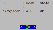
18.1.3 - Setting node type
When you create a node, Vertica automatically sets its type to PERMANENT.
When you create a node, Vertica automatically sets its type to PERMANENT. This enables Vertica to use this node to store data. You can change a node's type with
ALTER NODE, to one of the following:
-
PERMANENT: (default): A node that stores data.
-
EPHEMERAL: A node that is in transition from one type to another—typically, from PERMANENT to either STANDBY or EXECUTE.
-
STANDBY: A node that is reserved to replace any node when it goes down. A standby node stores no segments or data until it is called to replace a down node. When used as a replacement node, Vertica changes its type to PERMANENT. For more information, see Active standby nodes.
-
EXECUTE: A node that is reserved for computation purposes only. An execute node contains no segments or data.
Note
STANDBY and EXECUTE node types are supported only in Enterprise Mode.
18.1.4 - Active standby nodes
An active standby node exists is a node in an Enterprise Mode database that is available to replace any failed node.
An active standby node exists is a node in an Enterprise Mode database that is available to replace any failed node. Unlike permanent Vertica nodes, an standby node does not perform computations or contain data. If a permanent node fails, an active standby node can replace the failed node, after the failed node exceeds the failover time limit. After replacing the failed node, the active standby node contains the projections and performs all calculations of the node it replaced.
In this section
18.1.4.1 - Creating an active standby node
You can create active standby nodes in an Enterprise Mode database at the same time that you create the database, or later.
You can create active standby nodes in an Enterprise Mode database at the same time that you create the database, or later.
Note
When you create an active standby node, be sure to add any necessary storage locations. For more information, refer to
Adding Storage Locations.
Creating an active standby node in a new database
-
Create a database, including the nodes that you intend to use as active standby nodes.
-
Using vsql, connect to a node other than the node that you want to use as an active standby node.
-
Use ALTER NODE to convert the node from a permanent node to an active standby node. For example:
=> ALTER NODE v_mart_node5 STANDBY;
After you issue the ALTER NODE statement, the affected node goes down and restarts as an active standby node.
Creating an active standby node in an existing database
When you create a node to be used as an active standby node, change the new node to ephemeral status as quickly as possible to prevent the cluster from moving data to it.
-
Add a node to the database.
Important
Do not rebalance the database at this stage.
-
Using vsql, connect to any other node.
-
Use ALTER NODE to convert the new node from a permanent node to an ephemeral node. For example:
=> ALTER NODE v_mart_node5 EPHEMERAL;
-
Rebalance the cluster to remove all data from the ephemeral node.
-
Use ALTER NODE on the ephemeral node to convert it to an active standby node. For example:
=> ALTER NODE v_mart_node5 STANDBY;
18.1.4.2 - Replace a node with an active standby node
A failed node on an Enterprise Mode database can be replaced with an active standby node automatically, or manually.
A failed node on an Enterprise Mode database can be replaced with an active standby node automatically, or manually.
Important
A node must be down before it can be replaced with an active standby node. Attempts to replace a node that is up return with an error.
Automatic replacement
You can configure automatic replacement of failed nodes with parameter FailoverToStandbyAfter. If enabled, this parameter specifies the length of time that an active standby node waits before taking the place of a failed node. If possible, Vertica selects a standby node from the same fault group as the failed node. Otherwise, Vertica randomly selects an available active standby node.
Manual replacement
As an administrator, you can manually replace a failed node with ALTER NODE:
-
Connect to the database with Administration Tools or vsql.
-
Replace the node with ALTER NODE...REPLACE. The REPLACE option can specify a standby node. If REPLACE is unqualified, then Vertica selects a standby node from the same fault group as the failed node, if one is available; otherwise, it randomly selects an available active standby node.
18.1.4.3 - Revert active standby nodes
When a down node in an Enterprise Mode database is ready for reactivation, you can restore it by reverting its replacement to standby status.
When a down node in an Enterprise Mode database is ready for reactivation, you can restore it by reverting its replacement to standby status. You can perform this operation on individual nodes or the entire database, with ALTER NODE and ALTER DATABASE, respectively:
-
Connect to the database with Administration Tools or via vsql.
-
Revert the standby nodes.
-
Individually with ALTER NODE:
ALTER NODE node‑name RESET;
-
Collectively across the database cluster with ALTER DATABASE:
ALTER DATABASE DEFAULT RESET STANDBY;
If a down node cannot resume operation, Vertica ignores the reset request and leaves the standby node in place.
18.1.5 - Large cluster
Vertica uses the Spread service to broadcast control messages between database nodes.
Vertica uses the Spread service to broadcast control messages between database nodes. This service can limit the growth of a Vertica database cluster. As you increase the number of cluster nodes, the load on the Spread service also increases as more participants exchange messages. This increased load can slow overall cluster performance. Also, network addressing limits the maximum number of participants in the Spread service to 120 (and often far less). In this case, you can use large cluster to overcome these Spread limitations.
When large cluster is enabled, a subset of cluster nodes, called control nodes, exchange messages using the Spread service. Other nodes in the cluster are assigned to one of these control nodes, and depend on them for cluster-wide communication. Each control node passes messages from the Spread service to its dependent nodes. When a dependent node needs to broadcast a message to other nodes in the cluster, it passes the message to its control node, which in turn sends the message out to its other dependent nodes and the Spread service.

By setting up dependencies between control nodes and other nodes, you can grow the total number of database nodes, and remain in compliance with the Spread limit of 120 nodes.
Note
Technically, when large cluster is disabled, all of the nodes in the cluster are control nodes. In this case, all nodes connect to Spread. When large cluster is enabled, some nodes become dependent on control nodes.
A downside of the large cluster feature is that if a control node fails, its dependent nodes are cut off from the rest of the database cluster. These nodes cannot participate in database activities, and Vertica considers them to be down as well. When the control node recovers, it re-establishes communication between its dependent nodes and the database, so all of the nodes rejoin the cluster.
Note
The Spread service demon runs as an independent process on the control node host. It is not part of the Vertica process. If the Vertica process goes down on the node—for example, you use admintools to stop the Vertica process on the host—Spread continues to run. As long as the Spread demon runs on the control node, the node's dependents can communicate with the database cluster and participate in database activity. Normally, the control node only goes down if the node's host has an issue—or example, you shut it down, it becomes disconnected from the network, or a hardware failure occurs.
Large cluster and database growth
When your database has large cluster enabled, Vertica decides whether to make a newly added node into a control or a dependent node as follows:
-
In Enterprise Mode, if the number of control nodes configured for the database cluster is greater than the current number of nodes it contains, Vertica makes the new node a control node. In Eon Mode, the number of control nodes is set at the subcluster level. If the number of control nodes set for the subcluster containing the new node is less than this setting, Vertica makes the new node a control node.
-
If the Enterprise Mode cluster or Eon Mode subcluster has reached its limit on control nodes, a new node becomes a dependent of an existing control node.
When a newly-added node is a dependent node, Vertica automatically assigns it to a control node. Which control node it chooses is guided by the database mode:
-
Enterprise Mode database: Vertica assigns the new node to the control node with the least number of dependents. If you created fault groups in your database, Vertica chooses a control node in the same fault group as the new node. This feature lets you use fault groups to organize control nodes and their dependents to reflect the physical layout of the underlying host hardware. For example, you might want dependent nodes to be in the same rack as their control nodes. Otherwise, a failure that affects the entire rack (such as a power supply failure) will not only cause nodes in the rack to go down, but also nodes in other racks whose control node is in the affected rack. See Fault groups for more information.
-
Eon Mode database: Vertica always adds new nodes to a subcluster. Vertica assigns the new node to the control node with the fewest dependent nodes in that subcluster. Every subcluster in an Eon Mode database with large cluster enabled has at least one control node. Keeping dependent nodes in the same subcluster as their control node maintains subcluster isolation.
Important
In versions of Vertica prior to 10.0.1, nodes in an Eon Mode database with large cluster enabled were not necessarily assigned a control node in their subcluster. If you have upgraded your Eon Mode database from a version of Vertica earlier than 10.0.1 and have large cluster enabled, realign the control nodes in your database. This process reassigns dependent nodes and fixes any cross-subcluster control node dependencies. See
Realigning Control Nodes and Reloading Spread for more information.
Spread's upper limit of 120 participants can cause errors when adding a subcluster to an Eon Mode database. If your database cluster has 120 control nodes, attempting to create a subcluster fails with an error. Every subcluster must have at least one control node. When your cluster has 120 control nodes , Vertica cannot create a control node for the new subcluster. If this error occurs, you must reduce the number of control nodes in your database cluster before adding a subcluster.
When to enable large cluster
Vertica automatically enables large cluster in two cases:
-
The database cluster contains 120 or more nodes. This is true for both Enterprise Mode and Eon Mode.
-
You create an Eon Mode subcluster (either a primary subcluster or a secondary subcluster) with an initial node count of 16 or more.
Vertica does not automatically enable large cluster if you expand an existing subcluster to 16 or more nodes by adding nodes to it.
Note
You can prevent Vertica from automatically enabling large cluster when you create a subcluster with 16 or more nodes by setting the control-set-size parameter to -1. See
Creating subclusters for details.
You can choose to manually enable large cluster mode before Vertica automatically enables it. Your best practice is to enable large cluster when your database cluster size reaches a threshold:
-
For cloud-based databases, enable large cluster when the cluster contains 16 or more nodes. In a cloud environment, your database uses point-to-point network communications. Spread scales poorly in point-to-point communications mode. Enabling large cluster when the database cluster reaches 16 nodes helps limit the impact caused by Spread being in point-to-point mode.
-
For on-premises databases, enable large cluster when the cluster reaches 50 to 80 nodes. Spread scales better in an on-premises environment. However, by the time the cluster size reaches 50 to 80 nodes, Spread may begin exhibiting performance issues.
In either cloud or on-premises environments, enable large cluster if you begin to notice Spread-related performance issues. Symptoms of Spread performance issues include:
-
The load on the spread service begins to cause performance issues. Because Vertica uses Spread for cluster-wide control messages, Spread performance issues can adversely affect database performance. This is particularly true for cloud-based databases, where Spread performance problems becomes a bottleneck sooner, due to the nature of network broadcasting in the cloud infrastructure. In on-premises databases, broadcast messages are usually less of a concern because messages usually remain within the local subnet. Even so, eventually, Spread usually becomes a bottleneck before Vertica automatically enables large cluster automatically when the cluster reaches 120 nodes.
-
The compressed list of addresses in your cluster is too large to fit in a maximum transmission unit (MTU) packet (1478 bytes). The MTU packet has to contain all of the addresses for the nodes participating in the Spread service. Under ideal circumstances (when your nodes have the IP addresses 1.1.1.1, 1.1.1.2 and so on) 120 addresses can fit in this packet. This is why Vertica automatically enables large cluster if your database cluster reaches 120 nodes. In practice, the compressed list of IP addresses will reach the MTU packet size limit at 50 to 80 nodes.
18.1.5.1 - Planning a large cluster
There are two factors you should consider when planning to expand your database cluster to the point that it needs to use large cluster:.
There are two factors you should consider when planning to expand your database cluster to the point that it needs to use large cluster:
Determining the number of control nodes
When you manually enable large cluster or add enough nodes to trigger Vertica to enable it automatically, a subset of the cluster nodes become control nodes. In subclusters with fewer than 16 nodes, all nodes are control nodes. In many cases, you can set the number of control nodes to the square root of the total number of nodes in the entire Enterprise Mode cluster, or in Eon Mode subclusters with more than 16 nodes. However, this formula for calculating the number of control is not guaranteed to always meet your requirements.
When choosing the number of control nodes in a database cluster, you must balance two competing considerations:
-
If a control node fails or is shut down, all nodes that depend on it are cut off from the database. They are also down until the control node rejoins the database. You can reduce the impact of a control node failure by increasing the number of control nodes in your cluster.
-
The more control nodes in your cluster, the greater the load on the spread service. In cloud environments, increased complexity of the network environment broadcast can contribute to high latency. This latency can cause messages sent over the spread service to take longer to reach all of the nodes in the cluster.
In a cloud environment, experience has shown that 16 control nodes balances the needs of reliability and performance. In an Eon Mode database, you must have at least one control node per subcluster. Therefore, if you have more than 16 subclusters, you must have more than 16 control nodes.
In an Eon Mode database, whether on-premises or in the cloud, consider adding more control nodes to your primary subclusters than to secondary subclusters. Only nodes in primary subclusters are responsible for maintaining K-safety in an Eon Mode database. Therefore, a control node failure in a primary subcluster can have greater impact on your database than a control node failure in a secondary subcluster.
In an on-premises Enterprise Mode database, consider the physical layout of the hosts running your database when choosing the number of control nodes. If your hosts are spread across multiple server racks, you want to have enough control nodes to distribute them across the racks. Distributing the control nodes helps ensure reliability in the case of a failure that involves the entire rack (such as a power supply or network switch failure). You can configure your database so no node depends on a control node that is in a separate rack. Limiting dependency to within a rack prevents a failure that affects an entire rack from causing additional node loss outside the rack due to control node loss.
Selecting the number of control nodes based on the physical layout also lets you reduce network traffic across switches. By having dependent nodes on the same racks as their control nodes, the communications between them remain in the rack, rather that traversing a network switch.
You might need to increase the number of control nodes to evenly distribute them across your racks. For example, on-premises Enterprise Mode database has 64 total nodes, spread across three racks. The square root of the number of nodes yields 8 control nodes for this cluster. However, you cannot evenly distribute eight control nodes among the three racks. Instead, you can have 9 control nodes and evenly distribute three control nodes per rack.
Influencing control node placement
After you determine the number of nodes for your cluster, you need to determine how to distribute them among the cluster nodes. Vertica chooses which nodes become control nodes. You can influence how Vertica chooses the control nodes and which nodes become their dependents. The exact process you use depends on your database's mode:
-
Enterprise Mode on-premises database: Define fault groups to influence control node placement. Dependent nodes are always in the same fault group as their control node. You usually define fault groups that reflect the physical layout of the hosts running your database. For example, you usually define one or more fault groups for the nodes in a single rack of servers. When the fault groups reflect your physical layout, Vertica places control nodes and dependents in a way that can limit the impact of rack failures. See Fault groups for more information.
-
Eon Mode database: Use subclusters to control the placement of control nodes. Each subcluster must have at least one control node. Dependent nodes are always in the same subcluster as their control nodes. You can set the number of control nodes for each subcluster. Doing so lets you assign more control nodes to primary subclusters, where it's important to minimize the impact of a control node failure.
How Vertica chooses a default number of control nodes
Vertica can automatically choose the number of control nodes in the entire cluster (when in Enterprise Mode) or for a subcluster (when in Eon Mode). It sets a default value in these circumstances:
-
When you pass the default keyword to the --large-cluster option of the
install_vertica script (see Enable Large Cluster When Installing Vertica).
-
Vertica automatically enables large cluster when your database cluster grows to 120 or more nodes.
-
Vertica automatically enables large cluster for an Eon Mode subcluster if you create it with more than 16 nodes. Note that Vertica does not enable large cluster on a subcluster you expand past the 16 node limit. It only enables large clusters that start out larger than 16 nodes.
The number of control nodes Vertica chooses depends on what triggered Vertica to set the value.
If you pass the --large-cluster default option to the
install_vertica script, Vertica sets the number of control nodes to the square root of the number of nodes in the initial cluster.
If your database cluster reaches 120 nodes, Vertica enables large cluster by making any newly-added nodes into dependents. The default value for the limit on the number of control nodes is 120. When you reach this limit, any newly-added nodes are added as dependents. For example, suppose you have a 115 node Enterprise Mode database cluster where you have not manually enabled large cluster. If you add 10 nodes to this cluster, Vertica adds 5 of the nodes as control nodes (bringing you up to the 120-node limit) and the other 5 nodes as dependents.
Important
You should manually enable large cluster before your database reaches 120 nodes.
In an Eon Mode database, each subcluster has its own setting for the number of control nodes. Vertica only automatically sets the number of control nodes when you create a subcluster with more than 16 nodes initially. When this occurs, Vertica sets the number of control nodes for the subcluster to the square root of the number of nodes in the subcluster.
For example, suppose you add a new subcluster with 25 nodes in it. This subcluster starts with more than the 16 node limit, so Vertica sets the number of control nodes for subcluster to 5 (which is the square root of 25). Five of the nodes are added as control nodes, and the remaining 20 are added as dependents of those five nodes.
Even though each subcluster has its own setting for the number of control nodes, an Eon Mode database cluster still has the 120 node limit on the total number of control nodes that it can have.
18.1.5.2 - Enabling large cluster
Vertica enables the large cluster feature automatically when:.
Vertica enables the large cluster feature automatically when:
In most cases, you should consider manually enabling large cluster before your cluster size reaches either of these thresholds. See Planning a large cluster for guidance on when to enable large cluster.
You can enable large cluster on a new Vertica database, or on an existing database.
Enable large cluster when installing Vertica
You can enable large cluster when installing Vertica onto a new database cluster. This option is useful if you know from the beginning that your database will benefit from large cluster.
The install_vertica script's
‑‑large‑cluster argument enables large cluster during installation. It takes a single integer value between 1 and 120 that specifies the number of control nodes to create in the new database cluster. Alternatively, this option can take the literal argument default. In this case, Vertica enables large cluster mode and sets the number of control nodes to the square root of the number nodes you provide in the
‑‑hosts argument. For example, if ‑‑hosts specifies 25 hosts and ‑‑large‑cluster is set to default, the install script creates a database cluster with 5 control nodes.
The ‑‑large‑cluster argument has a slightly different effect depending on the database mode you choose when creating your database:
-
Enterprise Mode: ‑‑large‑cluster sets the total number of control nodes for the entire database cluster.
-
Eon Mode : ‑‑large‑cluster sets the number of control nodes in the initial default subcluster. This setting has no effect on subclusters that you create later.
Note
You cannot use ‑‑large‑cluster to set the number of control nodes in your initial database to be higher than the number of you pass in the ‑‑hosts argument. The installer sets the number of control nodes to whichever is the lower value: the value you pass to the ‑‑large‑cluster option or the number of hosts in the ‑‑hosts option.
You can set the number of control nodes to be higher than the number of nodes currently in an existing database, with the meta-function SET_CONTROL_SET_SIZE function. You choose to set a higher number to preallocate control nodes when planning for future expansion. For details, see Changing the number of control nodes and realigning.
After the installation process completes, use the Administration tools or the [%=Vertica.MC%] to create a database. See Create an empty database for details.
If your database is on-premises and running in Enterprise Mode, you usually want to define fault groups that reflect the physical layout of your hosts. They let you define which hosts are in the same server racks, and are dependent on the same infrastructure (such power supplies and network switches). With this knowledge, Vertica can realign the control nodes to make your database better able to cope with hardware failures. See Fault groups for more information.
After creating a database, any nodes that you add are, by default, dependent nodes. You can change the number of control nodes in the database with the meta-function SET_CONTROL_SET_SIZE.
Enable large cluster in an existing database
You can manually enable large cluster in an existing database. You usually choose to enable large cluster manually before your database reaches the point where Vertica automatically enables it. See When To Enable Large Cluster for an explanation of when you should consider enabling large cluster.
Use the meta-function SET_CONTROL_SET_SIZE to enable large cluster and set the number of control nodes. You pass this function an integer value that sets the number of control nodes in the entire Enterprise Mode cluster, or in an Eon Mode subcluster.
18.1.5.3 - Changing the number of control nodes and realigning
You can change the number of control nodes in the entire database cluster in Enterprise Mode, or the number of control nodes in a subcluster in Eon Mode.
You can change the number of control nodes in the entire database cluster in Enterprise Mode, or the number of control nodes in a subcluster in Eon Mode. You may choose to change the number of control nodes in a cluster or subcluster to reduce the impact of control node loss on your database. See Planning a large cluster to learn more about when you should change the number of control nodes in your database.
You change the number of control nodes by calling the meta-function SET_CONTROL_SET_SIZE. If large cluster was not enabled before the call to SET_CONTROL_SET_SIZE, the function enables large cluster in your database. See Enabling large cluster for more information.
When you call SET_CONTROL_SET_SIZE in an Enterprise Mode database, it sets the number of control nodes in the entire database cluster. In an Eon Mode database, you must supply SET_CONTROL_SET_SIZE with the name of a subcluster in addition to the number of control nodes. The function sets the number of control nodes for that subcluster. Other subclusters in the database cluster are unaffected by this call.
Before changing the number of control nodes in an Eon Mode subcluster, verify that the subcluster is running. Changing the number of control nodes of a subcluster while it is down can cause configuration issues that prevent nodes in the subcluster from starting.
Note
You can set the number of control nodes to a value that is higher than the number of nodes currently in the cluster or subcluster. When the number of control nodes is higher than the current node count, newly-added nodes become control nodes until the number of nodes in the cluster or subcluster reaches the number control nodes you set.
You may choose to set the number of control nodes higher than the current node count to plan for future expansion. For example, suppose you have a 4-node subcluster in an Eon Mode database that you plan to expand in the future. You determine that you want limit the number of control nodes in this cluster to 8, even if you expand it beyond that size. In this case, you can choose to set the control node size for the subcluster to 8 now. As you add new nodes to the subcluster, they become control nodes until the size of the subcluster reaches 8. After that point, Vertica assigns newly-added nodes as a dependent of an existing control node in the subcluster.
Realigning control nodes and reloading spread
After you call the SET_CONTROL_SET_SIZE function, there are several additional steps you must take before the new setting takes effect.
Important
Follow these steps if you have upgraded your large-cluster enabled Eon Mode database from a version prior to 10.0.1. Earlier versions of Vertica did not restrict control node assignments to be within the same subcluster. When you realign the control nodes after an upgrade, Vertica configures each subcluster to have at least one control node, and assigns nodes to a control node in their own subcluster.
-
Call the REALIGN_CONTROL_NODES function. This function tells Vertica to re-evaluate the assignment of control nodes and their dependents in your cluster or subcluster. When calling this function in an Eon Mode database, you must supply the name of the subcluster where you changed the control node settings.
-
Call the RELOAD_SPREAD function. This function updates the control node assignment information in configuration files and triggers Spread to reload.
-
Restart the nodes affected by the change in control nodes. In an Enterprise Mode database, you must restart the entire database to ensure all nodes have updated configuration information. In Eon Mode, restart the subcluster or subclusters affected by your changes. You must restart the entire Eon Mode database if you changed a critical subcluster (such as the only primary subcluster).
Note
You do not need to restart nodes if the earlier steps didn't change control node assignments. This case usually only happens when you set the number of control nodes in an Eon Mode subcluster to higher than the subcluster's current node count, and all nodes in the subcluster are already control nodes. In this case, no control nodes are added or removed, so node dependencies do not change. Because the dependencies did not change, the nodes do not need to reload the Spread configuration.
-
In an Enterprise Mode database, call START_REBALANCE_CLUSTER to rebalance the cluster. This process improves your database's fault tolerance by shifting buddy projection assignments to limit the impact of a control node failure. You do not need to take this step in an Eon Mode database.
Enterprise Mode example
The following example makes 4 out of the 8 nodes in an Enterprise Mode database into control nodes. It queries the LARGE_CLUSTER_CONFIGURATION_STATUS system table which shows control node assignments for each node in the database. At the start, all nodes are their own control nodes. See Monitoring large clusters for more information the system tables associated with large cluster.
=> SELECT * FROM V_CATALOG.LARGE_CLUSTER_CONFIGURATION_STATUS;
node_name | spread_host_name | control_node_name
------------------+------------------+-------------------
v_vmart_node0001 | v_vmart_node0001 | v_vmart_node0001
v_vmart_node0002 | v_vmart_node0002 | v_vmart_node0002
v_vmart_node0003 | v_vmart_node0003 | v_vmart_node0003
v_vmart_node0004 | v_vmart_node0004 | v_vmart_node0004
v_vmart_node0005 | v_vmart_node0005 | v_vmart_node0005
v_vmart_node0006 | v_vmart_node0006 | v_vmart_node0006
v_vmart_node0007 | v_vmart_node0007 | v_vmart_node0007
v_vmart_node0008 | v_vmart_node0008 | v_vmart_node0008
(8 rows)
=> SELECT SET_CONTROL_SET_SIZE(4);
SET_CONTROL_SET_SIZE
----------------------
Control size set
(1 row)
=> SELECT REALIGN_CONTROL_NODES();
REALIGN_CONTROL_NODES
---------------------------------------------------------------
The new control node assignments can be viewed in vs_nodes.
Check vs_cluster_layout to see the proposed new layout. Reboot
all the nodes and call rebalance_cluster now
(1 row)
=> SELECT RELOAD_SPREAD(true);
RELOAD_SPREAD
---------------
Reloaded
(1 row)
=> SELECT SHUTDOWN();
After restarting the database, the final step is to rebalance the cluster and query the LARGE_CLUSTER_CONFIGURATION_STATUS table to see the current control node assignments:
=> SELECT START_REBALANCE_CLUSTER();
START_REBALANCE_CLUSTER
-------------------------
REBALANCING
(1 row)
=> SELECT * FROM V_CATALOG.LARGE_CLUSTER_CONFIGURATION_STATUS;
node_name | spread_host_name | control_node_name
------------------+------------------+-------------------
v_vmart_node0001 | v_vmart_node0001 | v_vmart_node0001
v_vmart_node0002 | v_vmart_node0002 | v_vmart_node0002
v_vmart_node0003 | v_vmart_node0003 | v_vmart_node0003
v_vmart_node0004 | v_vmart_node0004 | v_vmart_node0004
v_vmart_node0005 | v_vmart_node0001 | v_vmart_node0001
v_vmart_node0006 | v_vmart_node0002 | v_vmart_node0002
v_vmart_node0007 | v_vmart_node0003 | v_vmart_node0003
v_vmart_node0008 | v_vmart_node0004 | v_vmart_node0004
(8 rows)
Eon Mode example
The following example configures 4 control nodes in an 8-node secondary subcluster named analytics. The primary subcluster is not changed. The primary differences between this example and the previous Enterprise Mode example is the need to specify a subcluster when calling SET_CONTROL_SET_SIZE, not having to restart the entire database, and not having to call START_REBALANCE_CLUSTER.
=> SELECT * FROM V_CATALOG.LARGE_CLUSTER_CONFIGURATION_STATUS;
node_name | spread_host_name | control_node_name
----------------------+----------------------+----------------------
v_verticadb_node0001 | v_verticadb_node0001 | v_verticadb_node0001
v_verticadb_node0002 | v_verticadb_node0002 | v_verticadb_node0002
v_verticadb_node0003 | v_verticadb_node0003 | v_verticadb_node0003
v_verticadb_node0004 | v_verticadb_node0004 | v_verticadb_node0004
v_verticadb_node0005 | v_verticadb_node0005 | v_verticadb_node0005
v_verticadb_node0006 | v_verticadb_node0006 | v_verticadb_node0006
v_verticadb_node0007 | v_verticadb_node0007 | v_verticadb_node0007
v_verticadb_node0008 | v_verticadb_node0008 | v_verticadb_node0008
v_verticadb_node0009 | v_verticadb_node0009 | v_verticadb_node0009
v_verticadb_node0010 | v_verticadb_node0010 | v_verticadb_node0010
v_verticadb_node0011 | v_verticadb_node0011 | v_verticadb_node0011
(11 rows)
=> SELECT subcluster_name,node_name,is_primary,control_set_size FROM
V_CATALOG.SUBCLUSTERS;
subcluster_name | node_name | is_primary | control_set_size
--------------------+----------------------+------------+------------------
default_subcluster | v_verticadb_node0001 | t | -1
default_subcluster | v_verticadb_node0002 | t | -1
default_subcluster | v_verticadb_node0003 | t | -1
analytics | v_verticadb_node0004 | f | -1
analytics | v_verticadb_node0005 | f | -1
analytics | v_verticadb_node0006 | f | -1
analytics | v_verticadb_node0007 | f | -1
analytics | v_verticadb_node0008 | f | -1
analytics | v_verticadb_node0009 | f | -1
analytics | v_verticadb_node0010 | f | -1
analytics | v_verticadb_node0011 | f | -1
(11 rows)
=> SELECT SET_CONTROL_SET_SIZE('analytics',4);
SET_CONTROL_SET_SIZE
----------------------
Control size set
(1 row)
=> SELECT REALIGN_CONTROL_NODES('analytics');
REALIGN_CONTROL_NODES
-----------------------------------------------------------------------------
The new control node assignments can be viewed in vs_nodes. Call
reload_spread(true). If the subcluster is critical, restart the database.
Otherwise, restart the subcluster
(1 row)
=> SELECT RELOAD_SPREAD(true);
RELOAD_SPREAD
---------------
Reloaded
(1 row)
At this point, the analytics subcluster needs to restart. You have several options to restart it. See Starting and stopping subclusters for details. This example uses the admintools command line to stop and start the subcluster.
$ admintools -t stop_subcluster -d verticadb -c analytics -p password
*** Forcing subcluster shutdown ***
Verifying subcluster 'analytics'
Node 'v_verticadb_node0004' will shutdown
Node 'v_verticadb_node0005' will shutdown
Node 'v_verticadb_node0006' will shutdown
Node 'v_verticadb_node0007' will shutdown
Node 'v_verticadb_node0008' will shutdown
Node 'v_verticadb_node0009' will shutdown
Node 'v_verticadb_node0010' will shutdown
Node 'v_verticadb_node0011' will shutdown
Shutdown subcluster command successfully sent to the database
$ admintools -t restart_subcluster -d verticadb -c analytics -p password
*** Restarting subcluster for database verticadb ***
Restarting host [10.11.12.19] with catalog [v_verticadb_node0004_catalog]
Restarting host [10.11.12.196] with catalog [v_verticadb_node0005_catalog]
Restarting host [10.11.12.51] with catalog [v_verticadb_node0006_catalog]
Restarting host [10.11.12.236] with catalog [v_verticadb_node0007_catalog]
Restarting host [10.11.12.103] with catalog [v_verticadb_node0008_catalog]
Restarting host [10.11.12.185] with catalog [v_verticadb_node0009_catalog]
Restarting host [10.11.12.80] with catalog [v_verticadb_node0010_catalog]
Restarting host [10.11.12.47] with catalog [v_verticadb_node0011_catalog]
Issuing multi-node restart
Starting nodes:
v_verticadb_node0004 (10.11.12.19) [CONTROL]
v_verticadb_node0005 (10.11.12.196) [CONTROL]
v_verticadb_node0006 (10.11.12.51) [CONTROL]
v_verticadb_node0007 (10.11.12.236) [CONTROL]
v_verticadb_node0008 (10.11.12.103)
v_verticadb_node0009 (10.11.12.185)
v_verticadb_node0010 (10.11.12.80)
v_verticadb_node0011 (10.11.12.47)
Starting Vertica on all nodes. Please wait, databases with a large catalog may take a while to initialize.
Node Status: v_verticadb_node0004: (DOWN) v_verticadb_node0005: (DOWN) v_verticadb_node0006: (DOWN)
v_verticadb_node0007: (DOWN) v_verticadb_node0008: (DOWN) v_verticadb_node0009: (DOWN)
v_verticadb_node0010: (DOWN) v_verticadb_node0011: (DOWN)
Node Status: v_verticadb_node0004: (DOWN) v_verticadb_node0005: (DOWN) v_verticadb_node0006: (DOWN)
v_verticadb_node0007: (DOWN) v_verticadb_node0008: (DOWN) v_verticadb_node0009: (DOWN)
v_verticadb_node0010: (DOWN) v_verticadb_node0011: (DOWN)
Node Status: v_verticadb_node0004: (INITIALIZING) v_verticadb_node0005: (INITIALIZING) v_verticadb_node0006:
(INITIALIZING) v_verticadb_node0007: (INITIALIZING) v_verticadb_node0008: (INITIALIZING)
v_verticadb_node0009: (INITIALIZING) v_verticadb_node0010: (INITIALIZING) v_verticadb_node0011: (INITIALIZING)
Node Status: v_verticadb_node0004: (UP) v_verticadb_node0005: (UP) v_verticadb_node0006: (UP)
v_verticadb_node0007: (UP) v_verticadb_node0008: (UP) v_verticadb_node0009: (UP)
v_verticadb_node0010: (UP) v_verticadb_node0011: (UP)
Syncing catalog on verticadb with 2000 attempts.
Once the subcluster restarts, you can query the system tables to see the control node configuration:
=> SELECT * FROM V_CATALOG.LARGE_CLUSTER_CONFIGURATION_STATUS;
node_name | spread_host_name | control_node_name
----------------------+----------------------+----------------------
v_verticadb_node0001 | v_verticadb_node0001 | v_verticadb_node0001
v_verticadb_node0002 | v_verticadb_node0002 | v_verticadb_node0002
v_verticadb_node0003 | v_verticadb_node0003 | v_verticadb_node0003
v_verticadb_node0004 | v_verticadb_node0004 | v_verticadb_node0004
v_verticadb_node0005 | v_verticadb_node0005 | v_verticadb_node0005
v_verticadb_node0006 | v_verticadb_node0006 | v_verticadb_node0006
v_verticadb_node0007 | v_verticadb_node0007 | v_verticadb_node0007
v_verticadb_node0008 | v_verticadb_node0004 | v_verticadb_node0004
v_verticadb_node0009 | v_verticadb_node0005 | v_verticadb_node0005
v_verticadb_node0010 | v_verticadb_node0006 | v_verticadb_node0006
v_verticadb_node0011 | v_verticadb_node0007 | v_verticadb_node0007
(11 rows)
=> SELECT subcluster_name,node_name,is_primary,control_set_size FROM subclusters;
subcluster_name | node_name | is_primary | control_set_size
--------------------+----------------------+------------+------------------
default_subcluster | v_verticadb_node0001 | t | -1
default_subcluster | v_verticadb_node0002 | t | -1
default_subcluster | v_verticadb_node0003 | t | -1
analytics | v_verticadb_node0004 | f | 4
analytics | v_verticadb_node0005 | f | 4
analytics | v_verticadb_node0006 | f | 4
analytics | v_verticadb_node0007 | f | 4
analytics | v_verticadb_node0008 | f | 4
analytics | v_verticadb_node0009 | f | 4
analytics | v_verticadb_node0010 | f | 4
analytics | v_verticadb_node0011 | f | 4
(11 rows)
Disabling large cluster
To disable large cluster, call SET_CONTROL_SET_SIZE with a value of -1. This value is the default for non-large cluster databases. It tells Vertica to make all nodes into control nodes.
In an Eon Mode database, to fully disable large cluster you must to set the number of control nodes to -1 in every subcluster that has a set number of control nodes. You can see which subclusters have a set number of control nodes by querying the CONTROL_SET_SIZE column of the V_CATALOG.SUBCLUSTERS system table.
The following example resets the number of control nodes set in the previous Eon Mode example.
=> SELECT subcluster_name,node_name,is_primary,control_set_size FROM subclusters;
subcluster_name | node_name | is_primary | control_set_size
--------------------+----------------------+------------+------------------
default_subcluster | v_verticadb_node0001 | t | -1
default_subcluster | v_verticadb_node0002 | t | -1
default_subcluster | v_verticadb_node0003 | t | -1
analytics | v_verticadb_node0004 | f | 4
analytics | v_verticadb_node0005 | f | 4
analytics | v_verticadb_node0006 | f | 4
analytics | v_verticadb_node0007 | f | 4
analytics | v_verticadb_node0008 | f | 4
analytics | v_verticadb_node0009 | f | 4
analytics | v_verticadb_node0010 | f | 4
analytics | v_verticadb_node0011 | f | 4
(11 rows)
=> SELECT SET_CONTROL_SET_SIZE('analytics',-1);
SET_CONTROL_SET_SIZE
----------------------
Control size set
(1 row)
=> SELECT REALIGN_CONTROL_NODES('analytics');
REALIGN_CONTROL_NODES
---------------------------------------------------------------------------------------
The new control node assignments can be viewed in vs_nodes. Call reload_spread(true).
If the subcluster is critical, restart the database. Otherwise, restart the subcluster
(1 row)
=> SELECT RELOAD_SPREAD(true);
RELOAD_SPREAD
---------------
Reloaded
(1 row)
-- After restarting the analytics subcluster...
=> SELECT * FROM V_CATALOG.LARGE_CLUSTER_CONFIGURATION_STATUS;
node_name | spread_host_name | control_node_name
----------------------+----------------------+----------------------
v_verticadb_node0001 | v_verticadb_node0001 | v_verticadb_node0001
v_verticadb_node0002 | v_verticadb_node0002 | v_verticadb_node0002
v_verticadb_node0003 | v_verticadb_node0003 | v_verticadb_node0003
v_verticadb_node0004 | v_verticadb_node0004 | v_verticadb_node0004
v_verticadb_node0005 | v_verticadb_node0005 | v_verticadb_node0005
v_verticadb_node0006 | v_verticadb_node0006 | v_verticadb_node0006
v_verticadb_node0007 | v_verticadb_node0007 | v_verticadb_node0007
v_verticadb_node0008 | v_verticadb_node0008 | v_verticadb_node0008
v_verticadb_node0009 | v_verticadb_node0009 | v_verticadb_node0009
v_verticadb_node0010 | v_verticadb_node0010 | v_verticadb_node0010
v_verticadb_node0011 | v_verticadb_node0011 | v_verticadb_node0011
(11 rows)
=> SELECT subcluster_name,node_name,is_primary,control_set_size FROM subclusters;
subcluster_name | node_name | is_primary | control_set_size
--------------------+----------------------+------------+------------------
default_subcluster | v_verticadb_node0001 | t | -1
default_subcluster | v_verticadb_node0002 | t | -1
default_subcluster | v_verticadb_node0003 | t | -1
analytics | v_verticadb_node0004 | f | -1
analytics | v_verticadb_node0005 | f | -1
analytics | v_verticadb_node0006 | f | -1
analytics | v_verticadb_node0007 | f | -1
analytics | v_verticadb_node0008 | f | -1
analytics | v_verticadb_node0009 | f | -1
analytics | v_verticadb_node0010 | f | -1
analytics | v_verticadb_node0011 | f | -1
(11 rows)
18.1.5.4 - Monitoring large clusters
Monitor large cluster traits by querying the following system tables:.
Monitor large cluster traits by querying the following system tables:
-
V_CATALOG.LARGE_CLUSTER_CONFIGURATION_STATUS—Shows the current spread hosts and the control designations in the catalog so you can see if they match.
-
V_MONITOR.CRITICAL_HOSTS—Lists the hosts whose failure would cause the database to become unsafe and force a shutdown.
Tip
The CRITICAL_HOSTS view is especially useful for large cluster arrangements. For non-large clusters, query the
CRITICAL_NODES table.
-
In an Eon Mode database, the CONTROL_SET_SIZE column of the V_CATALOG.SUBCLUSTERS system table shows the number of control nodes set for each subcluster.
You might also want to query the following system tables:
-
V_CATALOG.FAULT_GROUPS—Shows fault groups and their hierarchy in the cluster.
-
V_CATALOG.CLUSTER_LAYOUT—Shows the relative position of the actual arrangement of the nodes participating in the database cluster and the fault groups that affect them.
18.1.6 - Multiple databases on a cluster
Vertica allows you to manage your database workloads by running multiple databases on a single cluster.
Vertica allows you to manage your database workloads by running multiple databases on a single cluster. However, databases cannot share the same node while running.
Example
If you have an 8-node cluster, with database 1 running on nodes 1, 2, 3, 4 and database 2 running on nodes 5, 6, 7, 8, you cannot create a new database in this cluster because all nodes are occupied. But if you stop database 1, you can create a database 3 using nodes 1, 2, 3, 4. Or if you stop both databases 1 and 2, you can create a database 3 using nodes 3, 4, 5, 6. In this latter case, database 1 and database 2 cannot be restarted unless you stop database 3, as they occupy the same nodes.
18.1.7 - Fault groups
You cannot create fault groups for an Eon Mode database.
Note
You cannot create fault groups for an Eon Mode database. Rather, Vertica automatically creates fault groups on a large cluster Eon database; these fault groups are configured around the control nodes and their dependents of each subcluster. These fault groups are managed internally by Vertica and are not accessible to users.
Fault groups let you configure an Enterprise Mode database for your physical cluster layout. Sharing your cluster topology lets you use terrace routing to reduce the buffer requirements of large queries. It also helps to minimize the risk of correlated failures inherent in your environment, usually caused by shared resources.
Vertica automatically creates fault groups around
control nodes (servers that run spread) in large cluster arrangements, placing nodes that share a control node in the same fault group. Automatic and user-defined fault groups do not include ephemeral nodes because such nodes hold no data.
Consider defining your own fault groups specific to your cluster's physical layout if you want to:
-
Use terrace routing to reduce the buffer requirements of large queries.
-
Reduce the risk of correlated failures. For example, by defining your rack layout, Vertica can better tolerate a rack failure.
-
Influence the placement of control nodes in the cluster.
Vertica supports complex, hierarchical fault groups of different shapes and sizes. The database platform provides a fault group script (DDL generator), SQL statements, system tables, and other monitoring tools.
See High availability with fault groups for an overview of fault groups with a cluster topology example.
18.1.7.1 - About the fault group script
To help you define fault groups on your cluster, Vertica provides a script named fault_group_ddl_generator.py in the /opt//scripts directory.
To help you define fault groups on your cluster, Vertica provides a script named fault_group_ddl_generator.py in the
/opt/vertica/scripts directory. This script generates the SQL statements you need to run to create fault groups.
The fault_group_ddl_generator.py script does not create fault groups for you, but you can copy the output to a file. Then, when you run the helper script, you can use \i or vsql–f commands to pass the cluster topology to Vertica.
The fault group script takes the following arguments:
For example:
$ python /opt/vertica/scripts/fault_group_ddl_generator.py VMartdb fault_grp_input.out
See also
18.1.7.2 - Creating a fault group input file
Use a text editor to create a fault group input file for the targeted cluster.
Use a text editor to create a fault group input file for the targeted cluster.
The following example shows how you can create a fault group input file for a cluster that has 8 racks with 8 nodes on each rack—for a total of 64 nodes in the cluster.
-
On the first line of the file, list the parent (top-level) fault groups, delimited by spaces.
rack1 rack2 rack3 rack4 rack5 rack6 rack7 rack8
-
On the subsequent lines, list the parent fault group followed by an equals sign (=). After the equals sign, list the nodes or fault groups delimited by spaces.
<parent> = <child_1> <child_2> <child_n...>
Such as:
rack1 = v_vmart_node0001 v_vmart_node0002 v_vmart_node0003 v_vmart_node0004
rack2 = v_vmart_node0005 v_vmart_node0006 v_vmart_node0007 v_vmart_node0008
rack3 = v_vmart_node0009 v_vmart_node0010 v_vmart_node0011 v_vmart_node0012
rack4 = v_vmart_node0013 v_vmart_node0014 v_vmart_node0015 v_vmart_node0016
rack5 = v_vmart_node0017 v_vmart_node0018 v_vmart_node0019 v_vmart_node0020
rack6 = v_vmart_node0021 v_vmart_node0022 v_vmart_node0023 v_vmart_node0024
rack7 = v_vmart_node0025 v_vmart_node0026 v_vmart_node0027 v_vmart_node0028
rack8 = v_vmart_node0029 v_vmart_node0030 v_vmart_node0031 v_vmart_node0032
After the first row of parent fault groups, the order in which you write the group descriptions does not matter. All fault groups that you define in this file must refer back to a parent fault group. You can indicate the parent group directly or by specifying the child of a fault group that is the child of a parent fault group.
Such as:
rack1 rack2 rack3 rack4 rack5 rack6 rack7 rack8
rack1 = v_vmart_node0001 v_vmart_node0002 v_vmart_node0003 v_vmart_node0004
rack2 = v_vmart_node0005 v_vmart_node0006 v_vmart_node0007 v_vmart_node0008
rack3 = v_vmart_node0009 v_vmart_node0010 v_vmart_node0011 v_vmart_node0012
rack4 = v_vmart_node0013 v_vmart_node0014 v_vmart_node0015 v_vmart_node0016
rack5 = v_vmart_node0017 v_vmart_node0018 v_vmart_node0019 v_vmart_node0020
rack6 = v_vmart_node0021 v_vmart_node0022 v_vmart_node0023 v_vmart_node0024
rack7 = v_vmart_node0025 v_vmart_node0026 v_vmart_node0027 v_vmart_node0028
rack8 = v_vmart_node0029 v_vmart_node0030 v_vmart_node0031 v_vmart_node0032
After you create your fault group input file, you are ready to run the fault_group_ddl_generator.py. This script generates the DDL statements you need to create fault groups in Vertica.
If your Vertica database is co-located on a Hadoop cluster, and that cluster uses more than one rack, you can use fault groups to improve performance. See Configuring rack locality.
See also
Creating fault groups
18.1.7.3 - Creating fault groups
When you define fault groups, Vertica distributes data segments across the cluster.
When you define fault groups, Vertica distributes data segments across the cluster. This allows the cluster to be aware of your cluster topology so it can tolerate correlated failures inherent in your environment, such as a rack failure. For an overview, see High Availability With Fault Groups.
Important
Defining fault groups requires careful and thorough network planning, and a solid understanding of your network topology.
Prerequisites
To define a fault group, you must have:
Run the fault group script
-
As the database administrator, run the fault_group_ddl_generator.py script:
python /opt/vertica/scripts/fault_group_ddl_generator.py databasename fault-group-inputfile > sql‑filename
For example, the following command writes the Python script output to the SQL file fault_group_ddl.sql.
$ python /opt/vertica/scripts/fault_group_ddl_generator.py
VMart fault_groups_VMart.out > fault_group_ddl.sql
After the script returns, you can run the SQL file, instead of multiple DDL statements individually.
Tip
Consider saving the input file so you can modify fault groups later—for example, after expanding the cluster or changing the distribution of control nodes.
-
Using vsql, run the DDL statements in fault_group_ddl.sql or execute the commands in the file using vsql.
=> \i fault_group_ddl.sql
-
If large cluster is enabled, realign control nodes with REALIGN_CONTROL_NODES. Otherwise, skip this step.
=> SELECT REALIGN_CONTROL_NODES();
-
Save cluster changes to the Spread configuration file by calling RELOAD_SPREAD:
=> SELECT RELOAD_SPREAD(true);
-
Use Administration tools to restart the database.
-
Save changes to the cluster's data layout by calling REBALANCE_CLUSTER:
=> SELECT REBALANCE_CLUSTER();
See also
18.1.7.4 - Monitoring fault groups
You can monitor fault groups by querying Vertica system tables or by logging in to the Management Console (MC) interface.
You can monitor fault groups by querying Vertica system tables or by logging in to the Management Console (MC) interface.
Monitor fault groups using system tables
Use the following system tables to view information about fault groups and cluster vulnerabilities, such as the nodes the cluster cannot lose without the database going down:
-
V_CATALOG.FAULT_GROUPS: View the hierarchy of all fault groups in the cluster.
-
V_CATALOG.CLUSTER_LAYOUT: Observe the arrangement of the nodes participating in the data business and the fault groups that affect them. Ephemeral nodes do not appear in the cluster layout ring because they hold no data.
Monitoring fault groups using Management Console
An MC administrator can monitor and highlight fault groups of interest by following these steps:
-
Click the running database you want to monitor and click Manage in the task bar.
-
Open the Fault Group View menu, and select the fault groups you want to view.
-
(Optional) Hide nodes that are not in the selected fault group to focus on fault groups of interest.
Nodes assigned to a fault group each have a colored bubble attached to the upper-left corner of the node icon. Each fault group has a unique color.If the number of fault groups exceeds the number of colors available, MC recycles the colors used previously.
Because Vertica supports complex, hierarchical fault groups of different shapes and sizes, MC displays multiple fault group participation as a stack of different-colored bubbles. The higher bubbles represent a lower-tiered fault group, which means that bubble is closer to the parent fault group, not the child or grandchild fault group.
For more information about fault group hierarchy, see High Availability With Fault Groups.
18.1.7.5 - Dropping fault groups
When you remove a fault group from the cluster, be aware that the drop operation removes the specified fault group and its child fault groups.
When you remove a fault group from the cluster, be aware that the drop operation removes the specified fault group and its child fault groups. Vertica places all nodes under the parent of the dropped fault group. To see the current fault group hierarchy in the cluster, query system table
FAULT_GROUPS.
Drop a fault group
Use the DROP FAULT GROUP statement to remove a fault group from the cluster. The following example shows how you can drops the group2 fault group:
=> DROP FAULT GROUP group2;
DROP FAULT GROUP
Drop all fault groups
Use the ALTER DATABASE statement to drop all fault groups, along with any child fault groups, from the specified database cluster.
The following command drops all fault groups from the current database.
=> ALTER DATABASE DEFAULT DROP ALL FAULT GROUP;
ALTER DATABASE
Add nodes back to a fault group
To add a node back to a fault group, you must manually reassign it to a new or existing fault group. To do so, use the CREATE FAULT GROUP and ALTER FAULT GROUP..ADD NODE statements.
See also
18.1.8 - Terrace routing
Before you apply terrace routing to your database, be sure you are familiar with large cluster and fault groups.
Terrace routing can significantly reduce message buffering on a large cluster database. The following sections describe how Vertica implements terrace routing on Enterprise Mode and Eon Mode databases.
Terrace routing on Enterprise Mode
Terrace routing on an Enterprise Mode database is implemented through fault groups that define a rack-based topology. In a large cluster with terrace routing disabled, nodes in a Vertica cluster form a fully connected network, where each non-dependent (control) node sends messages across the database cluster through connections with all other non-dependent nodes, both within and outside its own rack/fault group:
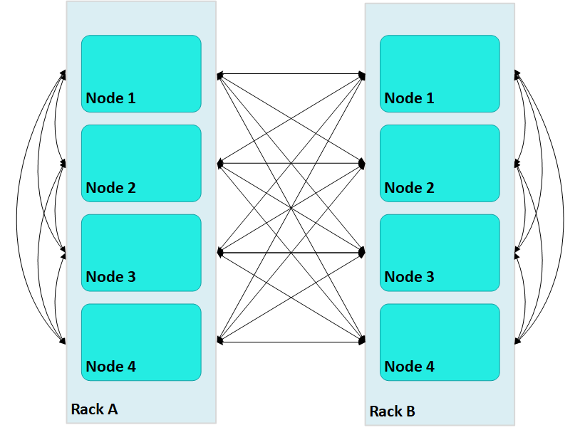
In this case, large Vertica clusters can require many connections on each node, where each connection incurs its own network buffering requirements. The total number of buffers required for each node is calculated as follows:
(numRacks * numRackNodes) - 1
In a two-rack cluster with 4 nodes per rack as shown above, this resolves to 7 buffers for each node.
With terrace routing enabled, you can considerably reduce large cluster network buffering. Each nth node in a rack/fault group is paired with the corresponding nth node of all other fault groups. For example, with terrace routing enabled, messaging in the same two-rack cluster is now implemented as follows:
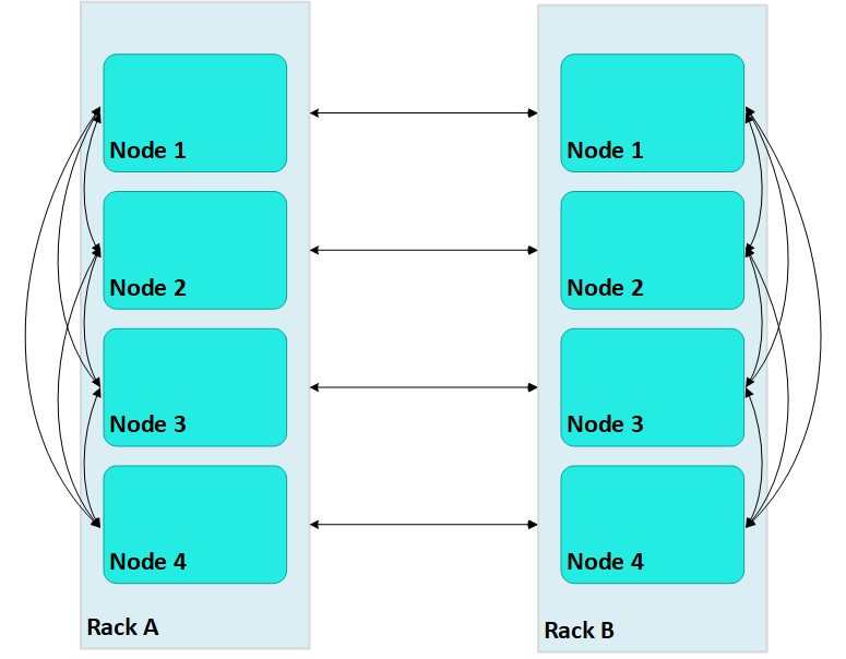
Thus, a message that originates from node 2 on rack A (A2) is sent to all other nodes on rack A; each rack A node then conveys the message to its corresponding node on rack B—A1 to B1, A2 to B2, and so on.
With terrace routing enabled, each node of a given rack avoids the overhead of maintaining message buffers to all other nodes. Instead, each node is only responsible for maintaining connections to:
Thus, the total number of message buffers required for each node is calculated as follows:
(numRackNodes-1) + (numRacks-1)
In a two-rack cluster with 4 nodes as shown earlier, this resolves to 4 buffers for each node.
Terrace routing trades time (intra-rack hops) for space (network message buffers). As a cluster expands with additional racks and nodes, the argument favoring this trade off becomes increasingly persuasive:
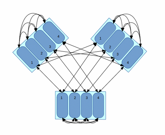
In this three-rack cluster with 4 nodes per rack, without terrace routing the number of buffers required by each node would be 11. With terrace routing, the number of buffers per node is 5. As a cluster expands with the addition of racks and nodes per rack, the disparity between buffer requirements widens. For example, given a six-rack cluster with 16 nodes per rack, without terrace routing the number of buffers required per node is 95; with terrace routing, 20.
Enabling terrace routing
Terrace routing depends on fault group definitions that describe a cluster network topology organized around racks and their member nodes. As noted earlier, when terrace routing is enabled, Vertica first distributes data within the rack/fault group; it then uses nth node-to-nth node mappings to forward this data to all other racks in the database cluster.
You enable (or disable) terrace routing for any Enterprise Mode large cluster that implements rack-based fault groups through configuration parameter TerraceRoutingFactor. To enable terrace routing, set this parameter as follows:
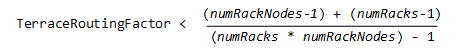
where:
For example:
|
#Racks |
Nodes/rack |
#Connections |
Terrace routing enabled if
TerraceRoutingFactor less than: |
|
Without terrace routing |
With terrace routing |
|
2 |
16 |
31 |
16 |
1.94 |
|
4 |
16 |
63 |
18 |
3.5 |
|
6 |
16 |
95 |
20 |
4.75 |
|
8 |
16 |
127 |
22 |
5.77 |
By default, TerraceRoutingFactor is set to 2, which generally ensures that terrace routing is enabled for any Enterprise Mode large cluster that implements rack-based fault groups. Vertica recommends enabling terrace routing for any cluster that contains 64 or more nodes, or if queries often require excessive buffer space.
To disable terrace routing, set TerraceRoutingFactor to a large integer such as 1000:
=> ALTER DATABASE DEFAULT SET TerraceRoutingFactor = 1000;
Terrace routing on Eon Mode
As in Enterprise Mode mode, terrace routing is enabled by default on an Eon Mode database, and is implemented through fault groups. However, you do not create fault groups for an Eon Mode database. Rather, Vertica automatically creates fault groups on a large cluster database; these fault groups are configured around the control nodes and their dependents of each subcluster. These fault groups are managed internally by Vertica and are not accessible to users.
18.1.9 - Elastic cluster
Elastic Cluster is an Enterprise Mode-only feature.
You can scale your cluster up or down to meet the needs of your database. The most common case is to add nodes to your database cluster to accommodate more data and provide better query performance. However, you can scale down your cluster if you find that it is over-provisioned, or if you need to divert hardware for other uses.
You scale your cluster by adding or removing nodes. Nodes can be added or removed without shutting down or restarting the database. After adding a node or before removing a node, Vertica begins a rebalancing process that moves data around the cluster to populate the new nodes or move data off nodes about to be removed from the database. During this process, nodes can exchange data that are not being added or removed to maintain robust intelligent K-safety. If Vertica determines that the data cannot be rebalanced in a single iteration due to lack of disk space, then the rebalance operation spans multiple iterations.
To help make data rebalancing due to cluster scaling more efficient, Vertica locally segments data storage on each node so it can be easily moved to other nodes in the cluster. When a new node is added to the cluster, existing nodes in the cluster give up some of their data segments to populate the new node. They also exchange segments to minimize the number of nodes that any one node depends upon. This strategy minimizes the number of nodes that might become critical when a node fails. When a node is removed from the cluster, its storage containers are moved to other nodes in the cluster (which also relocates data segments to minimize how many nodes might become critical when a node fails). This method of breaking data into portable segments is referred to as elastic cluster, as it facilitates enlarging or shrinking the cluster.
The alternative to elastic cluster is re-segmenting all projection data and redistributing it evenly among all database nodes any time a node is added or removed. This method requires more processing and more disk space, as it requires all data in all projections to be dumped and reloaded.
Elastic cluster scaling factor
In a new installation, each node has a scaling factor that specifies the number of local segments (see Scaling factor). Rebalance efficiently redistributes data by relocating local segments provided that, after nodes are added or removed, there are sufficient local segments in the cluster to redistribute the data evenly (determined by MAXIMUM_SKEW_PERCENT). For example, if the scaling factor = 8, and there are initially 5 nodes, then there are a total of 40 local segments cluster-wide.
If you add two additional nodes (seven nodes) Vertica relocates five local segments on two nodes, and six such segments on five nodes, resulting in roughly a 16.7 percent skew. Rebalance relocates local segments only if the resulting skew is less than the allowed threshold, as determined by MAXIMUM_SKEW_PERCENT. Otherwise, segmentation space (and hence data, if uniformly distributed over this space) is evenly distributed among the seven nodes, and new local segment boundaries are drawn for each node, such that each node again has eight local segments.
Note
By default, the scaling factor only has an effect while Vertica rebalances the database. While rebalancing, each node breaks the projection segments it contains into storage containers, which it then moves to other nodes if necessary. After rebalancing, the data is recombined into
ROS containers. It is possible to have Vertica always group data into storage containers. See
Local data segmentation for more information.
Enabling elastic cluster
You enable elastic cluster with ENABLE_ELASTIC_CLUSTER. Query the ELASTIC_CLUSTER system table to verify that elastic cluster is enabled:
=> SELECT is_enabled FROM ELASTIC_CLUSTER;
is_enabled
------------
t
(1 row)
18.1.9.1 - Scaling factor
To avoid an increased number of ROS containers, do not enable local segmentation and do not change the scaling factor.
To avoid an increased number of ROS containers, do not enable local segmentation and do not change the scaling factor.
18.1.9.2 - Viewing scaling factor settings
To view the scaling factor, query the ELASTIC_CLUSTER table:.
To view the scaling factor, query the ELASTIC_CLUSTER table:
=> SELECT scaling_factor FROM ELASTIC_CLUSTER;
scaling_factor
---------------
4
(1 row)
=> SELECT SET_SCALING_FACTOR(6);
SET_SCALING_FACTOR
--------------------
SET
(1 row)
=> SELECT scaling_factor FROM ELASTIC_CLUSTER;
scaling_factor
---------------
6
(1 row)
18.1.9.3 - Setting the scaling factor
Use the SET_SCALING_FACTOR function to change your database's scaling factor.
The scaling factor determines the number of storage containers that Vertica uses to store each projection across the database during rebalancing when local segmentation is enabled. When setting the scaling factor, follow these guidelines:
-
The number of storage containers should be greater than or equal to the number of partitions multiplied by the number of local segments:
num‑storage‑containers>= (num‑partitions*num‑local‑segments )
-
Set the scaling factor high enough so rebalance can transfer local segments to satisfy the skew threshold, but small enough so the number of storage containers does not result in too many ROS containers, and cause ROS pushback. The maximum number of ROS containers (by default 1024) is set by configuration parameter ContainersPerProjectionLimit.
Use the SET_SCALING_FACTOR function to change your database's scaling factor. The scaling factor can be an integer between 1 and 32.
=> SELECT SET_SCALING_FACTOR(12);
SET_SCALING_FACTOR
--------------------
SET
(1 row)
18.1.9.4 - Local data segmentation
By default, the scaling factor only has an effect when Vertica rebalances the database.
By default, the scaling factor only has an effect when Vertica rebalances the database. During rebalancing, nodes break the projection segments they contain into storage containers which they can quickly move to other nodes.
This process is more efficient than re-segmenting the entire projection (in particular, less free disk space is required), but it still has significant overhead, since storage containers have to be separated into local segments, some of which are then transferred to other nodes. This overhead is not a problem if you rarely add or remove nodes from your database.
However, if your database is growing rapidly and is constantly busy, you may find the process of adding nodes becomes disruptive. In this case, you can enable local segmentation, which tells Vertica to always segment its data based on the scaling factor, so the data is always broken into containers that are easily moved. Having the data segmented in this way dramatically speeds up the process of adding or removing nodes, since the data is always in a state that can be quickly relocated to another node. The rebalancing process that Vertica performs after adding or removing a node just has to decide which storage containers to relocate, instead of first having to first break the data into storage containers.
Local data segmentation increases the number of storage containers stored on each node. This is not an issue unless a table contains many partitions. For example, if the table is partitioned by day and contains one or more years. If local data segmentation is enabled, then each of these table partitions is broken into multiple local storage segments, which potentially results in a huge number of files which can lead to ROS "pushback." Consider your table partitions and the effect enabling local data segmentation may have before enabling the feature.
18.1.9.4.1 - Enabling and disabling local segmentation
To enable local segmentation, use the ENABLE_LOCAL_SEGMENTS function.
To enable local segmentation, use the ENABLE_LOCAL_SEGMENTS function. To disable local segmentation, use the DISABLE_LOCAL_SEGMENTATION function:
=> SELECT ENABLE_LOCAL_SEGMENTS();
ENABLE_LOCAL_SEGMENTS
-----------------------
ENABLED
(1 row)
=> SELECT is_local_segment_enabled FROM elastic_cluster;
is_enabled
------------
t
(1 row)
=> SELECT DISABLE_LOCAL_SEGMENTS();
DISABLE_LOCAL_SEGMENTS
------------------------
DISABLED
(1 row)
=> SELECT is_local_segment_enabled FROM ELASTIC_CLUSTER;
is_enabled
------------
f
(1 row)
18.1.9.5 - Elastic cluster best practices
The following are some best practices with regard to local segmentation.
The following are some best practices with regard to local segmentation.
Note
You should always perform a database backup before and after performing any of the operations discussed in this topic. You need to back up before changing any elastic cluster or local segmentation settings to guard against a hardware failure causing the rebalance process to leave the database in an unusable state. You should perform a full backup of the database after the rebalance procedure to avoid having to rebalance the database again if you need to restore from a backup.
When to enable local data segmentation
Local data segmentation can significantly speed up the process of resizing your cluster. You should enable local data segmentation if:
-
your database does not contain tables with hundreds of partitions.
-
the number of nodes in the database cluster is a power of two.
-
you plan to expand or contract the size of your cluster.
Local segmentation can result in an excessive number of storage containers with tables that have hundreds of partitions, or in clusters with a non-power-of-two number of nodes. If your database has these two features, take care when enabling local segmentation.
18.1.10 - Adding nodes
There are many reasons for adding one or more nodes to an installation of Vertica:.
There are many reasons for adding one or more nodes to an installation of Vertica:
- Increase system performance. Add additional nodes due to a high query load or load latency or increase disk space without adding storage locations to existing nodes.
Note
The database response time depends on factors such as type and size of the application query, database design, data size and data types stored, available computational power, and network bandwidth. Adding nodes to a database cluster does not necessarily improve the system response time for every query, especially if the response time is already short, e.g., less then 10 seconds, or the response time is not hardware bound.
-
Make the database K-safe (K-safety=1) or increase K-safety to 2. See Failure recovery for details.
-
Swap a node for maintenance. Use a spare machine to temporarily take over the activities of an existing node that needs maintenance. The node that requires maintenance is known ahead of time so that when it is temporarily removed from service, the cluster is not vulnerable to additional node failures.
-
Replace a node. Permanently add a node to remove obsolete or malfunctioning hardware.
Important
If you install Vertica on a single node without specifying the IP address or host name (or you used localhost), you cannot expand the cluster. You must reinstall Vertica and specify an IP address or host name that is not localhost/127.0.0.1.
Adding nodes consists of the following general tasks:
-
Back up the database.
Vertica strongly recommends that you back up the database before you perform this significant operation because it entails creating new projections, refreshing them, and then deleting the old projections. See Backing up and restoring the database for more information.
The process of migrating the projection design to include the additional nodes could take a while; however during this time, all user activity on the database can proceed normally, using the old projections.
-
Configure the hosts you want to add to the cluster.
See Before you Install Vertica. You will also need to edit the hosts configuration file on all of the existing nodes in the cluster to ensure they can resolve the new host.
-
Add one or more hosts to the cluster.
-
Add the hosts you added to the cluster (in step 3) to the database.
Note
When you add a "host" to the database, it becomes a "node." You can add nodes to your database using either the Administration tools or the Management Console (See Monitoring using MC).
You can also add nodes using the admintools command line, which allows you to preserve the specific order of the nodes you add.
After you add nodes to the database, Vertica automatically distributes updated configuration files to the rest of the nodes in the cluster and starts the process of rebalancing data in the cluster. See Rebalancing data across nodes for details.
18.1.10.1 - Adding hosts to a cluster
After you have backed up the database and configured the hosts you want to add to the cluster, you can now add hosts to the cluster using the script.
After you have backed up the database and configured the hosts you want to add to the cluster, you can now add hosts to the cluster using the
update_vertica script.
You cannot use the MC to add hosts to a cluster in an on-premises environment. However, after the hosts are added to the cluster, the MC does allow you to add the hosts to a database as nodes.
Prerequisites and restrictions
If you installed Vertica on a single node without specifying the IP address or hostname (you used localhost), it is not possible to expand the cluster. You must reinstall Vertica and specify an IP address or hostname.
Procedure to add hosts
From one of the existing cluster hosts, run the update_vertica script with a minimum of the --add-hosts host(s) parameter (where host(s) is the hostname or IP address of the system(s) that you are adding to the cluster) and the --rpm or --deb parameter:
# /opt/vertica/sbin/update_vertica --add-hosts host(s) --rpm package
The
update_vertica ** script uses all the same options as
install_vertica and:
-
Installs the Vertica RPM on the new host.
-
Performs post-installation checks, including RPM version and N-way network connectivity checks.
-
Modifies spread to encompass the larger cluster.
-
Configures the Administration Tools to work with the larger cluster.
Important Tips:
-
Consider using --large-cluster with more than 50 nodes.
-
A host can be specified by the hostname or IP address of the system you are adding to the cluster. However, internally Vertica stores all host addresses as IP addresses.
-
Do not use include spaces in the hostname/IP address list provided with --add-hosts if you specified more than one host.
-
If a package is specified with --rpm/--deb, and that package is newer than the one currently installed on the existing cluster, then, Vertica first installs the new package on the existing cluster hosts before the newly-added hosts.
-
Use the same command line parameters for the database administrator username, password, and directory path you used when you installed the cluster originally. Alternatively, you can create a properties file to save the parameters during install and then re-using it on subsequent install and update operations. See Installing Vertica Silently.
-
If you are installing using sudo, the database administrator user (dbadmin) must already exist on the hosts you are adding and must be configured with passwords and home directory paths identical to the existing hosts. Vertica sets up passwordless ssh from existing hosts to the new hosts, if needed.
-
If you initially used the --point-to-point option to configure spread to use direct, point-to-point communication between nodes on the subnet, then use the --point-to-point option whenever you run install_vertica or update_vertica. Otherwise, your cluster's configuration is reverted to the default (broadcast), which may impact future databases.
-
The maximum number of spread daemons supported in point-to-point communication and broadcast traffic is 80. It is possible to have more than 80 nodes by using large cluster mode, which does not install a spread daemon on each node.
Examples
--add-hosts host01 --rpm
--add-hosts 192.168.233.101
--add-hosts host02,host03
18.1.10.2 - Adding nodes to a database
After you add one or more hosts to the cluster, you can add them as nodes to the database with one of the following:.
After you add one or more hosts to the cluster, you can add them as nodes to the database with one of the following:
Command line
With the admintools db_add_node tool, you can control the order in which nodes are added to the database cluster. It specifies the hosts of new nodes with its ‑s or ‑‑hosts option, which takes a comma-delimited argument list. Vertica adds new nodes in the list-specified order. For example, the following command adds three nodes:
$ admintools ‑t db_add_node \
-d VMart \
-p 'password' \
-s 192.0.2.1,192.0.2.2,192.0.2.3
You add nodes to a database with the Administration Tools as follows:
-
Open the Administration Tools.
-
On the Main Menu, select View Database Cluster State to verify that the database is running. If it is not, start it.
-
From the Main Menu, select Advanced Menu and click OK.
-
In the Advanced Menu, select Cluster Management and click OK.
-
In the Cluster Management menu, select Add Host(s) and click OK.
-
Select the database to which you want to add one or more hosts, and then select OK.
A list of unused hosts is displayed.
-
Select the hosts you want to add to the database and click OK.
-
When prompted, click Yes to confirm that you want to add the hosts.
-
When prompted, enter the password for the database, and then select OK.
-
When prompted that the hosts were successfully added, select OK.
-
Vertica now automatically starts the rebalancing process to populate the new node with data. When prompted, enter the path to a temporary directory that the Database Designer can use to rebalance the data in the database and select OK.
-
Either press Enter to accept the default K-safety value, or enter a new higher value for the database and select OK.
-
Select whether to rebalance the database immediately, or later. In both cases, Vertica creates a script, which you can use to rebalance at any time.
Review the summary of the rebalancing process and select Proceed.
If you choose to automatically rebalance, the rebalance process runs. If you chose to create a script, the script is generated and saved. In either case, you are shown a success screen.
-
Select OK to complete the Add Node process.
Management Console
To add nodes to an Eon Mode database using MC, see Add nodes to a cluster in AWS using Management Console.
To add hosts to an Enterprise Mode database using MC, see Adding hosts to a cluster
18.1.10.3 - Add nodes to a cluster in AWS
This section gives an overview on how to add nodes if you are managing your cluster using admintools.
This section gives an overview on how to add nodes if you are managing your cluster using admintools. Each main step points to another topic with the complete instructions.
Step 1: before you start
Before you add nodes to a cluster, verify that you have an AWS cluster up and running and that you have:
-
Created a database.
-
Defined a database schema.
-
Loaded data.
-
Run the Database Designer.
-
Connected to your database.
Step 2: launch new instances to add to an existing cluster
Perform the procedure in Configure and launch an instance to create new instances (hosts) that you then will add to your existing cluster. Be sure to choose the same details you chose when you created the original instances (VPC, placement group, subnet, and security group).
Step 3: include new instances as cluster nodes
You need the IP addresses when you run the install_vertica script to include new instances as cluster nodes.
If you are configuring Amazon Elastic Block Store (EBS) volumes, be sure to configure the volumes on the node before you add the node to your cluster.
To add the new instances as nodes to your existing cluster:
-
Configure and launch your new instances.
-
Connect to the instance that is assigned to the Elastic IP. See Connect to an instance if you need more information.
-
Run the Vertica installation script to add the new instances as nodes to your cluster. Specify the internal IP addresses for your instances and your *.pem file name.
$ sudo /opt/vertica/sbin/install_vertica --add-hosts instance-ip --dba-user-password-disabled \
--point-to-point --data-dir /vertica/data --ssh-identity ~/name-of-pem.pem
Step 4: add the nodes
After you have added the new instances to your existing cluster, add them as nodes to your cluster, as described in Adding nodes to a database.
Step 5: rebalance the database
After you add nodes to a database, always rebalance the database.
18.1.11 - Removing nodes
Although less common than adding a node, permanently removing a node is useful if the host system is obsolete or over-provisioned.
Although less common than adding a node, permanently removing a node is useful if the host system is obsolete or over-provisioned.
18.1.11.1 - Automatic eviction of unhealthy nodes
To manage the health of the nodes in your cluster, Vertica performs regular health checks by sending and receiving "heartbeats." During a health check, each node in the cluster verifies read-write access to its catalog, catalog disk, and local storage locations ('TEMP, DATA', TEMP, DATA, and DEPOT).
To manage the health of the nodes in your cluster, Vertica performs regular health checks by sending and receiving "heartbeats." During a health check, each node in the cluster verifies read-write access to its catalog, catalog disk, and local storage locations ('TEMP, DATA', TEMP, DATA, and DEPOT). Upon verification, the node sends a heartbeat. If a node fails to send a heartbeat after five intervals (fails five health checks), then the node is evicted from the cluster.
You can control the time between each health check with the DatabaseHeartBeatInterval parameter. By default, DatabaseHeartBeatInterval is set to 120, which allows five 120-second intervals to pass without a heartbeat.
The amount of time allowed before an eviction is:
TOT = DHBI * 5
where TOT is the total time (in seconds) allowed without a heartbeat before eviction, and DHBI is equal to the value of DatabaseHeartBeatInterval.
If you set the DatabaseHeartBeatInterval too low, it can cause evictions in cases of brief node health issues. Sometimes, such premature evictions result in lower availability and performance of the Vertica database.
See also
DatabaseHeartbeatInterval in General parameters
18.1.11.2 - Lowering K‑Safety to enable node removal
A database with a K-safety level of 1 requires at least three nodes to operate, and a database with a K-safety level 2 requires at least 5 nodes to operate.
A database with a K-safety level of 1 requires at least three nodes to operate, and a database with a K-safety level 2 requires at least 5 nodes to operate. You can check the cluster's current K-safety level as follows:
=> SELECT current_fault_tolerance FROM system;
current_fault_tolerance
-------------------------
1
(1 row)
To remove a node from a cluster with the minimum number of nodes that it requires for K-safety, first lower the K-safety level with
MARK_DESIGN_KSAFE.
Caution
Lowering the K-safety level of a database to 0 eliminates Vertica's fault tolerance features. If you must reduce K-safety to 0, first
back up the database.
-
Connect to the database with Administration Tools or vsql.
-
Call the function MARK_DESIGN_KSAFE:
SELECT MARK_DESIGN_KSAFE(n);
where n is the new K-safety level for the database.
18.1.11.3 - Removing nodes from a database
In an Eon Mode database, you remove nodes from the subcluster that contains them, rather than from the database.
Note
In an Eon Mode database, you remove nodes from the subcluster that contains them, rather than from the database. See
Removing Nodes for more information.
As long as there are enough nodes remaining to satisfy the K-Safety requirements, you can remove the node from a database. You cannot drop nodes that are critical for K-safety. See Lowering K‑Safety to enable node removal.
You can remove nodes from a database using one of the following:
Prerequisites
Before removing a node from the database, verify that the database complies with the following requirements:
-
It is running.
-
It has been backed up.
-
The database has the minimum number of nodes required to comply with K‑safety. If necessary, temporarily lower the database K-safety level.
-
All of the nodes in your database must be either up or in active standby. Vertica reports the error "All nodes must be UP or STANDBY before dropping a node" if you attempt to remove a node while a database node is down. You will get this error, even if you are trying to remove the node that is down.
Management Console
Remove nodes with Management Console from its Manage page:
Remove database nodes as follows:
-
Choose the node to remove.
-
Click Remove node in the Node List.
The following restrictions apply:
When you remove a node, its state changes to STANDBY. You can later add STANDBY nodes back to the database.
To remove unused hosts from the database using Administration Tools:
-
Open the Administration Tools. See Using the administration tools for information about accessing the Administration Tools.
-
On the Main Menu, select View Database Cluster State to verify that the database is running. If the database is not running, start it.
-
From the Main Menu, choose Advanced Menu and choose OK.
-
In the Advanced menu, choose Cluster Management and choose OK.
-
In the Cluster Management menu, choose Remove Host(s) from Database and choose OK.
-
When warned that you must redesign your database and create projections that exclude the hosts you are going to drop, choose Yes.
-
Select the database from which you want to remove the hosts and choose OK.
A list of currently active hosts appears.
-
Select the hosts you want to remove from the database and choose OK.
-
When prompted, choose OK to confirm that you want to remove the hosts.
-
When informed that the hosts were successfully removed, choose OK.
-
If you removed a host from a Large Cluster configuration, open a vsql session and run realign_control_nodes:
SELECT realign_control_nodes();
For more details, see REALIGN_CONTROL_NODES.
-
If this host is not used by any other database in the cluster, you can remove the host from the cluster. See Removing hosts from a cluster.
18.1.11.4 - Removing hosts from a cluster
If a host that you removed from the database is not used by any other database, you can remove it from the cluster with.
If a host that you removed from the database is not used by any other database, you can remove it from the cluster with
update_vertica . You can leave the database running during this operation.
When you use update_vertica to reduce the size of the cluster, it also performs these tasks:
From one of the Vertica cluster hosts, run
update_vertica with the –-remove-hosts switch. This switch takes an list of comma-separated hosts to remove from the cluster. You can reference hosts by their names or IP addresses. For example, you can remove hosts host01, host02, and host03 as follows:
# /opt/vertica/sbin/update_vertica --remove-hosts host01,host02,host03 \
--rpm /tmp/vertica-10.1.1-0.x86_64.RHEL6.rpm \
--dba-user mydba
If --rpm specifies a new RPM, then Vertica installs it on the existing cluster hosts before proceeding.
update_vertica uses the same options as
install_vertica.For all options, see Install Vertica with the installation script.
Requirements
-
If -remove-hosts specifies a list of multiple hosts, the list must not embed any spaces between hosts.
-
Use the same command line options as in the original installation. If you used non-default values for the database administrator username, password, or directory path, provide the same settings when you remove hosts; otherwise; the procedure fails. Consider saving the original installation options in a properties file that you can reuse on subsequent installation and update operations. See Install Vertica silently.
18.1.11.5 - Remove nodes from an AWS cluster
Use the following procedures to remove instances/nodes from an AWS cluster.
Use the following procedures to remove instances/nodes from an AWS cluster.
To avoid data loss, Vertica strongly recommends that you back up your database before removing a node. For details, see Backing up and restoring the database.
Remove hosts from the database
Before you remove hosts from the database, verify that you have:
Note
Do not stop the database.
To remove a host from the database:
-
While logged on as dbadmin, launch Administration Tools.
$ /opt/vertica/bin/admintools
-
From the Main Menu, select Advanced Menu.
-
From Advanced Menu, select Cluster Management. ClickOK.
-
From Cluster Management, select Remove Host(s). Click OK.
-
From Select Database, choose the database from which you plan to remove hosts. Click OK.
-
Select the host(s) to remove. Click OK.
-
Click Yes to confirm removal of the hosts.
Note
Enter a password if necessary. Leave blank if there is no password.
-
Click OK. The system displays a message telling you that the hosts have been removed. Automatic rebalancing also occurs.
-
Click OK to confirm. Administration Tools brings you back to the Cluster Management menu.
Remove nodes from the cluster
To remove nodes from a cluster, run the update_vertica script and specify:
-
The option --remove-hosts, followed by the IP addresses of the nodes you are removing.
-
The option --ssh-identity, followed by the location and name of your *pem file.
-
The option --dba-user-password-disabled.
The following example removes one node from the cluster:
$ sudo /opt/vertica/sbin/update_vertica --remove-hosts 10.0.11.165 --point-to-point \
--ssh-identity ~/name-of-pem.pem --dba-user-password-disabled
Stop the AWS instances
After you have removed one or more nodes from your cluster, to save costs associated with running instances, you can choose to stop the AWS instances that were previously part of your cluster.
To stop an instance in AWS:
-
On AWS, navigate to your Instances page.
-
Right-click the instance, and choose Stop.
This step is optional because, after you have removed the node from your Vertica cluster, Vertica no longer sees the node as part of the cluster, even though it is still running within AWS.
18.1.12 - Replacing nodes
If you have a database, you can replace nodes, as necessary, without bringing the system down.
If you have a K-Safe database, you can replace nodes, as necessary, without bringing the system down. For example, you might want to replace an existing node if you:
Note
Vertica does not support replacing a node on a K-safe=0 database. Use the procedures to
add and
remove nodes instead.
The process you use to replace a node depends on whether you are replacing the node with:
Prerequisites
-
Configure the replacement hosts for Vertica. See Before you Install Vertica.
-
Read the Important Tipssections under Adding hosts to a cluster and Removing hosts from a cluster.
-
Ensure that the database administrator user exists on the new host and is configured identically to the existing hosts. Vertica will setup passwordless ssh as needed.
-
Ensure that directories for Catalog Path, Data Path, and any storage locations are added to the database when you create it and/or are mounted correctly on the new host and have read and write access permissions for the database administrator user. Also ensure that there is sufficient disk space.
-
Follow the best practice procedure below for introducing the failed hardware back into the cluster to avoid spurious full-node rebuilds.
Best practice for restoring failed hardware
Following this procedure will prevent Vertica from misdiagnosing missing disk or bad mounts as data corruptions, which would result in a time-consuming, full-node recovery.
If a server fails due to hardware issues, for example a bad disk or a failed controller, upon repairing the hardware:
-
Reboot the machine into runlevel 1, which is a root and console-only mode.
Runlevel 1 prevents network connectivity and keeps Vertica from attempting to reconnect to the cluster.
-
In runlevel 1, validate that the hardware has been repaired, the controllers are online, and any RAID recover is able to proceed.
Note
You do not need to initialize RAID recover in runlevel 1; simply validate that it can recover.
-
Once the hardware is confirmed consistent, only then reboot to runlevel 3 or higher.
At this point, the network activates, and Vertica rejoins the cluster and automatically recovers any missing data. Note that, on a single-node database, if any files that were associated with a projection have been deleted or corrupted, Vertica will delete all files associated with that projection, which could result in data loss.
18.1.12.1 - Replacing a host using the same name and IP address
If a host of an existing Vertica database is removed you can replace it while the database is running.
If a host of an existing Vertica database is removed you can replace it while the database is running.
Note
Remember a host in Vertica consists of the hardware and operating system on which Vertica software resides, as well as the same network configurations.
You can replace the host with a new host that has the following same characteristics as the old host:
Replacing the host while your database is running prevents system downtime. Before replacing a host, backup your database. See Backing up and restoring the database for more information.
Replace a host using the same characteristics as follows:
-
Run install_vertica from a functioning host using the --rpm or --deb parameter:
$ /opt/vertica/sbin/install_vertica --rpm rpm_package
For more information see Install Vertica using the command line.
-
Use Administration Tools from an existing node to restart the new host. See Restart Vertica on a node.
The node automatically joins the database and recovers its data by querying the other nodes in the database. It then transitions to an UP state.
18.1.12.2 - Replacing a failed node using a node with a different IP address
Replacing a failed node with a host system that has a different IP address from the original consists of the following steps:.
Replacing a failed node with a host system that has a different IP address from the original consists of the following steps:
-
Back up the database.
Vertica recommends that you back up the database before you perform this significant operation because it entails creating new projections, deleting old projections, and reloading data.
-
Add the new host to the cluster. See Adding hosts to a cluster.
-
If Vertica is still running in the node being replaced, then use the Administration Tools to Stop Vertica on Host on the host being replaced.
-
Use the Administration Tools to replace the original host with the new host. If you are using more than one database, replace the original host in all the databases in which it is used. See Replacing Hosts.
-
Use the procedure in Distributing Configuration Files to the New Host to transfer metadata to the new host.
-
Remove the host from the cluster.
-
Use the Administration Tools to restart Vertica on the host. On the Main Menu, select Restart Vertica on Host, and click OK. See Starting the database for more information.
Once you have completed this process, the replacement node automatically recovers the data that was stored in the original node by querying other nodes within the database.
18.1.12.3 - Replacing a functioning node using a different name and IP address
Replacing a node with a host system that has a different IP address and host name from the original consists of the following general steps:.
Replacing a node with a host system that has a different IP address and host name from the original consists of the following general steps:
-
Back up the database.
Vertica recommends that you back up the database before you perform this significant operation because it entails creating new projections, deleting old projections, and reloading data.
-
Add the replacement hosts to the cluster.
At this point, both the original host that you want to remove and the new replacement host are members of the cluster.
-
Use the Administration Tools to Stop Vertica on Host on the host being replaced.
-
Use the Administration Tools to replace the original host with the new host. If you are using more than one database, replace the original host in all the databases in which it is used. See Replacing Hosts.
-
Remove the host from the cluster.
-
Restart Vertica on the host.
Once you have completed this process, the replacement node automatically recovers the data that was stored in the original node by querying the other nodes within the database. It then transitions to an UP state.
Note
If you do not remove the original host from the cluster and you attempt to restart the database, the host is not invited to join the database because its node address does not match the new address stored in the database catalog. Therefore, it remains in the INITIALIZING state.
18.1.12.4 - Using the administration tools to replace nodes
If you are replacing a node with a host that uses a different name and IP address, use the Administration Tools to replace the original host with the new host.
If you are replacing a node with a host that uses a different name and IP address, use the Administration Tools to replace the original host with the new host. Alternatively, you can use the Management Console to replace a node.
To replace the original host with a new host using the Administration Tools:
-
Back up the database. See Backing up and restoring the database.
-
From a node that is up, and is not going to be replaced, open the Administration tools.
-
On the Main Menu, select View Database Cluster State to verify that the database is running. If it’s not running, use the Start Database command on the Main Menu to restart it.
-
On the Main Menu, select Advanced Menu.
-
In the Advanced Menu, select Stop Vertica on Host.
-
Select the host you want to replace, and then click OK to stop the node.
-
When prompted if you want to stop the host, select Yes.
-
In the Advanced Menu, select Cluster Management, and then click OK.
-
In the Cluster Management menu, select Replace Host, and then click OK.
-
Select the database that contains the host you want to replace, and then click OK.
A list of all the hosts that are currently being used displays.
-
Select the host you want to replace, and then click OK.
-
Select the host you want to use as the replacement, and then click OK.
-
When prompted, enter the password for the database, and then click OK.
-
When prompted, click Yes to confirm that you want to replace the host.
-
When prompted that the host was successfully replaced, click OK.
-
In the Main Menu, select View Database Cluster State to verify that all the hosts are running. You might need to start Vertica on the host you just replaced. Use Restart Vertica on Host.
The node enters a RECOVERING state.
Caution
If you are using a
K-Safe database, keep in mind that the recovering node counts as one node down even though it might not yet contain a complete copy of the data. This means that if you have a database in which K safety=1, the current fault tolerance for your database is at a critical level. If you lose one more node, the database shuts down. Be sure that you do not stop any other nodes.
18.1.13 - Rebalancing data across nodes
Vertica can rebalance your database when you add or remove nodes.
Vertica can rebalance your database when you add or remove nodes. As a superuser, you can manually trigger a rebalance with Administration Tools, SQL functions, or the Management Console.
A rebalance operation can take some time, depending on the cluster size, and the number of projections and the amount of data they contain. You should allow the process to complete uninterrupted. If you must cancel the operation, call
CANCEL_REBALANCE_CLUSTER.
Why rebalance?
Rebalancing is useful or even necessary after you perform one of the following operations:
-
Change the size of the cluster by adding or removing nodes.
-
Mark one or more nodes as ephemeral in preparation of removing them from the cluster.
-
Change the scaling factor of an elastic cluster, which determines the number of storage containers used to store a projection across the database.
-
Set the control node size or realign control nodes on a large cluster layout.
-
Specify more than 120 nodes in your initial Vertica cluster configuration.
-
Modify a fault group by adding or removing nodes.
General rebalancing tasks
When you rebalance a database cluster, Vertica performs the following tasks for all projections, segmented and unsegmented alike:
-
Distributes data based on:
-
Ignores node-specific distribution specifications in projection definitions. Node rebalancing always distributes data across all nodes.
-
When rebalancing is complete, sets the Ancient History Mark the greatest allowable epoch (now).
Vertica rebalances segmented and unsegmented projections differently, as described below.
Rebalancing segmented projections
For each segmented projection, Vertica performs the following tasks:
-
Copies and renames projection buddies and distributes them evenly across all nodes. The renamed projections share the same base name.
-
Refreshes the new projections.
-
Drops the original projections.
Rebalancing unsegmented projections
For each unsegmented projection, Vertica performs the following tasks:
If adding nodes:
If dropping nodes: drops the projection buddies from them.
K-safety and rebalancing
Until rebalancing completes, Vertica operates with the existing K-safe value. After rebalancing completes, Vertica operates with the K-safe value specified during the rebalance operation. The new K-safe value must be equal to or higher than current K-safety. Vertica does not support downgrading K-safety and returns a warning if you try to reduce it from its current value. For more information, see Lowering K‑Safety to enable node removal.
Rebalancing failure and projections
If a failure occurs while rebalancing the database, you can rebalance again. If the cause of the failure has been resolved, the rebalance operation continues from where it failed. However, a failed data rebalance can result in projections becoming out of date.
To locate out-of-date projections, query the system table
PROJECTIONS as follows:
=> SELECT projection_name, anchor_table_name, is_up_to_date FROM projections
WHERE is_up_to_date = false;
To remove out-of-date projections, use
DROP PROJECTION.
Temporary tables
Node rebalancing has no effect on projections of temporary tables.
For Detailed Information About Rebalancing
See the Knowledge Base articles:
18.1.13.1 - Rebalancing data using the administration tools UI
To rebalance the data in your database:.
To rebalance the data in your database:
-
Open the Administration Tools. (See Using the administration tools.)
-
On the Main Menu, select View Database Cluster State to verify that the database is running. If it is not, start it.
-
From the Main Menu, select Advanced Menu and click OK.
-
In the Advanced Menu, select Cluster Management and click OK.
-
In the Cluster Management menu, select Re-balance Data and click OK.
-
Select the database you want to rebalance, and then select OK.
-
Enter the directory for the Database Designer outputs (for example /tmp) and click OK.
-
Accept the proposed K-safety value or provide a new value. Valid values are 0 to 2.
-
Review the message and click Proceed to begin rebalancing data.
The Database Designer modifies existing projections to rebalance data across all database nodes with the K-safety you provided. A script to rebalance data, which you can run manually at a later time, is also generated and resides in the path you specified; for example /tmp/extend_catalog_rebalance.sql.
Important
Rebalancing data can take some time, depending on the number of projections and the amount of data they contain. Vertica recommends that you allow the process to complete. If you must cancel the operation, use Ctrl+C.
The terminal window notifies you when the rebalancing operation is complete.
-
Press Enter to return to the Administration Tools.
18.1.13.2 - Rebalancing data using SQL functions
Vertica has three SQL functions for starting and stopping a cluster rebalance.
Vertica has three SQL functions for starting and stopping a cluster rebalance. You can call these functions from a script that runs during off-peak hours, rather than manually trigger a rebalance through Administration Tools.
18.1.14 - Redistributing configuration files to nodes
The add and remove node processes automatically redistribute the Vertica configuration files.
The add and remove node processes automatically redistribute the Vertica configuration files. You rarely need to redistribute the configuration files to help resolve configuration issues.
To distribute configuration files to a host:
-
Log on to a host that contains these files and start Administration Tools.
-
On the Administration Tools Main Menu, select Configuration Menu and click OK.
-
On the Configuration Menu, select Distribute Config Files and click OK.
-
Select Database Configuration.
-
Select the database where you want to distribute the files and click OK.
Vertica configuration files are distributed to all other database hosts. If the files already existed on a host, they are overwritten.
-
On the Configuration Menu, select Distribute Config Files and click OK.
-
Select SSL Keys.
Certifications and keys are distributed to all other database hosts. If they already existed on a host, they are overwritten.
-
On the Configuration Menu, select Distribute Config Files and click OK.
Select AdminTools Meta-Data.
Administration Tools metadata is distributed to every host in the cluster.
-
Restart the database.
Note
To distribute the configuration file admintools.conf via the command line or scripts, use the admintools option distribute_config_files:
$ admintools -t distribute_config_files
18.1.15 - Stopping and starting nodes on MC
You can start and stop one or more database nodes through the Manage page by clicking a specific node to select it and then clicking the Start or Stop button in the Node List.
You can start and stop one or more database nodes through the Manage page by clicking a specific node to select it and then clicking the Start or Stop button in the Node List.
Note
The Stop and Start buttons in the toolbar start and stop the database, not individual nodes.
On the Databases and Clusters page, you must click a database first to select it. To stop or start a node on that database, click the View button. You'll be directed to the Overview page. Click Manage in the applet panel at the bottom of the page and you'll be directed to the database node view.
The Start and Stop database buttons are always active, but the node Start and Stop buttons are active only when one or more nodes of the same status are selected; for example, all nodes are UP or DOWN.
After you click a Start or Stop button, Management Console updates the status and message icons for the nodes or databases you are starting or stopping.
18.1.16 - Upgrading your operating system on nodes in your Vertica cluster
If you need to upgrade the operating system on the nodes in your Vertica cluster, check with the documentation for your Linux distribution to make sure they support the particular upgrade you are planning.
If you need to upgrade the operating system on the nodes in your Vertica cluster, check with the documentation for your Linux distribution to make sure they support the particular upgrade you are planning.
For example, the following articles provide information about upgrading Red Hat:
After you confirm that you can perform the upgrade, follow the steps at Best Practices for Upgrading the Operating System on Nodes in a Vertica Cluster.
18.1.17 - Mapping new IP addresses
Sometimes, nodes of an existing, operational Vertica database cluster require new IP addresses.
Sometimes, nodes of an existing, operational Vertica database cluster require new IP addresses. Cluster nodes might also need to run based on different IP protocols—for example, when changing the protocol from broadcast to point-to-point.
Note
You cannot change from one address family—IPv4 or IPv6—to another. For example, if hosts in the database cluster are identified by IPv4 network addresses, you can only change host addresses to another set of IPv4 addresses.
To change the IP addresses of hosts in your database cluster, use re_ip to map old addresses to the new ones, using the specified mapping file:
$ admintools -t re_ip -f mapfile
Use re_ip in the following cases:
-
If the Vertica database cluster has the same data and control messaging address, you can use re_ip to remap database cluster node IP addresses:
$ admintools -t re_ip -f mapfile
-
Change the database cluster control messaging protocol:
From broadcast mode to point-to-point (unicast) mode:
$ admintools -t re_ip -d dbname -T
From point-to-point (unicast) mode to broadcast mode:
$ admintools -t re_ip -d dbname -U
-
Change the control address of the database cluster. In this case the mapping file must contain the control messaging IP address and associated broadcast address:
-
$ admintools -t re_ip -f mapfile
-
Change database addresses without changing the admintools configuration.
Note
Database-only re-IP operations are useful for error recovery. Node names and IP addresses must be the same as the node information in
admintools.conf. You can query the system table
NODES for node information.
re_ip and export IP address
By default, a node's IP address and its export IP address are identical. For example:
=> SELECT node_name, node_address, export_address FROM nodes;
node_name | node_address | export_address
------------------------------------------------------
v_VMartDB_node0001 | 192.168.100.101 | 192.168.100.101
v_VMartDB_node0002 | 192.168.100.102 | 192.168.100.101
v_VMartDB_node0003 | 192.168.100.103 | 192.168.100.101
v_VMartDB_node0004 | 192.168.100.104 | 192.168.100.101
(4 rows)
The export address is the IP address of the node on the network. This address provides access to other DBMS systems, and enables you to import and export data across the network.
If node IP and export IP addresses are the same, then running re_ip changes both to the new address. Conversely, if you manually change the export address, subsequent re_ip operations leave your export address changes untouched.
Finding IP addresses
IP addresses for the hosts and nodes are stored in opt/vertica/config/admintools.conf:
[Cluster]
hosts = 203.0.113.111, 203.0.113.112, 203.0.113.113
[Nodes]
node0001 = 203.0.113.111/home/dbadmin,/home/dbadmin
node0002 = 203.0.113.112/home/dbadmin,/home/dbadmin
node0003 = 203.0.113.113/home/dbadmin,/home/dbadmin
You can also use admintools to display a list of IP addresses:
$ admintools -t list_allnodes
Node | Host | State | Version | DB
-----------------+---------------+-------+----------------+-----------
v_vmart_node0001 | 203.0.113.111 | UP | vertica-10.1.1 | VMart
v_vmart_node0002 | 203.0.113.112 | UP | vertica-10.1.1 | VMart
v_vmart_node0003 | 203.0.113.113 | UP | vertica-10.1.1 | VMart
Tip
list_allnodes can help you identify issues that you might have to access Vertica. For example, if hosts are not communicating with each other, the Version column displays Unavailable.
18.1.17.1 - Changing node IP addresses with a mapping file
Mapping new IP addresses includes:.
Mapping new IP addresses includes:
If you use control messaging for communication between hosts, you might also need to update IPs with new controlAddress and controlBroadcast IP addresses.
Important
re_ip does not change export addresses and any functionality that relies on them. Before running re_ip, check whether you need to update the subnet, network interface, load balance groups, and load balancing rules to match the new IPs. Mismatches can lead to load balancing or import/export failures.
Create a mapping file
Create a mapping file as follows:
-
Get the new IP addresses and save them in a text file.
-
Get the old IP addresses with list_allnodes:
$ admintools -t list_allnodes
Node | Host | State | Version | DB
-----------------+---------------+-------+----------------+-----------
v_vmart_node0001 | 192.0.2.254 | UP | vertica-10.1.1 | VMart
v_vmart_node0002 | 192.0.2.255 | UP | vertica-10.1.1 | VMart
v_vmart_node0003 | 192.0.2.256 | UP | vertica-10.1.1 | VMart
-
Copy the contents of the Host column into the text file where you saved the new IP addresses, in this format:
oldIPaddress newIPaddress
For example:
192.0.2.254 198.51.100.255
192.0.2.255 198.51.100.256
192.0.2.256 198.51.100.257
-
Use the text file to create a mapping file that you can use to perform one of these tasks:
Update IP addresses
-
Create a mapping file that uses this format:
oldIPaddress newIPaddress[, controlAddress, controlBroadcast]
For example:
192.0.2.254 198.51.100.255, 198.51.100.255, 203.0.113.255
192.0.2.255 198.51.100.256, 198.51.100.256, 203.0.113.255
192.0.2.256 198.51.100.257, 198.51.100.257, 203.0.113.255
controlAddress and controlBroadcast are optional. If omitted:
-
Run re_ip as follows:
$ admintools -t re_ip -f mapfile
Update IP addresses and change control messaging mode
-
Create a mapping file that uses this format:
oldIPaddress newIPaddress, controlAddress, controlBroadcast
For example:
192.0.2.254 198.51.100.255, 203.0.113.255, 203.0.113.258
192.0.2.255 198.51.100.256, 203.0.113.256, 203.0.113.258
192.0.2.256 198.51.100.257, 203.0.113.257, 203.0.113.258
-
Run re_ip and change the control messaging mode as follows:
-
Change control messaging mode to point-to-point:
$ admintools -t re_ip -d dbname -T
-
Change control messaging mode to broadcast:
$ admintools -t re_ip -d dbname -U
The embedded messages subsystem operates based on the controlAddress and controlBroadcast IPs when you use the -U option.
Change database node control addresses
-
Create a mapping file that uses this format:
nodeName nodeIPaddress, controlAddress, controlBroadcast
For example:
v_vmart_node0001 192.0.2.254, 203.0.113.255, 203.0.113.258
v_vmart_node0002 192.0.2.255, 203.0.113.256, 203.0.113.258
v_vmart_node0003 192.0.2.256, 203.0.113.257, 203.0.113.258
-
Run re_ip as follows:
$ admintools -t re_ip -f mapfile -O -d dbname
For details, see Mapping IP Addresses on the Database below.
Update IP addresses
After creating a mapping file, you can update IP addresses with re_ip. re_ip automatically backs up admintools.conf so you can recover the original settings if necessary.
-
Stop the database.
-
Run re_ip to map old IP addresses to new IP addresses:
$ admintools -t re_ip -f mapfile
re_ip issues warnings for the following mapping file errors:
If re_ip finds no syntax errors, it performs the following tasks:
-
Remaps the IP addresses as listed in the mapping file.
-
If the -i option is omitted, asks to confirm updates to the database.
-
Updates required local configuration files with the new IP addresses.
-
Distributes the updated configuration files to the hosts using new IP addresses.
For example:
Parsing mapfile...
New settings for Host 192.0.2.254 are:
address: 198.51.100.255
New settings for Host 192.0.2.255 are:
address: 198.51.100.256
New settings for Host 192.0.2.254 are:
address: 198.51.100.257
The following databases would be affected by this tool: Vmart
Checking DB status ...
Enter "yes" to write new settings or "no" to exit > yes
Backing up local admintools.conf ...
Writing new settings to local admintools.conf ...
Writing new settings to the catalogs of database Vmart ...
The change was applied to all nodes.
Success. Change committed on a quorum of nodes.
Initiating admintools.conf distribution ...
Success. Local admintools.conf sent to all hosts in the cluster.
-
Restart the database.
Mapping IP addresses on the database
You can map IP addresses for the database only. This task involves mapping the name of the nodes in the database to the new IP addresses. This is useful for error recovery because admintools.conf does not get updated. Vertica updates only spread.conf and the catalog with the changes.
You can also map IP addresses on the database only to set controlAddress and controlBroadcast on a single database. This task allows nodes on the same host to have different data and controlAddress.
-
Stop the database.
-
Create a mapping file in the following format:
nodeName nodeIPaddress, controlAddress, controlBroadcast
For example:
vertica_node001 192.0.2.254, 203.0.113.255, 203.0.113.258
vertica_node002 192.0.2.255, 203.0.113.256, 203.0.113.258
vertica_node003 192.0.2.256, 203.0.113.257, 203.0.113.258
-
Run the following command to map the new IP addresses:
$ admintools -t re_ip -f mapfile -O -d dbname
-
Restart the database.
18.1.17.2 - re_ip command-line options
re_ip supports the following options:.
re_ip supports the following options:
|
Option |
Description |
-h ‑‑help |
Displays online help. |
-f mapfile ‑‑file=mapfile |
Name of the mapping text file used to map old addresses to the new ones. |
-O --dba-only |
Used for error recovery, updates and replaces data on the database cluster catalog and control messaging system. If the mapping file fails, Vertica automatically recreates it when you re-run the command. For details, see Changing node IP addresses with a mapping file.
This option updates only one database at a time, so it requires the -d option:
$ admintools -t re_ip -f mapfile-O -ddatabase
|
-i ‑‑noprompts |
System does not prompt to validate new settings before executing the re_ip operation. Prompting is on by default. |
-T ‑‑point‑to‑point |
Sets control messaging to the point-to-point (unicast) protocol. This option updates only one database at a time, so it requires the -d option. This option does not require a mapping text file. |
-U ‑‑broadcast |
Sets control messaging to broadcast protocol. This option updates only one database at a time, so you must use the -d option. This option does not require a mapping text . |
-d dbname ‑‑database=dbname |
Database name, required with the following re_ip options:
|
18.1.17.3 - Restarting a node with new host IPs
For information about remapping node IP addresses on a non-Kubernetes database, see Mapping New IP Addresses.
Kubernetes only
The node IP addresses of an Eon Mode database on Kubernetes must occasionally be updated—for example, a pod fails, or is added to the cluster or rescheduled. When this happens, you must update the Vertica catalog with the new IP addresses of affected nodes and restart the node.
Note
You cannot switch an existing database cluster from one address family to another. For example, you cannot change the IP addresses of the nodes in your database from IPv4 to IPv6.
Vertica's restart_node tool addresses these requirements with its --new-host-ips option, which lets you change the node IP addresses of an Eon Mode database running on Kubernetes, and restart the updated nodes. Unlike remapping node IP addresses on other (non-Kubernetes) databases, you can perform this task on individual nodes in a running database:
admintools -t restart_node \
{-d db-name |--database=db-name} [-p password | --password=password] \
{{-s nodes-list | --hosts=nodes-list} --new-host-ips=ip-address-list}
-
nodes-list is a comma-delimited list of nodes to restart. All nodes in the list must be down, otherwise admintools returns an error.
-
ip-address-list is a comma-delimited list of new IP addresses or hostnames to assign to the specified nodes.
Note
Because a hostname resolves to an IP address, Vertica recommends that you use the IP address to eliminate unneeded complexity.
The following requirements apply to nodes-list and ip-address-list:
For example, you can restart node v_k8s_node0003 with a new IP address:
$ admintools -t list_allnodes
Node | Host | State | Version | DB
----------------+------------+----------+----------------+-----
v_k8s_node0001 | 172.28.1.4 | UP | vertica-10.1.1 | K8s
v_k8s_node0002 | 172.28.1.5 | UP | vertica-10.1.1 | K8s
v_k8s_node0003 | 172.28.1.6 | DOWN | vertica-10.1.1 | K8s
$ admintools -t restart_node -s v_k8s_node0003 --new-host-ips 172.28.1.7 -d K8s
Info: no password specified, using none
*** Updating IP addresses for nodes of database K8s ***
Start update IP addresses for nodes
Updating node IP addresses
Generating new configuration information and reloading spread
*** Restarting nodes for database K8s ***
Restarting host [172.28.1.7] with catalog [v_k8s_node0003_catalog]
Issuing multi-node restart
Starting nodes:
v_k8s_node0003 (172.28.1.7)
Starting Vertica on all nodes. Please wait, databases with a large catalog may take a while to initialize.
Node Status: v_k8s_node0003: (DOWN)
Node Status: v_k8s_node0003: (DOWN)
Node Status: v_k8s_node0003: (DOWN)
Node Status: v_k8s_node0003: (DOWN)
Node Status: v_k8s_node0003: (RECOVERING)
Node Status: v_k8s_node0003: (UP)
$ admintools -t list_allnodes
Node | Host | State | Version | DB
----------------+------------+-------+----------------+-----
v_k8s_node0001 | 172.28.1.4 | UP | vertica-10.1.1 | K8s
v_k8s_node0002 | 172.28.1.5 | UP | vertica-10.1.1 | K8s
v_k8s_node0003 | 172.28.1.7 | UP | vertica-10.1.1 | K8s
18.1.18 - Adjusting Spread Daemon timeouts for virtual environments
relies on daemons to pass messages between database nodes.
Vertica relies on Spread daemons to pass messages between database nodes. Occasionally, nodes fail to respond to messages within the specified Spread timeout. These failures might be caused by spikes in network latency or brief pauses in the node's VM—for example, scheduled Azure maintenance timeouts. In either case, Vertica assumes that the non-responsive nodes are down and starts to remove them from the database, even though they might still be running. You can address this issue by adjusting the Spread timeout as needed.
Adjusting spread timeout
By default, the Spread timeout depends on the number of configured Spread segments:
|
Configured Spread segments |
Default timeout |
|
1 |
8 seconds |
|
> 1 |
25 seconds |
Important
If you deploy your Vertica cluster with Azure Marketplace, the default Spread timeout is set to 35 seconds. If you manually create your cluster in Azure, the default Spread timeout is set to 8 or 25 seconds.
If the Spread timeout is likely to elapse before the network or database nodes can respond, increase the timeout to the maximum length of non-responsive time plus five seconds. For example, if Azure memory-preserving maintenance pauses node VMs for up to 30 seconds, set the Spread timeout to 35 seconds.
If you are unsure how long network or node disruptions are liable to last, gradually increase the Spread timeout until fewer instances of UP nodes leave the database.
Important
Vertica cannot react to a node going down or being shut down improperly before the timeout period elapses. Changing Spread’s timeout to a value too high can result in longer query restarts if a node goes down.
To see the current setting of the Spread timeout, query system table
SPREAD_STATE. For example, the following query shows that the current timeout setting (token_timeout) is set to 8000ms:
=> SELECT * FROM V_MONITOR.SPREAD_STATE;
node_name | token_timeout
------------------+---------------
v_vmart_node0003 | 8000
v_vmart_node0001 | 8000
v_vmart_node0002 | 8000
(3 rows)
To change the Spread timeout, call the meta-function SET_SPREAD_OPTION and set the token timeout to a new value. The following example sets the timeout to 35000ms (35 seconds):
=> SELECT SET_SPREAD_OPTION( 'TokenTimeout', '35000');
NOTICE 9003: Spread has been notified about the change
SET_SPREAD_OPTION
--------------------------------------------------------
Spread option 'TokenTimeout' has been set to '35000'.
(1 row)
=> SELECT * FROM V_MONITOR.SPREAD_STATE;
node_name | token_timeout
------------------+---------------
v_vmart_node0001 | 35000
v_vmart_node0002 | 35000
v_vmart_node0003 | 35000
(3 rows);
Note
Changing Spread settings with SET_SPREAD_OPTION has minor impact on your cluster as it pauses while the new settings are propagated across the cluster. Because of this delay, changes to the Spread timeout are not immediately visible in system table SPREAD_STATE.
Azure maintenance and spread timeouts
Azure scheduled maintenance on virtual machines might pause nodes longer than the Spread timeout period. If so, Vertica is liable to view nodes that do not respond to Spread messages as down and remove them from the database.
The length of Azure maintenance tasks is usually well-defined. For example, memory-preserving updates can pause a VM for up to 30 seconds while performing maintenance on the system hosting the VM. This pause does not disrupt the node, which resumes normal operation after maintenance is complete. To prevent Vertica from removing nodes while they undergo Azure maintenance, adjust the Spread timeout as needed.
See also
18.2 - Managing disk space
Vertica detects and reports low disk space conditions in the log file so you can address the issue before serious problems occur.
Vertica detects and reports low disk space conditions in the log file so you can address the issue before serious problems occur. It also detects and reports low disk space conditions via SNMP traps if enabled.
Critical disk space issues are reported sooner than other issues. For example, running out of catalog space is fatal; therefore, Vertica reports the condition earlier than less critical conditions. To avoid database corruption when the disk space falls beyond a certain threshold, Vertica begins to reject transactions that update the catalog or data.
Caution
A low disk space report indicates one or more hosts are running low on disk space or have a failing disk. It is imperative to add more disk space (or replace a failing disk) as soon as possible.
When Vertica reports a low disk space condition, use the DISK_RESOURCE_REJECTIONS system table to determine the types of disk space requests that are being rejected and the hosts on which they are being rejected.
To add disk space, see Adding disk space to a node. To replace a failed disk, see Replacing failed disks.
Monitoring disk space usage
You can use these system tables to monitor disk space usage on your cluster:
|
System table |
Description |
DISK_STORAGE |
Monitors the amount of disk storage used by the database on each node. |
COLUMN_STORAGE |
Monitors the amount of disk storage used by each column of each projection on each node. |
PROJECTION_STORAGE |
Monitors the amount of disk storage used by each projection on each node. |
18.2.1 - Adding disk space to a node
This procedure describes how to add disk space to a node in the Vertica cluster.
This procedure describes how to add disk space to a node in the Vertica cluster.
Note
If you are adding disk space to multiple nodes in the cluster, then use the following procedure for each node, one node at a time.
To add disk space to a node:
-
If you must shut down the hardware to which you are adding disk space, then first shut down Vertica on the host where disk space is being added.
-
Add the new disk to the system as required by the hardware environment. Boot the hardware if it is was shut down.
-
Partition, format, and mount the new disk, as required by the hardware environment.
-
Create a data directory path on the new volume.
For example:
mkdir –p /myNewPath/myDB/host01_data2/
-
If you shut down the hardware, then restart Vertica on the host.
-
Open a database connection to Vertica and add a storage location to add the new data directory path. Specify the node in the CREATE LOCATION, otherwise Vertica assumes you are creating the storage location on all nodes.
See Creating storage locations in this guide and the CREATE LOCATION statement in the SQL Reference Manual.
18.2.2 - Replacing failed disks
If the disk on which the data or catalog directory resides fails, causing full or partial disk loss, perform the following steps:.
If the disk on which the data or catalog directory resides fails, causing full or partial disk loss, perform the following steps:
-
Replace the disk and recreate the data or catalog directory.
-
Distribute the configuration file (
vertica.conf) to the new host. See Distributing Configuration Files to the New Host for details.
-
Restart the Vertica on the host, as described in Restart Vertica On Host.
See Catalog and data files for information about finding your DATABASE_HOME_DIR.
18.2.3 - Catalog and data files
For the recovery process to complete successfully, it is essential that catalog and data files be in the proper directories.
For the recovery process to complete successfully, it is essential that catalog and data files be in the proper directories.
In Vertica, the catalog is a set of files that contains information (metadata) about the objects in a database, such as the nodes, tables, constraints, and projections. The catalog files are replicated on all nodes in a cluster, while the data files are unique to each node. These files are installed by default in the following directories:
/DATABASE_HOME_DIR/DATABASE_NAME/v_db_nodexxxx_catalog/ /DATABASE_HOME_DIR/DATABASE_NAME/v_db_nodexxxx_catalog/
Note
DATABASE_HOME_DIR is the path, which you can see from the Administration Tools. See
Using the administration tools in the Administrator's Guide for details on using the interface.
To view the path of your database:
-
Run the Administration tools.
$ /opt/vertica/bin/admintools
-
From the Main Menu, select Configuration Menu and click OK.
-
Select View Database and click OK.
-
Select the database you want would like to view and click OK to see the database profile.
See Understanding the catalog directory for an explanation of the contents of the catalog directory.
18.2.4 - Understanding the catalog directory
The catalog directory stores metadata and support files for your database.
The catalog directory stores metadata and support files for your database. Some of the files within this directory can help you troubleshoot data load or other database issues. See Catalog and data files for instructions on locating your database's catalog directory. By default, it is located in the database directory. For example, if you created the VMart database in the database administrator's account, the path to the catalog directory is:
/home/dbadmin/VMart/v_vmart_nodennnn_catalog
where nodennnn is the name of the node you are logged into. The name of the catalog directory is unique for each node, although most of the contents of the catalog directory are identical on each node.
The following table explains the files and directories that may appear in the catalog directory.
Note
Do not change or delete any of the files in the catalog directory unless asked to do so by Vertica support.
|
File or Directory |
Description |
bootstrap-catalog.log |
A log file generated as the Vertica server initially creates the database (in which case, the log file is only created on the node used to create the database) and whenever the database is restored from a backup. |
Catalog/ |
Contains catalog information about the database, such as checkpoints. |
CopyErrorLogs/ |
The default location for the COPY exceptions and rejections files generated when data in a bulk load cannot be inserted into the database. See Handling messy data for more information. |
DataCollector/ |
Log files generated by the Data collector. |
debug_log.conf |
Debugging information configuration file. For Vertica use only. |
Epoch.log |
Used during recovery to indicate the latest epoch that contains a complete set of data. |
ErrorReport.txt |
A stack trace written by Vertica if the server process exits unexpectedly. |
Libraries/ |
Contains user defined library files that have been loaded into the database See Developing user-defined extensions (UDxs). Do not change or delete these libraries through the file system. Instead, use the CREATE LIBRARY, DROP LIBRARY, and ALTER LIBRARY statements. |
Snapshots/ |
The location where backups are stored. |
tmp/ |
A temporary directory used by Vertica's internal processes. |
UDxLogs/ |
Log files written by user defined functions that run in fenced mode. |
vertica.conf |
The configuration file for Vertica. |
vertica.log |
The main log file generated by the Vertica server process. |
vertica.pid |
The process ID and path to the catalog directory of the Vertica server process running on this node. |
18.2.5 - Reclaiming disk space from deleted table data
You can reclaim disk space from deleted table data in several ways:.
You can reclaim disk space from deleted table data in several ways:
18.3 - Memory usage reporting
Vertica periodically polls its own memory usage to determine whether it is below the threshold that is set by configuration parameter MemoryPollerReportThreshold.
Vertica periodically polls its own memory usage to determine whether it is below the threshold that is set by configuration parameter
MemoryPollerReportThreshold.Polling occurs at regular intervals—by default, every 2 seconds—as set by configuration parameter
MemoryPollerIntervalSec.
The memory poller compares MemoryPollerReportThreshold with the following expression:
RSS / available‑memory
When this expression evaluates to a value higher than MemoryPollerReportThreshold—by default, set to 0.93, then the memory poller writes a report to MemoryReport.log, in the Vertica working directory. This report includes information about Vertica memory pools, how much memory is consumed by individual queries and session, and so on. The memory poller also logs the report as an event in system table
MEMORY_EVENTS, where it sets EVENT_TYPE to MEMORY_REPORT.
The memory poller also checks for excessive glibc allocation of free memory (glibc memory bloat). For details, see Memory trimming.
18.4 - Memory trimming
Under certain workloads, glibc can accumulate a significant amount of free memory in its allocation arena.
Under certain workloads, glibc can accumulate a significant amount of free memory in its allocation arena. This memory consumes physical memory as indicated by its usage of resident set size (RSS), which glibc does not always return to the operating system. High retention of physical memory by glibc—glibc memory bloat—can adversely affect other processes, and, under high workloads, can sometimes cause Vertica to run out of memory.
Vertica provides two configuration parameters that let you control how frequently Vertica detects and consolidates much of the glibc-allocated free memory, and then returns it to the operating system:
-
MemoryPollerTrimThreshold: Sets the threshold for the memory poller to start checking whether to trim glibc‑allocated memory.
The memory poller compares MemoryPollerTrimThreshold—by default, set to 0.83— with the following expression:
RSS / available‑memory
If this expression evaluates to a value higher than MemoryPollerTrimThreshold, then the memory poller starts checking the next threshold—set in MemoryPollerMallocBloatThreshold—for glibc memory bloat.
Note
On high-memory machines where very large Vertica RSS values are atypical, consider a higher setting for MemoryPollerTrimThreshold. To turn off auto-trimming, set this parameter to 0.
-
MemoryPollerMallocBloatThreshold: Sets the threshold of glibc memory bloat.
The memory poller calls glibc function malloc_info() to obtain the amount of free memory in malloc. It then compares MemoryPollerMallocBloatThreshold—by default, set to 0.3—with the following expression:
free‑memory‑in‑malloc / RSS
If this expression evaluates to a value higher than MemoryPollerMallocBloatThreshold, the memory poller calls glibc function
malloc_trim(). This function reclaims free memory from malloc and returns it to the operating system. Details on calls to malloc_trim() are written to system table
MEMORY_EVENTS.
For example, the memory poller calls malloc_trim() when the following conditions are true:
Note
This parameter is ignored if MemoryPollerTrimThreshold is set to 0 (disabled).
Trimming memory manually
If auto-trimming is disabled, you can manually reduce glibc‑allocated memory by calling Vertica function
MEMORY_TRIM. This function calls malloc_trim().
18.5 - Tuple mover
The Tuple Mover manages ROS data storage.
The Tuple Mover manages ROS data storage. On mergeout, it combines small ROS containers into larger ones and purges deleted data. The Tuple Mover automatically performs these tasks in the background.
The database mode affects which nodes perform Tuple Mover operations:
-
In an Enterprise Mode database, all nodes run the Tuple Mover to perform mergeout operations on the data they store.
-
In Eon Mode, the primary subscriber to each shard plans Tuple Mover mergeout operations on the ROS containers in the shard. It can delegate the execution of this plan to another node in the cluster.
Tuple Mover operations typically require no intervention. However, Vertica provides various ways to adjust Tuple Mover behavior. For details, see Managing the tuple mover.
The tuple mover in Eon Mode databases
In Eon Mode, the Tuple Mover's operations are broken into two parts: mergeout planning and mergeout execution. Mergeout planning is always carried out by the primary subscribers of the shards involved in the mergeout. These primary subscribers are part of same the primary subcluster. As part of its mergeout planning, the primary subscriber chooses a node to execute the mergeout plan. It uses two criteria to decide which node should execute the mergeout:
-
Only nodes that have memory allocated to their TM resource pool are eligible to perform a mergeout. The primary subscriber ignores all nodes in subclusters whose TM pool's MEMORYSIZE and MAXMEMORYSIZE settings are 0.
-
From the group of nodes able to execute a mergeout, the primary subscriber chooses the node that has the most ROS containers in its depot that are involved in the mergeout.
You can prevent a secondary subcluster from being assigned mergeout tasks by changing the MEMORYSIZE and MAXMEMORYSIZE settings of the its TM pool to 0. These settings prevent the primary subscribers from assigning mergeout tasks to nodes in the subcluster.
Important
Primary subclusters must always be able to execute mergeout tasks. Only change these settings on secondary subclusters.
For example, this statement prevents the subcluster named dashboard from running mergeout tasks.
=> ALTER RESOURCE POOL TM FOR SUBCLUSTER dashboard MEMORYSIZE '0%'
MAXMEMORYSIZE '0%';
18.5.1 - Mergeout
DML activities such as COPY and data partitioning generate new ROS containers that typically require consolidation, while deleting and repartitioning data requires reorganization of existing containers.
Mergeout is a Tuple Mover process that consolidates ROS containers and purges deleted records. DML activities such as COPY and data partitioning generate new ROS containers that typically require consolidation, while deleting and repartitioning data requires reorganization of existing containers. The Tuple Mover constantly monitors these activities, and executes mergeout as needed to consolidate and reorganize containers. By doing so, the Tuple Mover seeks to avoid two problems:
-
Performance degradation when column data is fragmented across multiple ROS containers.
-
Risk of ROS pushback when ROS containers for a given projection increase faster than the Tuple Mover can handle them. A projection can have up to 1024 ROS containers; when it reaches that limit, Vertica starts to return ROS pushback errors on all attempts to query the projection.
18.5.1.1 - Mergeout request types and precedence
The Tuple Mover constantly monitors all activity that generates new ROS containers.
The Tuple Mover constantly monitors all activity that generates new ROS containers. As it does so, it creates mergeout requests and queues them according to type. These types include, in descending order of precedence:
-
RECOMPUTE_LIMITS: Sets criteria used by the Tuple Mover to determine when to queue new merge requests for a projection. This request type is queued in two cases:
-
When a projection is created.
-
When an existing projection changes—for example, a column is added or dropped, or a configuration parameter changes that affects ROS storage for that projection, such as ActivePartitionCount.
-
MERGEOUT: Consolidate new containers. These containers typically contain data from recent load activity or table partitioning.
-
DVMERGEOUT: Consolidate data marked for deletion, or delete vectors.
-
PURGE: Purge aged-out delete vectors from containers.
The Tuple Mover also monitors how frequently containers are created for each projection, to determine which projections might be at risk from ROS pushback. Intense DML activity on projections typically causes a high rate of container creation. The Tuple Mover monitors MERGEOUT and DVMERGEOUT requests and, within each set, prioritizes them according to their level of projection activity. Mergeout requests for projections with the highest rate of container creation get priority for immediate execution.
Note
The Tuple Mover often postpones mergeout for projections with a low level of load activity. Until a projection meets the internal threshold for queuing mergeout requests, mergeout from those projections is liable to remain on hold.
18.5.1.2 - Scheduled mergeout
At regular intervals set by configuration parameter MergeOutInterval, the Tuple Mover checks the mergeout request queue for pending requests:.
At regular intervals set by configuration parameter
MergeOutInterval, the Tuple Mover checks the mergeout request queue for pending requests:
-
If the queue contains mergeout requests, the Tuple Mover does nothing and goes back to sleep.
-
If the queue is empty, the Tuple Mover:
It then goes back to sleep.
By default, this parameter is set to 600 (seconds).
Important
Scheduled mergeout is independent of the Tuple Mover service that continuously monitors mergeout requests and executes them as needed.
18.5.1.3 - User-invoked mergeout
You can invoke mergeout at any time on one or more projections, by calling Vertica meta-function DO_TM_TASK:.
You can invoke mergeout at any time on one or more projections, by calling Vertica meta-function
DO_TM_TASK:
DO_TM_TASK('mergeout'[, '[[database.]schema.]{table | projection} ]')
The function scans the database catalog within the specified scope to identify outstanding mergeout tasks. If no table or projection is specified, DO_TM_TASK scans the entire catalog. Unlike the continuous TM service, which runs in the TM resource pool, DO_TM_TASK runs in the GENERAL pool. If DO_TM_TASK executes mergeout tasks that are pending in the merge request queue, the TM service removes these tasks from the queue with no action taken.
18.5.1.4 - Partition mergeout
Vertica keeps data from different table partitions or partition groups separate on disk.
Vertica keeps data from different table partitions or partition groups separate on disk. The Tuple Mover adheres to this separation policy when it consolidates ROS containers. When a partition is first created, it typically has frequent data loads and requires regular activity from the Tuple Mover. As a partition ages, it commonly transitions to a mostly read-only workload and requires much less activity.
The Tuple Mover has two different policies for managing these different partition workloads:
-
Active partition is the partition that was most recently created. The Tuple Mover uses a strata-based algorithm that seeks to minimize the number of times individual tuples undergo mergeout. A table's active partition count identifies how many partitions are active for that table.
-
Inactive partitions are those that were not most recently created. The Tuple Mover consolidates ROS containers to a minimal set while avoiding merging containers whose size exceeds MaxMrgOutROSSizeMB.
Note
If you
invoke mergeout with the Vertica meta-function
DO_TM_TASK, all partitions are consolidated into the smallest possible number of containers, including active partitions.
For details on how the Tuple Mover identifies active partitions, see Active and inactive partitions.
Partition mergeout thread allocation
The TM resource pool sets the number of threads that are available for mergeout with its MAXCONCURRENCY parameter. By default , this parameter is set to 7. Vertica allocates half the threads to active partitions, and the remaining half to active and inactive partitions. If MAXCONCURRENCY is set to an uneven integer, Vertica rounds up to favor active partitions.
For example, if MAXCONCURRENCY is set to 7, then Vertica allocates four threads exclusively to active partitions, and allocates the remaining three threads to active and inactive partitions as needed. If additional threads are required to avoid ROS pushback, increase MAXCONCURRENCY with ALTER RESOURCE POOL.
18.5.1.5 - Deletion marker mergeout
When you delete data from the database, Vertica does not remove it.
When you delete data from the database, Vertica does not remove it. Instead, it marks the data as deleted. Using many
DELETE statements to mark a small number of rows relative to the size of a table can result in creating many small containers—delete vectors—to hold data marked for deletion. Each delete vector container consumes resources, so a large number of such containers can adversely impact performance, especially during recovery.
After the Tuple Mover performs a mergeout, it looks for deletion marker containers that hold few entries. If such containers exist, the Tuple Mover merges them together into a single, larger container. This process helps lower the overhead of tracking deleted data by freeing resources used by multiple, individual containers. The Tuple Mover does not purge or otherwise affect the deleted data, but consolidates delete vectors for greater efficiency.
Tip
Query system table
DELETE_VECTORS to view the number and size of containers that store deleted data.
18.5.1.6 - Disabling mergeout on specific tables
By default, mergeout is enabled for all tables and their projections.
By default, mergeout is enabled for all tables and their projections. You can disable mergeout on a table with ALTER TABLE. For example:
=> ALTER TABLE public.store_orders_temp SET MERGEOUT 0;
ALTER TABLE
In general, it is useful to disable mergeout on tables that you create to serve a temporary purpose—for example, staging tables that are used to archive old partition data, or swap partitions between tables—which are deleted soon after the task is complete. By doing so, you avoid the mergeout-related overhead that the table would otherwise incur.
You can query system table TABLES to identify tables that have mergeout disabled:
=> SELECT table_schema, table_name, is_mergeout_enabled FROM v_catalog.tables WHERE is_mergeout_enabled= 0;
table_schema | table_name | is_mergeout_enabled
--------------+-------------------+---------------------
public | store_orders_temp | f
(1 row)
18.5.1.7 - Purging ROS containers
Vertica periodically checks ROS storage containers to determine whether delete vectors are eligible for purge, as follows:.
Vertica periodically checks ROS storage containers to determine whether delete vectors are eligible for purge, as follows:
-
Counts the number of aged-out delete vectors in each container—that is, delete vectors that are equal to or earlier than the ancient history mark (AHM) epoch.
-
Calculates the percentage of aged-out delete vectors relative to the total number of records in the same ROS container.
-
If this percentage exceeds the threshold set by configuration parameter PurgeMergeoutPercent (by default, 20 percent), Vertica automatically performs a mergeout on the ROS container that permanently removes all aged-out delete vectors. Vertica uses the TM resource pool's MAXCONCURRENCY setting to determine how many threads are available for the mergeout operation.
You can also manually purge all aged-out delete vectors from ROS containers with two Vertica meta-functions:
Both functions remove all aged-out delete vectors from ROS containers, regardless of how many are in a given container.
18.5.1.8 - Mergeout strata algorithm
The mergeout operation uses a strata-based algorithm to verify that each tuple is subjected to a mergeout operation a small, constant number of times, despite the process used to load the data.
The mergeout operation uses a strata-based algorithm to verify that each tuple is subjected to a mergeout operation a small, constant number of times, despite the process used to load the data. The mergeout operation uses this algorithm to choose which ROS containers to merge for non-partitioned tables and for active partitions in partitioned tables.
Vertica builds strata for each active partition and for projections anchored to non-partitioned tables. The number of strata, the size of each stratum, and the maximum number of ROS containers in a stratum is computed based on disk size, memory, and the number of columns in a projection.
Merging small ROS containers before merging larger ones provides the maximum benefit during the mergeout process. The algorithm begins at stratum 0 and moves upward. It checks to see if the number of ROS containers in a stratum has reached a value equal to or greater than the maximum ROS containers allowed per stratum. The default value is 32. If the algorithm finds that a stratum is full, it marks the projections and the stratum as eligible for mergeout.
18.5.2 - Managing the tuple mover
The Tuple Mover is preconfigured to handle typical workloads.
The Tuple Mover is preconfigured to handle typical workloads. However, some situations might require you to adjust Tuple Mover behavior. You can do so in various ways:
Configuring the TM resource pool
The Tuple Mover uses the built-in TM resource pool to handle its workload. Several settings of this resource pool can be adjusted to facilitate handling of high volume loads:
MEMORYSIZE
Specifies how much memory is reserved for the TM pool per node. The TM pool can grow beyond this lower limit by borrowing from the GENERAL pool. By default, this parameter is set to 5% of available memory. If MEMORYSIZE of the GENERAL resource pool is also set to a percentage, the TM pool can compete with it for memory. This value must always be less than or equal to MAXMEMORYSIZE setting.
Caution
Increasing MEMORYSIZE to a large percentage can cause regressions in memory-sensitive queries that run in the GENERAL pool.
MAXMEMORYSIZE
Sets the upper limit of memory that can be allocated to the TM pool. The TM pool can grow beyond the value set by MEMORYSIZE by borrowing memory from the GENERAL pool. This value must always be equal to or greater than the MEMORYSIZE setting.
In an Eon Mode database, if you set this value to 0 on a subcluster level, the Tuple Mover is disabled on the subcluster.
Important
Never set the TM pool's MAXMEMORYSIZE to 0 on a
primary subcluster. Primary subclusters must always run the Tuple Mover.
MAXCONCURRENCY
Sets across all nodes the maximum number of concurrent execution slots available to TM pool. In databases created in Vertica releases ≥9.3, the default value is 7. In databases created in earlier versions, the default is 3.This setting specifies the maximum number of merges that can occur simultaneously on multiple threads.
PLANNEDCONCURRENCY
Specifies the preferred number queries to execute concurrently in the resource pool, across all nodes, by default set to 6. The Resource Manager uses PLANNEDCONCURRENCY to calculate the target memory that is available to a given query:
TM-memory-size / PLANNEDCONCURRENCY
The PLANNEDCONCURRENCY setting must be proportional to the size of RAM, the CPU, and the storage subsystem. Depending on the storage type, increasing PLANNEDCONCURRENCY for Tuple Mover threads might create a storage I/O bottleneck. Monitor the storage subsystem; if it becomes saturated with long I/O queues, more than two I/O queues, and long latency in read and write, adjust the PLANNEDCONCURRENCY parameter to keep the storage subsystem resources below saturation level.
Managing active data partitions
The Tuple Mover assumes that all loads and updates to a partitioned table are targeted to one or more partitions that it identifies as active. In general, the partitions with the largest partition keys—typically, the most recently created partitions—are regarded as active. As the partition ages, its workload typically shrinks and becomes mostly read-only.
You can specify how many partitions are active for partitioned tables at two levels, in ascending order of precedence:
-
Configuration parameter ActivePartitionCount determines how many partitions are active for partitioned tables in the database. By default, ActivePartitionCount is set to 1. The Tuple Mover applies this setting to all tables that do not set their own active partition count.
-
Individual tables can supersede ActivePartitionCount by setting their own active partition count with CREATE TABLE and ALTER TABLE.
For details, see Active and inactive partitions.
See also
Best practices for managing workload resources
18.6 - Managing workloads
You can also use resource pools to manage resources assigned to running queries.
Vertica's resource management scheme allows diverse, concurrent workloads to run efficiently on the database. For basic operations, Vertica pre-configures the built-in GENERAL pool based on RAM and machine cores. You can customize the General pool to handle specific concurrency requirements.
You can also define new resource pools that you configure to limit memory usage, concurrency, and query priority. You can then optionally assign each database user to use a specific resource pool, which controls memory resources used by their requests.
User-defined pools are useful if you have competing resource requirements across different classes of workloads. Example scenarios include:
-
A large batch job takes up all server resources, leaving small jobs that update a web page without enough resources. This can degrade user experience.
In this scenario, create a resource pool to handle web page requests and ensure users get resources they need. Another option is to create a limited resource pool for the batch job, so the job cannot use up all system resources.
-
An application has lower priority than other applications and you want to limit the amount of memory and number of concurrent users for the low-priority application.
In this scenario, create a resource pool with an upper limit on the query's memory and associate the pool with users of the low-priority application.
You can also use resource pools to manage resources assigned to running queries. You can assign a run-time priority to a resource pool, as well as a threshold to assign different priorities to queries with different durations. See Managing resources at query run time for more information.
Enterprise Mode and Eon Mode
In Enterprise Mode, there is one global set of resource pools for the entire database. In Eon Mode, you can allocate resources globally or per subcluster. See Managing workload resources in an Eon Mode database for more information.
18.6.1 - Resource manager
On a single-user environment, the system can devote all resources to a single query, getting the most efficient execution for that one query.
On a single-user environment, the system can devote all resources to a single query, getting the most efficient execution for that one query. More likely, your environment needs to run several queries at once, which can cause tension between providing each query the maximum amount of resources (fastest run time) and serving multiple queries simultaneously with a reasonable run time.
The Vertica Resource Manager lets you resolve this tension, while ensuring that every query is eventually serviced and that true system limits are respected at all times.
For example, when the system experiences resource pressure, the Resource Manager might queue queries until the resources become available or a timeout value is reached. In addition, when you configure various Resource Manager settings, you can tune each query's target memory based on the expected number of concurrent queries running against the system.
Resource manager impact on query execution
The Resource Manager impacts individual query execution in various ways. When a query is submitted to the database, the following series of events occur:
-
The query is parsed, optimized to determine an execution plan, and distributed to the participating nodes.
-
The Resource Manager is invoked on each node to estimate resources required to run the query and compare that with the resources currently in use. One of the following will occur:
-
If the memory required by the query alone would exceed the machine's physical memory, the query is rejected - it cannot possibly run. Outside of significantly under-provisioned nodes, this case is very unlikely.
-
If the resource requirements are not currently available, the query is queued. The query will remain on the queue until either sufficient resources are freed up and the query runs or the query times out and is rejected.
-
Otherwise the query is allowed to run.
-
The query starts running when all participating nodes allow it to run.
Note
Once the query is running, the Resource Manager further manages resource allocation using
RUNTIMEPRIORITY and
RUNTIMEPRIORITYTHRESHOLD parameters for the resource pool
. See
Managing resources at query run time for more information.
Apportioning resources for a specific query and the maximum number of queries allowed to run depends on the resource pool configuration. See Resource pool architecture.
On each node, no resources are reserved or held while the query is in the queue. However, multi-node queries queued on some nodes will hold resources on the other nodes. Vertica makes every effort to avoid deadlocks in this situation.
18.6.2 - Resource pool architecture
The Resource Manager handles resources as one or more resource pools, which are a pre-allocated subset of the system resources with an associated queue.
The Resource Manager handles resources as one or more resource pools, which are a pre-allocated subset of the system resources with an associated queue.
In Enterprise Mode, there is one global set of resource pools that apply to all subclusters in the entire database. In Eon Mode, you can allocate resources globally or per subcluster. Global-level resource pools apply to all subclusters. Subcluster-level resource pools allow you to fine-tune resources for the type of workloads that the subcluster does. If you have both global- and subcluster-level resource pool settings, you can override any memory-related global setting for that subcluster. Global settings are applied to subclusters that do not have subcluster-level resource pool settings. See Managing workload resources in an Eon Mode database for more information about fine-tuning resource pools per subcluster.
Vertica is preconfigured with a set of Built-in pools that allocate resources to different request types, where the GENERAL pool allows for a certain concurrency level based on the RAM and cores in the machines.
Modifying and creating resource pools
You can configure the built-in GENERAL pool based on actual concurrency and performance requirements, as described in Built-in pools. You can also create custom pools to handle various classes of workloads and optionally restrict user requests to your custom pools.
You create and modify user-defined resource pools with
CREATE RESOURCE POOL and
ALTER RESOURCE POOL, respectively. You can configure these resource pools for memory usage, concurrency, and queue priority. You can also restrict a database user or user session to use a specific resource pool. Doing so allows you to control how memory, CPU, and other resources are allocated.
The following graphic illustrates what database operations are executed in which resource pool. Only three built-in pools are shown.
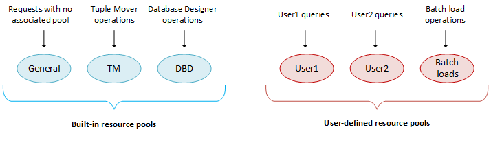
18.6.2.1 - Defining secondary resource pools
You can define secondary resource pools to which running queries can cascade if they exceed their primary pool's RUNTIMECAP .
You can define secondary resource pools to which running queries can cascade if they exceed their primary pool's RUNTIMECAP .
Identifying a secondary pool
Secondary resource pools designate a place where queries that exceed the RUNTIMECAP of the pool on which they are running can continue execution. If a query exceeds a pool's RUNTIMECAP, the query can cascade to a pool with a larger RUNTIMECAP instead of returning with an error. When a query cascades to another pool, the original pool regains the memory used by that query.
Unlike a user's primary resource pool, which requires USAGE privileges, Vertica does not check for user privileges on secondary resource pools. Thus, a user whose query cascades to a secondary resource pool requires no USAGE privileges on that resource pool.
You can define a secondary pool so it queues long-running queries if the pool lacks sufficient memory to handle that query immediately, by setting two parameters:
Eon Mode restrictions
In Eon Mode, you can associate user-defined resource pools with a subcluster. The following restrictions apply:
-
Global resource pools can cascade only to other global resource pools.
-
A subcluster resource pool can cascade to a global resource pool, or to another subcluster-specific resource pool that belongs to the same subcluster. If a subcluster-specific resource pool cascades to a user-defined resource pool that exists on both the global and subcluster level, the subcluster-level resource pool has priority. For example:
=> CREATE RESOURCE POOL billing1;
=> CREATE RESOURCE POOL billing1 FOR CURRENT SUBCLUSTER;
=> CREATE RESOURCE POOL billing2 FOR CURRENT SUBCLUSTER CASCADE TO billing1;
WARNING 9613: Resource pool billing1 both exists at both subcluster level and global level, assuming subcluster level
CREATE RESOURCE POOL
Query cascade path
Vertica routes queries to a secondary pool when the RUNTIMECAP on an initial pool is reached. Vertica then checks the secondary pool's RUNTIMECAP value. If the secondary pool's RUNTIMECAP is greater than the initial pool's value, the query executes on the secondary pool. If the secondary pool's RUNTIMECAP is less than or equal to the initial pool's value, Vertica retries the query on the next pool in the chain until it finds a pool on which the RUNTIMECAP is greater than the initial pool's value. If the secondary pool does not have sufficient resources available to execute the query at that time, SELECT queries may re-queue, re-plan, and abort on that pool. Other types of queries will fail due to insufficient resources. If no appropriate secondary pool exists for a query, the query will error out.
The following diagram demonstrates the path a query takes to execution.
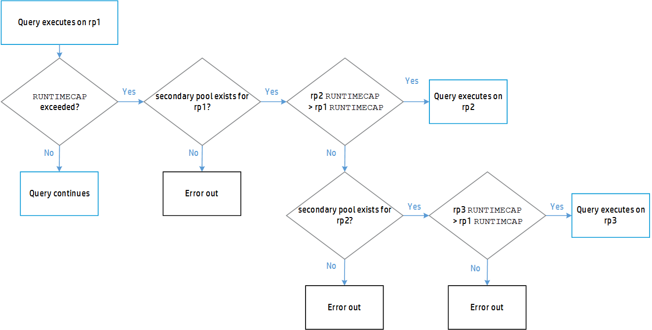
Query execution time allocation
After Vertica finds an appropriate pool on which to run the query, it continues to execute that query uninterrupted. The query now has the difference of the two pools' RUNTIMECAP limits in which to complete:
query execution time allocation = rp2 RUNTIMECAP - rp1 RUNTIMECAP
Using CASCADE TO
As a superuser, you can identify an existing resource pool—either user-defined pool or the GENERAL pool—by using the CASCADE TO parameter in the CREATE RESOURCE POOL or ALTER RESOURCE POOL statement.
In the following example, two resource pools are created and associated with a user as follows:
- The
shortUserQueries resource pool is created with a one-minute RUNTIMECAP
- The
userOverflow resource pool is created with a RUNTIMECAP of five minutes.
shortUserQueries is modified with ALTER RESOURCE POOL...CASCADE to use userOverflow to handle queries that require more than one minute to process.- The user
molly is created and configured to use shortUserQueries to handle that user's queries.
Given this scenario, queries issued by molly are initially directed to shortUserQueries for handling; queries that require more than one minute of processing time automatically cascade to the userOverflow pool to complete execution. Using the secondary pool frees up space in the primary pool, which is configured to handle short queries:
=> CREATE RESOURCE POOL shortUserQueries RUNTIMECAP '1 minutes'
=> CREATE RESOURCE POOL userOverflow RUNTIMECAP '5 minutes';
=> ALTER RESOURCE POOL shortUserQueries CASCADE TO userOverflow;
=> CREATE USER molly RESOURCE POOL shortUserQueries;
If desired, you can modify this scenario so userOverflow can queue long-running queries until it is available to handle them, by setting the PRIORITY and QUEUETIMEOUT parameters:
=> ALTER RESOURCE POOL userOverflow PRIORITY HOLD QUEUETIMEOUT '10 minutes';
In this scenario, a query that cascades to userOverflow can be queued up to 10 minutes until userOverflow acquires the memory it requires to handle it. After 10 minutes elapse, the query is rejected and returns with an error.
Dropping a secondary pool
If you try to drop a resource pool that is the secondary pool for another resource pool, Vertica returns an error. The error lists the resource pools that depend on the secondary pool you tried to drop. To drop a secondary resource pool, first set the CASCADE TO parameter to DEFAULT on the primary resource pool, and then drop the secondary pool.
For example, you can drop resource pool rp2, which is a secondary pool for rp1, as follows:
=> ALTER RESOURCE POOL rp1 CASCADE TO DEFAULT;
=> DROP RESOURCE POOL rp2;
Secondary pool parameter dependencies
In general, a secondary pool's parameters are applied to an incoming query. In the case of RUNTIMEPRIORITY , the following dependencies apply:
-
If the RUNTIMEPRIORITYTHRESHOLD timer was not started when the query was running in the primary pool, the query adopts the secondary resource pools' RUNTIMEPRIORITY when it cascades. This happens either when the RUNTIMEPRIORITYTHRESHOLD is not set for the primary pool or the RUNTIMEPRIORITY is set to HIGH for the primary pool.
-
If the RUNTIMEPRIORITYTHRESHOLD was reached in the primary pool, the query adopts the secondary resource pools' RUNTIMEPRIORITY when it cascades.
-
If the RUNTIMEPRIORITYTHRESHOLD was not reached in the primary pool and the secondary pool has no threshold, the query adopts the new pool's RUNTIMEPRIORITY when it cascades.
-
If the RUNTIMEPRIORITYTHRESHOLD was not reached in the primary pool and the secondary pool has a threshold set.
-
If the primary pool's RUNTIMEPRIORITYTHRESHOLD is greater than or equal to the secondary pool's RUNTIMEPRIORITYTHRESHOLD , the query adopts the secondary pool's RUNTIMEPRIORITY after the query reaches the RUNTIMEPRIORITYTHRESHOLD of the primary pool.
For example:
RUNTIMECAP of primary pool = 5 sec
RUNTIMEPRIORITYTHRESHOLD of primary pool = 8 sec
RUNTIMTPRIORITYTHRESHOLD of secondary pool = 7 sec
In this case, the query runs for 5 seconds on the primary pool and then cascades to the secondary pool. After another 3 seconds, 8 seconds total, the query adopts the RUNTIMEPRIORITY of the secondary pool.
-
If the primary pool's RUNTIMEPRIORITYTHRESHOLD is less than the secondary pool's RUNTIMEPRIORITYTHRESHOLD, the query adopts the secondary pool's RUNTIMEPRIORITY after the query reaches the RUNTIMEPRIORITYTHRESHOLD of the secondary pool.
In this case, the query runs for 5 seconds on the primary pool and then cascades to the secondary pool. After another 7 seconds, 12 seconds total, the query adopts the RUNTIMEPRIORITY of the secondary pool.:
RUNTIMECAP of primary pool = 5 sec
RUNTIMEPRIORITYTHRESHOLD of primary pool = 8 sec
RUNTIMTPRIORITYTHRESHOLD of secondary pool = 12 se
CASCADE errors
A query that cascades to a secondary resource pool typically returns with an error in the following cases:
* The resource pool cannot acquire the memory it needs to finish processing the query.
* The secondary resource pool parameter [MAXCONCURRENCY ](/en/sql-reference/statements/create-statements/create-resource-pool/#MAXCONCURRENCY)is set to 1 and it is already processing another query.
18.6.2.2 - Querying resource pool settings
You can use the following to get information about resource pools:.
You can use the following to get information about resource pools:
-
RESOURCE_POOLS returns resource pool settings from the Vertica database catalog, as set by
CREATE RESOURCE POOL and
ALTER RESOURCE POOL.
-
SUBCLUSTER_RESOURCE_POOL_OVERRIDES displays all subcluster level overrides of global resource pool settings.
For runtime information about resource pools, see Monitoring resource pools.
Querying resource pool settings
The following example queries various settings of two internal resource pools, GENERAL and TM:
=> SELECT name, subcluster_oid, subcluster_name, maxmemorysize, memorysize, runtimepriority, runtimeprioritythreshold, queuetimeout
FROM RESOURCE_POOLS WHERE name IN('general', 'tm');
name | subcluster_oid | subcluster_name | maxmemorysize | memorysize | runtimepriority | runtimeprioritythreshold | queuetimeout
---------+----------------+-----------------+---------------+------------+-----------------+--------------------------+--------------
general | 0 | | Special: 95% | | MEDIUM | 2 | 00:05
tm | 0 | | | 3G | MEDIUM | 60 | 00:05
(2 rows)
Viewing overrides to global resource pools
In Eon Mode, you can query SUBCLUSTER_RESOURCE_POOL_OVERRIDES in the system tables to view any overrides to global resource pools for individual subclusters. The following query shows an override that sets MEMORYSIZE and MAXMEMORYSIZE for the built-in resource pool TM to 0% in the analytics_1 subcluster. These settings prevent the subcluster from performing Tuple Mover mergeout tasks.
=> SELECT * FROM SUBCLUSTER_RESOURCE_POOL_OVERRIDES;
pool_oid | name | subcluster_oid | subcluster_name | memorysize | maxmemorysize | maxquerymemorysize
-------------------+------+-------------------+-----------------+------------+---------------+--------------------
45035996273705058 | tm | 45035996273843504 | analytics_1 | 0% | 0% |
(1 row)
18.6.2.3 - User profiles
User profiles are attributes associated with a user that control that user's access to several system resources.
User profiles are attributes associated with a user that control that user's access to several system resources. These resources include:
-
Resource pool to which a user is assigned (RESOURCE POOL)
-
Maximum amount of memory a user's session can use (MEMORYCAP)
-
Maximum amount of temporary file storage a user's session can use (TEMPSPACECAP)
-
Maximum amount of time a user's query can run (RUNTIMECAP)
You can set these attributes with the CREATE USER statement and modify the attributes later with ALTER USER.
Two strategies limit a user's access to resources: setting attributes on the user directly to control resource use, or assigning the user to a resource pool. The first method lets you fine tune individual users, while the second makes it easier to group many users together and set their collective resource usage.
If you limit user resources collectively with resource pool assignments, consider the following:
-
A user cannot log in to Vertica unless they either have privileges to the GENERAL pool, or are assigned to a default resource pool.
-
If a user's default resource pool is dropped, the user's queries use the GENERAL pool.
-
If a user does not have privileges to the GENERAL pool and you attempt to drop their assigned resource pool, the DROP operation fails.
In an Eon Mode database, you can set the user's default resource pool to a subcluster-specific resource pool. If that is the case, Vertica uses one of the following methods to determine which resource pool is used for queries when a user connects to a subcluster:
-
If the subcluster uses their assigned default resource pool, then the user's queries use their assigned resource pool.
-
If the subcluster does not use their assigned default resource pool, but the user has access to the GENERAL pool, the user's queries use the GENERAL pool.
-
If the subcluster does not use the resource pool assigned to the user, and the user does not have privileges to the GENERAL pool, then the user cannot query from any node of this subcluster.
The following examples illustrate how to set a user's resource pool attributes. For additional examples, see the scenarios described in Using user-defined pools and user-profiles for workload management.
Example
Set the user's RESOURCE POOL attribute to assign the user to a resource pool. To create a user named user1 who has access to the resource pool my_pool, use the command:
=> CREATE USER user1 RESOURCE POOL my_pool;
To limit the amount of memory for a user without designating a pool, set the user's MEMORYCAP to either a particular unit or a percentage of the total memory available. For example, to create a user named user2 whose sessions are limited to using 200 MBs memory each, use the command:
=> CREATE USER user2 MEMORYCAP '200M';
To limit the time a user's queries are allowed to run, set the RUNTIMECAP attribute. To prevent queries for user2 from running more than five minutes, use this command:
=> ALTER USER user2 RUNTIMECAP '5 minutes';
To limit the amount of temporary disk space that the user's sessions can use, set the TEMPSPACECAP to either a particular size or a percentage of temporary disk space available. For example, the next statement creates user3, and limits her to using 1 GB of temporary space:
=> CREATE USER user3 TEMPSPACECAP '1G';
You can combine different attributes into a single command. For example, to limit the MEMORYCAP and RUNTIMECAP for user3, include both attributes in an ALTER USER statement:
=> ALTER USER user3 MEMORYCAP '750M' RUNTIMECAP '10 minutes';
ALTER USER
=> \x
Expanded display is on.
=> SELECT * FROM USERS;
-[ RECORD 1 ]-----+------------------
user_id | 45035996273704962
user_name | release
is_super_user | t
resource_pool | general
memory_cap_kb | unlimited
temp_space_cap_kb | unlimited
run_time_cap | unlimited
-[ RECORD 2 ]-----+------------------
user_id | 45035996273964824
user_name | user1
is_super_user | f
resource_pool | my_pool
memory_cap_kb | unlimited
temp_space_cap_kb | unlimited
run_time_cap | unlimited
-[ RECORD 3 ]-----+------------------
user_id | 45035996273964832
user_name | user2
is_super_user | f
resource_pool | general
memory_cap_kb | 204800
temp_space_cap_kb | unlimited
run_time_cap | 00:05
-[ RECORD 4 ]-----+------------------
user_id | 45035996273970230
user_name | user3
is_super_user | f
resource_pool | general
memory_cap_kb | 768000
temp_space_cap_kb | 1048576
run_time_cap | 00:10
See also
18.6.2.4 - Query budgeting
Before it can execute a query, Vertica devises a query plan, which it sends to each node that will participate in executing the query.
Before it can execute a query, Vertica devises a query plan, which it sends to each node that will participate in executing the query. The Resource Manager evaluates the plan on each node and estimates how much memory and concurrency the node needs to execute its part of the query. This is the query budget, which Vertica stores in the query_budget_kb column of system table
V_MONITOR.RESOURCE_POOL_STATUS.
A query budget is based on several parameter settings of the resource pool where the query will execute:
-
MEMORYSIZE
-
MAXMEMORYSIZE
-
PLANNEDCONCURRENCY
You can modify MAXMEMORYSIZE and PLANNEDCONCURRENCY for the GENERAL resource pool with
ALTER RESOURCE POOL. This resource pool typically executes queries that are not assigned to a user-defined resource pool. You can set all three parameters for any user-defined resource pool when you create it with
CREATE RESOURCE POOL, or later with
ALTER RESOURCE POOL.
Important
You can also limit how much memory that a pool can allocate at runtime to its queries, by setting parameter
MAXQUERYMEMORYSIZE on that pool. For more information, see
CREATE RESOURCE POOL.
Computing the GENERAL pool query budget
Vertica calculates query budgets in the GENERAL pool with the following formula:
queryBudget = queuingThresholdPool / PLANNEDCONCURRENCY
Note
Vertica calculates the GENERAL pool's queuing threshold as 95 percent of its MAXMEMORYSIZE setting.
Computing query budgets for user-defined resource pools
For user-defined resource pools, Vertica uses the following algorithm:
-
If MEMORYSIZE is set to 0 and MAXMEMORYSIZE is not set:
queryBudget = queuingThresholdGeneralPool / PLANNEDCONCURRENCY
-
If MEMORYSIZE is set to 0 and MAXMEMORYSIZE is set to a non-default value:
query-budget = queuingThreshold / PLANNEDCONCURRENCY
Note
Vertica calculates a user-defined pool's queuing threshold as 95 percent of its MAXMEMORYSIZE setting.
-
If MEMORYSIZE is set to a non-default value:
queryBudget = MEMORYSIZE / PLANNEDCONCURRENCY
By carefully tuning a resource pool's MEMORYSIZE and PLANNEDCONCURRENCY parameters, you can control how much memory can be budgeted for queries.
Caution
Query budgets do not typically require tuning, However, if you reduce the MAXMEMORYSIZE because you need memory for other purposes, be aware that doing so also reduces the query budget. Reducing the query budget negatively impacts the query performance, particularly if the queries are complex.
To maintain the original query budget for the resource pool, be sure to reduce parameters MAXMEMORYSIZE and PLANNEDCONCURRENCY together.
See also
Do You Need to Put Your Query on a Budget? in the Vertica User Community.
18.6.3 - Managing resources at query run time
The Resource Manager estimates the resources required for queries to run, and then prioritizes them.
The Resource Manager estimates the resources required for queries to run, and then prioritizes them. You can control how the Resource Manager prioritizes query execution in several ways:
18.6.3.1 - Setting runtime priority for the resource pool
For each resource pool, you can manage resources that are assigned to queries that are already running.
For each resource pool, you can manage resources that are assigned to queries that are already running. You assign each resource pool a runtime priority of HIGH, MEDIUM, or LOW. These settings determine the amount of runtime resources (such as CPU and I/O bandwidth) assigned to queries in the resource pool when they run. Queries in a resource pool with a HIGH priority are assigned greater runtime resources than those in resource pools with MEDIUM or LOW runtime priorities.
Prioritizing queries within a resource pool
While runtime priority helps to manage resources for the resource pool, there may be instances where you want some flexibility within a resource pool. For instance, you may want to ensure that very short queries run at a high priority, while also ensuring that all other queries run at a medium or low priority.
The Resource Manager allows you this flexibility by letting you set a runtime priority threshold for the resource pool. With this threshold, you specify a time limit (in seconds) by which a query must finish before it is assigned the runtime priority of the resource pool. All queries begin running with a HIGH priority; once a query's duration exceeds the time limit specified in the runtime priority threshold, it is assigned the runtime priority of the resource pool.
Setting runtime priority and runtime priority threshold
You specify runtime priority and runtime priority threshold by setting two resource pool parameters with
CREATE RESOURCE POOL or
ALTER RESOURCE POOL:
-
RUNTIMEPRIORITY
-
RUNTIMEPRIORITYTHRESHOLD
18.6.3.2 - Changing runtime priority of a running query
CHANGE_CURRENT_STATEMENT_RUNTIME_PRIORITY lets you to change a query's runtime priority.
CHANGE_CURRENT_STATEMENT_RUNTIME_PRIORITY lets you to change a query's runtime priority. You can change the runtime priority of a query that is already executing.
This function takes two arguments:
-
The query's transaction ID, obtained from the system table
SESSIONS
-
The desired priority, one of the following string values: HIGH, MEDIUM, or LOW
Restrictions
Superusers can change the runtime priority of any query to any priority level. The following restrictions apply to other users:
Procedure
Changing a query's runtime priority is a two-step procedure:
-
Get the query's transaction ID by querying the system table
SESSIONS. For example, the following statement returns information about all running queries:
=> SELECT transaction_id, runtime_priority, transaction_description from SESSIONS;
-
Run `CHANGE_CURRENT_STATEMENT_RUNTIME_PRIORITY```, specifying the query's transaction ID and desired runtime priority:
=> SELECT CHANGE_CURRENT_STATEMENT_RUNTIME_PRIORITY(45035996273705748, 'low')
18.6.3.3 - Manually moving queries to different resource pools
If you are the database administrator, you can move queries to another resource pool mid-execution using the MOVE_STATEMENT_TO_RESOURCE_POOL meta-function.
If you are the database administrator, you can move queries to another resource pool mid-execution using the MOVE_STATEMENT_TO_RESOURCE_POOL meta-function.
You might want to use this feature if a single query is using a large amount of resources, preventing smaller queries from executing.
What happens when a query moves to a different resource pool
When a query is moved from one resource pool to another, it continues executing, provided the target pool has enough resources to accommodate the incoming query. If sufficient resources cannot be assigned in the target pool on at least one node, Vertica cancels the query and attempts to re-plan the query. If Vertica cannot re-plan the query, the query is canceled indefinitely.
When you successfully move a query to a target resource pool, its resources will be accounted for by the target pool and released on the first pool.
If you move a query to a resource pool with PRIORITY HOLD, Vertica cancels the query and queues it on the target pool. This cancellation remains in effect until you change the PRIORITY or move the query to another pool without PRIORITY HOLD. You can use this option if you want to store long-running queries for later use.
You can view the RESOURCE_ACQUISITIONS or RESOURCE_POOL_STATUS system tables to determine if the target pool can accommodate the query you want to move. Be aware that the system tables may change between the time you query the tables and the time you invoke the MOVE_STATEMENT_TO_RESOURCE_POOL meta-function.
When a query successfully moves from one resource pool to another mid-execution, it executes until the greater of the existing and new RUNTIMECAP is reached. For example, if the RUNTIMECAP on the initial pool is greater than that on the target pool, the query can execute until the initial RUNTIMECAP is reached.
When a query successfully moves from one resource pool to another mid-execution the CPU affinity will change.
Using the MOVE_STATEMENT_TO_RESOURCE_POOL function
To manually move a query from its current resource pool to another resource pool, use the MOVE_STATEMENT_TO_RESOURCE_POOL meta-function. Provide the session id, transaction id, statement id, and target resource pool name, as shown:
=> SELECT MOVE_STATEMENT_TO_RESOURCE_POOL ('v_vmart_node0001.example.-31427:0x82fbm', 45035996273711993, 1, 'my_target_pool');
See also:
18.6.4 - Restoring resource manager defaults
System table RESOURCE_POOL_DEFAULTS stores default values for all parameters for all built-in and user-defined resource pools.
System table RESOURCE_POOL_DEFAULTS stores default values for all parameters for all built-in and user-defined resource pools.
If you have changed the value of any parameter in any of your resource pools and want to restore it to its default, you can simply alter the table and set the parameter to DEFAULT. For example, the following statement sets the RUNTIMEPRIORITY for the resource pool sysquery back to its default value:
=> ALTER RESOURCE POOL sysquery RUNTIMEPRIORITY DEFAULT;
18.6.5 - Best practices for managing workload resources
This section provides general guidelines and best practices on how to set up and tune resource pools for various common scenarios.
This section provides general guidelines and best practices on how to set up and tune resource pools for various common scenarios.
Note
The exact settings for resource pool parameters are heavily dependent on your query mix, data size, hardware configuration, and concurrency requirements. Vertica recommends performing your own experiments to determine the optimal configuration for your system.
18.6.5.1 - Basic principles for scalability and concurrency tuning
A Vertica database runs on a cluster of commodity hardware.
A Vertica database runs on a cluster of commodity hardware. All loads and queries running against the database take up system resources, such as CPU, memory, disk I/O bandwidth, file handles, and so forth. The performance (run time) of a given query depends on how much resource it has been allocated.
When running more than one query concurrently on the system, both queries are sharing the resources; therefore, each query could take longer to run than if it was running by itself. In an efficient and scalable system, if a query takes up all the resources on the machine and runs in X time, then running two such queries would double the run time of each query to 2X. If the query runs in > 2X, the system is not linearly scalable, and if the query runs in < 2X then the single query was wasteful in its use of resources. Note that the above is true as long as the query obtains the minimum resources necessary for it to run and is limited by CPU cycles. Instead, if the system becomes bottlenecked so the query does not get enough of a particular resource to run, then the system has reached a limit. In order to increase concurrency in such cases, the system must be expanded by adding more of that resource.
In practice, Vertica should achieve near linear scalability in run times, with increasing concurrency, until a system resource limit is reached. When adequate concurrency is reached without hitting bottlenecks, then the system can be considered as ideally sized for the workload.
Note
Typically Vertica queries on segmented tables run on multiple (likely all) nodes of the cluster. Adding more nodes generally improves the run time of the query almost linearly.
18.6.5.2 - Setting a runtime limit for queries
You can set a limit for the amount of time a query is allowed to run.
You can set a limit for the amount of time a query is allowed to run. You can set this limit at three levels, listed in descending order of precedence:
-
The resource pool to which the user is assigned.
-
User profile with RUNTIMECAP configuredby
CREATE USER/
ALTER USER
-
Session queries, set by
SET SESSION RUNTIMECAP
In all cases, you set the runtime limit with an interval value that does not exceed one year. When you set runtime limit at multiple levels, Vertica always uses the shortest value. If a runtime limit is set for a non-superuser, that user cannot set any session to a longer runtime limit. Superusers can set the runtime limit for other users and for their own sessions, to any value up to one year, inclusive.
Example
user1 is assigned to the ad_hoc_queries resource pool:
=> CREATE USER user1 RESOURCE POOL ad_hoc_queries;
RUNTIMECAP for user1 is set to 1 hour:
=> ALTER USER user1 RUNTIMECAP '60 minutes';
RUNTIMECAP for the ad_hoc_queries resource pool is set to 30 minutes:
=> ALTER RESOURCE POOL ad_hoc_queries RUNTIMECAP '30 minutes';
In this example, Vertica terminates user1's queries if they exceed 30 minutes. Although the user1's runtime limit is set to one hour, the pool on which the query runs, which has a 30-minute runtime limit, has precedence.
Note
If a secondary pool for the ad_hoc_queries pool is specified using the CASCADE TO function, the query executes on that pool when the RUNTIMECAP on the ad_hoc_queries pool is surpassed.
See also
18.6.5.3 - Handling session socket blocking
A session socket can be blocked while awaiting client input or output for a given query.
A session socket can be blocked while awaiting client input or output for a given query. Session sockets are typically blocked for numerous reasons—for example, when the Vertica execution engine transmits data to the client, or a
COPY LOCAL operation awaits load data from the client.
In rare cases, a session socket can remain indefinitely blocked. For example, a query times out on the client, which tries to forcibly cancel the query, or relies on the session RUNTIMECAP setting to terminate it. In either case, if the query ends while awaiting messages or data, the socket can remain blocked and the session hang until it is forcibly closed.
Configuring a grace period
You can configure the system with a grace period, during which a lagging client or server can catch up and deliver a pending response. If the socket is blocked for a continuous period that exceeds the grace period setting, the server shuts down the socket and throws a fatal error. The session is then terminated. If no grace period is set, the query can maintain its block on the socket indefinitely.
You should set the session grace period high enough to cover an acceptable range of latency and avoid closing sessions prematurely—for example, normal client-side delays in responding to the server. Very large load operations might require you to adjust the session grace period as needed.
You can set the grace period at four levels, listed in descending order of precedence:
-
Session (highest)
-
User
-
Node
-
Database
Setting grace periods for the database and nodes
At the database and node levels, you set the grace period to any interval up to 20 days, through configuration parameter BlockedSocketGracePeriod:
-
ALTER DATABASE db-name SET BlockedSocketGracePeriod = 'interval';
-
ALTER NODE node-name SET BlockedSocketGracePeriod = 'interval';
By default, the grace period for both levels is set to an empty string, which allows unlimited blocking.
Setting grace periods for users and sessions
You can set the grace period for individual users and for a given session, as follows:
A user can set a session to any interval equal to or less than the grace period set for that user. Superusers can set the grace period for other users, and for their own sessions, to any value up to 20 days, inclusive.
Examples
Superuser dbadmin sets the database grace period to 6 hours. This limit only applies to non-superusers. dbadmin can sets the session grace period for herself to any value up to 20 days—in this case, 10 hours:
=> ALTER DATABASE VMart SET BlockedSocketGracePeriod = '6 hours';
ALTER DATABASE
=> SHOW CURRENT BlockedSocketGracePeriod;
level | name | setting
----------+--------------------------+---------
DATABASE | BlockedSocketGracePeriod | 6 hours
(1 row)
=> SET SESSION GRACEPERIOD '10 hours';
SET
=> SHOW GRACEPERIOD;
name | setting
-------------+---------
graceperiod | 10:00
(1 row)
dbadmin creates user user777 created with no grace period setting. Thus, the effective grace period for user777 is derived from the database setting of BlockedSocketGracePeriod, which is 6 hours. Any attempt by user777 to set the session grace period to a value greater than 6 hours returns with an error:
=> CREATE USER user777;
=> \c - user777
You are now connected as user "user777".
=> SHOW GRACEPERIOD;
name | setting
-------------+---------
graceperiod | 06:00
(1 row)
=> SET SESSION GRACEPERIOD '7 hours';
ERROR 8175: The new period 07:00 would exceed the database limit of 06:00
dbadmin sets a grace period of 5 minutes for user777. Now, user777 can set the session grace period to any value equal to or less than the user-level setting:
=> \c
You are now connected as user "dbadmin".
=> ALTER USER user777 GRACEPERIOD '5 minutes';
ALTER USER
=> \c - user777
You are now connected as user "user777".
=> SET SESSION GRACEPERIOD '6 minutes';
ERROR 8175: The new period 00:06 would exceed the user limit of 00:05
=> SET SESSION GRACEPERIOD '4 minutes';
SET
18.6.5.4 - Using user-defined pools and user-profiles for workload management
The scenarios in this section describe common workload-management issues, and provide solutions with examples.
The scenarios in this section describe common workload-management issues, and provide solutions with examples.
18.6.5.4.1 - Periodic batch loads
You do batch loads every night, or occasionally (infrequently) during the day.
Scenario
You do batch loads every night, or occasionally (infrequently) during the day. When loads are running, it is acceptable to reduce resource usage by queries, but at all other times you want all resources to be available to queries.
Solution
Create a separate resource pool for loads with a higher priority than the preconfigured setting on the build-in GENERAL pool.
In this scenario, nightly loads get preference when borrowing memory from the GENERAL pool. When loads are not running, all memory is automatically available for queries.
Example
Create a resource pool that has higher priority than the GENERAL pool:
-
Create resource pool load_pool with PRIORITY set to 10:
=> CREATE RESOURCE POOL load_pool PRIORITY 10;
-
Modify user load_user to use the new resource pool:
=> ALTER USER load_user RESOURCE POOL load_pool;
18.6.5.4.2 - CEO query
The CEO runs a report every Monday at 9AM, and you want to be sure that the report always runs.
Scenario
The CEO runs a report every Monday at 9AM, and you want to be sure that the report always runs.
Solution
To ensure that a certain query or class of queries always gets resources, you could create a dedicated pool for it as follows:
-
Using the PROFILE command, run the query that the CEO runs every week to determine how much memory should be allocated:
=> PROFILE SELECT DISTINCT s.product_key, p.product_description
-> FROM store.store_sales_fact s, public.product_dimension p
-> WHERE s.product_key = p.product_key AND s.product_version = p.product_version
-> AND s.store_key IN (
-> SELECT store_key FROM store.store_dimension
-> WHERE store_state = 'MA')
-> ORDER BY s.product_key;
-
At the end of the query, the system returns a notice with resource usage:
NOTICE: Statement is being profiled.HINT: select * from v_monitor.execution_engine_profiles where
transaction_id=45035996273751349 and statement_id=6;
NOTICE: Initiator memory estimate for query: [on pool general: 1723648 KB,
minimum: 355920 KB]
-
Create a resource pool with MEMORYSIZE reported by the above hint to ensure that the CEO query has at least this memory reserved for it:
=> CREATE RESOURCE POOL ceo_pool MEMORYSIZE '1800M' PRIORITY 10;
CREATE RESOURCE POOL
=> \x
Expanded display is on.
=> SELECT * FROM resource_pools WHERE name = 'ceo_pool';
-[ RECORD 1 ]-------+-------------
name | ceo_pool
is_internal | f
memorysize | 1800M
maxmemorysize |
priority | 10
queuetimeout | 300
plannedconcurrency | 4
maxconcurrency |
singleinitiator | f
-
Assuming the CEO report user already exists, associate this user with the above resource pool using ALTER USER statement.
=> ALTER USER ceo_user RESOURCE POOL ceo_pool;
-
Issue the following command to confirm that the ceo_user is associated with the ceo_pool:
=> SELECT * FROM users WHERE user_name ='ceo_user';
-[ RECORD 1 ]-+------------------
user_id | 45035996273713548
user_name | ceo_user
is_super_user | f
resource_pool | ceo_pool
memory_cap_kb | unlimited
If the CEO query memory usage is too large, you can ask the Resource Manager to reduce it to fit within a certain budget. See Query budgeting.
18.6.5.4.3 - Preventing runaway queries
Joe, a business analyst often runs big reports in the middle of the day that take up the whole machine's resources.You want to prevent Joe from using more than 100MB of memory, and you want to also limit Joe's queries to run for less than 2 hours.
Scenario
Joe, a business analyst often runs big reports in the middle of the day that take up the whole machine's resources.You want to prevent Joe from using more than 100MB of memory, and you want to also limit Joe's queries to run for less than 2 hours.
Solution
User profiles provides a solution to this scenario. To restrict the amount of memory Joe can use at one time, set a MEMORYCAP for Joe to 100MB using the ALTER USER command. To limit the amount of time that Joe's query can run, set a RUNTIMECAP to 2 hours using the same command. If any query run by Joe takes up more than its cap, Vertica rejects the query.
If you have a whole class of users whose queries you need to limit, you can also create a resource pool for them and set RUNTIMECAP for the resource pool. When you move these users to the resource pool, Vertica limits all queries for these users to the RUNTIMECAP you specified for the resource pool.
Example
=> ALTER USER analyst_user MEMORYCAP '100M' RUNTIMECAP '2 hours';
If Joe attempts to run a query that exceeds 100MB, the system returns an error that the request exceeds the memory session limit, such as the following example:
\i vmart_query_04.sqlvsql:vmart_query_04.sql:12: ERROR: Insufficient resources to initiate plan
on pool general [Request exceeds memory session limit: 137669KB > 102400KB]
Only the system database administrator (dbadmin) can increase only the MEMORYCAP setting. Users cannot increase their own MEMORYCAP settings and will see an error like the following if they attempt to edit their MEMORYCAP or RUNTIMECAP settings:
ALTER USER analyst_user MEMORYCAP '135M';
ROLLBACK: permission denied
18.6.5.4.4 - Restricting resource usage of ad hoc query application
You recently made your data warehouse available to a large group of users who are inexperienced with SQL.
Scenario
You recently made your data warehouse available to a large group of users who are inexperienced with SQL. Some users run reports that operate on a large number of rows and overwhelm the system. You want to throttle system usage by these users.
Solution
-
Create a resource pool for ad hoc applications where MAXMEMORYSIZE is equal to MEMORYSIZE. This prevents queries in that resource pool from borrowing resources from the GENERAL pool. Also, set RUNTIMECAP to limit the maximum duration of ad hoc queries:
=> CREATE RESOURCE POOL adhoc_pool
MEMORYSIZE '200M'
MAXMEMORYSIZE '200M'
RUNTIMECAP '20 seconds'
PRIORITY 0
QUEUETIMEOUT 300
PLANNEDCONCURRENCY 4;
=> SELECT pool_name, memory_size_kb, queueing_threshold_kb
FROM V_MONITOR.RESOURCE_POOL_STATUS WHERE pool_name='adhoc_pool';
pool_name | memory_size_kb | queueing_threshold_kb
------------+----------------+-----------------------
adhoc_pool | 204800 | 153600
(1 row)
-
Associate this resource pool with database users who use the application to connect to the database.
=> ALTER USER app1_user RESOURCE POOL adhoc_pool;
18.6.5.4.5 - Setting a hard limit on concurrency for an application
For billing purposes, analyst Jane would like to impose a hard limit on concurrency for this application.
Scenario
For billing purposes, analyst Jane would like to impose a hard limit on concurrency for this application. How can she achieve this?
Solution
The simplest solution is to create a separate resource pool for the users of that application and set its MAXCONCURRENCY to the desired concurrency level. Any queries beyond MAXCONCURRENCY are queued.
Tip
Vertica recommends leaving PLANNEDCONCURRENCY to the default level so the queries get their maximum amount of resources. The system as a whole thus runs with the highest efficiency.
Example
In this example, there are four billing users associated with the billing pool. The objective is to set a hard limit on the resource pool so a maximum of three concurrent queries can be executed at one time. All other queries will queue and complete as resources are freed.
=> CREATE RESOURCE POOL billing_pool MAXCONCURRENCY 3 QUEUETIMEOUT 2;
=> CREATE USER bill1_user RESOURCE POOL billing_pool;
=> CREATE USER bill2_user RESOURCE POOL billing_pool;
=> CREATE USER bill3_user RESOURCE POOL billing_pool;
=> CREATE USER bill4_user RESOURCE POOL billing_pool;
=> \x
Expanded display is on.
=> select maxconcurrency,queuetimeout from resource_pools where name = 'billing_pool';
maxconcurrency | queuetimeout
----------------+--------------
3 | 2
(1 row)
> SELECT reason, resource_type, rejection_count FROM RESOURCE_REJECTIONS
WHERE pool_name = 'billing_pool' AND node_name ilike '%node0001';
reason | resource_type | rejection_count
---------------------------------------+---------------+-----------------
Timedout waiting for resource request | Queries | 16
(1 row)
If queries are running and do not complete in the allotted time (default timeout setting is 5 minutes), the next query requested gets an error similar to the following:
ERROR: Insufficient resources to initiate plan on pool billing_pool [Timedout waiting for resource request: Request exceeds limits:
Queries Exceeded: Requested = 1, Free = 0 (Limit = 3, Used = 3)]
The table below shows that there are three active queries on the billing pool.
=> SELECT pool_name, thread_count, open_file_handle_count, memory_inuse_kb FROM RESOURCE_ACQUISITIONS
WHERE pool_name = 'billing_pool';
pool_name | thread_count | open_file_handle_count | memory_inuse_kb
--------------+--------------+------------------------+-----------------
billing_pool | 4 | 5 | 132870
billing_pool | 4 | 5 | 132870
billing_pool | 4 | 5 | 132870
(3 rows)
18.6.5.4.6 - Handling mixed workloads: batch versus interactive
You have a web application with an interactive portal.
Scenario
You have a web application with an interactive portal. Sometimes when IT is running batch reports, the web page takes a long time to refresh and users complain, so you want to provide a better experience to your web site users.
Solution
The principles learned from the previous scenarios can be applied to solve this problem. The basic idea is to segregate the queries into two groups associated with different resource pools. The prerequisite is that there are two distinct database users issuing the different types of queries. If this is not the case, do consider this a best practice for application design.
**Method 1
**Create a dedicated pool for the web page refresh queries where you:
-
Size the pool based on the average resource needs of the queries and expected number of concurrent queries issued from the portal.
-
Associate this pool with the database user that runs the web site queries. SeeCEO query for information about creating a dedicated pool.
This ensures that the web site queries always run and never queue behind the large batch jobs. Leave the batch jobs to run off the GENERAL pool.
For example, the following pool is based on the average resources needed for the queries running from the web and the expected number of concurrent queries. It also has a higher PRIORITY to the web queries over any running batch jobs and assumes the queries are being tuned to take 250M each:
=> CREATE RESOURCE POOL web_pool
MEMORYSIZE '250M'
MAXMEMORYSIZE NONE
PRIORITY 10
MAXCONCURRENCY 5
PLANNEDCONCURRENCY 1;
**Method 2
**Create a resource pool with fixed memory size. This limits the amount of memory available to batch reports so memory is always left over for other purposes. For details, see Restricting resource usage of ad hoc query application.
For example:
=> CREATE RESOURCE POOL batch_pool
MEMORYSIZE '4G'
MAXMEMORYSIZE '4G'
MAXCONCURRENCY 10;
The same principle can be applied if you have three or more distinct classes of workloads.
18.6.5.4.7 - Setting priorities on queries issued by different users
You want user queries from one department to have a higher priority than queries from another department.
Scenario
You want user queries from one department to have a higher priority than queries from another department.
Solution
The solution is similar to the mixed workload case. In this scenario, you do not limit resource usage; you set different priorities. To do so, create two different pools, each with MEMORYSIZE=0% and a different PRIORITY parameter. Both pools borrow from the GENERAL pool, however when competing for resources, the priority determine the order in which each pool's request is granted. For example:
=> CREATE RESOURCE POOL dept1_pool PRIORITY 5;
=> CREATE RESOURCE POOL dept2_pool PRIORITY 8;
If you find this solution to be insufficient, or if one department's queries continuously starves another department’s users, you can add a reservation for each pool by setting MEMORYSIZE so some memory is guaranteed to be available for each department.
For example, both resources use the GENERAL pool for memory, so you can allocate some memory to each resource pool by using ALTER RESOURCE POOL to change MEMORYSIZE for each pool:
=> ALTER RESOURCE POOL dept1_pool MEMORYSIZE '100M';
=> ALTER RESOURCE POOL dept2_pool MEMORYSIZE '150M';
18.6.5.4.8 - Continuous load and query
You want your application to run continuous load streams, but many have up concurrent query streams.
Scenario
You want your application to run continuous load streams, but many have up concurrent query streams. You want to ensure that performance is predictable.
Solution
The solution to this scenario depends on your query mix. In all cases, the following approach applies:
-
Determine the number of continuous load streams required. This may be related to the desired load rate if a single stream does not provide adequate throughput, or may be more directly related to the number of sources of data to load. Create a dedicated resource pool for the loads, and associate it with the database user that will perform them. See CREATE RESOURCE POOL for details.
In general, concurrency settings for the load pool should be less than the number of cores per node. Unless the source processes are slow, it is more efficient to dedicate more memory per load, and have additional loads queue. Adjust the load pool's QUEUETIMEOUT setting if queuing is expected.
-
Run the load workload for a while and observe whether the load performance is as expected. If the Tuple Mover is not tuned adequately to cover the load behavior, see Managing the tuple mover.
-
If there is more than one kind of query in the system—for example, some queries must be answered quickly for interactive users, while others are part of a batch reporting process—follow the guidelines in Handling mixed workloads: batch versus interactive.
-
Let the queries run and observe performance. If some classes of queries do not perform as desired, then you might need to tune the GENERAL pool as outlined in Restricting resource usage of ad hoc query application, or create more dedicated resource pools for those queries. For more information, see CEO query and Handling mixed workloads: batch versus interactive.
See the sections on Managing workloads and CREATE RESOURCE POOL for information on obtaining predictable results in mixed workload environments.
18.6.5.4.9 - Prioritizing short queries at run time
You recently created a resource pool for users who are inexperienced with SQL and who frequently run ad hoc reports.
Scenario
You recently created a resource pool for users who are inexperienced with SQL and who frequently run ad hoc reports. Until now, you managed resource allocation by creating a resource pool where MEMORYSIZE and MAXMEMORYSIZE are equal. This prevented queries in that resource pool from borrowing resources from the GENERAL pool. Now you want to manage resources at run time and prioritize short queries so they are never queued as a result of limited run-time resources.
Solution
For example:
=> ALTER RESOURCE POOL ad_hoc_pool RUNTIMEPRIORITY medium RUNTIMEPRIORITYTHRESHOLD 5;
Because RUNTIMEPRIORITYTHRESHOLD is set to 5, all queries in resource pool ad_hoc_pool that complete within 5 seconds run at high priority. Queries that exceeds 5 seconds drop down to the RUNTIMEPRIORITY assigned to the resource pool, MEDIUM.
18.6.5.4.10 - Dropping the runtime priority of long queries
You want most queries in a resource pool to run at a HIGH runtime priority; however, you'd like to be able to drop jobs longer than 1 hour to a lower priority.
Scenario
You want most queries in a resource pool to run at a HIGH runtime priority; however, you'd like to be able to drop jobs longer than 1 hour to a lower priority.
Solution
Set the RUNTIMEPRIORITY for the resource pool to LOW and set the RUNTIMEPRIORITYTHRESHOLD to a number that cuts off only the longest jobs.
Example
To ensure that all queries with a duration of more than 3600 seconds (1 hour) are assigned a low runtime priority, modify the resource pool as follows:
=> ALTER RESOURCE POOL ad_hoc_pool RUNTIMEPRIORITY low RUNTIMEPRIORITYTHRESHOLD 3600;
18.6.5.5 - Tuning built-in pools
The scenarios in this section describe how to tune built-in pools.
The scenarios in this section describe how to tune built-in pools.
18.6.5.5.1 - Restricting Vertica to take only 60% of memory
You have a single node application that embeds Vertica, and some portion of the RAM needs to be devoted to the application process.
Scenario
You have a single node application that embeds Vertica, and some portion of the RAM needs to be devoted to the application process. In this scenario, you want to limit Vertica to use only 60% of the available RAM.
Solution
Set the MAXMEMORYSIZE parameter of the GENERAL pool to the desired memory size. See Resource pool architecture for a discussion on resource limits.
18.6.5.5.2 - Tuning for recovery
You have a large database that contains a single large table with two projections, and with default settings, recovery is taking too long.
Scenario
You have a large database that contains a single large table with two projections, and with default settings, recovery is taking too long. You want to give recovery more memory to improve speed.
Solution
Set PLANNEDCONCURRENCY and MAXCONCURRENCY in the RECOVERY pool to 1, so recovery can take as much memory as possible from the GENERAL pool and run only one thread at once.
Caution
This setting can slow down other queries in your system.
18.6.5.5.3 - Tuning for refresh
When a operation is running, system performance is affected and user queries are rejected.
Scenario
When a refresh operation is running, system performance is affected and user queries are rejected. You want to reduce the memory usage of the refresh job.
Solution
Set MEMORYSIZE in the REFRESH pool to a fixed value. The Resource Manager then tunes the refresh query to only use this amount of memory.
Important
Remember to reset MEMORYSIZE in the REFRESH pool to 0% after the refresh operation completes, so memory can be used for other operations.
18.6.5.5.4 - Tuning tuple mover pool settings
During heavy load operations, you occasionally notice spikes in the number of ROS containers.
Scenario 1
During heavy load operations, you occasionally notice spikes in the number of ROS containers. You would like the Tuple Mover to perform mergeout more aggressively to consolidate ROS containers, and avoid ROS pushback.
Solution
Use ALTER RESOURCE POOL to increase the setting of MAXCONCURRENCY in the TM resource pools. This setting determines how many threads are available for mergeout. By default , this parameter is set to 7. Vertica allocates half the threads to active partitions, and the remaining half to active and inactive partitions as needed. If MAXCONCURRENCY is set to an uneven integer, Vertica rounds up to favor active partitions.
For example, if you increase MAXCONCURRENCY to 9, then Vertica allocates five threads exclusively to active partitions, and allocates the remaining four threads to active and inactive partitions.
Scenario 2
You have a secondary subcluster that is dedicated to time-sensitive analytic queries. You want to limit any other workloads on this subcluster that could interfere with it processing queries while also freeing up memory to perform queries.
By default, each subcluster has a built-in TM resource pool for Tuple Mover operations that makes it eligible to execute Tuple Mover mergeout operations. The TM pool consumes memory that could be used for queries. In addition, the mergeout operation could add a slight overhead to your subcluster's processing. You want to reallocate the memory consumed by the TM pool, and prevent the subcluster from running mergeout operations.
Solution
Use ALTER RESOURCE POOL to override the global TM resource pool for the secondary subcluster, and set both its MAXMEMORYSIZE and MEMORYSIZE to 0. This allows you to use the memory consumed by the global TM pool for use running analytic queries and prevents the subcluster being assigned TM mergeout operations to execute.
18.6.5.5.5 - Tuning for machine learning
A large number of machine learning functions are running, and you want to give them more memory to improve performance.
Scenario
A large number of machine learning functions are running, and you want to give them more memory to improve performance.
Solution
Vertica executes machine learning functions in the BLOBDATA resource pool. To improve performance of machine learning functions and avoid spilling queries to disk, increase the pool's MAXMEMORYSIZE setting with ALTER RESOURCE POOL.
For more about tuning query budgets, see Query budgeting.
See also
18.6.5.6 - Reducing query run time
Query run time depends on the complexity of the query, the number of operators in the plan, data volumes, and projection design.
Query run time depends on the complexity of the query, the number of operators in the plan, data volumes, and projection design. I/O or CPU bottlenecks can cause queries to run slower than expected. You can often remedy high CPU usage with better projection design. High I/O can often be traced to contention caused by joins and sorts that spill to disk. However, no single solution addresses all queries that incur high CPU or I/O usage. You must analyze and tune each queryindividually.
You can evaluate a slow-running query in two ways:
Examining the query plan can reveal one or more of the following:
-
Suboptimal projection sort order
-
Predicate evaluation on an unsorted or unencoded column
-
Use of GROUPBY HASH instead of GROUPBY PIPE
Profiling
Vertica provides profiling mechanisms that help you evaluate database performance at different levels. For example, you can collect profiling data for a single statement, a single session, or for all sessions on all nodes. For details, see Profiling database performance.
18.6.5.7 - Managing workload resources in an Eon Mode database
You primarily control workloads in an Eon Mode database using subclusters.
You primarily control workloads in an Eon Mode database using subclusters. For example, you can create subclusters for specific use cases, such as ETL or query workloads, or you can create subclusters for different groups of users to isolate workloads. Within each subcluster, you can create individual resource pools to optimize resource allocation according to workload. See Managing subclusters for more information about how Vertica uses subclusters.
Global and subcluster-specific resource pools
You can define global resource pool allocations that affect all nodes in the database. You can also create resource pool allocations at the subcluster level. If you create both, the subcluster-level settings override the global settings.
Note
The GENERAL pool requires at least 25% of available memory to function properly. If you attempt to set MEMORYSIZE for a user-defined resource pool to more than 75%, Vertica returns an error.
You can use this feature to remove global resource pools that the subcluster does not need. Additionally, you can create a resource pool with settings that are adequate for most subclusters, and then tailor the settings for specific subclusters as needed.
Optimizing ETL and query subclusters
Overriding resource pool settings at the subcluster level allows you to isolate built-in and user-defined resource pools and optimize them by workload. You often assign specific roles to different subclusters:
-
Subclusters dedicated to ETL workloads and DDL statements that alter the database.
-
Subclusters dedicated to running in-depth, long-running analytics queries. These queries need more resources allocated for the best performance.
-
Subclusters that run many short-running "dashboard" queries that you want to finish quickly and run in parallel.
After you define the type of queries executed by each subcluster, you can create a subcluster-specific resource pool that is optimized to improve efficiency for that workload.
The following scenario optimizes 3 subclusters by workload:
-
etl: A subcluster that performs ETL that you want to optimize for Tuple Mover operations.
-
dashboard: A subcluster that you want to designate for short-running queries executed by a large number of users to refresh a web page.
-
analytics: A subcluster that you want to designate for long-running queries.
See Best practices for managing workload resources for additional scenarios about resource pool tuning.
Vertica chooses the subcluster that has the most ROS containers involved in a mergeout operation in its depot to execute a mergeout (see The Tuple Mover in Eon Mode Databases). Often, a subcluster performing ETL will be the best candidate to perform a mergeout because the data it loaded is involved in the mergeout. You can choose to improve the performance of mergeout operations on a subcluster by altering the TM pool's MAXCONCURRENCY setting to increase the number of threads available for mergeout operations. You cannot change this setting at the subcluster level, so you must set it globally:
=> ALTER RESOURCE POOL TM MAXCONCURRENCY 10;
See Tuning tuple mover pool settings for additional information about Tuple Mover resources.
By default, secondary subclusters have memory allocated to Tuple Mover resource pools. This pool setting allows Vertica to assign mergeout operations to the subcluster, which can add a small overhead. If you primarily use a secondary subcluster for queries, the best practice is to reclaim the memory used by the TM pool and prevent mergeout operations being assigned to the subcluster.
To optimize your dashboard query secondary subcluster, set their TM pool's MEMORYSIZE and MAXMEMORYSIZE settings to 0:
=> ALTER RESOURCE POOL TM FOR SUBCLUSTER dashboard MEMORYSIZE '0%'
MAXMEMORYSIZE '0%';
Important
Do not set the TM pool's MEMORYSIZE and MAXMEMORYSIZE settings to 0 on
primary subclusters. They must always be able to run the Tuple Mover.
To confirm the overrides, query the SUBCLUSTER_RESOURCE_POOL_OVERRIDES table:
=> SELECT pool_oid, name, subcluster_name, memorysize, maxmemorysize
FROM SUBCLUSTER_RESOURCE_POOL_OVERRIDES;
pool_oid | name | subcluster_name | memorysize | maxmemorysize
-------------------+------+-----------------+------------+---------------
45035996273705046 | tm | dashboard | 0% | 0%
(1 row)
To optimize the dashboard subcluster for short-running queries on a web page, create a dash_pool subcluster-level resource pool that uses 70% of the subcluster's memory. Additionally, increase PLANNEDCONCURRENCY to use all of the machine's logical cores, and limit EXECUTIONPARALLELISM to no more than half of the machine's available cores:
=> CREATE RESOURCE POOL dash_pool FOR SUBCLUSTER dashboard
MEMORYSIZE '70%'
PLANNEDCONCURRENCY 16
EXECUTIONPARALLELISM 8;
To optimize the analytics subcluster for long-running queries, create an analytics_pool subcluster-level resource pool that uses 60% of the subcluster's memory. In this scenario, you cannot allocate more memory to this pool because the nodes in this subcluster still have memory assigned to their TM pools. Additionally, set EXECUTIONPARALLELISM to AUTO to use all cores available on the node to process a query, and limit PLANNEDCONCURRENCY to no more than 8 concurrent queries:
=> CREATE RESOURCE POOL analytics_pool FOR SUBCLUSTER analytics
MEMORYSIZE '60%'
EXECUTIONPARALLELISM AUTO
PLANNEDCONCURRENCY 8;
18.6.6 - Managing system resource usage
You can use the SQL Monitoring APIs (system tables) to track overall resource usage on your cluster.
You can use the Using system tables to track overall resource usage on your cluster. These and the other system tables are described in the Vertica system tables.
If your queries are experiencing errors due to resource unavailability, you can use the following system tables to obtain more details:
When requests for resources of a certain type are being rejected, do one of the following:
-
Increase the resources available on the node by adding more memory, more disk space, and so on. See Managing disk space.
-
Reduce the demand for the resource by reducing the number of users on the system (see Managing sessions), rescheduling operations, and so on.
The LAST_REJECTED_VALUE field in RESOURCE_REJECTIONS indicates the cause of the problem. For example:
-
The message Usage of a single requests exceeds high limit means that the system does not have enough of the resource available for the single request. A common example occurs when the file handle limit is set too low and you are loading a table with a large number of columns.
-
The message Timed out or Canceled waiting for resource reservation usually means that there is too much contention for the resource because the hardware platform cannot support the number of concurrent users using it.
18.6.6.1 - Managing sessions
Vertica provides several methods for database administrators to view and control sessions.
Vertica provides several methods for database administrators to view and control sessions. The methods vary according to the type of session:
-
External (user) sessions are initiated by vsql or programmatic (ODBC or JDBC) connections and have associated client state.
-
Internal (system) sessions are initiated by Vertica and have no client state.
Configuring maximum sessions
The maximum number of per-node user sessions is set by the configuration parameter MaxClientSessions parameter, by default 50. You can set MaxClientSessions parameter to any value between 0 and 1000. In addition to this maximum, Vertica also allows up to five administrative sessions per node.
For example:
=> ALTER DATABASE DEFAULT SET MaxClientSessions = 100;
Note
If you use the Administration Tools "Connect to Database" option, Vertica will attempt connections to other nodes if a local connection does not succeed. These cases can result in more successful "Connect to Database" commands than you would expect given the MaxClientSessions value.
Viewing sessions
The system table
SESSIONS contains detailed information about user sessions and returns one row per session. Superusers have unrestricted access to all database metadata. Access for other users varies according to their privileges.
Interrupting and closing sessions
You can interrupt a running statement with the Vertica function
INTERRUPT_STATEMENT. Interrupting a running statement returns a session to an idle state:
Closing a user session interrupts the session and disposes of all state related to the session, including client socket connections for the target sessions. The following Vertica functions close one or more user sessions:
SELECT statements that call these functions return after the interrupt or close message is delivered to all nodes. The function might return before Vertica completes execution of the interrupt or close operation. Thus, there might be a delay after the statement returns and the interrupt or close takes effect throughout the cluster. To determine if the session or transaction ended, query the SESSIONS system table.
In order to shut down a database, you must first close all user sessions. For more about database shutdown, see Stopping the database.
18.6.6.2 - Managing load streams
You can use system table LOAD_STREAMS to monitor data as it is loaded on your cluster.
You can use system table LOAD_STREAMS to monitor data as it is loaded on your cluster. Several columns in this table showmetrics for each load stream on each node, including the following:
|
Column name |
Value... |
ACCEPTED_ROW_COUNT |
Increases during parsing, up to the maximum number of rows in the input file. |
PARSE_COMPLETE_PERCENT |
Remains zero (0) until all named pipes return an EOF. While COPY awaits an EOF from multiple pipes, it can appear to be hung. However, before canceling the COPY statement, check your system CPU and disk accesses to determine if any activity is in progress.
In a typical load, the PARSE_COMPLETE_PERCENT value can either increase slowly or jump quickly to 100%, if you are loading from named pipes or STDIN.
|
SORT_COMPLETE_PERCENT |
Remains at 0 when loading from named pipes or STDIN. After PARSE_COMPLETE_PERCENT reaches 100 percent, SORT_COMPLETE_PERCENT increases to 100 percent. |
Depending on the data sizes, a significant lag can occur between the time PARSE_COMPLETE_PERCENT reaches 100 percent and the time SORT_COMPLETE_PERCENT begins to increase.
19 - Monitoring Vertica
You can monitor the activity and health of a Vertica database through various log files and system tables.
You can monitor the activity and health of a Vertica database through various log files and system tables. Vertica provides various configuration parameters that control monitoring options. You can also use the Management Console to observe database activity.
19.1 - Monitoring log files
When a Vertica database is running, each in the writes messages into a file named vertica.log.
When a database is running
When a Vertica database is running, each node in the cluster writes messages into a file named vertica.log. For example, the Tuple Mover and the transaction manager write INFO messages into vertica.log at specific intervals even when there is no mergeout activity.
You configure the location of the vertica.log file. By default, the log file is in:
catalog-path/database-name/node-name_catalog/vertica.log
-
catalog-path is the path shown in the NODES system table minus the Catalog directory at the end.
-
database-name is the name of your database.
-
node-name is the name of the node shown in the NODES system table.
Note
Vertica often changes the format or content of log files in subsequent releases to benefit both customers and customer support.
To monitor one node in a running database in real time:
-
Log in to the database administrator account on any node in the cluster.
-
In a terminal window enter:
$ tail -f catalog-path/database-name/node-name_catalog/vertica.log
Note
To monitor your overall database (rather than an individual node/host), use the Data Collector, which records system activities and performance. See
Data collector utility for more on Data Collector.
catalog-path |
The catalog pathname specified when you created the database. See Creating a database. |
database-name |
The database name (case sensitive) |
node-name |
The node name, as specified in the database definition. See Viewing a database. |
When the database/node is starting up
During system startup, before the Vertica log has been initialized to write messages, each node in the cluster writes messages into a file named dbLog. This log is useful to diagnose situations where the database fails to start before it can write messages into vertica.log. The dblog is located at the following path, using catalog-path and database-name as described above:
catalog-path/database-name/dbLog
See also
19.2 - Rotating log files
Most Linux distributions include the logrotate utility.
Most Linux distributions include the logrotate utility. Using this utility simplifies log file administration. By setting up a logrotate configuration file, you can use the utility to complete one or more of these tasks automatically:
-
Compress and rotate log files
-
Remove log files automatically
-
Email log files to named recipients
You can configure logrotate to complete these tasks at specific intervals, or when log files reach a particular size.
If logrotate is present when Vertica is installed, then Vertica automatically sets this utility to look for configuration files. Thus, logrotate searches for configuration files in the
/opt/vertica/config/logrotate directory on each node.
When you create a database, Vertica creates database-specific logrotate configurations on each node in your cluster, which are used by the logrotate utility. It then creates a file with the path
/opt/vertica/config/logrotate/ for each individual database.
For information about additional settings, use the man logrotate command.
Executing the Python script through the dbadmin logrotate cron job
During the installation of Vertica, the installer configures a cron job for the dbadmin user. This cron job is configured to execute a Python script that runs the logrotate utility. You can view the details of this cron job by viewing the dbadmin.cron file, which is located in the /opt/vertica/config directory.
If you want to customize a cron job to configure logrotate for your Vertica database, you must create the cron job under the dbadmin user.
You can use the admintools logrotate option to help configure logrotate scripts for a database and distribute the scripts across the cluster. The logrotate option allows you to specify:
Example:
The following example shows you how to set up log rotation on a weekly schedule and keeps for three months (12 logs).
$ admintools -t logrotate -d <dbname> -r weekly -k 12
See Writing administration tools scripts for more usage information.
The Management Console log file is:
/opt/vconsole/log/mc/mconsole.log
To configure logrotate for MC, configure the following file:
/opt/vconsole/temp/webapp/WEB-INF/classes/log4j.xml
Edit the log4j.xml file and set these parameters as follows:
-
Restrict the size of the log:
<param name="MaxFileSize" value="1MB"/>
-
Restrict the number of file backups for the log:
<param name="MaxBackupIndex" value="1"/>
-
Restart MC as the root user:
# etc/init.d/vertica-consoled restart
Rotating logs manually
To implement a custom log rotation process, follow these steps:
-
Rename or archive the existing vertica.log file. For example:
$ mv vertica.log vertica.log.1
-
Send the Vertica process the USR1 signal, using either of the following approaches:
$ killall -USR1 vertica
or
$ ps -ef | grep -i vertica
$ kill -USR1 process-id
See also
19.3 - Monitoring process status (ps)
You can use ps to monitor the database and Spread processes running on each node in the cluster.
You can use ps to monitor the database and Spread processes running on each node in the cluster. For example:
$ ps aux | grep /opt/vertica/bin/vertica
$ ps aux | grep /opt/vertica/spread/sbin/spread
You should see one Vertica process and one Spread process on each node for common configurations. To monitor Administration Tools and connector processes:
$ ps aux | grep vertica
There can be many connection processes but only one Administration Tools process.
19.4 - Monitoring Linux resource usage
You should monitor system resource usage on any or all nodes in the cluster.
You should monitor system resource usage on any or all nodes in the cluster. You can use System Activity Reporting (SAR) to monitor resource usage.
Note
OpenText recommends that you install
pstack and
sysstat to help monitor Linux resources. The SYSSTAT package contains utilities for monitoring system performance and usage activity, such as
sar, as well as tools you can schedule via
cron to collect performance and activity data. See the SYSSTAT Web page for details.
The
pstack utility lets you print a stack trace of a running process. See the
PSTACK man page for details.
-
Log in to the database administrator account on any node.
-
Run the top utility
$ top
A high CPU percentage in top indicates that Vertica is CPU-bound. For example:
top - 11:44:28 up 53 days, 23:47, 9 users, load average: 0.91, 0.97, 0.81
Tasks: 123 total, 1 running, 122 sleeping, 0 stopped, 0 zombie
Cpu(s): 26.9%us, 1.3%sy, 0.0%ni, 71.8%id, 0.0%wa, 0.0%hi, 0.0%si, 0.0%st
Mem: 4053136 total, 3882020k used, 171116 free, 407688 buffers
Swap: 4192956 total, 176k used, 4192780 free, 1526436 cached
PID USER PR NI VIRT RES SHR S %CPU %MEM TIME+ COMMAND
13703 dbadmin 1 0 1374m 678m 55m S 99.9 17.1 6:21.70 vertica
2606 root 16 0 32152 11m 2508 S 1.0 0.3 0:16.97 X
1 root 16 0 4748 552 456 S 0.0 0.0 0:01.51 init
2 root RT -5 0 0 0 S 0.0 0.0 0:04.92 migration/0
3 root 34 19 0 0 0 S 0.0 0.0 0:11.75 ksoftirqd/0
...
Some possible reasons for high CPU usage are:
-
The Tuple Mover runs automatically and thus consumes CPU time even if there are no connections to the database.
-
The swappiness kernel parameter may not be set to 0. Execute the following command from the Linux command line to see the value of this parameter:
$ cat /proc/sys/vm/swappiness
If this value is not 0, change it by following the steps in Check for swappiness.
-
Some information sources:
-
Run the iostat utility. A high idle time in top at the same time as a high rate of blocks read in iostat indicates that Vertica is disk-bound. For example:
$ /usr/bin/iostat
Linux 2.6.18-164.el5 (qa01) 02/05/2011
avg-cpu: %user %nice %system %iowait %steal %idle
0.77 2.32 0.76 0.68 0.00 95.47
Device: tps Blk_read/s Blk_wrtn/s Blk_read Blk_wrtn
hda 0.37 3.40 10.37 2117723 6464640
sda 0.46 1.94 18.96 1208130 11816472
sdb 0.26 1.79 15.69 1114792 9781840
sdc 0.24 1.80 16.06 1119304 10010328
sdd 0.22 1.79 15.52 1117472 9676200
md0 8.37 7.31 66.23 4554834 41284840
19.5 - Monitoring disk space usage
You can use these system tables to monitor disk space usage on your cluster:
|
System table |
Description |
DISK_STORAGE |
Monitors the amount of disk storage used by the database on each node. |
COLUMN_STORAGE |
Monitors the amount of disk storage used by each column of each projection on each node. |
PROJECTION_STORAGE |
Monitors the amount of disk storage used by each projection on each node. |
19.6 - Monitoring elastic cluster rebalancing
Vertica includes system tables that can be used to monitor the rebalance status of an elastic cluster and gain general insight to the status of elastic cluster on your nodes.
Vertica includes system tables that can be used to monitor the rebalance status of an elastic cluster and gain general insight to the status of elastic cluster on your nodes.
-
REBALANCE_TABLE_STATUS provides general information about a rebalance. It shows, for each table, the amount of data that has been separated, the amount that is currently being separated, and the amount to be separated. It also shows the amount of data transferred, the amount that is currently being transferred, and the remaining amount to be transferred (or an estimate if storage is not separated).
Note
If multiple rebalance methods were used for a single table (for example, the table has unsegmented and segmented projections), the table may appear multiple times - once for each rebalance method.
-
REBALANCE_PROJECTION_STATUS can be used to gain more insight into the details for a particular projection that is being rebalanced. It provides the same type of information as above, but in terms of a projection instead of a table.
In each table, the columns SEPARATED_PERCENT and TRANSFERRED_PERCENTcan be used to determine overall progress.
Historical information about work completed is retained, so query with the table column IS_LATEST to restrict output to only the most recent or current rebalance activity. Historical data may include information about dropped projections or tables. If a table or projection has been dropped and information about the anchor table is not available, then NULL is displayed for the table ID and <unknown> for table name. Information on dropped tables is still useful, for example, in providing justification for the duration of a task.
19.7 - Monitoring events
To help you monitor your database system, Vertica traps and logs significant events that affect database performance and functionality if you do not address their root causes.
To help you monitor your database system, Vertica traps and logs significant events that affect database performance and functionality if you do not address their root causes. This section describes where events are logged, the types of events that Vertica logs, how to respond to these events, the information that Vertica provides for these events, and how to configure event monitoring.
19.7.1 - Event logging mechanisms
Vertica posts events to the following mechanisms:.
Vertica posts events to the following mechanisms:
19.7.2 - Event codes
The following table lists the event codes that Vertica logs to the events system tables.
The following table lists the event codes that Vertica logs to the events system tables.
|
Event Code |
Severity |
Event Code Description |
Description/Action |
|
0 |
Warning |
Low Disk Space |
Warning indicates one of the following issues:
Action: Add more disk space, or replace the failing disk or hardware as soon as possible.
Check dmesg to see what caused the problem.
Also, use the DISK_RESOURCE_REJECTIONS system table to determine the types of disk space requests that are being rejected and the hosts where they are rejected. See Managing disk space for details.
|
|
1 |
Warning |
Read Only File System |
Database lacks write access to the file system for data or catalog paths. This sometimes occurs if Linux remounts a drive due to a kernel issue.
Action: Give the database write access.
|
|
2 |
Emergency |
Loss Of K Safety |
The database is no longer K-safe because insufficient nodes are functioning within the cluster. Loss of K-safety causes the database to shut down.
Action: Recover the system.
|
|
3 |
Critical |
Current Fault Tolerance at Critical Level |
One or more nodes in the cluster failed. If the database loses one more node, it will no longer be K-safe and shut down.
Action: Restore nodes that failed or shut down.
|
|
4 |
Warning |
Too Many ROS Containers |
Heavy load activity on one or more projections sometimes generates more ROS containers than the Tuple Mover can handle. Vertica allows up to 1024 ROS containers per projection before it rolls back additional load jobs and returns a ROS pushback error message.
Action: The Tuple Mover typically catches up with pending mergeout requests and the Optimizer can resume executing queries on affected tables (see Mergeout).
If this problem does not resolve quickly, or if it occurs frequently, it is probably related to insufficient RAM allocated to MAXMEMORY in the TM resource pool.
|
|
5 |
Informational |
WOS Over Flow |
Deprecated |
|
6 |
Informational |
Node State Change |
The node state changed.
Action: Check node status.
|
|
7 |
Warning |
Recovery Failure |
Database was not restored to a functional state after a hardware or software related failure.
Action: Reasons for the warning can vary, see the event description for details.
|
|
8 |
Warning |
Recovery Error |
Database encountered an error while attempting to recover. If the number of recovery errors exceeds Max Tries, the Recovery Failure event is triggered.
Action: Reasons for the warning can vary, see the event description for details.
|
|
9 |
n/a |
Recovery Lock Error |
Unused |
|
10 |
n/a |
Recovery Projection Retrieval Error |
Unused |
|
11 |
Warning |
Refresh Error |
The database encountered an error while attempting to refresh.
Action: Reasons for the warning can vary, see the event description for details.
|
|
12 |
n/a |
Refresh Lock Error |
Unused |
|
13 |
n/a |
Tuple Mover Error |
Deprecated |
|
14 |
Warning |
Timer Service Task Error |
Error occurred in an internal scheduled task.
Action: None, internal use only
|
|
15 |
Warning |
Stale Checkpoint |
Deprecated |
|
16 |
Notice |
License Size Compliance |
Database size exceeds license size allowance.
Action: See Monitoring database size for license compliance.
|
|
17 |
Notice |
License Term Compliance |
Database is not in compliance with your Vertica license.
Action: Check compliance status with GET_COMPLIANCE_STATUS.
|
|
18 |
Error |
CRC Mismatch |
Cyclic Redundancy Check (CRC) returned an error or errors while fetching data.
Action: Review the vertica.log file or the SNMP trap utility to evaluate CRC errors.
|
|
19 |
Critical/Warning |
Catalog Sync Exceeds Durability Threshold |
Severity: Critical when exceeding hard limit, Warning when exceeding soft limit. |
|
20 |
Critical |
Cluster Read-only |
Eon Mode) Quorum or primary shard coverage loss forced database into read-only mode.
Action: Restart down nodes.
|
19.7.3 - Event data
To help you interpret and solve the issue that triggered an event, each event provides a variety of data, depending upon the event logging mechanism used.
To help you interpret and solve the issue that triggered an event, each event provides a variety of data, depending upon the event logging mechanism used.
The following table describes the event data and indicates where it is used.
|
vertica.log |
ACTIVE_EVENTS
(column names) |
SNMP |
Syslog |
Description |
|
N/A |
NODE_NAME |
N/A |
N/A |
The node where the event occurred. |
|
Event Code |
EVENT_CODE |
Event Type |
Event Code |
A numeric ID that indicates the type of event. See Event Types in the previous table for a list of event type codes. |
|
Event Id |
EVENT_ID |
Event OID |
Event Id |
A unique numeric ID that identifies the specific event. |
|
Event Severity |
EVENT_
SEVERITY
|
Event Severity |
Event Severity |
The severity of the event from highest to lowest. These events are based on standard syslog severity types:
0 – Emergency
1 – Alert
2 – Critical
3 – Error
4 – Warning
5 – Notice
6 – Info
7 – Debug
|
|
PostedTimestamp |
EVENT_
POSTED_
TIMESTAMP
|
N/A |
PostedTimestamp |
The year, month, day, and time the event was reported. Time is provided as military time. |
|
ExpirationTimestamp |
EVENT_
EXPIRATION
|
N/A |
ExpirationTimestamp |
The time at which this event expires. If the same event is posted again prior to its expiration time, this field gets updated to a new expiration time. |
|
EventCodeDescription |
EVENT_CODE_
DESCRIPTION
|
Description |
EventCodeDescription |
A brief description of the event and details pertinent to the specific situation. |
|
ProblemDescription |
EVENT_PROBLEM_
DESCRIPTION
|
Event Short Description |
ProblemDescription |
A generic description of the event. |
|
N/A |
REPORTING_
NODE
|
Node Name |
N/A |
The name of the node within the cluster that reported the event. |
|
DatabaseName |
N/A |
Database Name |
DatabaseName |
The name of the database that is impacted by the event. |
|
N/A |
N/A |
Host Name |
Hostname |
The name of the host within the cluster that reported the event. |
|
N/A |
N/A |
Event Status |
N/A |
The status of the event. It can be either:
1 – Open
2 – Clear
|
19.7.4 - Configuring event reporting
Event reporting is automatically configured for .log, and current events are automatically posted to the ACTIVE_EVENTS system table.
Event reporting is automatically configured for
vertica.log, and current events are automatically posted to the ACTIVE_EVENTS system table. You can also configure Vertica to post events to syslog and SNMP.
19.7.4.1 - Configuring reporting for syslog
Syslog is a network-logging utility that issues, stores, and processes log messages.
Syslog is a network-logging utility that issues, stores, and processes log messages. It is a useful way to get heterogeneous data into a single data repository.
To log events to syslog, enable event reporting for each individual event you want logged. Messages are logged, by default, to /var/log/messages.
Configuring event reporting to syslog consists of:
-
Enabling Vertica to trap events for syslog.
-
Defining which events Vertica traps for syslog.
Vertica strongly suggests that you trap the Stale Checkpoint event.
-
Defining which syslog facility to use.
Enabling Vertica to trap events for syslog
To enable event trapping for syslog, issue the following SQL command:
=> ALTER DATABASE DEFAULT SET SyslogEnabled = 1;
To disable event trapping for syslog, issue the following SQL command:
=> ALTER DATABASE DEFAULT SET SyslogEnabled = 0;
Defining events to trap for syslog
To define events that generate a syslog entry, issue the following SQL command, one of the events described in the list below the command:
=> ALTER DATABASE DEFAULT SET SyslogEvents = 'events-list';
where events-list is a comma-delimited list of events, one or more of the following:
The following example generates a syslog entry for low disk space and recovery failure:
=> ALTER DATABASE DEFAULT SET SyslogEvents = 'Low Disk Space, Recovery Failure';
Defining the SyslogFacility to use for reporting
The syslog mechanism allows for several different general classifications of logging messages, called facilities. Typically, all authentication-related messages are logged with the auth (or authpriv) facility. These messages are intended to be secure and hidden from unauthorized eyes. Normal operational messages are logged with the daemon facility, which is the collector that receives and optionally stores messages.
The SyslogFacility directive allows all logging messages to be directed to a different facility than the default. When the directive is used, all logging is done using the specified facility, both authentication (secure) and otherwise.
To define which SyslogFacility Vertica uses, issue the following SQL command:
=> ALTER DATABASE DEFAULT SET SyslogFacility = 'Facility_Name';
Where the facility-level argument <Facility_Name> is one of the following:
Trapping other event types
To trap events other than the ones listed above, create a syslog notifier and allow it to trap the desired events with SET_DATA_COLLECTOR_NOTIFY_POLICY.
Events monitored by this notifier type are not logged to
MONITORING_EVENTS nor vertica.log.
The following example creates a notifier that writes a message to syslog when the Data collector (DC) component LoginFailures updates:
-
Enable syslog notifiers for the current database:
=> ALTER DATABASE DEFAULT SET SyslogEnabled = 1;
-
Create and enable a syslog notifier v_syslog_notifier:
=> CREATE NOTIFIER v_syslog_notifier ACTION 'syslog'
ENABLE
MAXMEMORYSIZE '10M'
IDENTIFIED BY 'f8b0278a-3282-4e1a-9c86-e0f3f042a971'
PARAMETERS 'eventSeverity = 5';
-
Configure the syslog notifier v_syslog_notifier for updates to the LoginFailures DC component with SET_DATA_COLLECTOR_NOTIFY_POLICY:
=> SELECT SET_DATA_COLLECTOR_NOTIFY_POLICY('LoginFailures','v_syslog_notifier', 'Login failed!', true);
This notifier writes the following message to syslog (default location: /var/log/messages) when a user fails to authenticate as the user Bob:
Apr 25 16:04:58
vertica_host_01
vertica:
Event Posted:
Event Code:21
Event Id:0
Event Severity: Notice [5]
PostedTimestamp: 2022-04-25 16:04:58.083063
ExpirationTimestamp: 2022-04-25 16:04:58.083063
EventCodeDescription: Notifier
ProblemDescription: (Login failed!)
{
"_db":"VMart",
"_schema":"v_internal",
"_table":"dc_login_failures",
"_uuid":"f8b0278a-3282-4e1a-9c86-e0f3f042a971",
"authentication_method":"Reject",
"client_authentication_name":"default: Reject",
"client_hostname":"::1",
"client_label":"",
"client_os_user_name":"dbadmin",
"client_pid":523418,
"client_version":"",
"database_name":"dbadmin",
"effective_protocol":"3.8",
"node_name":"v_vmart_node0001",
"reason":"REJECT",
"requested_protocol":"3.8",
"ssl_client_fingerprint":"",
"ssl_client_subject":"",
"time":"2022-04-25 16:04:58.082568-05",
"user_name":"Bob"
}#012
DatabaseName: VMart
Hostname: vertica_host_01
See also
Event reporting examples
19.7.4.2 - Configuring reporting for SNMP
Configuring event reporting for SNMP consists of:.
Configuring event reporting for SNMP consists of:
-
Configuring Vertica to enable event trapping for SNMP as described below.
-
Importing the Vertica Management Information Base (MIB) file into the SNMP monitoring device.
The Vertica MIB file allows the SNMP trap receiver to understand the traps it receives from Vertica. This, in turn, allows you to configure the actions it takes when it receives traps.
Vertica supports the SNMP V1 trap protocol, and it is located in /opt/vertica/sbin/VERTICA-MIB. See the documentation for your SNMP monitoring device for more information about importing MIB files.
-
Configuring the SNMP trap receiver to handle traps from Vertica.
SNMP trap receiver configuration differs greatly from vendor to vendor. As such, the directions presented here for configuring the SNMP trap receiver to handle traps from Vertica are generic.
Vertica traps are single, generic traps that contain several fields of identifying information. These fields equate to the event data described in Monitoring events. However, the format used for the field names differs slightly. Under SNMP, the field names contain no spaces. Also, field names are pre-pended with “vert”. For example, Event Severity becomes vertEventSeverity.
When configuring your trap receiver, be sure to use the same hostname, port, and community string you used to configure event trapping in Vertica.
Examples of network management providers:
-
Network Node Manager i
-
IBM Tivoli
-
AdventNet
-
Net-SNMP (Open Source)
-
Nagios (Open Source)
-
Open NMS (Open Source)
19.7.4.3 - Configuring event trapping for SNMP
The following events are trapped by default when you configure Vertica to trap events for SNMP:.
The following events are trapped by default when you configure Vertica to trap events for SNMP:
-
Enable Vertica to trap events for SNMP.
-
Define where Vertica sends the traps.
-
Optionally redefine which SNMP events Vertica traps.
Note
After you complete steps 1 and 2 above, Vertica automatically traps the default SNMP events. Only perform step 3 if you want to redefine which SNMP events are trapped. Vertica recommends that you trap the Stale Checkpoint event even if you decide to reduce the number events Vertica traps for SNMP. The specific settings you define have no effect on traps sent to the log. All events are trapped to the log.
To enable event trapping for SNMP
Use the following SQL command:
=> ALTER DATABASE DEFAULT SET SnmpTrapsEnabled = 1;
To define where Vertica send traps
Use the following SQL command, where Host_name and port identify the computer where SNMP resides, and CommunityString acts like a password to control Vertica's access to the server:
=> ALTER DATABASE DEFAULT SET SnmpTrapDestinationsList = 'host_name port CommunityString';
For example:
=> ALTER DATABASE DEFAULT SET SnmpTrapDestinationsList = 'localhost 162 public';
You can also specify multiple destinations by specifying a list of destinations, separated by commas:
=> ALTER DATABASE DEFAULT SET SnmpTrapDestinationsList = 'host_name1 port1 CommunityString1, hostname2 port2 CommunityString2';
Note
: Setting multiple destinations sends any SNMP trap notification to all destinations listed.
To define which events Vertica traps
Use the following SQL command, where Event_Name is one of the events in the list below the command:
=> ALTER DATABASE DEFAULT SET SnmpTrapEvents = 'Event_Name1, Even_Name2';
Note
The above values are case sensitive.
The following example specifies two event names:
=> ALTER DATABASE DEFAULT SET SnmpTrapEvents = 'Low Disk Space, Recovery Failure';
19.7.4.4 - Verifying SNMP configuration
To create a set of test events that checks SNMP configuration:.
To create a set of test events that checks SNMP configuration:
-
Set up SNMP trap handlers to catch Vertica events.
-
Test your setup with the following command:
SELECT SNMP_TRAP_TEST();
SNMP_TRAP_TEST
--------------------------
Completed SNMP Trap Test
(1 row)
19.7.5 - Event reporting examples
The following example illustrates a Too Many ROS Containers event posted and cleared within vertica.log:.
Vertica.log
The following example illustrates a Too Many ROS Containers event posted and cleared within vertica.log:
08/14/15 15:07:59 thr:nameless:0x45a08940 [INFO] Event Posted: Event Code:4 Event Id:0 Event Severity: Warning [4] PostedTimestamp:
2015-08-14 15:07:59.253729 ExpirationTimestamp: 2015-08-14 15:08:29.253729
EventCodeDescription: Too Many ROS Containers ProblemDescription:
Too many ROS containers exist on this node. DatabaseName: TESTDB
Hostname: fc6-1.example.com
08/14/15 15:08:54 thr:Ageout Events:0x2aaab0015e70 [INFO] Event Cleared:
Event Code:4 Event Id:0 Event Severity: Warning [4] PostedTimestamp:
2015-08-14 15:07:59.253729 ExpirationTimestamp: 2015-08-14 15:08:53.012669
EventCodeDescription: Too Many ROS Containers ProblemDescription:
Too many ROS containers exist on this node. DatabaseName: TESTDB
Hostname: fc6-1.example.com
SNMP
The following example illustrates a Too Many ROS Containers event posted to SNMP:
Version: 1, type: TRAPREQUESTEnterprise OID: .1.3.6.1.4.1.31207.2.0.1
Trap agent: 72.0.0.0
Generic trap: ENTERPRISESPECIFIC (6)
Specific trap: 0
.1.3.6.1.4.1.31207.1.1 ---> 4
.1.3.6.1.4.1.31207.1.2 ---> 0
.1.3.6.1.4.1.31207.1.3 ---> 2008-08-14 11:30:26.121292
.1.3.6.1.4.1.31207.1.4 ---> 4
.1.3.6.1.4.1.31207.1.5 ---> 1
.1.3.6.1.4.1.31207.1.6 ---> site01
.1.3.6.1.4.1.31207.1.7 ---> suse10-1
.1.3.6.1.4.1.31207.1.8 ---> Too many ROS containers exist on this node.
.1.3.6.1.4.1.31207.1.9 ---> QATESTDB
.1.3.6.1.4.1.31207.1.10 ---> Too Many ROS Containers
Syslog
The following example illustrates a Too Many ROS Containers event posted and cleared within syslog:
Aug 14 15:07:59 fc6-1 vertica: Event Posted: Event Code:4 Event Id:0 Event Severity: Warning [4] PostedTimestamp: 2015-08-14 15:07:59.253729 ExpirationTimestamp:
2015-08-14 15:08:29.253729 EventCodeDescription: Too Many ROS Containers ProblemDescription:
Too many ROS containers exist on this node. DatabaseName: TESTDB Hostname: fc6-1.example.com
Aug 14 15:08:54 fc6-1 vertica: Event Cleared: Event Code:4 Event Id:0 Event Severity:
Warning [4] PostedTimestamp: 2015-08-14 15:07:59.253729 ExpirationTimestamp:
2015-08-14 15:08:53.012669 EventCodeDescription: Too Many ROS Containers ProblemDescription:
Too many ROS containers exist on this node. DatabaseName: TESTDB Hostname: fc6-1.example.com
19.8 - Using system tables
Vertica system tables provide information about system resources, background processes, workload, and performance—for example, load streams, query profiles, and tuple mover operations.
Vertica system tables provide information about system resources, background processes, workload, and performance—for example, load streams, query profiles, and tuple mover operations. Vertica collects and refreshes this information automatically.
You can query system tables using expressions, predicates, aggregates, analytics, subqueries, and joins. You can also save system table query results into a user table for future analysis. For example, the following query creates a table, mynode, selecting three node-related columns from the NODES system table:
=> CREATE TABLE mynode AS SELECT node_name, node_state, node_address FROM nodes;
CREATE TABLE
=> SELECT * FROM mynode;
node_name | node_state | node_address
------------------+------------+----------------
v_vmart_node0001 | UP | 192.168.223.11
(1 row)
Note
You cannot query system tables if the database cluster is in a recovering state. The database refuses connection requests and cannot be monitored. Vertica also does not support DDL and DML operations on system tables.
Where system tables reside
System tables are grouped into two schemas:
These schemas reside in the default search path. Unless you change the search path to exclude V_MONITOR or V_CATALOG or both, queries can specify a system table name that omits its schema.
You can query the SYSTEM_TABLES table for all Vertica system tables and their schemas. For example:
SELECT * FROM system_tables ORDER BY table_schema, table_name;
System table categories
Vertica system tables can be grouped into the following areas:
-
System information
-
System resources
-
Background processes
-
Workload and performance
Vertica reserves some memory to help monitor busy systems. Using simple system table queries makes it easier to troubleshoot issues. See also SYSQUERY.
Note
You can use external monitoring tools or scripts to query the system tables and act upon the information, as necessary. For example, when a host failure causes the
K-safety level to fall below the desired level, the tool or script can notify the database administrator and/or appropriate IT personnel of the change, typically in the form of an e-mail.
Privileges
You can GRANT and REVOKE privileges on system tables, with the following restrictions:
Case-sensitive system table data
Some system table data might be stored in mixed case. For example, Vertica stores mixed-case identifier names the way you specify them in the CREATE statement, even though case is ignored when you reference them in queries. When these object names appear as data in the system tables, you'll encounter errors if you query them with an equality (=) operator because the case must exactly match the stored identifier. In particular, data in columns TABLE_SCHEMA and TABLE_NAME in system table TABLES are case sensitive.
If you don't know how the identifiers are stored, use the case-insensitive operator
ILIKE. For example, given the following schema:
=> CREATE SCHEMA SS;
=> CREATE TABLE SS.TT (c1 int);
=> CREATE PROJECTION SS.TTP1 AS SELECT * FROM ss.tt UNSEGMENTED ALL NODES;
=> INSERT INTO ss.tt VALUES (1);
A query that uses the = operator returns 0 rows:
=> SELECT table_schema, table_name FROM v_catalog.tables WHERE table_schema ='ss';
table_schema | table_name
--------------+------------
(0 rows)
A query that uses case-insensitive ILIKE returns the expected results:
=> SELECT table_schema, table_name FROM v_catalog.tables WHERE table_schema ILIKE 'ss';
table_schema | table_name
--------------+------------
SS | TT
(1 row)
Examples
The following examples illustrate simple ways to use system tables in queries.
=> SELECT current_epoch, designed_fault_tolerance, current_fault_tolerance FROM SYSTEM;
current_epoch | designed_fault_tolerance | current_fault_tolerance
---------------+--------------------------+-------------------------
492 | 1 | 1
(1 row)
=> SELECT node_name, total_user_session_count, executed_query_count FROM query_metrics;
node_name | total_user_session_count | executed_query_count
------------------+--------------------------+----------------------
v_vmart_node0001 | 115 | 353
v_vmart_node0002 | 114 | 35
v_vmart_node0003 | 116 | 34
(3 rows)
=> SELECT DISTINCT(schema_name), schema_owner FROM schemata;
schema_name | schema_owner
--------------+--------------
v_catalog | dbadmin
v_txtindex | dbadmin
v_func | dbadmin
TOPSCHEMA | dbadmin
online_sales | dbadmin
v_internal | dbadmin
v_monitor | dbadmin
structs | dbadmin
public | dbadmin
store | dbadmin
(10 rows)
19.9 - Data collector utility
The Data Collector collects and retains history of important system activities, and records essential performance and resource utilization counters.
The Data Collector collects and retains history of important system activities, and records essential performance and resource utilization counters.
Data Collector extends system table functionality with minimal overhead, performing the following tasks:
You can query Data Collector information to obtain the past state of system tables and extract aggregate information. It can also help you:
-
See what actions users have taken.
-
Locate performance bottlenecks.
-
Identify potential improvements to Vertica configuration.
Note
Data Collector does not collect data for nodes that are down, so no historical data is available for that node.
Data Collector works with Workload Analyzer, a tool that intelligently monitors the performance of SQL queries and workloads, and recommends tuning actions based on observations of the actual workload history.
Data Collector retains the data it gathers according to configurable retention policies. Data Collector is on by default; you can disable it by setting set configuration parameter EnableDataCollector to 0, at the database and node levels, with ALTER DATABASE and ALTER NODE, respectively.
You can access metadata on collected data of all components through system table DATA_COLLECTOR. This table includes information about current collection policies on that component, and how much data is retained in memory and on disk.
Collected data is logged on disk in the DataCollector directory under the Vertica /catalog path. You can query logged data from component-specific Data Collector tables. You can also manage logged data with Vertica meta-functions; see Managing data collection logs for details.
19.9.1 - Configuring data retention policies
maintains retention policies for each Vertica component that it monitors—for example, TupleMoverEvents, or DepotEvictions.
Data collector maintains retention policies for each Vertica component that it monitors—for example, TupleMoverEvents, or DepotEvictions. You can identify monitored components by querying system table DATA_COLLECTOR. For example, the following query returns partition activity components:
=> SELECT DISTINCT component FROM data_collector WHERE component ILIKE '%partition%';
component
----------------------
HiveCustomPartitions
CopyPartitions
MovePartitions
SwapPartitions
(4 rows)
Each component has its own retention policy, which is comprised of several properties:
-
MEMORY_BUFFER_SIZE_KB specifies in kilobytes the maximum amount of collected data that the Data Collector buffers in memory before moving it to disk.
-
DISK_SIZE_KB specifies in kilobytes the maximum disk space allocated for this component's Data Collector table.
-
INTERVAL_TIME is an INTERVAL data type that specifies how long data of a given component is retained in that component's Data Collector table.
Vertica sets default values on all properties, which you can modify with meta-functions SET_DATA_COLLECTOR_POLICY and SET_DATA_COLLECTOR_TIME_POLICY.
You can view retention policy settings by calling GET_DATA_COLLECTOR_POLICY. For example, the following statement returns the retention policy for the TupleMoverEvents component:
=> SELECT get_data_collector_policy('TupleMoverEvents');
get_data_collector_policy
-----------------------------------------------------------------------------
1000KB kept in memory, 15000KB kept on disk. Time based retention disabled.
(1 row)
Setting retention memory and disk storage
Retention policy properties MEMORY_BUFFER_SIZE_KB and DISK_SIZE_KB combine to determine how much collected data is available at any given time. The two properties have the following dependencies: if MEMORY_BUFFER_SIZE_KB is set to 0, the Data Collector does not retain any data for this component either in memory or on disk; and if DISK_SIZE_KB is set to 0, then the Data Collector retains only as much component data as it can buffer, as set by MEMORY_BUFFER_SIZE_KB .
For example, the following statement changes memory and disk setting for component ResourceAcquisitions from its current setting of 1,000 KB memory and 10,000 KB disk space to 1500 KB and 25000 KB, respectively:
=> SELECT set_data_collector_policy('ResourceAcquisitions', '1500', '25000');
set_data_collector_policy
---------------------------
SET
(1 row)
You should consider setting MEMORY_BUFFER_SIZE_KB to a high value in the following cases:
-
Unusually high levels of data collection. If MEMORY_BUFFER_SIZE_KB is set too low, the Data Collector might be unable to flush buffered data to disk fast enough to keep up with the activity level, which can lead to loss of in-memory data.
-
Very large data collector records—for example, records with very long query strings. The Data Collector uses double-buffering, so it cannot retain in memory records that are more than 50 percent larger than MEMORY_BUFFER_SIZE_KB.
Setting time-based retention
By default, all collected data of a given component remain on disk and are accessible in the component's Data Collector table, up to the disk storage limit of that component's retention policy as set by its DISK_SIZE_KB property. You can call SET_DATA_COLLECTOR_POLICY to limit how long data is retained in a component's Data Collector table. In the following example, SET_DATA_COLLECTOR_POLICY is called on component TupleMoverEvents and sets its INTERVAL_TIME property to an interval of 30 minutes:
SELECT set_data_collector_policy('TupleMoverEvents ', '30 minutes'::interval);
set_data_collector_time_policy
--------------------------------
SET
(1 row)
After this call, the Data Collector table dc_tuple_mover_events only retains records of Tuple Mover activity that occurred in the last 30 minutes. Older Tuple Mover data are automatically dropped from this table. For example, after the previous call to SET_DATA_COLLECTOR_POLICY, querying dc_tuple_mover_events returns data of Tuple Mover activity that was collected over the last 30 minutes—in this case, since 07:58:21:
=> SELECT current_timestamp(0) - '30 minutes'::interval AS '30 minutes ago';
30 minutes ago
---------------------
2020-08-13 07:58:21
(1 row)
=> SELECT time, node_name, session_id, user_name, transaction_id, operation FROM dc_tuple_mover_events WHERE node_name='v_vmart_node0001' ORDER BY transaction_id;
time | node_name | session_id | user_name | transaction_id | operation
-------------------------------+------------------+---------------------------------+-----------+-------------------+-----------
2020-08-13 08:16:54.360597-04 | v_vmart_node0001 | v_vmart_node0001-190508:0x375db | dbadmin | 45035996273807826 | Mergeout
2020-08-13 08:16:54.397346-04 | v_vmart_node0001 | v_vmart_node0001-190508:0x375db | dbadmin | 45035996273807826 | Mergeout
2020-08-13 08:16:54.424002-04 | v_vmart_node0001 | v_vmart_node0001-190508:0x375db | dbadmin | 45035996273807826 | Mergeout
2020-08-13 08:16:54.425989-04 | v_vmart_node0001 | v_vmart_node0001-190508:0x375db | dbadmin | 45035996273807829 | Mergeout
2020-08-13 08:16:54.456829-04 | v_vmart_node0001 | v_vmart_node0001-190508:0x375db | dbadmin | 45035996273807829 | Mergeout
2020-08-13 08:16:54.485097-04 | v_vmart_node0001 | v_vmart_node0001-190508:0x375db | dbadmin | 45035996273807829 | Mergeout
2020-08-13 08:19:45.8045-04 | v_vmart_node0001 | v_vmart_node0001-190508:0x37b08 | dbadmin | 45035996273807855 | Mergeout
2020-08-13 08:19:45.742-04 | v_vmart_node0001 | v_vmart_node0001-190508:0x37b08 | dbadmin | 45035996273807855 | Mergeout
2020-08-13 08:19:45.684764-04 | v_vmart_node0001 | v_vmart_node0001-190508:0x37b08 | dbadmin | 45035996273807855 | Mergeout
2020-08-13 08:19:45.799796-04 | v_vmart_node0001 | v_vmart_node0001-190508:0x375db | dbadmin | 45035996273807865 | Mergeout
2020-08-13 08:19:45.768856-04 | v_vmart_node0001 | v_vmart_node0001-190508:0x375db | dbadmin | 45035996273807865 | Mergeout
2020-08-13 08:19:45.715424-04 | v_vmart_node0001 | v_vmart_node0001-190508:0x375db | dbadmin | 45035996273807865 | Mergeout
2020-08-13 08:25:20.465604-04 | v_vmart_node0001 | v_vmart_node0001-190508:0x375db | dbadmin | 45035996273807890 | Mergeout
2020-08-13 08:25:20.497266-04 | v_vmart_node0001 | v_vmart_node0001-190508:0x375db | dbadmin | 45035996273807890 | Mergeout
2020-08-13 08:25:20.518839-04 | v_vmart_node0001 | v_vmart_node0001-190508:0x375db | dbadmin | 45035996273807890 | Mergeout
2020-08-13 08:25:20.52099-04 | v_vmart_node0001 | v_vmart_node0001-190508:0x375db | dbadmin | 45035996273807893 | Mergeout
2020-08-13 08:25:20.549075-04 | v_vmart_node0001 | v_vmart_node0001-190508:0x375db | dbadmin | 45035996273807893 | Mergeout
2020-08-13 08:25:20.569072-04 | v_vmart_node0001 | v_vmart_node0001-190508:0x375db | dbadmin | 45035996273807893 | Mergeout
(18 rows)
After 25 minutes elapse, 12 of these records age out of the 30 minute interval set for TupleMoverEvents., and are dropped from dc_tuple_mover_events:
=> SELECT current_timestamp(0) - '30 minutes'::interval AS '30 minutes ago';
30 minutes ago
---------------------
2020-08-13 08:23:33
(1 row)
=> SELECT time, node_name, session_id, user_name, transaction_id, operation FROM dc_tuple_mover_events WHERE node_name='v_vmart_node0001' ORDER BY transaction_id;
time | node_name | session_id | user_name | transaction_id | operation
-------------------------------+------------------+---------------------------------+-----------+-------------------+-----------
2020-08-13 08:25:20.465604-04 | v_vmart_node0001 | v_vmart_node0001-190508:0x375db | dbadmin | 45035996273807890 | Mergeout
2020-08-13 08:25:20.497266-04 | v_vmart_node0001 | v_vmart_node0001-190508:0x375db | dbadmin | 45035996273807890 | Mergeout
2020-08-13 08:25:20.518839-04 | v_vmart_node0001 | v_vmart_node0001-190508:0x375db | dbadmin | 45035996273807890 | Mergeout
2020-08-13 08:25:20.52099-04 | v_vmart_node0001 | v_vmart_node0001-190508:0x375db | dbadmin | 45035996273807893 | Mergeout
2020-08-13 08:25:20.549075-04 | v_vmart_node0001 | v_vmart_node0001-190508:0x375db | dbadmin | 45035996273807893 | Mergeout
2020-08-13 08:25:20.569072-04 | v_vmart_node0001 | v_vmart_node0001-190508:0x375db | dbadmin | 45035996273807893 | Mergeout
(6 rows)
Note
Setting a component policy's INTERVAL_TIME property has no effect on how much data storage the Data Collector retains on disk for that component. Maximum disk storage capacity is determined by the DISK_SIZE_KB property. Setting the INTERVAL_TIME property only affects how long data is retained by the component's Data Collector table.
The meta-function SET_DATA_COLLECTOR_TIME_POLICY also sets a retention policy's INTERVAL_TIME property. Unlike SET_DATA_COLLECTOR_POLICY, this meta-function only sets the INTERVAL_TIME property . It also differs in that you can use this meta-function to update INTERVAL_TIME on all components, by omitting the component argument. For example:
SELECT set_data_collector_time_policy('1 day'::interval);
set_data_collector_time_policy
--------------------------------
SET
(1 row)
=> SELECT DISTINCT component, INTERVAL_SET, INTERVAL_TIME FROM DATA_COLLECTOR WHERE component ILIKE '%partition%';
component | INTERVAL_SET | INTERVAL_TIME
----------------------+--------------+---------------
HiveCustomPartitions | t | 1
MovePartitions | t | 1
CopyPartitions | t | 1
SwapPartitions | t | 1
(4 rows)
To clear the INTERVAL_TIME policy property, call SET_DATA_COLLECTOR_TIME_POLICY with a negative integer argument. For example:
=> SELECT set_data_collector_time_policy('-1');
set_data_collector_time_policy
--------------------------------
SET
(1 row)
=> SELECT DISTINCT component, INTERVAL_SET, INTERVAL_TIME FROM DATA_COLLECTOR WHERE component ILIKE '%partition%';
component | INTERVAL_SET | INTERVAL_TIME
----------------------+--------------+---------------
MovePartitions | f | 0
SwapPartitions | f | 0
HiveCustomPartitions | f | 0
CopyPartitions | f | 0
(4 rows)
Note
Setting INTERVAL_TIME on a retention policy also sets its BOOLEAN property INTERVAL_SET.
19.9.2 - Querying data collector tables
Data Collector tables (prefixed by dc_) are in the V_INTERNAL schema.
Caution
Data Collector tables (prefixed by dc_) are in the V_INTERNAL schema. If you use Data Collector tables in scripts or monitoring tools, be aware that any Vertica upgrade is liable to remove or change them without notice.
You can obtain component-specific data from Data Collector tables. The Data Collector compiles the component data from its log files in a table format that you can query with standard SQL queries. You can identify Data Collector table names for specific components through system table Data Collector. For example:
=> SELECT distinct component, table_name FROM data_collector where component ILIKE 'lock%';
component | table_name
--------------+------------------
LockRequests | dc_lock_requests
LockReleases | dc_lock_releases
LockAttempts | dc_lock_attempts
(3 rows)
You can then query the desired Data Collector tables—for example, check for lock delays in dc_lock_attempts:
=> SELECT * from dc_lock_attempts WHERE description != 'Granted immediately';
-[ RECORD 1 ]------+------------------------------
time | 2020-08-17 00:14:07.187607-04
node_name | v_vmart_node0001
session_id | v_vmart_node0001-319647:0x1d
user_id | 45035996273704962
user_name | dbadmin
transaction_id | 45035996273819050
object | 0
object_name | Global Catalog
mode | X
promoted_mode | X
scope | TRANSACTION
start_time | 2020-08-17 00:14:07.184663-04
timeout_in_seconds | 300
result | granted
description | Granted after waiting
19.9.3 - Managing data collection logs
On startup, Vertica creates a DataCollector directory under the database catalog directory of each node.
On startup, Vertica creates a DataCollector directory under the database catalog directory of each node. This directory contains one or more logs for individual components. For example:
[dbadmin@doch01 DataCollector]$ pwd
/home/dbadmin/VMart/v_vmart_node0001_catalog/DataCollector
[dbadmin@doch01 DataCollector]$ ls -1 -g Lock*
-rw------- 1 verticadba 2559879 Aug 17 00:14 LockAttempts_650572441057355.log
-rw------- 1 verticadba 614579 Aug 17 05:28 LockAttempts_650952885486175.log
-rw------- 1 verticadba 2559895 Aug 14 18:31 LockReleases_650306482037650.log
-rw------- 1 verticadba 1411127 Aug 17 05:28 LockReleases_650759468041873.log
The DataCollector directory also contains a pair of SQL template files for each component:
-
CREATE_component_TABLE.sql provides DDL for creating a table where you can load Data Collector logs for a given component—for example, LockAttempts:
[dbadmin@doch01 DataCollector]$ cat CREATE_LockAttempts_TABLE.sql
\set dcschema 'echo ${DCSCHEMA:-dc}'
CREATE TABLE :dcschema.dc_lock_attempts(
"time" TIMESTAMP WITH TIME ZONE,
"node_name" VARCHAR(128),
"session_id" VARCHAR(128),
"user_id" INTEGER,
"user_name" VARCHAR(128),
"transaction_id" INTEGER,
"object" INTEGER,
"object_name" VARCHAR(128),
"mode" VARCHAR(128),
"promoted_mode" VARCHAR(128),
"scope" VARCHAR(128),
"start_time" TIMESTAMP WITH TIME ZONE,
"timeout_in_seconds" INTEGER,
"result" VARCHAR(128),
"description" VARCHAR(64000)
);
-
COPY_component_TABLE.sql contains SQL for loading (with COPY) the data log files into the table that the CREATE script creates. For example:
[dbadmin@doch01 DataCollector]$ cat COPY_LockAttempts_TABLE.sql
\set dcpath 'echo ${DCPATH:-$PWD}'
\set dcschema 'echo ${DCSCHEMA:-dc}'
\set logfiles '''':dcpath'/LockAttempts_*.log'''
COPY :dcschema.dc_lock_attempts(
LockAttempts_start_filler FILLER VARCHAR(64) DELIMITER E'\n',
"time_nfiller" FILLER VARCHAR(32) DELIMITER ':',
"time" FORMAT '_internal' DELIMITER E'\n',
"node_name_nfiller" FILLER VARCHAR(32) DELIMITER ':',
"node_name" ESCAPE E'\001' DELIMITER E'\n',
"session_id_nfiller" FILLER VARCHAR(32) DELIMITER ':',
"session_id" ESCAPE E'\001' DELIMITER E'\n',
"user_id_nfiller" FILLER VARCHAR(32) DELIMITER ':',
"user_id" FORMAT 'd' DELIMITER E'\n',
"user_name_nfiller" FILLER VARCHAR(32) DELIMITER ':',
"user_name" ESCAPE E'\001' DELIMITER E'\n',
"transaction_id_nfiller" FILLER VARCHAR(32) DELIMITER ':',
"transaction_id" FORMAT 'd' DELIMITER E'\n',
"object_nfiller" FILLER VARCHAR(32) DELIMITER ':',
"object" FORMAT 'd' DELIMITER E'\n',
"object_name_nfiller" FILLER VARCHAR(32) DELIMITER ':',
"object_name" ESCAPE E'\001' DELIMITER E'\n',
"mode_nfiller" FILLER VARCHAR(32) DELIMITER ':',
"mode" ESCAPE E'\001' DELIMITER E'\n',
"promoted_mode_nfiller" FILLER VARCHAR(32) DELIMITER ':',
"promoted_mode" ESCAPE E'\001' DELIMITER E'\n',
"scope_nfiller" FILLER VARCHAR(32) DELIMITER ':',
"scope" ESCAPE E'\001' DELIMITER E'\n',
"start_time_nfiller" FILLER VARCHAR(32) DELIMITER ':',
"start_time" FORMAT '_internal' DELIMITER E'\n',
"timeout_in_seconds_nfiller" FILLER VARCHAR(32) DELIMITER ':',
"timeout_in_seconds" FORMAT 'd' DELIMITER E'\n',
"result_nfiller" FILLER VARCHAR(32) DELIMITER ':',
"result" ESCAPE E'\001' DELIMITER E'\n',
"description_nfiller" FILLER VARCHAR(32) DELIMITER ':',
"description" ESCAPE E'\001'
) FROM :logfiles RECORD TERMINATOR E'\n.\n' DELIMITER E'\n';
You can manage Data Collector logs with Vertica meta-functions FLUSH_DATA_COLLECTOR and CLEAR_DATA_COLLECTOR. Both functions can specify a single component, or execute on all components:
-
FLUSH_DATA_COLLECTOR waits until memory logs are moved to disk and then flushes the Data Collector, synchronizing the log with disk storage. For example, the following statement executes on all components:
=> SELECT flush_data_collector();
flush_data_collector
----------------------
FLUSH
(1 row)
-
CLEAR_DATA_COLLECTOR clears all memory and disk records from Data Collector tables and logs, and resets collection statistics in system table DATA_COLLECTOR. For example, the following statement executes on data collected for component ResourceAcquisitions:
=> SELECT clear_data_collector('ResourceAcquisitions');
clear_data_collector
----------------------
CLEAR
(1 row)
19.10 - Monitoring partition reorganization
When you use ALTER TABLE...REORGANIZE, the operation reorganizes the data in the background.
When you use
ALTER TABLE...REORGANIZE, the operation reorganizes the data in the background.
You can monitor details of the reorganization process by polling the following system tables:
Note
The corresponding foreground process to
ALTER TABLE...REORGANIZE is
PARTITION_TABLE.
19.11 - Monitoring resource pools
You can use the following to find information about resource pools:.
You can use the following to find information about resource pools:
You can also use the Management Console to obtain run-time data on resource pool usage.
Note
The Linux
top command returns data on overall CPU usage and I/O wait time across the system. Because of file system caching, the resident memory size returned by
top is not the best indicator of actual memory use or available reserves.
Viewing resource pool status
The following example queries RESOURCE_POOL_STATUS for memory size data:
=> SELECT pool_name poolName,
node_name nodeName,
max_query_memory_size_kb maxQueryMemSizeKb,
max_memory_size_kb maxMemSizeKb,
memory_size_actual_kb memSizeActualKb
FROM resource_pool_status WHERE pool_name='ceo_pool';
poolName | nodeName | maxQueryMemSizeKb | maxMemSizeKb | memSizeActualKb
----------+------------------+-------------------+--------------+-----------------
ceo_pool | v_vmart_node0001 | 12179388 | 13532654 | 1843200
ceo_pool | v_vmart_node0002 | 12191191 | 13545768 | 1843200
ceo_pool | v_vmart_node0003 | 12191170 | 13545745 | 1843200
(3 rows)
Viewing query resource acquisitions
The following example displays all resources granted to the queries that are currently running. The information shown is stored in system table RESOURCE_ACQUISITIONS table. You can see that the query execution used 708504 KB of memory from the GENERAL pool.
=> SELECT pool_name, thread_count, open_file_handle_count, memory_inuse_kb,
queue_entry_timestamp, acquisition_timestamp
FROM V_MONITOR.RESOURCE_ACQUISITIONS WHERE node_name ILIKE '%node0001';
-[ RECORD 1 ]----------+------------------------------
pool_name | sysquery
thread_count | 4
open_file_handle_count | 0
memory_inuse_kb | 4103
queue_entry_timestamp | 2013-12-05 07:07:08.815362-05
acquisition_timestamp | 2013-12-05 07:07:08.815367-05
-[ RECORD 2 ]----------+------------------------------
...
-[ RECORD 8 ]----------+------------------------------
pool_name | general
thread_count | 12
open_file_handle_count | 18
memory_inuse_kb | 708504
queue_entry_timestamp | 2013-12-04 12:55:38.566614-05
acquisition_timestamp | 2013-12-04 12:55:38.566623-05
-[ RECORD 9 ]----------+------------------------------
...
You can determine how long a query waits in the queue before it can run. To do so, you obtain the difference between acquisition_timestamp and queue_entry_timestamp using a query as this example shows:
=> SELECT pool_name, queue_entry_timestamp, acquisition_timestamp,
(acquisition_timestamp-queue_entry_timestamp) AS 'queue wait'
FROM V_MONITOR.RESOURCE_ACQUISITIONS WHERE node_name ILIKE '%node0001';
-[ RECORD 1 ]---------+------------------------------
pool_name | sysquery
queue_entry_timestamp | 2013-12-05 07:07:08.815362-05
acquisition_timestamp | 2013-12-05 07:07:08.815367-05
queue wait | 00:00:00.000005
-[ RECORD 2 ]---------+------------------------------
pool_name | sysquery
queue_entry_timestamp | 2013-12-05 07:07:14.714412-05
acquisition_timestamp | 2013-12-05 07:07:14.714417-05
queue wait | 00:00:00.000005
-[ RECORD 3 ]---------+------------------------------
pool_name | sysquery
queue_entry_timestamp | 2013-12-05 07:09:57.238521-05
acquisition_timestamp | 2013-12-05 07:09:57.281708-05
queue wait | 00:00:00.043187
-[ RECORD 4 ]---------+------------------------------
...
Querying user-defined resource pools
The Boolean column IS_INTERNAL in system tables RESOURCE_POOLS and RESOURCE_POOL_STATUS lets you get data on user-defined resource pools only. For example:
SELECT name, subcluster_oid, subcluster_name, memorysize, maxmemorysize, priority, maxconcurrency
dbadmin-> FROM V_CATALOG.RESOURCE_POOLS where is_internal ='f';
name | subcluster_oid | subcluster_name | memorysize | maxmemorysize | priority | maxconcurrency
--------------+-------------------+-----------------+------------+---------------+----------+----------------
load_pool | 72947297254957395 | default | 0% | | 10 |
ceo_pool | 63570532589529860 | c_subcluster | 250M | | 10 |
ad hoc_pool | 0 | | 200M | 200M | 0 |
billing_pool | 45579723408647896 | ar_subcluster | 0% | | 0 | 3
web_pool | 0 | analytics_1 | 25M | | 10 | 5
batch_pool | 47479274633682648 | default | 150M | 150M | 0 | 10
dept1_pool | 0 | | 0% | | 5 |
dept2_pool | 0 | | 0% | | 8 |
dashboard | 45035996273843504 | analytics_1 | 0% | | 0 |
(9 rows)
19.12 - Monitoring recovery
When your Vertica database is recovering from a failure, it's important to monitor the recovery process.
When your Vertica database is recovering from a failure, it's important to monitor the recovery process. There are several ways to monitor database recovery:
19.12.1 - Viewing log files on each node
During database recovery, Vertica adds logging information to the .log on each host.
During database recovery, Vertica adds logging information to the
vertica.log on each host. Each message is identified with a [Recover]string.
Use the tail command to monitor recovery progress by viewing the relevant status messages, as follows.
$ tail -f catalog-path/database-name/node-name_catalog/vertica.log
01/23/08 10:35:31 thr:Recover:0x2a98700970 [Recover] <INFO> Changing host v_vmart_node0001 startup state from INITIALIZING to RECOVERING
01/23/08 10:35:31 thr:CatchUp:0x1724b80 [Recover] <INFO> Recovering to specified epoch 0x120b6
01/23/08 10:35:31 thr:CatchUp:0x1724b80 [Recover] <INFO> Running 1 split queries
01/23/08 10:35:31 thr:CatchUp:0x1724b80 [Recover] <INFO> Running query: ALTER PROJECTION proj_tradesquotes_0 SPLIT v_vmart_node0001 FROM 73911;
19.12.2 - Using system tables to monitor recovery
Use the following system tables to monitor recover:.
Use the following system tables to monitor recover:
Specifically, the recovery_status system table includes information about the node that is recovering, the epoch being recovered, the current recovery phase, and running status:
=>select node_name, recover_epoch, recovery_phase, current_completed, is_running from recovery_status;
node_name | recover_epoch | recovery_phase | current_completed | is_running
---------------------+---------------+-------------------+-------------------+--------------
v_vmart_node0001 | | | 0 | f
v_vmart_node0002 | 0 | historical pass 1 | 0 | t
v_vmart_node0003 | 1 | current | 0 | f
The projection_recoveries system table maintains history of projection recoveries. To check the recovery status, you can summarize the data for the recovering node, and run the same query several times to see if the counts change. Differing counts indicate that the recovery is working and in the process of recovering all missing data.
=> select node_name, status , progress from projection_recoveries;
node_name | status | progress
-----------------------+-------------+---------
v_vmart_node0001 | running | 61
To see a single record from the projection_recoveries system table, add limit 1 to the query.
After a recovery has completed, Vertica continues to store information from the most recent recovery in these tables.
19.12.3 - Viewing cluster state and recovery status
Use the admintools view_cluster tool from the command line to see the cluster state:.
Use the admintools view_cluster tool from the command line to see the cluster state:
$ /opt/vertica/bin/admintools -t view_cluster
DB | Host | State
---------+--------------+------------
<data_base> | 112.17.31.10 | RECOVERING
<data_base> | 112.17.31.11 | UP
<data_base> | 112.17.31.12 | UP
<data_base> | 112.17.31.17 | UP
________________________________
19.12.4 - Monitoring cluster status after recovery
When recovery has completed:.
When recovery has completed:
-
Launch Administration Tools.
-
From the Main Menu, select View Database Cluster State and click OK.
The utility reports your node's status as UP.
Note
You can also monitor the state of your database nodes on the Management Console Overview page under the Database section, which tells you the number of nodes that are up, critical, recovering, or down. To get node-specific information, click Manage at the bottom of the page.
19.13 - Clearing projection refresh history
To immediately purge this information, call CLEAR_PROJECTION_REFRESHES:.
System table PROJECTION_REFRESHES records information about refresh operations, successful and unsuccessful. PROJECTION_REFRESHES retains projection refresh data until one of the following events occurs:
-
Another refresh operation starts on a given projection.
-
CLEAR_PROJECTION_REFRESHES is called and clears data on all projections.
-
The table's storage quota is exceeded.
To immediately purge this information, call CLEAR_PROJECTION_REFRESHES:
=> SELECT clear_projection_refreshes();
clear_projection_refreshes
----------------------------
CLEAR
(1 row)
Note
PROJECTION_REFRESHES checks the Boolean column IS_EXECUTING in PROJECTION_REFRESHES to determine whether refresh operations are still running or are complete. The function only removes information for refresh operations that are complete.
See also
PROJECTION_REFRESHES
19.14 - Monitoring Vertica using notifiers
A Vertica notifier is a push-based mechanism for sending messages from Vertica to endpoints like Apache Kafka or syslog.
A Vertica notifier is a push-based mechanism for sending messages from Vertica to endpoints like Apache Kafka or syslog. For example, you can configure a long-running script to send notifications at various stages and then at the completion of a task.
To use a notifier:
-
Create a syslog or Kafka notifier.
-
Send a notification to the NOTIFIER endpoint with any of the following:
-
NOTIFY: Manually sends a message to the NOTIFIER endpoint.
-
SET_DATA_COLLECTOR_NOTIFY_POLICY: Creates a notification policy, which automatically sends a message to the NOTIFIER endpoint when a specified event occurs.
20 - Backing up and restoring the database
Creating regular database backups is an important part of basic maintenance tasks.
Important
Inadequate security on backups can compromise overall database security. Be sure to secure backup locations and strictly limit access to backups only to users who already have permissions to access all database data.
Creating regular database backups is an important part of basic maintenance tasks. Vertica supplies a comprehensive utility, vbr, for this purpose. vbr lets you perform the following operations. Unless otherwise noted, operations are supported in both Enterprise Mode and Eon Mode:
-
Back up a database.
-
Back up specific objects (schemas or tables) in a database.
-
Restore a database or individual objects from backup.
-
Copy a database to another cluster. For example, to promote a test cluster to production (Enterprise Mode only).
-
Replicate individual objects (schemas or tables) to another cluster.
-
List available backups.
When you run vbr, you specify a configuration (.ini) file. In this file you specify all of the configuration parameters for the operation: what to back up, where to back it up, how many backups to keep, whether to encrypt transmissions, and much more. Vertica provides several Sample vbr configuration files that you can use as templates.
You can use vbr to restore a backup created by vbr. Typically, you use the same configuration file for both operations. Common use cases introduces the most common vbr operations.
When performing a backup, you can save your data to one of the following locations:
You cannot back up an Enterprise Mode database and restore it in Eon Mode, or vice versa.
Supported cloud storage
Vertica supports backup and restore operations in the following cloud storage locations:
-
Amazon Web Services (AWS) S3
-
S3-compatible private cloud storage, such as Pure Storage or Minio
-
Google Cloud Storage (GCS)
-
Azure Blob Storage
If you are backing up an Eon Mode database, you must use a supported cloud storage location.
You cannot perform backup or restore operations between different cloud providers. For example, you cannot back up or restore from GCS to an S3 location.
Additional considerations for HDFS storage locations
If your database has any storage locations on HDFS, additional configuration is required to enable those storage locations for backup operations. See Requirements for backing up and restoring HDFS storage locations.
20.1 - Common use cases
You can use vbr to perform many tasks related to backup and restore.
You can use vbr to perform many tasks related to backup and restore. The vbr reference describes all of the tasks in detail. This section summarizes common use cases. For each of these cases, there are additional requirements not covered here. Be sure to read the linked topics for details.
This is not a complete list of Backup/Restore capabilities.
Routine backups in Enterprise Mode
A full backup stores a copy of your data in another location—ideally a location that is separated from your database location, such as on different hardware or in the cloud. You give the backup a name (the snapshot name), which allows you to have different backups and backup types without interference. In your configuration file, you can map database nodes to backup locations and set some other parameters.
Before your first backup, run the vbr init task.
Use the vbr backup task to perform a full backup. The External full backup/restore example provides a starting point for your configuration. For complete documentation of full backups, see Creating full backups.
Routine backups in Eon Mode
For the most part, backups in Eon Mode work the same way as backups in Enterprise Mode. Eon Mode has some additional requirements described in Eon Mode database requirements, and some configuration parameters are different for backups to cloud storage. You can back up or restore Eon Mode databases that run in the cloud or on-premises using a supported cloud storage location.
Use the vbr backup task to perform a full backup. The Backup/restore to cloud storage example provides a starting point for your configuration. For complete documentation of full backups, see Creating full backups.
Checkpoint backups: backing up before a major operation
It is a good idea to back up your database before performing destructive operations such as dropping tables, or before major operations such as upgrading Vertica to a new version.
You can perform a regular full backup for this purpose, but a faster way is to create a hard-link local backup. This kind of backup copies your catalog and links your data files to another location on the local file system on each node. (You can also do a hard-link backup of specific objects rather than the whole database.) A hard-link local backup does not provide the same protection as a backup stored externally. For example, it does not protect you from local system failures. However, for a backup that you expect to need only temporarily, a hard-link local backup is an expedient option. Do not use hard-link local backups as substitutes for regular backups to other nodes.
Hard-link backups use the same vbr backup task as other backups, but with a different configuration. The Full hard-link backup/restore example provides a starting point for your configuration. See Creating hard-link local backups for more information.
Restoring selected objects
Sometimes you need to restore specific objects, such as a table you dropped, rather than the entire database. You can restore individual tables or schemas from any backup that contains them, whether a full backup or an object backup.
Use the vbr restore task and the --restore-objects parameter to specify what to restore. Usually you use the same configuration file that you used to create the backup. See Restoring individual objects for more information.
Restoring an entire database
You can restore both Enterprise Mode and Eon Mode databases from complete backups. You cannot use restore to change the mode of your database. In Eon Mode, you can restore to the primary subcluster without regard to secondary subclusters.
Use the vbr restore task to restore a database. As when restoring selected objects, you usually use the same configuration file that you used to create the backup. See Restoring a database from a full backup and Restoring hard-link local backups for more information.
Copying a cluster
You might need to copy a database to another cluster of computers, such as when you are promoting a database from a staging environment to production. Copying a database to another cluster is essentially a simultaneous backup and restore operation. The data is backed up from the source database cluster and restored to the destination cluster in a single operation.
Use the vbr copycluster task to copy a cluster. The Database copy to an alternate cluster example provides a starting point for your configuration. See Copying the database to another cluster for more information.
Replicating selected objects to another database
You might want to replicate specific tables or schemas from one database to another. For example, you might do this to copy data from a production database to a test database to investigate a problem in isolation. Another example is when you complete a large data load in one database, replication to another database might be more efficient than repeating the load operation in the other database.
Use the vbr replicate task to replicate objects. You specify the objects to replicate in the configuration file. The Object replication to an alternate database example provides a starting point for your configuration. See Replicating objects to another database cluster for more information.
20.2 - Sample vbr configuration files
The vbr utility uses configuration files to provide the information it needs to back up and restore a full or object-level backup or copy a cluster.
The vbr utility uses configuration files to provide the information it needs to back up and restore a full or object-level backup or copy a cluster. No default configuration file exists. You must always specify a configuration file with the vbr command.
Vertica includes sample configuration files that you can copy, edit, and deploy for various vbr tasks. Vertica automatically installs these files at:
/opt/vertica/share/vbr/example_configs
20.2.1 - External full backup/restore
An external (distributed) backup backs up each database node to a distinct backup host.
backup_restore_full_external.ini
An external (distributed) backup backs up each database node to a distinct backup host. Nodes are mapped to hosts in the [Mapping] section.
To restore, use the same configuration file that you used to create the backup.
; This sample vbr configuration file shows full or object backup and restore to a separate remote backup-host for each respective database host.
; Section headings are enclosed by square brackets.
; Comments have leading semicolons (;) or pound signs (#).
; An equal sign separates options and values.
; Specify arguments marked '!!Mandatory!!' explicitly.
; All commented parameters are set to their default value.
; ------------------------------------------- ;
;;; BASIC PARAMETERS ;;;
; ------------------------------------------- ;
[Mapping]
; !!Mandatory!! This section defines what host and directory will store the backup for each node.
; node_name = backup_host:backup_dir
; In this "parallel backup" configuration, each node backs up to a distinct external host.
; To backup all database nodes to a single external host, use that single hostname/IP address in each entry below.
v_exampledb_node0001 = 10.20.100.156:/home/dbadmin/backups
v_exampledb_node0002 = 10.20.100.157:/home/dbadmin/backups
v_exampledb_node0003 = 10.20.100.158:/home/dbadmin/backups
v_exampledb_node0004 = 10.20.100.159:/home/dbadmin/backups
[Misc]
; !!Recommended!! Snapshot name. Object and full backups should always have different snapshot names.
; Backups with the same snapshotName form a time sequence limited by restorePointLimit.
; SnapshotName is used for naming archives in the backup directory, and for monitoring and troubleshooting.
; Valid characters: a-z A-Z 0-9 - _
; snapshotName = backup_snapshot
[Database]
; !!Recommended!! If you have more than one database defined on this Vertica cluster, use this parameter to specify which database to backup/restore.
; dbName = current_database
; If this parameter is True, vbr prompts the user for the database password every time.
; If False, specify the location of password config file in 'passwordFile' parameter in [Misc] section.
; dbPromptForPassword = True
; If true, vbr attempts to connect to the database using a local connection.
; dbUseLocalConnection = False
; ------------------------------------------- ;
;;; ADVANCED PARAMETERS ;;;
; ------------------------------------------- ;
[Misc]
; The temp directory location on all database hosts.
; The directory must be readable and writeable by the dbadmin, and must implement POSIX style fcntl lockf locking.
; tempDir = /tmp/vbr
; Specifies the number of historical backups to retain in addition to the most recent backup.
; 1 current + n historical backups
; restorePointLimit = 1
; Full path to the password configuration file
; Store this file in directory readable only by the dbadmin
; (no default)
; passwordFile = /path/to/vbr/pw.txt
; When enabled, Vertica confirms that the specified backup locations contain
; sufficient free space and inodes to allow a successful backup. If a backup
; location has insufficient resources, Vertica displays an error message explaining the shortage and
; cancels the backup. If Vertica cannot determine the amount of available space
; or number of inodes in the backupDir, it displays a warning and continues
; with the backup.
; enableFreeSpaceCheck = True
[Transmission]
; Specifies the default port number for the rsync protocol.
; port_rsync = 50000
; Total bandwidth limit for all backup connections in KBPS, 0 for unlimited. Vertica distributes
; this bandwidth evenly among the number of connections set in concurrency_backup.
; total_bwlimit_backup = 0
; The maximum number of backup TCP rsync connection threads per node.
; Optimum settings depend on your particular environment.
; For best performance, experiment with values between 2 and 16.
; concurrency_backup = 1
; The total bandwidth limit for all restore connections in KBPS, 0 for unlimited
; total_bwlimit_restore = 0
; The maximum number of restore TCP rsync connection threads per node.
; Optimum settings depend on your particular environment.
; For best performance, experiment with values between 2 and 16.
; concurrency_restore = 1
; The maximum number of delete TCP rsync connection threads per node.
; Optimum settings depend on your particular environment.
; For best performance, experiment with values between 2 and 16.
; concurrency_delete = 16
[Database]
; Vertica user name for vbr to connect to the database.
; This setting is rarely needed since dbUser is normally identical to the database administrator
; dbUser = current_username
20.2.2 - Backup/restore to cloud storage
You can backup and restore Enterprise Mode and Eon Mode databases to a cloud storage location.
backup_restore_cloud_storage.ini
You can backup and restore Enterprise Mode and Eon Mode databases to a cloud storage location. You must back up Eon Mode databases to a supported cloud storage location. Configuration settings in the [CloudStorage] section are identical for both Enterprise Mode and Eon Mode.
There are one-time configurations that you must complete before your first backup to a new cloud storage location. See Additional considerations for cloud storage for more information.
Backups to on-premises cloud storage destinations require additional configuration for both Enterprise Mode and Eon databases. For details about the additional requirements, see Configuring cloud storage backups.
To restore, use the same configuration file that you used to create the backup. To restore selected objects rather than the entire database, specify the objects to restore on the vbr command line using --restore-objects.
; This sample vbr configuration file shows backup to Cloud Storage e.g AWS S3, GCS, HDFS or on-premises (e.g. Pure Storage)
; This can be used for Vertica databases in Enterprise or Eon mode.
; Section headings are enclosed by square brackets.
; Comments have leading semicolons (;) or pound signs (#).
; Option and values are separated by an equal sign.
; Only arguments marked as '!!Mandatory!!' must be specified explicitly.
; All commented parameters are set to their default value.
; ------------------------------------------- ;
;;; BASIC PARAMETERS ;;;
; ------------------------------------------- ;
[CloudStorage]
; This section replaces the [Mapping] section and is required to back up to cloud storage.
; !!Mandatory!! Backup location on Cloud or HDFS (no default).
cloud_storage_backup_path = gs://backup_bucket/database_backup_path/
; cloud_storage_backup_path = s3://backup_bucket/database_backup_path/
; cloud_storage_backup_path = webhdfs://backup_nameservice/database_backup_path/
; cloud_storage_backup_path = azb://backup_account/backup_container/
; !!Mandatory!! directory used to manage locking during a backup (no default). If the directory is mounted on the initiator host, you
; should use "[]" instead of the local host name. The file system must support POSIX fcntl flock.
cloud_storage_backup_file_system_path = []:/home/dbadmin/backup_locks_dir/
[Misc]
; !!Recommended!! Snapshot name
; Backups with the same snapshotName form a time sequence limited by restorePointLimit.
; SnapshotName is used for naming archives in the backup directory, and for monitoring and troubleshooting.
; Valid values: a-z A-Z 0-9 - _
; snapshotName = backup_snapshot
; Specifies how Vertica handles objects of the same name when restoring schema or table backups.
; objectRestoreMode = createOrReplace
; Specifies which tables and/or schemas to copy. For tables, the containing schema defaults to public.
; Note: 'objects' is incompatible with 'includeObjects' and 'excludeObjects'.
; (no default)
; objects = mytable, myschema, myothertable
; Specifies the set of objects to backup/restore; wildcards may be used.
; Note: 'includeObjects' is incompatible with 'objects'.
; includeObjects = public.mytable, customer*, s?
; Subtracts from the set of objects to backup/restore; wildcards may be used
; Note: 'excludeObjects' is incompatible with 'objects'.
; excludeObjects = public.*temp, etl.phase?
[Database]
; !!Recommended!! If you have more than one database defined on this Vertica cluster, use this parameter to specify which database to backup/restore.
; dbName = current_database
; If this parameter is True, vbr prompts the user for the database password every time.
; If False, specify the location of password config file in 'passwordFile' parameter in [Misc] section.
; dbPromptForPassword = True
; If true, vbr attempts to connect to the database using a local connection.
; dbUseLocalConnection = False
; ------------------------------------------- ;
;;; ADVANCED PARAMETERS ;;;
; ------------------------------------------- ;
[CloudStorage]
; Specifies encryption-at-rest on S3
; cloud_storage_encrypt_at_rest = sse
; cloud_storage_sse_kms_key_id = <key_id>
; Specifies SSL encrypted transfer.
; cloud_storage_encrypt_transport = True
; Specifies the number of threads for upload/download - backup
; cloud_storage_concurrency_backup = 10
; Specifies the number of threads for upload/download - restore
; cloud_storage_concurrency_restore = 10
; Specifies the number of threads for deleting objects from the backup location
; cloud_storage_concurrency_delete = 10
; Specifies the path to a custom SSL server certificate bundle
; cloud_storage_ca_bundle = /home/user/ssl_folder/ca_bundle.pem
[Misc]
; The temp directory location on all database hosts.
; The directory must be readable and writeable by the dbadmin, and must implement POSIX style fcntl lockf locking.
; tempDir = /tmp/vbr
; Specifies the number of historical backups to retain in addition to the most recent backup.
; 1 current + n historical backups
; restorePointLimit = 1
; Full path to the password configuration file
; Store this file in directory readable only by the dbadmin.
; (no default)
; passwordFile = /path/to/vbr/pw.txt
; Specifies the service name of the Vertica Kerberos principal. This only applies to HDFS.
; kerberos_service_name = vertica
; Specifies the realm (authentication domain) of the Vertica Kerberos principal. This only applies to HDFS.
; kerberos_realm = your_auth_domain
; Specifies the location of the keytab file which contains the credentials for the Vertica Kerberos principal. This only applies to HDFS.
; kerberos_keytab_file = /path/to/keytab_file
; Specifies the location of the Hadoop XML configuration files of the HDFS clusters. Only set this when your cluster is on HA. This only applies to HDFS.
; If you have multiple conf directories, please separate them with ':'.
; hadoop_conf_dir = /path/to/conf or /path/to/conf1:/path/to/conf2
[Database]
; Vertica user name for vbr to connect to the database.
; This setting is rarely needed since dbUser is normally identical to the database administrator
; dbUser = current_username
20.2.3 - Full hard-link backup/restore
The following requirements apply to configuring hard-link local backups:.
backup_restore_full_hardlink.ini
The following requirements apply to configuring hard-link local backups:
-
Under the [Transmission] section, add the parameter hardLinkLocal :
hardLinkLocal = True
-
The backup directory must be in the same file system as the database data directory.
-
Omit the encrypt parameter. If the configuration file sets both parameters encrypt and hardLinkLocal to true, then vbr issues a warning and ignores the encrypt parameter.
; This sample vbr configuration file shows backup and restore using hard-links to data files on each database host for that host's backup.
; Section headings are enclosed by square brackets.
; Comments have leading semicolons (;) or pound signs (#).
; An equal sign separates options and values.
; Specify arguments marked '!!Mandatory!!' explicitly.
; All commented parameters are set to their default value.
; ------------------------------------------- ;
;;; BASIC PARAMETERS ;;;
; ------------------------------------------- ;
[Mapping]
; For each database node there must be one [Mapping] entry to indicate the directory to store the backup.
; !!Mandatory!! Backup host name (no default) and Backup directory (no default).
; node_name = backup_host:backup_dir
; Must use [] for hardlink backups
v_exampledb_node0001 = []:/home/dbadmin/backups
v_exampledb_node0002 = []:/home/dbadmin/backups
v_exampledb_node0003 = []:/home/dbadmin/backups
v_exampledb_node0004 = []:/home/dbadmin/backups
[Misc]
; !!Recommended!! Snapshot name. Object and full backups should always have different snapshot names.
; Backups with the same snapshotName form a time sequence limited by restorePointLimit.
; Valid characters: a-z A-Z 0-9 - _
; snapshotName = backup_snapshot
[Transmission]
; !!Mandatory!! Identifies the backup as a hardlink style backup.
hardLinkLocal = True
; If copyOnHardLinkFailure is True, when a hard-link local backup cannot create links the data is copied instead.
copyOnHardLinkFailure = False
; ------------------------------------------- ;
;;; ADVANCED PARAMETERS ;;;
; ------------------------------------------- ;
[Database]
; !!Recommended!! If you have more than one database defined on this Vertica cluster, use this parameter to specify which database to backup/restore.
; dbName = current_database
; If this parameter is True, vbr prompts the user for the database password every time.
; If False, specify the location of password config file in 'passwordFile' parameter in [Misc] section.
; dbPromptForPassword = True
[Misc]
; The temp directory location on all database hosts.
; The directory must be readable and writeable by the dbadmin, and must implement POSIX style fcntl lockf locking.
; tempDir = /tmp/vbr
; Full path to the password configuration file
; Store this file in directory readable only by the dbadmin.
; (no default)
; passwordFile =
; Specifies the number of historical backups to retain in addition to the most recent backup.
; 1 current + n historical backups
; restorePointLimit = 1
; When enabled, Vertica confirms that the specified backup locations contain
; sufficient free space and inodes to allow a successful backup. If a backup
; location has insufficient resources, Vertica displays an error message explaining the shortage and
; cancels the backup. If Vertica cannot determine the amount of available space
; or number of inodes in the backupDir, it displays a warning and continues
; with the backup.
; enableFreeSpaceCheck = True
[Database]
; Vertica user name for vbr to connect to the database.
; This setting is rarely needed since dbUser is normally identical to the database administrator.
; dbUser = current_username
20.2.4 - Full local backup/restore
backup_restore_full_local.ini
; This is a sample vbr configuration file for backup and restore using a file system on each database host for that host's backup.
; Section headings are enclosed by square brackets.
; Comments have leading semicolons (;) or pound signs (#).
; An equal sign separates options and values.
; Specify arguments marked '!!Mandatory!!' explicitly.
; All commented parameters are set to their default value.
; ------------------------------------------- ;
;;; BASIC PARAMETERS ;;;
; ------------------------------------------- ;
[Mapping]
; !!Mandatory!! For each database node there must be one [Mapping] entry to indicate the directory to store the backup.
; node_name = backup_host:backup_dir
; [] indicates backup to localhost
v_exampledb_node0001 = []:/home/dbadmin/backups
v_exampledb_node0002 = []:/home/dbadmin/backups
v_exampledb_node0003 = []:/home/dbadmin/backups
v_exampledb_node0004 = []:/home/dbadmin/backups
[Misc]
; !!Recommended!! Snapshot name
; Backups with the same snapshotName form a time sequence limited by restorePointLimit.
; SnapshotName is used for naming archives in the backup directory, and for monitoring and troubleshooting.
; Valid values: a-z A-Z 0-9 - _
; snapshotName = backup_snapshot
[Database]
; !!Recommended!! If you have more than one database defined on this Vertica cluster, use this parameter to specify which database to backup/restore.
; dbName = current_database
; If this parameter is True, vbr prompts the user for the database password every time.
; If False, specify the location of password config file in 'passwordFile' parameter in [Misc] section.
; dbPromptForPassword = True
; ------------------------------------------- ;
;;; ADVANCED PARAMETERS ;;;
; ------------------------------------------- ;
[Misc]
; The temp directory location on all database hosts.
; The directory must be readable and writeable by the dbadmin, and must implement POSIX style fcntl lockf locking.
; tempDir = /tmp/vbr
; Specifies the number of historical backups to retain in addition to the most recent backup.
; 1 current + n historical backups
; restorePointLimit = 1
; Full path to the password configuration file
; Store this file in directory readable only by the dbadmin.
; (no default)
; passwordFile = /path/to/vbr/pw.txt
; When enabled, Vertica confirms that the specified backup locations contain
; sufficient free space and inodes to allow a successful backup. If a backup
; location has insufficient resources, Vertica displays an error message explaining the shortage and
; cancels the backup. If Vertica cannot determine the amount of available space
; or number of inodes in the backupDir, it displays a warning and continues
; with the backup.
; enableFreeSpaceCheck = True
[Transmission]
; The total bandwidth limit for all restore connections in KBPS, 0 for unlimited
; total_bwlimit_restore = 0
; The maximum number of restore TCP rsync connection threads per node.
; Optimum settings depend on your particular environment.
; For best performance, experiment with values between 2 and 16.
; concurrency_restore = 1
; Total bandwidth limit for all backup connections in KBPS, 0 for unlimited. Vertica distributes
; this bandwidth evenly among the number of connections set in concurrency_backup.
; total_bwlimit_backup = 0
; The maximum number of backup TCP rsync connection threads per node.
; Optimum settings depend on your particular environment.
; For best performance, experiment with values between 2 and 16.
; concurrency_backup = 1
; The maximum number of delete TCP rsync connection threads per node.
; Optimum settings depend on your particular environment.
; For best performance, experiment with values between 2 and 16.
; concurrency_delete = 16
[Database]
; Vertica user name for vbr to connect to the database.
; This setting is rarely needed since dbUser is normally identical to the database administrator
; dbUser = current_username
20.2.5 - Object-level local backup/restore in Enterprise Mode
An object backup backs up only the schemas or tables that are specified in the [Misc] section by the parameter objects, or parameters includeObjects and excludeObjects.
backup_restore_object_local.ini
An object backup backs up only the schemas or tables that are specified in the [Misc] section by the parameter objects, or parameters includeObjects and excludeObjects.
For an object restore, use the same configuration file that you used to create the backup, and specify the objects to restore with the vbr command-line parameter
--restore-objects.
; This sample vbr configuration file shows object-level backup and restore
; using a file system on each database host for that host's backup.
; Section headings are enclosed by square brackets.
; Comments have leading semicolons (;) or pound signs (#).
; Option and values are separated by an equal sign.
; Only arguments marked as '!!Mandatory!!' must be specified explicitly.
; All commented parameters are set to their default value.
; ------------------------------------------- ;
;;; BASIC PARAMETERS ;;;
; ------------------------------------------- ;
[Mapping]
; There must be one [Mapping] section for all of the nodes in your database cluster.
; !!Mandatory!! Backup host name (no default) and Backup directory (no default)
; node_name = backup_host:backup_dir
; [] indicates backup to localhost
v_exampledb_node0001 = []:/home/dbadmin/backups
v_exampledb_node0002 = []:/home/dbadmin/backups
v_exampledb_node0003 = []:/home/dbadmin/backups
v_exampledb_node0004 = []:/home/dbadmin/backups
[Misc]
; !!Recommended!! Snapshot name. Object and full backups should always have different snapshot names.
; Backups with the same snapshotName form a time sequence limited by restorePointLimit.
; SnapshotName is used for naming archives in the backup directory, and for monitoring and troubleshooting.
; Valid values: a-z A-Z 0-9 - _
; snapshotName = backup_snapshot
; Specifies how Vertica handles objects of the same name when restoring schema or table backups.
; objectRestoreMode = createOrReplace
; Specifies which tables and/or schemas to copy. For tables, the containing schema defaults to public.
; Note: 'objects' is incompatible with 'includeObjects' and 'excludeObjects'.
; (no default)
objects = mytable, myschema, myothertable
; Specifies the set of objects to backup/restore; wildcards may be used.
; Note: 'includeObjects' is incompatible with 'objects'.
; includeObjects = public.mytable, customer*, s?
; Subtracts from the set of objects to backup/restore; wildcards may be used
; Note: 'excludeObjects' is incompatible with 'objects'.
; excludeObjects = public.*temp, etl.phase?
[Database]
; !!Recommended!! If you have more than one database defined on this Vertica cluster, use this parameter to specify which database to backup/restore.
; dbName = current_database
; If this parameter is True, vbr will prompt user for database password every time.
; If set to False, specify location of password config file in 'passwordFile' parameter in [Misc] section.
; dbPromptForPassword = True
; ------------------------------------------- ;
;;; ADVANCED PARAMETERS ;;;
; ------------------------------------------- ;
[Misc]
; The temp directory location on all database hosts.
; The directory must be readable and writeable by the dbadmin, and must implement POSIX style fcntl lockf locking.
; tempDir = /tmp/vbr
; Specifies the number of historical backups to retain in addition to the most recent backup.
; 1 current + n historical backups
; restorePointLimit = 1
; Full path to the password configuration file
; Store this file in directory readable only by the dbadmin.
; (no default)
; passwordFile = /path/to/vbr/pw.txt
; When enabled, Vertica confirms that the specified backup locations contain
; sufficient free space and inodes to allow a successful backup. If a backup
; location has insufficient resources, Vertica displays an error message explaining the shortage and
; cancels the backup. If Vertica cannot determine the amount of available space
; or number of inodes in the backupDir, it displays a warning and continues
; with the backup.
; enableFreeSpaceCheck = True
[Transmission]
; The total bandwidth limit for all restore connections in KBPS, 0 for unlimited
; total_bwlimit_restore = 0
; The maximum number of restore TCP rsync connection threads per node.
; Optimum settings depend on your particular environment.
; For best performance, experiment with values between 2 and 16.
; concurrency_restore = 1
; Total bandwidth limit for all backup connections in KBPS, 0 for unlimited. Vertica distributes
; this bandwidth evenly among the number of connections set in concurrency_backup.
; total_bwlimit_backup = 0
; The maximum number of backup TCP rsync connection threads per node.
; Optimum settings depend on your particular environment.
; For best performance, experiment with values between 2 and 16.
; concurrency_backup = 1
; The maximum number of delete TCP rsync connection threads per node.
; Optimum settings depend on your particular environment.
; For best performance, experiment with values between 2 and 16.
; concurrency_delete = 16
[Database]
; Vertica user name for vbr to connect to the database.
; This setting is rarely needed since dbUser is normally identical to the database administrator.
; dbUser = current_username
20.2.6 - Restore object from backup to an alternate cluster
object_restore_to_other_cluster.ini
; This sample vbr configuration file shows object restore to another cluster from an existing full or object backup.
; To restore objects from an existing backup(object or full), you must use the "--restore-objects" vbr command line option.
; Section headings are enclosed by square brackets.
; Comments have leading semicolons (;) or pound signs (#).
; An equal sign separates options and values.
; Specify arguments marked '!!Mandatory!!' explicitly.
; All commented parameters are set to their default value.
; ------------------------------------------- ;
;;; BASIC PARAMETERS ;;;
; ------------------------------------------- ;
[Mapping]
; There must be one [Mapping] section for all of the nodes in your database cluster.
; !!Mandatory!! Backup host name (no default) and Backup directory (no default)
; node_name = backup_host:backup_dir
v_exampledb_node0001 = backup_host0001:/home/dbadmin/backups
v_exampledb_node0002 = backup_host0002:/home/dbadmin/backups
v_exampledb_node0003 = backup_host0003:/home/dbadmin/backups
v_exampledb_node0004 = backup_host0004:/home/dbadmin/backups
[NodeMapping]
; !!Recommended!! This section is required when performing an object restore from a full/object backup to a different cluster and node names are different between source (backup) and destination (restoring) databases.
v_sourcedb_node0001 = v_exampledb_node0001
v_sourcedb_node0002 = v_exampledb_node0002
v_sourcedb_node0003 = v_exampledb_node0003
v_sourcedb_node0004 = v_exampledb_node0004
[Database]
; !!Recommended!! If you have more than one database defined on this Vertica cluster, use this parameter to specify which database to backup/restore.
; dbName = current_database
; If this parameter is True, vbr prompts the user for database password every time.
; If False, specify location of password config file in 'passwordFile' parameter in [Misc] section.
; dbPromptForPassword = True
; ------------------------------------------- ;
;;; ADVANCED PARAMETERS ;;;
; ------------------------------------------- ;
[Misc]
; !!Recommended!! Snapshot name.
; SnapshotName is useful for monitoring and troubleshooting.
; Valid characters: a-z A-Z 0-9 - _
; snapshotName = backup_snapshot
; Specifies how Vertica handles objects of the same name when restoring schema or table backups. Options are coexist, createOrReplace or create.
; objectRestoreMode = createOrReplace
; The temp directory location on all database hosts.
; The directory must be readable and writeable by the dbadmin, and must implement POSIX style fcntl lockf locking.
; tempDir = /tmp/vbr
; Full path to the password configuration file.
; Store this file in a directory only readable by the dbadmin.
; (no default)
; passwordFile = /path/to/vbr/pw.txt
; When enabled, Vertica confirms that the specified backup locations contain
; sufficient free space and inodes to allow a successful backup. If a backup
; location has insufficient resources, Vertica displays an error message and
; cancels the backup. If Vertica cannot determine the amount of available space
; or number of inodes in the backupDir, it displays a warning and continues
; with the backup.
; enableFreeSpaceCheck = True
[Transmission]
; Sets options for transmitting the data when using backup hosts.
; Specifies the default port number for the rsync protocol.
; port_rsync = 50000
; The total bandwidth limit for all restore connections in KBPS, 0 for unlimited
; total_bwlimit_restore = 0
; The maximum number of backup TCP rsync connection threads per node.
; Optimum settings depend on your particular environment.
; For best performance, experiment with values between 2 and 16.
; concurrency_restore = 1
[Database]
; Vertica user name for vbr to connect to the database.
; This setting is rarely needed since dbUser is normally identical to the database administrator.
; dbUser = current_username
20.2.7 - Object replication to an alternate database
replicate.ini
; This sample vbr configuration file shows the replicate vbr task.
; Section headings are enclosed by square brackets.
; Comments have leading semicolons (;) or pound signs (#).
; An equal sign separates options and values.
; Specify arguments marked '!!Mandatory!!' explicitly.
; All commented parameters are set to their default value.
; ------------------------------------------- ;
;;; BASIC PARAMETERS ;;;
; ------------------------------------------- ;
[Mapping]
; There must be one [Mapping] section for all of the nodes in your database cluster.
; !!Mandatory!! Target host name (no default)
; node_name = new_host
v_exampledb_node0001 = destination_host0001
v_exampledb_node0002 = destination_host0002
v_exampledb_node0003 = destination_host0003
v_exampledb_node0004 = destination_host0004
[Misc]
; !!Recommended!! Snapshot name.
; SnapshotName is useful for monitoring and troubleshooting.
; Valid characters: a-z A-Z 0-9 - _
; snapshotName = backup_snapshot
; Specifies which tables and/or schemas to copy. For tables, the containing schema defaults to public.
; objects for replication. You must specify only one of either objects or includeObjects.
; Use comma-separated list for multiple objects
; (no default)
objects = mytable, myschema, myothertable
; Specifies the set of objects to replicate; wildcards may be used.
; Note: 'includeObjects' is incompatible with 'objects'.
; includeObjects = public.mytable, customer*, s?
; Subtracts from the set of objects to replicate; wildcards may be used
; Note: 'excludeObjects' is incompatible with 'objects'.
; excludeObjects = public.*temp, etl.phase?
; Specifies how Vertica handles objects of the same name when copying schema or tables.
; objectRestoreMode = createOrReplace
[Database]
; !!Recommended!! If you have more than one database defined on this Vertica cluster, use this parameter to specify which database to replicate.
; dbName = current_database
; If this parameter is True, vbr prompts the user for the database password every time.
; If False, specify the location of password config file in 'passwordFile' parameter in [Misc] section.
; dbPromptForPassword = True
; !!Mandatory!! These settings are all mandatory for replication. None of which have defaults.
dest_dbName = target_db
dest_dbUser = dbadmin
dest_dbPromptForPassword = True
; ------------------------------------------- ;
;;; ADVANCED PARAMETERS ;;;
; ------------------------------------------- ;
[Misc]
; The temp directory location on all database hosts.
; The directory must be readable and writeable by the dbadmin, and must implement POSIX style fcntl lockf locking.
; tempDir = /tmp/vbr
; Full path to the password configuration file containing database password credentials
; Store this file in directory readable only by the dbadmin.
; (no default)
; passwordFile = /path/to/vbr/pw.txt
; Specifies the service name of the Vertica Kerberos principal. This only applies to HDFS.
; kerberos_service_name = vertica
; Specifies the realm (authentication domain) of the Vertica Kerberos principal. This only applies to HDFS.
; kerberos_realm = your_auth_domain
; Specifies the location of the keytab file which contains the credentials for the Vertica Kerberos principal. This only applies to HDFS.
; kerberos_keytab_file = /path/to/keytab_file
; Specifies the location of the Hadoop XML configuration files of the HDFS clusters. Only set this when your cluster is on HA. This only applies to HDFS.
; If you have multiple conf directories, please separate them with ':'.
; hadoop_conf_dir = /path/to/conf or /path/to/conf1:/path/to/conf2
[Transmission]
; Specifies the default port number for the rsync protocol.
; port_rsync = 50000
; Total bandwidth limit for all backup connections in KBPS, 0 for unlimited. Vertica distributes
; this bandwidth evenly among the number of connections set in concurrency_backup.
; total_bwlimit_backup = 0
; The maximum number of replication TCP rsync connection threads per node.
; Optimum settings depend on your particular environment.
; For best performance, experiment with values between 2 and 16.
; concurrency_backup = 1
; The maximum number of restore TCP rsync connection threads per node.
; Results vary depending on environment, but values between 2 and 16 are sometimes quite helpful.
; concurrency_restore = 1
; The maximum number of delete TCP rsync connection threads per node.
; Results vary depending on environment, but values between 2 and 16 are sometimes quite helpful.
; concurrency_delete = 16
[Database]
; Vertica user name for vbr to connect to the database.
; This is very rarely be needed since dbUser is normally identical to the database administrator.
; dbUser = current_username
20.2.8 - Database copy to an alternate cluster
copycluster.ini
; This sample vbr configuration file is configured for the copycluster vbr task.
; Copycluster supports full database copies only, not specific objects.
; Section headings are enclosed by square brackets.
; Comments have leading semicolons (;) or pound signs (#).
; An equal sign separates options and values.
; Specify arguments marked '!!Mandatory!!' explicitly.
; All commented parameters are set to their default value.
; ------------------------------------------- ;
;;; BASIC PARAMETERS ;;;
; ------------------------------------------- ;
[Mapping]
; For each node of the source database, there must be a [Mapping] entry specifying the corresponding hostname of the destination database node.
; !!Mandatory!! node_name = new_host/ip (no defaults)
v_exampledb_node0001 = destination_host1.example
v_exampledb_node0002 = destination_host2.example
v_exampledb_node0003 = destination_host3.example
v_exampledb_node0004 = destination_host4.example
; v_exampledb_node0001 = 10.0.90.17
; v_exampledb_node0002 = 10.0.90.18
; v_exampledb_node0003 = 10.0.90.19
; v_exampledb_node0004 = 10.0.90.20
[Database]
; !!Recommended!! If you have more than one database defined on this Vertica cluster, use this parameter to specify which database to copy.
; dbName = current_database
; If this parameter is True, vbr prompts the user for the database password every time.
; If False, specify the location of password config file in 'passwordFile' parameter in [Misc] section.
; dbPromptForPassword = True
; ------------------------------------------- ;
;;; ADVANCED PARAMETERS ;;;
; ------------------------------------------- ;
[Misc]
; !!Recommended!! Snapshot name.
; SnapshotName is used for monitoring and troubleshooting.
; Valid characters: a-z A-Z 0-9 - _
; snapshotName = backup_snapshot
; The temp directory location on all database hosts.
; The directory must be readable and writeable by the dbadmin, and must implement POSIX style fcntl lockf locking.
; tempDir = /tmp/vbr
; Full path to the password configuration file containing database password credentials
; Store this file in directory readable only by the dbadmin.
; (no default)
; passwordFile = /path/to/vbr/pw.txt
[Transmission]
; Specifies the default port number for the rsync protocol.
; port_rsync = 50000
; Total bandwidth limit for all copycluster connections in KBPS, 0 for unlimited. Vertica distributes
; this bandwidth evenly among the number of connections set in concurrency_backup.
; total_bwlimit_backup = 0
; The maximum number of backup TCP rsync connection threads per node.
; Optimum settings depend on your particular environment.
; For best performance, experiment with values between 2 and 16.
; concurrency_backup = 1
; The maximum number of restore TCP rsync connection threads per node.
; Results vary depending on environment, but values between 2 and 16 are sometimes quite helpful.
; concurrency_restore = 1
; The maximum number of delete TCP rsync connection threads per node.
; Results vary depending on environment, but values between 2 and 16 are sometimes quite helpful.
; concurrency_delete = 16
[Database]
; Vertica user name for vbr to connect to the database.
; This setting is rarely needed since dbUser is normally identical to the database administrator
; dbUser = current_username
20.2.9 - Password file
Unlike other configuration (.ini) files, the password configuration file must be referenced by another configuration file, through its passwordFile parameter.
password.ini
Unlike other configuration (.ini) files, the password configuration file must be referenced by another configuration file, through its passwordFile parameter.
; This is a sample password configuration file.
; Point to this file in the 'passwordFile' parameter of the [Misc] section.
; Section headings are enclosed by square brackets.
; Comments have leading semicolons (;) or pound signs (#).
; Option and values are separated by an equal sign.
[Passwords]
; The database administrator's password, and used if dbPromptForPassword is False.
; dbPassword=myDBsecret
; The password for the rsync user account.
; serviceAccessPass=myrsyncpw
; The password for the dest_dbuser Vertica account, for replication tasks only.
; dest_dbPassword=destDBsecret
20.3 - Eon Mode database requirements
Eon Mode databases perform the same backup and restore operations as Enterprise Mode databases.
Eon Mode databases perform the same backup and restore operations as Enterprise Mode databases. Additional requirements pertain to Eon Mode because it uses a different architecture.
Cloud storage requirements
Eon Mode databases must be backed up to supported cloud storage locations. The following [CloudStorage] configuration parameters must be set:
A backup path is valid for one database only. You cannot use the same path to store backups for multiple databases.
Eon Mode databases that use S3-compatible on-premises cloud storage can back up to Amazon Web Services (AWS) S3.
Cloud storage access
In addition to having access to the cloud storage bucket used for the database's communal storage, you must have access to the cloud storage backup location. Verify that the credential you use to access communal storage also has access to the backup location. For more information about configuring cloud storage access for Vertica, see Configuring cloud storage backups.
Note
While an AWS backup location can be in a different region, backup and restore operations across different S3 regions are incompatible with virtual private cloud (VPC) endpoints.
Eon on-premises and private cloud storage
If an Eon database runs on-premises, then communal storage is not on AWS but on another storage platform that uses the S3 or GS protocol. This means there can be two endpoints and two sets of credentials, depending on where you back up. This additional information is stored in environment variables, and not in vbr configuration parameters.
Backups of Eon Mode on-premises databases do not support AWS IAM profiles.
HDFS on-premises storage
To back up an Eon Mode database that uses HDFS on-premises storage, the communal storage and backup location must use the same HDFS credentials and domain. All vbr operations are supported, except copycluster.
Vertica supports Kerberos authentication, High Availability Name Node, and wire encryption for vbr operations. Vertica does not support at-rest encryption for Hadoop storage.
For details, see Configuring backups to and from HDFS.
Database restore requirements
When restoring a backup of an Eon Mode database, the restore database must satisfy the following requirements:
- Share the same name as the backup database.
- Have at least as many nodes as the primary subcluster(s) in the backup database.
- Have the same node names as the nodes of the backup database.
- Use the same catalog directory location as the backup database.
- Use the same port numbers as the backup database.
- For object restore, have the same shard subscriptions. If the shard subscriptions have changed, you cannot do object restores but can do a full restore. Shard subscriptions can change when you add or remove nodes or rebalance your cluster.
You can restore a full or object backup that was taken from a database with primary and secondary subclusters to the primary subclusters in the target database. The database can have only primary subclusters, or it can also have any number of secondary subclusters. Secondary subclusters do not need to match the backup database. The same is true for replicating a database; only the primary subclusters are required. The requirements are similar to those for Reviving an Eon Mode database cluster.
Use the [Mapping] section in the configuration file to specify the mappings for the primary subcluster.
20.4 - Requirements for backing up and restoring HDFS storage locations
There are several considerations for backing up and restoring HDFS storage locations:.
There are several considerations for backing up and restoring HDFS storage locations:
-
The HDFS directory for the storage location must have snapshotting enabled. You can either directly configure this yourself or enable the database administrator’s Hadoop account to do it for you automatically. See Hadoop configuration for backup and restore for more information.
-
If the Hadoop cluster uses Kerberos, Vertica nodes must have access to certain Hadoop configuration files. See Configuring Kerberos below.
-
To restore an HDFS storage location, your Vertica cluster must be able to run the Hadoop distcp command. See Configuring distcp on a Vertica Cluster below.
-
HDFS storage locations do not support object-level backups. You must perform a full database backup to back up the data in your HDFS storage locations.
-
Data in an HDFS storage location is backed up to HDFS. This backup guards against accidental deletion or corruption of data. It does not prevent data loss in the case of a catastrophic failure of the entire Hadoop cluster. To prevent data loss, you must have a backup and disaster recovery plan for your Hadoop cluster.
Data stored on the Linux native file system is still backed up to the location you specify in the backup configuration file. It and the data in HDFS storage locations are handled separately by the vbr backup script.
Configuring Kerberos
If HDFS uses Kerberos, then to back up your HDFS storage locations you must take the following additional steps:
-
Grant Hadoop superuser privileges to the Kerberos principals for each Vertica node.
-
Copy Hadoop configuration files to your database nodes as explained in Accessing Hadoop Configuration Files. Vertica needs access to core-site.xml, hdfs-site.xml, and yarn-site.xml for backup and restore. If your Vertica nodes are co-located on HDFS nodes, these files are already present.
-
Set the HadoopConfDir parameter to the location of the directory containing these files. The value can be a path, if the files are in multiple directories. For example:
=> ALTER DATABASE exampledb SET HadoopConfDir = '/etc/hadoop/conf:/etc/hadoop/test';
All three configuration files must be present on this path on every database node.
If your Vertica nodes are co-located on HDFS nodes and you are using Kerberos, you must also change some Hadoop configuration parameters. These changes are needed in order for restoring from backups to work. In yarn-site.xml on every Vertica node, set the following parameters:
|
Parameter |
Value |
yarn.resourcemanager.proxy-user-privileges.enabled |
true |
yarn.resourcemanager.proxyusers.*.groups |
|
yarn.resourcemanager.proxyusers.*.hosts |
|
yarn.resourcemanager.proxyusers.*.users |
|
yarn.timeline-service.http-authentication.proxyusers.*.groups |
|
yarn.timeline-service.http-authentication.proxyusers.*.hosts |
|
yarn.timeline-service.http-authentication.proxyusers.*.users |
|
No changes are needed on HDFS nodes that are not also Vertica nodes.
Configuring distcp on a Vertica cluster
Your Vertica cluster must be able to run the Hadoop distcp command to restore a backup of an HDFS storage location. The easiest way to enable your cluster to run this command is to install several Hadoop packages on each node. These packages must be from the same distribution and version of Hadoop that is running on your Hadoop cluster.
The steps you need to take depend on:
Note
Installing the Hadoop packages necessary to run distcp does not turn your Vertica database into a Hadoop cluster. This process installs just enough of the Hadoop support files on your cluster to run the distcp command. There is no additional overhead placed on the Vertica cluster, aside from a small amount of additional disk space consumed by the Hadoop support files.
Configuration overview
The steps for configuring your Vertica cluster to restore backups for HDFS storage location are:
-
If necessary, install and configure a Java runtime on the hosts in the Vertica cluster.
-
Find the location of your Hadoop distribution's package repository.
-
Add the Hadoop distribution's package repository to the Linux package manager on all hosts in your cluster.
-
Install the necessary Hadoop packages on your Vertica hosts.
-
Set two configuration parameters in your Vertica database related to Java and Hadoop.
-
Confirm that the Hadoop distcp command runs on your Vertica hosts.
The following sections describe these steps in greater detail.
Installing a Java runtime
Your Vertica cluster must have a Java Virtual Machine (JVM) installed to run the Hadoop distcp command. It already has a JVM installed if you have configured it to:
If your Vertica database has a JVM installed, verify that your Hadoop distribution supports it. See your Hadoop distribution's documentation to determine which JVMs it supports.
If the JVM installed on your Vertica cluster is not supported by your Hadoop distribution you must uninstall it. Then you must install a JVM that is supported by both Vertica and your Hadoop distribution. See Vertica SDKs for a list of the JVMs compatible with Vertica.
If your Vertica cluster does not have a JVM (or its existing JVM is incompatible with your Hadoop distribution), follow the instructions in Installing the Java runtime on your Vertica cluster.
Finding your Hadoop distribution's package repository
Many Hadoop distributions have their own installation system, such as Cloudera Manager or Ambari. However, they also support manual installation using native Linux packages such as RPM and .deb files. These package files are maintained in a repository. You can configure your Vertica hosts to access this repository to download and install Hadoop packages.
Consult your Hadoop distribution's documentation to find the location of its Linux package repository. This information is often located in the portion of the documentation covering manual installation techniques.
Each Hadoop distribution maintains separate repositories for each of the major Linux package management systems. Find the specific repository for the Linux distribution running your Vertica cluster. Be sure that the package repository that you select matches the version used by your Hadoop cluster.
Configuring Vertica nodes to access the Hadoop Distribution’s package repository
Configure the nodes in your Vertica cluster so they can access your Hadoop distribution's package repository. Your Hadoop distribution's documentation should explain how to add the repositories to your Linux platform. If the documentation does not explain how to add the repository to your packaging system, refer to your Linux distribution's documentation.
The steps you need to take depend on the package management system your Linux platform uses. Usually, the process involves:
-
Downloading a configuration file.
-
Adding the configuration file to the package management system's configuration directory.
-
For Debian-based Linux distributions, adding the Hadoop repository encryption key to the root account keyring.
-
Updating the package management system's index to have it discover new packages.
You must add the Hadoop repository to all hosts in your Vertica cluster.
Installing the required Hadoop packages
After configuring the repository, you are ready to install the Hadoop packages. The packages you need to install are:
-
hadoop
-
hadoop-hdfs
-
hadoop-client
The names of the packages are usually the same across all Hadoop and Linux distributions. These packages often have additional dependencies. Always accept any additional packages that the Linux package manager asks to install.
To install these packages, use the package manager command for your Linux distribution. The package manager command you need to use depends on your Linux distribution:
-
On Red Hat and CentOS, the package manager command is yum.
-
On Debian and Ubuntu, the package manager command is apt-get.
-
On SUSE the package manager command is zypper.
Consult your Linux distribution's documentation for instructions on installing packages.
Setting configuration parameters
You must set two Hadoop configuration parameters to enable Vertica to restore HDFS data:
-
JavaBinaryForUDx is the path to the Java executable. You may have already set this value to use Java UDxs or the HCatalog Connector. You can find the path for the default Java executable from the Bash command shell using the command:
$ which java
-
HadoopHome is the directory that contains bin/hadoop (the bin directory containing the Hadoop executable file). The default value for this parameter is /usr. The default value is correct if your Hadoop executable is located at /usr/bin/hadoop.
The following example shows how to set and then review the values of these parameters:
=> ALTER DATABASE DEFAULT SET PARAMETER JavaBinaryForUDx = '/usr/bin/java';
=> SELECT current_value FROM configuration_parameters WHERE parameter_name = 'JavaBinaryForUDx';
current_value
---------------
/usr/bin/java
(1 row)
=> ALTER DATABASE DEFAULT SET HadoopHome = '/usr';
=> SELECT current_value FROM configuration_parameters WHERE parameter_name = 'HadoopHome';
current_value
---------------
/usr
(1 row)
You can also set the following parameters:
-
HadoopFSReadRetryTimeout and HadoopFSWriteRetryTimeout specify how long to wait before failing. The default value for each is 180 seconds. If you are confident that your file system will fail more quickly, you can improve performance by lowering these values.
-
HadoopFSReplication specifies the number of replicas HDFS makes. By default, the Hadoop client chooses this; Vertica uses the same value for all nodes.
Caution
Do not change this setting unless directed otherwise by Vertica support.
-
HadoopFSBlockSizeBytes is the block size to write to HDFS; larger files are divided into blocks of this size. The default is 64MB.
Confirming that distcp runs
After the packages are installed on all hosts in your cluster, your database should be able to run the Hadoop distcp command. To test it:
-
Log into any host in your cluster as the database superuser.
-
At the Bash shell, enter the command:
$ hadoop distcp
-
The command should print a message similar to the following:
usage: distcp OPTIONS [source_path...] <target_path>
OPTIONS
-async Should distcp execution be blocking
-atomic Commit all changes or none
-bandwidth <arg> Specify bandwidth per map in MB
-delete Delete from target, files missing in source
-f <arg> List of files that need to be copied
-filelimit <arg> (Deprecated!) Limit number of files copied to <= n
-i Ignore failures during copy
-log <arg> Folder on DFS where distcp execution logs are
saved
-m <arg> Max number of concurrent maps to use for copy
-mapredSslConf <arg> Configuration for ssl config file, to use with
hftps://
-overwrite Choose to overwrite target files unconditionally,
even if they exist.
-p <arg> preserve status (rbugpc)(replication, block-size,
user, group, permission, checksum-type)
-sizelimit <arg> (Deprecated!) Limit number of files copied to <= n
bytes
-skipcrccheck Whether to skip CRC checks between source and
target paths.
-strategy <arg> Copy strategy to use. Default is dividing work
based on file sizes
-tmp <arg> Intermediate work path to be used for atomic
commit
-update Update target, copying only missingfiles or
directories
-
Repeat these steps on the other hosts in your database to verify that all of the hosts can run distcp.
Troubleshooting
If you cannot run the distcp command, try the following steps:
-
If Bash cannot find the hadoop command, you may need to manually add Hadoop's bin directory to the system search path. An alternative is to create a symbolic link in an existing directory in the search path (such as /usr/bin) to the hadoop binary.
-
Ensure the version of Java installed on your Vertica cluster is compatible with your Hadoop distribution.
-
Review the Linux package installation tool's logs for errors. In some cases, packages may not be fully installed, or may not have been downloaded due to network issues.
-
Ensure that the database administrator account has permission to execute the hadoop command. You might need to add the account to a specific group in order to allow it to run the necessary commands.
20.5 - Setting up backup locations
Full and object-level backups reside on backup hosts, the computer systems on which backups and archives are stored.
Important
Inadequate security on backups can compromise overall database security. Be sure to secure backup locations and strictly limit access to backups only to users who already have permissions to access all database data.
Full and object-level backups reside on backup hosts, the computer systems on which backups and archives are stored. On the backup hosts, Vertica saves backups in a specific backup location (directory).
You must set up your backup hosts before you can create backups.
The storage format type at your backup locations must support fcntl lockf (POSIX) file locking.
20.5.1 - Configuring backup hosts and connections
You use vbr to back up your database to one or more hosts (known as backup hosts) that can be outside of your database cluster.
You use vbr to back up your database to one or more hosts (known as backup hosts) that can be outside of your database cluster.
You can use one or more backup hosts or a single cloud storage bucket to back up your database. Use the vbr configuration file to specify which backup host each node in your cluster should use.
Before you back up to hosts outside of the local cluster, configure the target backup locations to work with vbr. The backup hosts you use must:
-
Have sufficient backup disk space.
-
Be accessible from your database cluster through SSH.
-
Have passwordless SSH access for the Database Administrator account.
-
Have either the Vertica rpm or Python 3.7 and rsync 3.0.5 or later installed.
-
If you are using a stateful firewall, configure your tcp_keepalive_time and tcp_keepalive_intvl sysctl settings to use values less than your firewall timeout value.
Configuring TCP forwarding on database hosts
vbr depends on TCP forwarding to forward connections from database hosts to backup hosts. For copycluster and replication tasks, you must enable TCP forwarding on both sets of hosts. SSH connections to backup hosts do not require SSH forwarding.
If it is not already set by default, set AllowTcpForwarding = Yes in /etc/ssh/sshd_config and then send a SIGHUP signal to sshd on each host. See the Linux sshd documentation for more information.
If TCP forwarding is not enabled, tasks requiring it fail with the following message: "Errors connecting to remote hosts: Check SSH settings, and that the same Vertica version is installed on all nodes."
On a single-node cluster, vbr uses a random high-number port to create a local ssh tunnel. This fails if PermitOpen is set to restrict the port. Comment out the PermitOpen line in sshd_config.
Creating configuration files for backup hosts
Create separate configuration files for full or object-level backups, using distinct names for each configuration file. Also, use the same node, backup host, and directory location pairs. Specify different backup directory locations for each database.
Note
For optimal network performance when creating a backup, Vertica recommends that you give each node in the cluster its own dedicated backup host.
Preparing backup host directories
Before vbr can back up a database, you must prepare the target backup directory. Run vbr with a task type of init to create the necessary manifests for the backup process. You need to perform the init process only once. After that, Vertica maintains the manifests automatically.
Estimating backup host disk requirements
Wherever you plan to save data backups, consider the disk requirements for historical backups at your site. Also, if you use more than one archive, multiple archives potentially require more disk space. Vertica recommends that each backup host have space for at least twice the database node footprint size. Follow this recommendation regardless of the specifics of your site's backup schedule and retention requirements.
To estimate the database size, use the used_bytes column of the storage_containers system table as in the following example:
=> SELECT SUM(used_bytes) FROM storage_containers WHERE node_name='v_mydb_node0001';
total_size
------------
302135743
(1 row)
Making backup hosts accessible
You must verify that any firewalls between the source database nodes and the target backup hosts allow connections for SSH and rsync on port 50000.
The backup hosts must be running identical versions of rsync and Python as those supplied in the Vertica installation package.
Setting up passwordless SSH access
For vbr to access a backup host, the database superuser must meet two requirements:
-
Have an account on each backup host, with write permissions to the backup directory.
-
Have passwordless SSH access from each database cluster host to the corresponding backup host.
How you fulfill these requirements depends on your platform and infrastructure.
SSH access among the backup hosts and access from the backup host to the database node is not necessary.
If your site does not use a centralized login system (such as LDAP), you can usually add a user with the useradd command or through a GUI administration tool. See the documentation for your Linux distribution for details.
If your platform supports it, you can enable passwordless SSH logins using the ssh-copy-id command to copy a database administrator's SSH identity file to the backup location from one of your database nodes. For example, to copy the SSH identity file from a node to a backup host named backup01:
$ ssh-copy-id -i dbadmin@backup01|
Password:
Try logging into the machine with "ssh dbadmin@backup01". Then, check the contents of the ~/.ssh/authorized_keysfile to verify that you have not added extra keys that you did not intend to include.
$ ssh backup01
Last login: Mon May 23 11:44:23 2011 from host01
Repeat the steps to copy a database administrator's SSH identity to all backup hosts you use to back up your database.
After copying a database administrator's SSH identity, you should be able to log in to the backup host from any of the nodes in the cluster without being prompted for a password.
Increasing the SSH maximum connection settings for a backup host
If your configuration requires backing up multiple nodes to one backup host (n:1), increase the number of concurrent SSH connections to the SSH daemon (sshd). By default, the number of concurrent SSH connections on each host is 10, as set in the sshd_config file with the MaxStartups keyword. The MaxStartups value for each backup host should be greater than the total number of hosts being backed up to this backup host. For more information on configuring MaxStartups, refer to the man page for that parameter.
See also
20.5.2 - Configuring hard-link local backup hosts
When specifying the backupHost parameter for your hard-link local configuration files, use the database host names (or IP addresses) as known to admintools.
When specifying the backupHost parameter for your hard-link local configuration files, use the database host names (or IP addresses) as known to admintools. Do not use the node names. Host names (or IP addresses) are what you used when setting up the cluster. Do not use localhost for the backupHost parameter.
Listing host names
To query node names and host names:
=> SELECT node_name, host_name FROM node_resources;
node_name | host_name
------------------+----------------
v_vmart_node0001 | 192.168.223.11
v_vmart_node0002 | 192.168.223.22
v_vmart_node0003 | 192.168.223.33
(3 rows)
Because you are creating a local backup, use square brackets [ ] to map the host to the local host. For more information, refer to [mapping].
[Mapping]
v_vmart_node0001 = []:/home/dbadmin/data/backups
v_vmart_node0002 = []:/home/dbadmin/data/backups
v_vmart_node0003 = []:/home/dbadmin/data/backups
20.5.3 - Configuring cloud storage backups
Backing up an Enterprise Mode or Eon Mode database to a supported cloud storage location requires that you add parameters to the backup configuration file.
Backing up an Enterprise Mode or Eon Mode database to a supported cloud storage location requires that you add parameters to the backup configuration file. You can create these backups from the local cluster or from your cloud provider's virtual servers. Additional cloud storage configuration is required to configure authentication and encryption.
Configuration file requirements
To back up any Eon Mode or Enterprise Mode cluster to a cloud storage destination, the backup configuration file must include a [CloudStorage] section. Vertica provides a sample cloud storage configuration file that you can copy and edit.
Environment variable requirements
Environment variables securely pass credentials for backup locations. Eon and Enterprise Mode databases require environment variables in the following backup scenarios:
-
Vertica on Google Cloud Platform (GCP) to Google Cloud Storage (GCS).
For backups to GCS, you must have a hash-based message authentication code (HMAC) key that contains an access ID and a secret. See Eon Mode on GCP prerequisites for instructions on how to create your HMAC key.
-
On-premises databases to any of the following storage locations:
-
Amazon Web Services (AWS)
-
Any S3-compatible storage
-
Azure Blob Storage (Enterprise Mode only)
On-premises database backups require you to pass your credentials with environment variables. You cannot use other methods of credentialing with cross-endpoint backups.
-
Any Azure user environment that does not manage resources with Azure managed identities.
The vbr log captures when you sent an environment variable. For security purposes, the value that the environment variable represents is not logged. For details about checking vbr logs, see Troubleshooting backup and restore.
Enterprise Mode and Eon Mode
All Enterprise Mode and Eon Mode databases require the following environment variables:
|
Environment Variable |
Description |
VBR_BACKUP_STORAGE_ACCESS_KEY_ID |
Credentials for the backup location. |
VBR_BACKUP_STORAGE_SECRET_ACCESS_KEY |
Credentials for the backup location. |
VBR_BACKUP_STORAGE_ENDPOINT_URL |
The endpoint for the on-premises S3 backup location, includes the scheme HTTP or HTTPS.
Important
Do not set this variable for backup locations on AWS or GCS.
|
Eon Mode only
Eon Mode databases require the following environment variables:
|
Environment Variable |
Description |
VBR_COMMUNAL_STORAGE_ACCESS_KEY_ID |
Credentials for the communal storage location. |
VBR_COMMUNAL_STORAGE_SECRET_ACCESS_KEY |
Credentials for the communal storage location. |
VBR_COMMUNAL_STORAGE_ENDPOINT_URL |
The endpoint for the communal storage, includes the scheme HTTP or HTTPS.
Important
Do not set this variable for backup locations on GCS.
|
Azure Blob Storage only
If the user environment does not manage resources with Azure-managed identities, you must provide credentials with environment variables. If you set environment variables in an environment that uses Azure-managed identities, credentials set with environment variables take precedence over Azure-managed identity credentials.
You can back up and restore between two separate Azure accounts. Cross-account operations require a credential configuration JSON object and an endpoint configuration JSON object for each account. Each environment variable accepts a collection of one or more comma-separated JSON objects.
Cross-account and cross-region backup and restore operations might result in decreased performance. For details about performance and cost, see the Azure documentation.
The Azure Blob Storage environment variables are described in the following table:
|
Environment Variable |
Description |
VbrCredentialConfig |
Credentials for the backup location. Each JSON object requires values for the following keys:
-
accountName: Name of the storage account.
-
blobEndpoint: Host address and optional port for the endpoint to use as the backup location.
-
accountKey: Access key for the account.
-
sharedAccessSignature: A token that provides access to the backup endpoint.
|
VbrEndpointConfig |
The endpoint for the backup location. To backup and restore between two separate Azure accounts, provide each set of endpoint information as a JSON object.
Each JSON object requires values for the following keys:
-
accountName: Name of the storage account.
-
blobEndpoint: Host address and optional port for the endpoint to use as the backup location.
-
protocol: HTTPS (default) or HTTP.
-
isMultiAccountEndpoint: Boolean (by default false), indicates whether blobEndpoint supports multiple accounts
|
The following commands export the Azure Blob Storage environment variables to the current shell session:
$ export VbrCredentialConfig=[{"accountName": "account1","blobEndpoint": "host[:port]","accountKey": "account-key1","sharedAccessSignature": "sas-token1"}]
$ export VbrEndpointConfig=[{"accountName": "account1", "blobEndpoint": "host[:port]", "protocol": "http"}]
20.5.4 - Additional considerations for cloud storage
If you are backing up to a supported cloud storage location, you need to do some additional one-time configuration.
If you are backing up to a supported cloud storage location, you need to do some additional one-time configuration. You must also take additional steps if the cluster you are backing up is running on instances in the cloud. For Amazon Web Services (AWS), you might choose to encrypt your backups, which requires additional steps.
By default, bucket access is restricted to the communal storage bucket. For one-time operations with other buckets like backing up and restoring the database, use the appropriate credentials. See Google Cloud Storage parameters and S3 parameters for additional information.
Configuring cloud storage for backups
As with any storage location, you must initialize a cloud storage location with the vbr task init.
Because cloud storage does not support file locking, Vertica uses either your local file system or the cloud storage file system to handle file locks during a backup. You identify this location by setting the
cloud_storage_backup_file_system_path parameter in your vbr configuration file. During a backup, Vertica creates a locked identity file on your local or cloud instance, and a duplicate file in your cloud storage backup location. If the files match, Vertica proceeds with the backup, releasing the lock when the backup is complete. As long as the files remain identical, you can use the cloud storage location for backup and restore tasks.
Reinitializing cloud backup storage
If the files in your locking location become out of sync with the files in your backup location, backup and restore tasks fail with an error message. You can resolve locking inconsistencies by rerunning the init task qualified by --cloud-force-init:
$ /opt/vertica/bin/vbr --task init --cloud-force-init -c filename.ini
Note
If a backup fails, confirm that your Vertica cluster has permission to access your cloud storage location.
Configuring authentication for Google Cloud Storage
If you are backing up to Google Cloud Storage (GCS) from a Google Cloud Platform-based cluster, you must provide authentication to the GCS communal storage location. Set the environment variables as detailed in Configuring cloud storage backups to authenticate to GCS storage.
See Eon Mode on GCP prerequisites for additional authentication information, including how to create your hash-based message authentication code (HMAC) key.
Configuring EC2 authentication for Amazon S3
If you are backing up to S3 from an EC2-based cluster, you must provide authentication to your S3 host. Regardless of the authentication type you choose, your credentials do not leave your EC2 cluster. Vertica supports the following authentication types:
-
AWS credential file
-
Environment variables
-
IAM role
AWS credential file - You can manually create a configuration file on your EC2 initiator host at ~/.aws/credentials.
[default]
aws_access_key_id = YOUR_ACCESS_KEY
aws_secret_access_key = YOUR_SECRET_KEY
For more information on credential files, refer to Amazon Web Services documentation.
Environment variables - Amazon Web Services provides the following environment variables:
-
AWS_ACCESS_KEY_ID
-
AWS_SECRET_ACCESS_KEY
Use these variables on your initiator to provide authentication to your S3 host. When your session ends, AWS deletes these variables. For more information, refer to the AWS documentation.
IAM role - Create an AWS IAM role and grant that role permission to access your EC2 cluster and S3 resources. This method is recommended for managing long-term access. For more information, refer to Amazon Web Services documentation.
Encrypting backups on Amazon S3
Backups made to Amazon S3 can be encrypted using native server-side S3 encryption capability. For more information on Amazon S3 encryption, refer to Amazon documentation.
Note
Vertica supports server-side encryption only. Client-side encryption is not supported.
Vertica supports the following forms of S3 encryption:
When you enable encryption of your backups, Vertica encrypts backups as it creates them. If you enable encryption after creating an initial backup, only increments added after you enabled encryption are encrypted. To ensure that your backup is entirely encrypted, create new backups after enabling encryption.
To enable encryption, add the following settings to your configuration file:
-
cloud_storage_encrypt_transport: Encrypts your backups during transmission. You must enable this parameter if you are using SSE-KMS encryption.
-
cloud_storage_encrypt_at_rest: Enables encryption of your backups. If you enable encryption and do not provide a KMS key, Vertica uses SSE-S3 encryption.
-
cloud_storage_sse_kms_key_id: If you are using KMS encryption, use this parameter to provide your key ID.
See [CloudStorage] for more information on these settings.
The following example shows a typical configuration for KMS encryption of backups.
[CloudStorage]
cloud_storage_encrypt_transport = True
cloud_storage_encrypt_at_rest = sse
cloud_storage_sse_kms_key_id = 6785f412-1234-4321-8888-6a774ba2aaaa
20.5.5 - Configuring backups to and from HDFS
To back up an Eon Mode database that uses HDFS on-premises storage, the communal storage and backup location must use the same HDFS credentials and domain.
Eon Mode only
To back up an Eon Mode database that uses HDFS on-premises storage, the communal storage and backup location must use the same HDFS credentials and domain. All vbr operations are supported, except copycluster.
Vertica supports Kerberos authentication, High Availability Name Node, and TLS (wire encryption) for vbr operations.
Creating a cloud storage configuration file
To back up Eon Mode on-premises with communal storage on HDFS, you must provide a backup configuration file. In the [CloudStorage] section, provide the cloud_storage_backup_path and cloud_storage_backup_file_system_path values.
If you use Kerberos authentication or High Availability NameNode with your Hadoop cluster, the vbr utility requires access to the same values set in the bootstrapping file that you created during the database install. Include these values in the [misc] section of the backup file.
The following table maps the vbr configuration option to its associated bootstrap file parameter:
|
vbr Configuration Option |
Bootstrap File Parameter |
|
kerberos_service_name |
KerberosServiceName |
|
kerberos_realm |
KerberosRealm |
|
kerberos_keytab_file |
KerberosKeytabFile |
|
hadoop_conf_dir |
HadoopConfDir |
For example, if KerberosServiceName is set to principal-name in the bootstrap file, set kerberos_service_name to principal-name in the [Misc] section of your configuration file.
Encryption between communal storage and backup locations
Vertica supports vbr operations using wire encryption between your communal storage and backup locations. Use the cloud_storage_encrypt_transport parameter in the [CloudStorage] section of your backup configuration file to configure encryption.
To enable encryption:
If you do not use encryption:
Vertica does not support at-rest encryption for Hadoop storage.
20.6 - Creating backups
You should perform full backups of your database regularly.
Important
Inadequate security on backups can compromise overall database security. Be sure to secure backup locations and strictly limit access to backups only to users who already have permissions to access all database data.
You should perform full backups of your database regularly. You should also perform a full backup under the following circumstances:
Before…
-
Upgrading Vertica to another release.
-
Dropping a partition.
-
Adding, removing, or replacing nodes in the database cluster.
After…
-
Loading a large volume of data.
-
Adding, removing, or replacing nodes in the database cluster.
-
Recovering a cluster from a crash.
If…
- The epoch of the latest backup predates the current ancient history mark.
Ideally, schedule ongoing backups to back up your data. You can run the Vertica vbr from a cron job or other task scheduler.
You can also back up selected objects. Use object backups to supplement full backups, not to replace them. Backup types are described in Types of backups.
Running vbr does not affect active database applications. vbr supports creating backups while concurrently running applications that execute DML statements, including COPY, INSERT, UPDATE, DELETE, and SELECT.
Backup locations and contents
Full and object-level backups reside on backup hosts, the computer systems on which backups and archives are stored.
Vertica saves backups in a specific backup location, the directory on a backup host. This location can contain multiple backups, both full and object-level, including associated archives. The backups are also compatible, allowing you to restore any objects from a full database backup. Backup locations for Eon Mode databases must be on S3.
Note
Vertica does not recommend concurrent backups. If you must run multiple backups concurrently, use separate backup and temp directories for each. Having separate backup directories detracts from the advantage of sharing data among historical backups.
Before beginning a backup, you must prepare your backup locations using the vbr init task, as in the following example:
$ vbr -t init -c full_backup.ini
For more information about backup locations, see Setting up backup locations.
Backups contain all committed data for the backed-up objects as of the start time of the backup. Backups do not contain uncommitted data or data committed during the backup. Backups do not delay mergeout or load activity.
Backing up HDFS storage locations
If your Vertica cluster uses HDFS storage locations, you must do some additional configuration before you can perform backups. See Requirements for backing up and restoring HDFS storage locations.
HDFS storage locations support only full backup and restore. You cannot perform object backup or restore on a cluster that uses HDFS storage locations.
Impact of backups on Vertica nodes
While a backup is taking place, the backup process can consume additional storage. The amount of space consumed depends on the size of your catalog and any objects that you drop during the backup. The backup process releases this storage when the backup is complete.
Best practices for creating backups
When creating backup configuration files:
-
Create separate configuration files to create full and object-level backups.
-
Use a unique snapshot name in each configuration file.
-
Use the same backup host directory location for both kinds of backups:
-
Because the backups share disk space, they are compatible when performing a restore.
-
Each cluster node must also use the same directory location on its designated backup host.
-
For best network performance, use one backup host per cluster node.
-
Use one directory on each backup node to store successive backups.
-
For future reference, append the major Vertica version number to the configuration file name (mybackup9x).
The selected objects of a backup can include one or more schemas or tables, or a combination of both. For example, you can include schema S1 and tables T1 and T2 in an object-level backup. Multiple backups can be combined into a single backup. A schema-level backup can be integrated with a database backup (and a table backup integrated with a schema-level backup, and so on).
20.6.1 - Types of backups
vbr supports the following kinds of backups:.
vbr supports the following kinds of backups:
The vbr configuration file includes the snapshotName parameter. Use different snapshot names for different types of backups, including different combinations of objects in object-level backups. Backups with the same snapshot name form a time sequence limited by restorePointLimit,. Avoid giving all backups the same snapshot name; otherwise, they eventually interfere with each other.
Full backups
A full backup is a complete copy of the database catalog, its schemas, tables, and other objects. This type of backup provides a consistent image of the database at the time the backup occurred. You can use a full backup for disaster recovery to restore a damaged or incomplete database. You can also restore individual objects from a full backup.
When a full backup already exists, vbr performs incremental backups, whose scope is confined to data that is new or changed since the last full backup occurred. You can specify the number of historical backups to keep.
Archives contain a collection of same-name backups. Each archive can have a different retention policy. For example, TBak might be the name of an object-level backup of table T. If you create a daily backup each week, the seven backups of a given week become part of the TBak archive. Keeping a backup archive lets you revert back to any one of the saved backups.
Object-level backups
An object-level backup consists of one or more schemas or tables or a group of such objects. The conglomerate parts of the object-level backup do not contain the entire database. When an object-level backup exists, you can restore all of its contents or individual objects.
Note
Object-level backups are not supported for Enterprise Mode databases that use a Hadoop File System (HDFS) storage location.
Object-level backups contain the following object types:
|
Object Type |
Description |
|
Selected objects |
Objects you choose to be part of an object-level backup. For example, if you specify tables T1 and T2 to include in an object-level backup, they are the selected objects. |
|
Dependent objects |
Objects that must be included as part of an object-level backup, due to dependencies. Suppose you want to create an object-level backup that includes a table with a foreign key. To do so, table constraints require that you include the primary key table, and vbr enforces this requirement. Projections anchored on a table in the selected objects are also dependent objects. |
|
Principal objects |
The objects on which both selected and dependent objects depend are called principal objects. For example, each table and projection has an owner, and each is a principal object. |
Hard-link local backups
Valid only for Enterprise Mode, hard-link local backups are saved directly on the database nodes, and can be performed on the entire database or specific objects. Typically you use this kind of backup temporarily before performing a disruptive operation. Do not rely on this kind of backup for long-term use; it cannot protect you from node failures because data and backups are on the same nodes.
A checkpoint backup is a hard-link local backup that comprises a complete copy of the database catalog, and a set of hard file links to corresponding data files. You must save a hard-link local backup on the same file system that is used by the catalog and database files.
20.6.2 - Creating full backups
Before you create a database backup, verify the following:.
Before you create a database backup, verify the following:
-
You have prepared your backup directory with the vbr init task:
$ vbr -t init -c full_backup.ini
-
Your database is running. It is unnecessary for all nodes to be up in a K-safe database. However, any nodes that are DOWN are not backed up.
-
All of the backup hosts are up and available.
-
The backup host (either on the database cluster or elsewhere) has sufficient disk space to store the backups.
-
The user account of the user who starts vbr has write access to the target directories on the host backup location. This user can be dbadmin or another assigned role. However, you cannot run vbr as root.
-
Each backup has a unique file name.
-
If you want to keep earlier backups, restorePointLimit is set to a number greater than 1 in the configuration file.
-
If you are backing up an Eon Mode database, you have met the Eon Mode database requirements.
Run vbr from a terminal. Use the database administrator account from an initiator node in your database cluster. The command requires only the --task backup and --config-file arguments (or their short forms, -t and -c).
If your configuration file does not contain the database administrator password, vbr prompts you to enter the password. It does not display what you type.
vbr requires no further interaction after you invoke it.
The following example shows a full backup:
$ vbr -t backup -c full_backup.ini
Starting backup of database VTDB.
Participating nodes: v_vmart_node0001, v_vmart_node0002, v_vmart_node0003, v_vmart_node0004.
Snapshotting database.
Snapshot complete.
Approximate bytes to copy: 2315056043 of 2356089422 total.
[==================================================] 100%
Copying backup metadata.
Finalizing backup.
Backup complete!
By default, no output is displayed, other than the progress bar. To include additional progress information, use the --debug option, with a value of 1, 2, or 3.
20.6.3 - Creating object-level backups
Use object-level backups to back up individual schemas or tables.
Use object-level backups to back up individual schemas or tables. Object-level backups are especially useful for multi-tenanted database sites. For example, an international airport could use a multi-tenanted database to represent different airlines in its schemas. Then, tables could maintain various types of information for the airline, including ARRIVALS, DEPARTURES, and PASSENGER information. With such an organization, creating object-level backups of the specific schemas would let you restore by airline tenant, or any other important data segment.
To create one or more object-level backups, create a configuration file specifying the backup location, the object-level backup name, and a list of objects to include (one or more schemas and tables). You can use the includeObjects and excludeObjects parameters together with wildcards to specify the objects of interest. For more information about specifying the objects to include, see Including and excluding objects.
For more information about configuration files for full or object-level backups, see Sample vbr configuration files and vbr configuration file reference.
While not required, Vertica recommends that you first create a full backup before creating any object-level backups.
Note
Apache Kafka uses internal configuration settings to maintain the integrity of your data. When backing up your Kafka data, Vertica recommends that you perform a
full database backup rather than an object-level backup.
Before you can create a backup, you must prepare your backup directory with the vbr -init task. You must also create a configuration file specifying which objects to back up.
Run vbr from a terminal using the database administrator account from a node in your database cluster. You cannot run vbr as root.
You can create an object-level backup as in the following example.
$ vbr --task backup --config-file objectbak.ini
Preparing...
Found Database port: 5433
Copying...
[==================================================] 100%
All child processes terminated successfully.
Committing changes on all backup sites...
backup done!
Naming conventions
Give each object-level backup configuration file a distinct and descriptive name. For instance, at an airport terminal, schema-based backup configuration files use a naming convention with an airline prefix, followed by further description, such as:
AIR1_daily_arrivals_backup
AIR2_hourly_arrivals_backup
AIR2_hourly_departures_backup
AIR3_daily_departures_backup
When database and object-level backups exist, you can recover the backup of your choice.
Caution
Do not change object names in an object-level configuration file if a backup already exists. Doing so overwrites the original configuration file, and you cannot restore it from the earlier backup. Instead, create a different configuration file.
Understanding object-level backup contents
Object-level backups comprise only the elements necessary to restore the schema or table, including the selected, dependent, and principal objects. An object-level backup includes the following contents:
-
Storage: Data files belonging to any specified objects
-
Metadata: Including the cluster topology, timestamp, epoch, AHM, and so on
-
Catalog snippet: Persistent catalog objects serialized into the principal and dependent objects
Some of the elements that AIR2 comprises, for instance, are its parent schema, tables, named sequences, primary key and foreign key constraints, and so on. To create such a backup, vbr saves the objects directly associated with the table. It also saves any dependencies, such as foreign key (FK) tables, and creates an object map from which to restore the backup.
Note
Because the data in local temp tables persists only within a session, local temporary tables are excluded when you create an object-level backup. For global temporary tables, vbr stores the table's definition.
Making changes after an object-level backup
Be aware how changes made after an object-level backup affect subsequent backups. Suppose you create an object-level backup and later drop schemas and tables from the database. In this case, the objects you dropped are also dropped from subsequent backups. If you do not save an archive of the object backup, such objects could be lost permanently.
Changing a table name after creating a table backup does not persist after restoring the backup. Suppose that, after creating a backup, you drop a user who owns any selected or dependent objects in that backup. In this case, restoring the backup re-creates the object and assigns ownership to the user performing the restore. If the owner of a restored object still exists, that user retains ownership of the restored object.
To restore a dropped table from a backup:
-
Rename the newly created table from t1 to t2.
-
Restore the backup containing t1.
-
Restore t1. Tables t1 and t2 now coexist.
For information on how Vertica handles object overwrites, refer to the objectRestoreMode parameter in [misc].
K-safety can increase after an object backup. Restoration of a backup fails if both of the following conditions occur:
Changing principal and dependent objects
If you create a backup and then drop a principal object, restoring the backup restores that principal object. If the owner of the restored object has also been dropped, Vertica assigns the restored object to the current dbadmin.
You can specify how Vertica handles object overwrites in the vbr configuration file. For more information, refer to the objectRestoreMode parameter in [misc].
IDENTITY sequences are dependent objects because they cannot exist without their tables. An object-level backup includes such objects, along with the tables on which they depend.
Named sequences are not dependent objects because they exist autonomously. A named sequence remains after you drop the table in which the sequence is used. In this case, the named sequence is a principal object. Thus, you must back up the named sequence with the table. Then you can regenerate it, if it does not already exist when you restore the table. If the sequence does exist, vbr uses it, unmodified. Sequence values could repeat, if you restore the full database and then restore a table backup to a newer epoch.
Considering constraint references
When database objects are related through constraints, you must back them up together. For example, a schema with tables whose constraints reference only tables in the same schema can be backed up. However, a schema containing a table with an FK/PK constraint on a table in another schema cannot. To back up the second table, you must include the other schema in the list of selected objects.
Configuration files for object-level backups
vbr automatically associates configurations with different backup names but uses the same backup location.
Always create a cluster-wide configuration file and one or more object-level configuration files pointing to the same backup location. Storage between backups is shared, preventing multiple copies of the same data. For object-level backups, using the same backup location causes vbr to encounter fewer OID conflict prevention techniques. Avoiding OID conflict prevention results in fewer problems when restoring the backup.
When using cluster and object configuration files with the same backup location, vbr includes additional provisions to ensure that the object-level backups can be used following a full cluster restore. One approach to restoring a full cluster is to use a full database backup to bootstrap the cluster. After the cluster is operational again, you can restore the most recent object-level backups for schemas and tables.
Attempting to restore a full database using an object-level configuration file fails, resulting in this error:
VMart=> /tmp/vbr --config-file=Table2.ini -t restore
Preparing...
Invalid metadata file. Cannot restore.
restore failed!
See Restoring all objects from an object-level backup for more information.
Backup epochs
Each backup includes the epoch to which its contents can be restored. When vbr restores data, Vertica updates to the current epoch.
vbr attempts to create an object-level backup five times before an error occurs and the backup fails.
20.6.4 - Creating hard-link local backups
You can use the hardLinkLocal option to create a full or object-level backup with hard file links on a local database host.
You can use the hardLinkLocal option to create a full or object-level backup with hard file links on a local database host.
Creating hard-link local backups can provide the following advantages over a remote host backup:
-
Speed: A hard-link local backup is significantly faster than a remote host backup. When backing up, vbr does not copy files if the backup directory exists on the same file system as the database directory.
-
Reduced network activities: The hard-link local backup minimizes network load because it does not require rsync to copy files to a remote backup host.
-
Less disk space: The backup includes a copy of the catalog and hard file links. Therefore, the local backup uses significantly less disk space than a backup with copies of database data files. However, a hard-link local backup saves a full copy of the catalog each time you run vbr. Thus, the disk size increases with the catalog size over time.
Hard-link local backups can help you during experimental designs and development cycles. Database designers and developers can create hard-link local object backups of schemas and tables on a regular schedule during design and development phases. If any new developments are unsuccessful, developers can restore one or more objects from the backup.
Planning hard-link local backups
If you plan to use hard-link local backups as a standard site procedure, design your database and hardware configuration appropriately. Consider storing all of the data files on one file system per node. Such a configuration has the advantage of being set up automatically for hard-link local backups.
Specifying backup directory locations
The backupDir parameter of the configuration file specifies the location of the top-level backup directory. Hard-link local backups require that the backup directory be located on the same Linux file system as the database data. The Linux operating system cannot create hard file links to another file system.
Do not create the hard-link local backup directory in a database data storage location. For example, as a best practice, the database data directory should not be at the top level of the file system, as it is in the following example:
/home/dbadmin/data/VMart/v_vmart_node0001
Instead, Vertica recommends adding another subdirectory for data above the database level, such as in this example:
/home/dbadmin/data/dbdata/VMart/v_vmart_node0001
You can then create the hard-link local backups subdirectory as a peer of the data directory you just created, such as in this example:
/home/dbadmin/data/backups
/home/dbadmin/data/dbdata
When you specify the hard-link backup location, be sure to avoid these common errors when adding the hardLinkLocal=True parameter to the configuration file:
|
If ... |
Then... |
Solution |
|
You specify a backup directory on a different node |
vbr issues an error message and aborts the backup. |
Change the configuration file to include a backup directory on the same host and file system as the database files. Then, run vbr again. |
|
You specify a backup location on the same node, but a backup destination directory on a different file system from the database and catalog files. |
vbr issues a warning message and performs the backup by copying (not linking) the files from one file system to the other. |
No action required, but copying consumes more disk space and takes longer than linking. |
Creating the backup
Before creating a full hard-link local database backup of an Enterprise Mode database, verify the following:
-
Your database is running. All nodes need not be up in a K-safe database for vbr to run. However, be aware that any nodes that are DOWN are not backed up.
-
The user account that starts vbr (dbadmin or other) has write access to the target backup directories.
Hard-link backups are not supported in Eon Mode.
When you create a full or object-level hard link local backup, that backup contains the following:
|
Backup |
Catalog |
Database files |
|
Full backup |
Full copy |
Hard file links to all database files |
|
Object-level backup |
Full copy |
Hard file links for all objects listed in the configuration file, and any of their dependent objects |
Run the vbr script from a terminal using the database administrator account from a node in your database cluster. You cannot run vbr as root.
Hard-link backups use the same vbr arguments as other backups. Configuring a backup as a hard-link backup is done entirely in the configuration file. The following example shows the syntax:
$ vbr --task backup --config fullbak.ini
You can use hard-link local backups as a staging mechanism to back up to tape or other forms of storage media. The following steps present a simplified approach to saving, and then restoring, hard-link local backups from tape storage:
-
Create a configuration file by copying an existing one or one of the samples described in Sample vbr configuration files.
-
Edit the configuration file (localbak.ini in this example) to include the hardLinkLocal=True parameter in the [Transmission] section.
-
Run vbr with the configuration file:
$ vbr --task backup --config-file localbak.ini
-
Copy the hard-link local backup directory with a separate process (not vbr) to tape or other external media.
-
If the database becomes corrupted, transfer the backup files from tape to their original backup directory and restore as explained in Restoring hard-link local backups.
Note
Vertica recommends that you preserve the directory containing the hard-link backup after copying it to other media. If you delete the directory and later copy the files back from external media, the copied files will no longer be links. Instead, they will use as much disk space as if you had done a full (not hard-link) backup.
Restoring hard-link local backups requires some additional (manual) steps. Do not use them as a substitute for regular full backups (Creating full backups).
Hard-link local backups and disaster recovery
Hard-link local backups are only as reliable as the disk on which they are stored. If the local disk becomes corrupt, so does the hard-link local backup. In this case, you are unable to restore the database from the hard-link local backup because it is also corrupt.
All sites should maintain full backups externally for disaster recovery because hard-link local backups do not actually copy any database files.
20.6.5 - Incremental or repeated backups
As a best practice, Vertica recommends that you take frequent backups if database contents diverge in significant ways.
As a best practice, Vertica recommends that you take frequent backups if database contents diverge in significant ways. Always take backups after any event that significantly modifies the database, such as performing a rebalance. Mixing many backups with significant differences can weaken data K-safety. For example, taking backups both before and after a rebalance is not a recommended practice in cases where the backups are all part of one archive.
Each time you back up your database with the same configuration file, vbr creates an additional backup and might remove the oldest backup. The backup operation copies new storage containers, which can include:
Use the restorePointLimit parameter in the configuration file to increase the number of stored backups. If a backup task would cause this limit to be exceeded, vbr deletes the oldest backup after a successful backup.
When you run a backup task, vbr first creates the new backup in the specified location, which might temporarily exceed the limit. It then checks whether the number of backups exceeds the value of restorePointLimit, and, if necessary, deletes the oldest backups until only restorePointLimit remain. If the requested backup fails or is interrupted, vbr does not delete any backups.
When you restore a database, you can choose to restore from any retained backup rather than the most recent, so raise the limit if you expect to need access to older backups.
20.7 - Restoring backups
You can use the vbr restore task to restore your full database or selected objects from backups created by vbr.
You can use the vbr restore task to restore your full database or selected objects from backups created by vbr. Typically you use the same configuration file for both operations. The minimal restore command is:
$ vbr --task restore --config-file config-file
You must log in using the database administrator's account (not root).
For full restores, the database must be DOWN. For object restores, the database must be UP.
Usually you restore to the cluster that you backed up, but you can also restore to an alternate cluster if the original one is no longer available.
Restoring must be done on the same architecture as the backup from which you are restoring. You cannot back up an Enterprise Mode database and restore it in Eon Mode or vice versa.
You can perform restore tasks on Permanent node types. You cannot restore data on Ephemeral, Execute, or Standby nodes. To restore or replicate to these nodes, you must first change the destination node type to PERMANENT. For more information, refer to Setting node type.
Restoring objects to a higher Vertica version
Vertica supports restoration to a database that is no more than one minor version higher than the current database version. For example, you can restore objects from a 12.0.x database to a 12.1.x database.
If restored objects require a UDx library that is not present in the later-version database, Vertica displays the following error:
ERROR 2858: Could not find function definition
You can resolve this issue by installing compatible libraries in the target database.
Restoring HDFS storage locations
If your Vertica cluster uses HDFS storage locations, you must do some additional configuration before you can restore. See Requirements for backing up and restoring HDFS storage locations.
HDFS storage locations support only full backup and restore. You cannot perform object backup or restore on a cluster that uses HDFS storage locations.
20.7.1 - Restoring a database from a full backup
You can restore a full database backup to the database that was backed up, or to an alternate cluster with the same architecture.
You can restore a full database backup to the database that was backed up, or to an alternate cluster with the same architecture. One reason to restore to an alternate cluster is to set up a test cluster to investigate a problem in your production cluster.
To restore a full database backup, you must verify that:
-
Database is DOWN. You cannot restore a full backup when the database is running.
-
All backup hosts are available.
-
Backup directory exists and contains backups of the data to restore.
-
Cluster to which you are restoring the backup has:
-
Same number of nodes as used to create the backup (Enterprise Mode), or at least as many nodes as the primary subclustes (Eon Mode)
-
Same architecture as the one used to create the backup
-
Identical node names
-
Target database already exists on the cluster where you are restoring data.
-
Database can be completely empty, without any data or schema.
-
Database name must match the name in the backup
-
All node names in the database must match the names of the nodes in the configuration file.
-
The user performing the restore is the database administrator.
-
If you are restoring an Eon Mode database, you have met the Eon Mode database requirements.
You can use only a full database backup to restore a complete database. If you have saved multiple backup archives, you can restore from either the last backup or a specific archive.
Restoring from a full database backup injects the OIDs from each backup into the restored catalog of the full database backup. The catalog also receives all archives. Additionally, the OID generator and current epoch are set to the current epoch.
You can also restore a full backup to a different database than the one you backed up. See Restoring a database to an alternate cluster.
Important
When you restore an Eon Mode database to another database, the restore operation copies the source database's communal storage. The original communal storage is unaffected.
Restoring the most recent backup
Usually, when a node or cluster is DOWN, you want to return the cluster to its most-recent state. Doing so requires restoring a full database backup. You can restore any full database backup from the archive by identifying the name in the configuration file.
To restore from the most recent backup, use the vbr restore task with the configuration file. If your password configuration file does not contain the database superuser password, vbr prompts you to enter it.
The following example shows how you can use the db.ini configuration file for restoration:
> vbr --task restore --config-file db.ini
Copying...
1871652633 out of 1871652633, 100%
All child processes terminated successfully.
restore done!
Restoring an archive
If you saved multiple backups, you can specify an archive to restore. To list the archives that exist to choose one to restore, use the vbr --listbackup task, with a specific configuration file. See Viewing backups.
To restore from an archive, add the --archive parameter to the command line. The value is the date_timestamp suffix of the directory name that identifies the archive to restore. For example:
$ vbr --task restore --config-file fullbak.ini --archive=20121111_205841
The --archive parameter identifies the archive created on 11-11-2012 (_archive20121111), at time 205841 (20:58:41). You need specify only the _archive suffix, because the configuration file identifies the backup name of the subdirectory, and the OID identifier indicates the backup is an archive.
Restore failures in Eon Mode
When a restore operation fails, vbr can leave extra files in the communal storage location. If you use communal storage in the cloud, those extra files cost you money. To remove them, restart the database and call CLEAN_COMMUNAL_STORAGE with an argument of true.
20.7.2 - Restoring a database to an alternate cluster
Vertica supports restoring a full backup to an alternate cluster.
Vertica supports restoring a full backup to an alternate cluster.
Requirements
The process is similar to the process for Restoring a database from a full backup, with the following additional requirements.
The destination database must:
-
Be DOWN.
-
Share the same name as the source database.
-
Have the same number of nodes as the source database.
-
Have the same names as the source nodes.
-
Use the same catalog directory location as the source database.
-
Use the same port numbers as the source database.
Procedure
-
Copy the vbr configuration file that you used to create the backup to any node on the destination cluster.
-
If you are using a stored password, copy the password configuration file to the same location as the vbr configuration file.
-
From the destination node, issue a vbr restore command, such as:
$ vbr -t restore -c full.ini
-
After the restore has completed, start the restored database.
20.7.3 - Restoring all objects from an object-level backup
To restore everything in an object-level backup to the database from which it was taken, use the vbr restore task with the configuration file you used to create the backup, as in the following example:.
To restore everything in an object-level backup to the database from which it was taken, use the vbr restore task with the configuration file you used to create the backup, as in the following example:
$ vbr --task restore --config-file MySchema.ini
Copying...
1871652633 out of 1871652633, 100%
All child processes terminated successfully.
restore done!
The database must be UP.
You can specify how Vertica reacts to duplicate objects by setting the objectRestoreMode parameter in the configuration file.
Object-level backup and restore are not supported for HDFS storage locations.
Restoring objects to a changed cluster
Unlike restoring from a full database backup, vbr supports restoring object-level backups after adding nodes to the cluster. Any nodes that were not in the cluster when you created the object-level backup do not participate in the restore. You can rebalance your cluster after the restore to distribute data among the new nodes.
You cannot restore an object-level backup after removing nodes, altering node names, or changing IP addresses. Trying to restore an object-level backup after such changes causes vbr to fail and display this message:
Preparing...
Topology changed after backup; cannot restore.
restore failed!
Projection epoch after restore
All object-level backup and restore events are treated as DDL events. If a table does not participate in an object-level backup, possibly because a node is down, restoring the backup affects the projection in the following ways:
Catalog locks during restore
As with other databases, Vertica transactions follow strict locking protocols to maintain data integrity.
When restoring an object-level backup into a cluster that is UP, vbr begins by copying data and managing storage containers. If necessary, vbr splits the containers. This process does not require any database locks.
After completing data-copying tasks, vbr first requires a table object lock (O-lock) and then a global catalog lock (GCLX).
In some circumstances, other database operations, such as DML statements, are in progress when the process attempts to get an O-lock on the table. In such cases, vbr is blocked from progress until the DML statement completes and releases the lock. After securing an O-lock first, and then a GCLX lock, vbr blocks other operations that require a lock on the same table.
While vbr holds its locks, concurrent table modifications are blocked. Database system operations, such as the Tuple Mover (TM) transferring data from memory to disk, are canceled to permit the object-level restore to complete.
Catalog restore events
Each object-level backup includes a section of the database catalog, or a snippet. A snippet contains the selected objects, their dependent objects, and principal objects. A catalog snippet is similar in structure to the database catalog but consists of a subset representing the object information. Objects being restored can be read from the catalog snippet and used to update both global and local catalogs.
Each object from a restored backup is updated in the catalog. If the object no longer exists, vbr drops the object from the catalog. Any dependent objects that are not in the backup are also dropped from the catalog.
vbr uses existing dependency verification methods to check the catalog and adds a restore event to the catalog for each restored table. That event also includes the epoch at which the event occurred. If a node misses the restore table event, it recovers projections anchored on the given table.
Reverting object DDL changes
If you restore the database to an epoch that precedes changes to an object's DDL, the restore operation reverts the object to its earlier definition. For example, if you change a table column's data type from CHAR(8) to CHAR(16) in epoch 10, and then restore the database from epoch 5, the column reverts to CHAR(8) data type.
Restoring objects to a higher Vertica version
Vertica supports restoration to a database that is no more than one minor version higher than the current database version. For example, you can restore objects from a 12.0.x database to a 12.1.x database.
If restored objects require a UDx library that is not present in the later-version database, Vertica displays the following error:
ERROR 2858: Could not find function definition
You can resolve this issue by installing compatible libraries in the target database.
Catalog size limitations
Object-level restores can fail if your catalog size is greater than five percent of the total memory available in the node performing the restore. In this situation, Vertica recommends restoring individual objects from the backup. For more information, refer to Restoring individual objects.
See also
20.7.4 - Restoring individual objects
You can use vbr to restore individual tables and schemas from a full or object-level backup: qualify the restore task with ‑‑restore-objects, and specify the objects to restore as a comma-delimited list:.
You can use vbr to restore individual tables and schemas from a full or object-level backup: qualify the restore task with ‑‑restore-objects, and specify the objects to restore as a comma-delimited list:
$ vbr --task restore --config-file=filename --restore-objects='objectname[,...]' [--archive=archive-id]
The following requirements and restrictions apply:
-
The database must be running, and nodes must be UP.
-
Tables must include their schema names.
-
Do not embed spaces before or after comma delimiters of the ‑‑restore-objects list; otherwise, vbr interprets the space as part of the object name.
-
Object-level restore is not supported for HDFS storage locations. To restore an HDFS storage location you must do a full restore.
If the schema has a disk quota and restoring the table would exceed the quota, the operation fails.
By default, ‑‑restore-objects restores the specified objects from the most recent backup. You can restore from an earlier backup with the
‑‑archive parameter.
The following example uses the db.ini configuration file, which includes the database administrator's password:
> vbr --task restore --config-file=db.ini --restore-objects=salesschema,public.sales_table,public.customer_info
Preparing...
Found Database port: 5433
Copying...
[==================================================] 100%
All child processes terminated successfully.
All extract object child processes terminated successfully.
Copying...
[==================================================] 100%
All child processes terminated successfully.
restore done!
Object dependencies
When you restore an object, Vertica does not always restore dependent objects. For example, if you restore a schema containing views, Vertica does not automatically restore the tables of those views. One exception applies: if database tables are linked through foreign keys, you must restore them together, unless
drop_foreign_constraints is set in the vbr configuration file to true.
Note
You must also set
objectRestoreMode to
coexist, otherwise Vertica ignores
drop_foreign_constraints.
Duplicate objects
You can specify how restore operations handle duplicate objects by configuring
objectRestoreMode. By default, it is set to createOrReplace, so if a duplicate object exists, the restore operation overwrites it with the archived version.
Eon Mode considerations
Restoring objects to an Eon Mode database can leave unneeded files in cloud storage. These files have no effect on database performance or data integrity. However, they can incur extra cloud storage expenses. To remove these files, restart the database and call CLEAN_COMMUNAL_STORAGE with an argument of true.
See also
20.7.5 - Restoring objects to an alternate cluster
You can use the restore task to copy objects from one database to another.
You can use the restore task to copy objects from one database to another. You might do this to "promote" tables from a development environment to a production environment, for example. All restrictions described in Restoring individual objects apply when restoring to an alternate cluster.
To restore to an alternate database, you must make changes to a copy of the configuration file that was used to create the backup. The changes are in the [Mapping] and [NodeMapping] sections. Essentially, you create a configuration file for the restore operation that looks to vbr like a backup of the target database, but it actually describes the backup from the source database. See Restore object from backup to an alternate cluster for an example configuration file.
The following example uses two databases, named source and target. The source database contains a table named sales. The following source_snapshot.ini configuration file is used to back up the source database:
[Misc]
snapshotName = source_snapshot
restorePointLimit = 2
objectRestoreMode = createOrReplace
[Database]
dbName = source
dbUser = dbadmin
dbPromptForPassword = True
[Transmission]
[Mapping]
v_source_node0001 = 192.168.50.168:/home/dbadmin/backups/
The target_snapshot.ini file starts as a copy of source_snapshot.ini. Because the [Mapping] section describes the database that vbr operates on, we must change the node names to point to the target nodes. We must also add the [NodeMapping] section and change the database name:
[Misc]
snapshotName = source_snapshot
restorePointLimit = 2
objectRestoreMode = createOrReplace
[Database]
dbName = target
dbUser = dbadmin
dbPromptForPassword = True
[Transmission]
[Mapping]
v_target_node0001 = 192.168.50.151:/home/dbadmin/backups/
[NodeMapping]
v_source_node0001 = v_target_node0001
As far as vbr is concerned, we are restoring objects from a backup of the target database. In reality, we are restoring from the source database.
The following command restores the sales table from the source backup into the target database:
$ vbr --task restore --config-file target_snapshot.ini --restore-objects sales
Starting object restore of database target.
Participating nodes: v_target_node0001.
Objects to restore: sales.
Enter vertica password:
Restoring from restore point: source_snapshot_20160204_191920
Loading snapshot catalog from backup.
Extracting objects from catalog.
Syncing data from backup to cluster nodes.
[==================================================] 100%
Finalizing restore.
Restore complete!
20.7.6 - Restoring hard-link local backups
You restore from hard-link local backups the same way that you restore from full backups, using the restore task.
You restore from hard-link local backups the same way that you restore from full backups, using the restore task. If you used hard-link local backups to back up to external media, you need to take some additional steps.
Transferring backups to and from remote storage
When a full hard-link local backup exists, you can transfer the backup to other storage media, such as tape or a locally-mounted NFS directory. Transferring hard-link local backups to other storage media may copy the data files associated with the hard file links.
You can use a different directory when you return the backup files to the hard-link local backup host. However, you must also change the backupDir parameter value in the configuration file before restoring the backup.
Complete the following steps to restore hard-link local backups from external media:
-
If the original backup directory no longer exists on one or more local backup host nodes, re-create the directory.
The directory structure into which you restore hard-link backup files must be identical to what existed when the backup was created. For example, if you created hard-link local backups at the following backup directory, you can then re-create that directory structure:
/home/dbadmin/backups/localbak
-
Copy the backup files to their original backup directory, as specified for each node in the configuration file. For more information, refer to [Mapping].
-
Restore the backup, using one of three options:
-
To restore the latest version of the backup, move the backup files to the following directory:
/home/dbadmin/backups/localbak/node_name/snapshotname
-
To restore a different backup version, move the backup files to this directory:
/home/dbadmin/backups/localbak/node_name/snapshotname_archivedate_timestamp
-
When the backup files are returned to their original backup directory, use the original configuration file to invoke vbr. Verify that the configuration file specifies hardLinkLocal = true. Then restore the backup as follows:
$ vbr --task restore --config-file localbak.ini
20.7.7 - Ownership of restored objects
For a full restore, objects have the owners that they had in the backed-up database.
For a full restore, objects have the owners that they had in the backed-up database.
When performing an object restore, Vertica inserts data into existing database objects. By default, the restore does not affect the ownership, storage policies, or permissions of the restored objects. However, if the restored object does not already exist, Vertica re-creates it. In this situation, the restored object is owned by the user performing the restore. Vertica does not restore dependent grants, roles, or client authentications with restored objects.
If the storage policies of a restored object are not valid, vbr applies the default storage policy. Restored storage policies can become invalid due to HDFS storage locations, table incompatibility, and unavailable min-max values at restore time.
Sometimes, Vertica encounters a catalog object that it does not need to restore. When this situation occurs, Vertica generates a warning message for that object and the restore continues.
Examples
Suppose you have a full backup, including Schema1, owned by the user Alice. Schema1 contains Table1, owned by Bob, who eventually passes ownership to Chris. The user dbadmin performs the restore. The following scenarios might occur that affect ownership of these objects.
Scenario 1:
Schema1.Table1 has been dropped at some point since the backup was created. When dbadmin performs the restore, Vertica re-creates Schema1.Table1. As the user performing the restore, dbadmin takes ownership of Schema1.Table1. Because Schema1 still exists, Alice retains ownership of the schema.
Scenario 2:
Schema1 is dropped, along with all contained objects. When dbadmin performs the restore, Vertica re-creates the schema and all contained objects. dbadmin takes ownership of Schema1 and Schema1.Table1.
Scenario 3:
Schema1 and Schema1.Table1 both exist in the current database. When dbadmin rolls back to an earlier backup, the ownership of the objects remains unchanged. Alice owns Schema1, and Bob owns Schema1.Table1.
Scenario 4:
Schema1.Table1 exists and dbadmin wants to roll back to an earlier version. In the time since the backup was made, ownership of Schema1.Table1 has changed to Chris. When dbadmin restores Schema1.Table1, Alice remains owner of Schema1 and Chris remains owner of Schema1.Table1. The restore does not revert ownership of Schema1.Table1 from Chris to Bob.
20.8 - Copying the database to another cluster
The vbr task copycluster combines two other vbr tasks—backup and restore—as a single operation, enabling you to back up an entire data from one Enterprise Mode database cluster and then restore it on another.
Important
Inadequate security on backups can compromise overall database security. Be sure to secure backup locations and strictly limit access to backups only to users who already have permissions to access all database data.
The vbr task copycluster combines two other vbr tasks—
backup and
restore—as a single operation, enabling you to back up an entire data from one Enterprise Mode database cluster and then restore it on another. This can facilitate routine operations, such as copying a database between development and production environments.
Caution
copycluster overwrites all existing data in the destination database. To preserve that data, back up the destination database before launching the copycluster task.
Restrictions
copycluster is invalid with Eon databases. It is also incompatible with HDFS storage locations; Vertica does not transfer data to a remote HDFS cluster as it does for a Linux cluster.
Prerequisites
copycluster requires that the target and source database clusters be identical in the following respects:
-
Vertica hotfix version—for example, 12.0.1-1
-
Number of nodes and node names, as shown in the system table NODES:
=> SELECT node_name FROM nodes;
node_name
------------------
v_vmart_node0001
v_vmart_node0002
v_vmart_node0003
(3 rows)
-
Database name
-
Vertica catalog, data, and temp directory paths as shown in the system table DISK_STORAGE:
=> SELECT node_name,storage_path,storage_usage FROM disk_storage;
node_name | storage_path | storage_usage
------------------+------------------------------------------------------+---------------
v_vmart_node0001 | /home/dbadmin/VMart/v_vmart_node0001_catalog/Catalog | CATALOG
v_vmart_node0001 | /home/dbadmin/VMart/v_vmart_node0001_data | DATA,TEMP
v_vmart_node0001 | /home/dbadmin/verticadb | DEPOT
v_vmart_node0002 | /home/dbadmin/VMart/v_vmart_node0002_catalog/Catalog | CATALOG
...
Note
Directory paths for the catalog, data, and temp storage are the same on all nodes.
-
Database administrator accounts
The following requirements also apply:
-
The target cluster has adequate disk space for copycluster to complete.
-
The source cluster's database administrator must be able to log in to all target cluster nodes through SSH without a password.
Note
Passwordless access within the cluster is not the same as passwordless access between clusters. The SSH ID of the administrator account on the source cluster and the target cluster are likely not the same. You must configure each host in the target cluster to accept the SSH authentication of the source cluster.
Copycluster procedure
-
Create a configuration file for the copycluster operation. The Vertica installation includes a sample configuration file:
/opt/vertica/share/vbr/example_configs/copycluster.ini
For each node in the source database, create a [Mapping] entry that specifies the host name of each destination database node. Unlike other vbr tasks such as restore and backup, mappings for copycluster only require the destination host name. copycluster always stores backup data in the catalog and data directories of the destination database.
The following example configures vbr to copy the vmart database from its three-node v_vmart cluster to the test-host cluster:
[Misc]
snapshotName = CopyVmart
tempDir = /tmp/vbr
[Database]
dbName = vmart
dbUser = dbadmin
dbPassword = password
dbPromptForPassword = False
[Transmission]
encrypt = False
port_rsync = 50000
[Mapping]
; backupDir is not used for cluster copy
v_vmart_node0001= test-host01
v_vmart_node0002= test-host02
v_vmart_node0003= test-host03
-
Stop the target cluster.
-
As database administrator, invoke the vbr task copycluster from a source database node:
$ vbr -t copycluster -c copycluster.ini
Starting copy of database VMART.
Participating nodes: vmart_node0001, vmart_node0002, vmart_node0003, vmart_node0004.
Enter vertica password:
Snapshotting database.
Snapshot complete.
Determining what data to copy.
[==================================================] 100%
Approximate bytes to copy: 987394852 of 987394852 total.
Syncing data to destination cluster.
[==================================================] 100%
Reinitializing destination catalog.
Copycluster complete!
Important
If the copycluster task is interrupted, the destination cluster retains data files that already transferred. If you retry the operation, Vertica does not resend these files.
20.9 - Replicating objects to another database cluster
The vbr task replicate supports replication of tables and schemas from one database cluster to another.
The vbr task replicate supports replication of tables and schemas from one database cluster to another. You might consider replication for the following reasons:
- Copy tables and schemas between test, staging, and production clusters.Replicate certain objects immediately after an important change, such as a large table data load, instead of waiting until the next scheduled backup.
In both cases, replicating objects is generally more efficient than exporting and importing them. The first replication of an object replicates the entire object. Subsequent replications copy only data that has changed since the last replication. Vertica replicates data as of the current epoch on the target database. Used with a cron job, you can replicate key objects to create a backup database.
Replicate versus copycluster
replicate only supports tables and schemas. In situations where the target database is down, or you plan to replicate the entire database, Vertica recommends that you use the
copycluster task to copy the database to another cluster. Thereafter, you can use replicate to update individual tables and schema.
Replication procedure
To replicate objects to another database, perform these actions from the source database:
-
Verify replication requirements.
-
Identify the objects to replicate and target database in the vbr configuration file.
-
Replicate objects.
Verify replication requirements
The following requirements apply to the source and target databases and their respective clusters:
-
All nodes in both databases are UP, else DOWN nodes are handled as described below.
-
Versions of the two databases must be compatible. Vertica supports object replication to a target database up to one minor version higher than the current database version. For example, you can replicate objects from a 12.0.x database to a 12.1.x database.
-
The same Linux user is associated with the dbadmin account of both databases.
-
The source cluster database administrator can log on to all target nodes through SSH without a password.
Note
The SSH ID of the administrator account on the source cluster and the target cluster are likely not the same. You must configure each host in the target cluster to accept the SSH authentication of the source cluster.
-
Enterprise Mode: The following requirements apply:
-
Both databases have the same number of nodes.
-
Clusters of both databases have the same number of fault groups, where corresponding fault groups in each cluster have the same number of nodes.
-
Eon Mode: The primary subclusters of both databases have the same node subscriptions. Primary subclusters of the target database have as many nodes (or more) as primary subclusters of the source database.
Edit vbr configuration file
Tip
As a best practice, create a separate configuration file for each replication task.
Edit the vbr configuration file to use for the replicate task as follows:
-
In the [misc] section, set the objects parameter to the objects to be replicated:
; Identify the objects that you want to replicate
objects = schema.objectName
-
In the [misc] section, set the snapshotName parameter to a unique snapshot identifier. Multiple replicate tasks can run concurrently with each other and with backup tasks, but only if their snapshot names are different.
snapshotName = name
-
In the [database] section, set the following parameters:
; parameters used to replicate objects between databases
dest_dbName =
dest_dbUser =
dest_dbPromptForPassword =
If you use a stored password, be sure to configure the dest_dbPassword parameter in your password configuration file.
-
In the [mapping] section, map source nodes to target hosts:
[Mapping]
v_source_node0001 = targethost01
v_source_node0002 = targethost02
v_source_node0003 = targethost03
Replicate objects
Run vbr with the replicate task:
vbr -t replicate -c configfile.ini
The replicate task can run concurrently with backup and other replicate tasks in either direction, provided all tasks have unique snapshot names. replicate cannot run concurrently with other vbr tasks.
Handling DOWN nodes
You can replicate objects if some nodes are down in either the source or target database, provided the nodes are visible on the network.
The effect of DOWN nodes on a replication task depends on whether they are present in the source or target database.
|
Location |
Effect on replication |
|
DOWN source nodes |
Vertica can replicate objects from a source database containing DOWN nodes. If nodes in the source database are DOWN, set the corresponding nodes in the target database to DOWN as well. |
|
DOWN target nodes |
Vertica can replicate objects when the target database has DOWN nodes. If nodes in the target database are DOWN, exclude the corresponding source database nodes using the --nodes parameter on the vbr command line. |
Monitoring object replication
You can monitor object replication in the following ways:
-
View vbr logs on the source database
-
Check database logs on the source and target databases
-
Query REMOTE_REPLICATION_STATUS on the source database
20.10 - Including and excluding objects
You specify objects to include in backup, restore, and replicate operations with the vbr configuration and command-line parameters includeObjects and ‑‑include-objects, respectively.
You specify objects to include in backup, restore, and replicate operations with the vbr configuration and command-line parameters includeObjects and ‑‑include-objects, respectively. You can optionally modify the set of included objects with the vbr configuration and command line parameters excludeObjects and ‑‑exclude-objects, respectively. Both parameters support wildcard expressions to include and exclude groups of objects.
For example, you might back up all tables in the schema store, and then exclude from the backup the table store.orders and all tables in the same schema whose name includes the string account:
vbr --task=backup --config-file=db.ini --include-objects 'store.*' --exclude-objects 'store.orders,store.*account*'
Wildcard characters
|
Character |
Description |
? |
Matches any single character. Case-insensitive. |
* |
Matches 0 or more characters. Case-insensitive. |
\ |
Escapes the next character. To include a literal ? or * in your table or schema name, use the \ character immediately before the escaped character. To escape the \ character itself, use a double \. |
" |
Escapes the . character. To include a literal . in your table or schema name, wrap the character in double quotation marks. |
Matching schemas
Any string pattern without a period (.) character represents a schema. For example, the following includeObjects list can match any schema name that starts with the string customer, and any two-character schema name that starts with the letter s:
includeObjects = customer*,s?
When a vbr operation specifies a schema that is unqualified by table references, the operation includes all tables of that schema. In this case, you cannot exclude individual tables from the same schema. For example, the following vbr.ini entries are invalid:
; invalid:
includeObjects = VMart
excludeObjects = VMart.?table?
You can exclude tables from an included schema by identifying the schema with the pattern schemaname.*. In this case, the pattern explicitly specifies to include all tables in that schema with the wildcard *. In the following example, the include‑objects parameter includes all tables in the VMart schema, and then excludes specific tables—specifically, the table VMart.sales and all VMart tables that include the string account:
--include-objects 'VMart.*'
--exclude-objects 'VMart.sales,VMart.*account*'
Matching tables
Any pattern that includes a period (.) represents a table. For example, in a configuration file, the following includeObjects list matches the table name sales.newclients, and any two-character table name in the same schema:
includeObjects = sales.newclients,sales.??
You can also match all schemas and tables in a database or backup by using the pattern *.*. For example, you can restore all tables and schemas in a backup using this command:
--include-objects '*.*'
Because a vbr parameter is evaluated on the command line, you must enclose the wildcards in single quote marks to prevent Linux from misinterpreting them.
Testing wildcard patterns
You can test the results of any pattern by using the --dry-run parameter with a backup or restore command. Commands that include --dry-run do not affect your database. Instead, vbr displays the result of the command without executing it. For more information on --dry-run, refer to the vbr reference.
Using wildcards with backups
You can identify objects to include in your object backup tasks using the includeObjects and excludeObjects parameters in your configuration file. A typical configuration file might include the following content:
[Misc]
snapshotName = dbobjects
restorePointLimit = 1
enableFreeSpaceCheck = True
includeObjects = VMart.*,online_sales.*
excludeObjects = *.*temp*
In this example, the backup would include all tables from the VMart and online_sales schemas, while excluding any table containing the string 'temp' in its name belonging to any schema.
After it evaluates included objects, vbr evaluates excluded objects and removes excluded objects from the included set. For example, if you included schema1.table1 and then excluded schema1.table1, that object would be excluded. If no other objects were included in the task, the task would fail. The same is true for wildcards. If an exclusion pattern removes all included objects, the task fails.
Using wildcards with restore
You can identify objects to include in your restore tasks using the ‑‑include-objects and ‑‑exclude-objects parameters.
Note
Take extra care when using wildcard patterns to restore database objects. Depending on your object restore mode settings, restored objects can overwrite existing objects. Test the impact of a wildcard restore with the ‑‑dry-run vbr parameter before performing the actual task.
As with backups, vbr evaluates excluded objects after it evaluates included objects and removes excluded objects from the included set. If no objects remain, the task fails.
A typical restore command might include this content. (Line wrapped in the documentation for readability, but this is one command.)
$ vbr -t restore -c verticaconfig --include-objects 'customers.*,sales??'
--exclude-objects 'customers.199?,customers.200?'
This example includes the schema customers, minus any tables with names matching 199 and 200 plus one character, as well as all any schema matching 'sales' plus two characters.
Another typical restore command might include this content.
$ vbr -t restore -c replicateconfig --include-objects '*.transactions,flights.*'
--exclude-objects 'flights.DTW*,flights.LAS*,flights.LAX*'
This example includes any table named transactions, regardless of schema, and any tables beginning with DTW, LAS, or LAX belonging to the schema flights. Although these three-letter airport codes are capitalized in the example, vbr is case-insensitive.
20.11 - Managing backups
vbr provides several tasks related to managing backups: listing them, checking their integrity, selectively deleting them, and more.
Important
Inadequate security on backups can compromise overall database security. Be sure to secure backup locations and strictly limit access to backups only to users who already have permissions to access all database data.
vbr provides several tasks related to managing backups: listing them, checking their integrity, selectively deleting them, and more. In addition, vbr has parameters to allow you to restrict its use of system resources.
20.11.1 - Viewing backups
You can view backups in three ways:.
You can view backups in three ways:
- vbr listbackup task: List backups on the local or remote backup host.
- DATABASE_BACKUPS system table: Query for historical information about backups.
- vbr log file: Check the status of a backup. The log file resides on the node where you ran
vbr, in the directory specified by the vbr configuration parameter tempDir, by default set to /tmp/vbr.
vbr listbackup
The vbr task listbackup returns a list of all backups on backup hosts, whether local or remote. If unqualified by task options, listbackup returns the list to standard output in columnar format.
The following example lists two full backups of a three-node cluster, where each node is mapped to the same backup host, bkhost. Backups are listed in reverse chronological order:
$ vbr -t listbackup -c fullbackup.ini
backup backup_type epoch objects include_patterns exclude_patterns nodes(hosts) version file_system_type
backup_snapshot_20220912_131918 full 3915 v_vmart_node0001(10.20.100.247), v_vmart_node0002(10.20.100.248), v_vmart_node0003(10.20.100.249) v12.0.2-20220911 [Linux]
backup_snapshot_20220909_122300 full 3910 v_vmart_node0001(10.20.100.247), v_vmart_node0002(10.20.100.248), v_vmart_node0003(10.20.100.249) v12.0.2-20220911 [Linux]
The following table contains information about output columns that are returned from a vbr listbackup task:
|
Column |
Description |
backup |
Identifies a backup by concatenating the configured snapshot name with the backup timestamp:
snapshot-name_YYYYMMDD_HHMMSS
For example, the following identifier identifies a backup generated by the configuration file that sets snapshotName to monthlyBackup on April 14 2022, at 13:44:52.
monthlyBackup_20220414_134452
Use the timestamp portion of this identifier—20220414_134452—to specify the archived backup you wish to restore.
|
backup_type |
Type of backup, full or object. |
epoch |
Epoch when the backup was created. |
objects |
Objects that were backed up, blank if a full backup. |
include_patterns |
Wildcard patterns included in object backup tasks using the includeObjects parameter in your configuration file, blank for full backups. |
exclude_patterns |
Wildcard patterns included in your object backup tasks using the excludeObjects parameter in your configuration file, blank for full backups. |
nodes (hosts) |
(Enterprise Mode only) Names of database nodes and hosts that received the backup. |
version |
Version of Vertica used to create the backup. |
file_system_type |
Storage location file system of the Vertica hosts that comprise this backup—for example, Linux or GCS. |
communal_storage |
(Eon Mode only) Communal storage location for the backup. |
Important
If you try to list backups on a local cluster with no database, the backup configuration node-host mappings must provide full paths. If the configuration maps to local hosts using the
[] shortcut, the
listbackup task fails.
Listbackup options
You can qualify the listbackup task with one or more options:
vbr --task listbackup [--list-all] [--json] [--list-output-file filepath] --config-file filepath
|
Option |
Description |
--list-all |
Generate a list of all snapshots stored on the hosts and paths listed in the specified configuration file. |
--json |
Use JSON delimited format. |
--list-output-file |
Redirect output to the specified file. |
The following example qualifies the listbackup task with the --list-all option. The output shows three nightly backups from nodes vmart_1, vmart_2, and v_mart3, which the configuration file nightly.ini maps to their respective hosts doca01, doca02, and doca03. The listbackup output shows that these locations contain not only object backups that were generated with nightly.ini, but also full backups created with a second configuration file, weekly.ini, which maps to the same nodes and host:
$ vbr --task listbackup --list-all --config-file /home/dbadmin/nightly.ini
backup backup_type epoch objects include_patterns exclude_patterns nodes(hosts) version file_system_type
weekly_20220508_183249 full 1720 vmart_1(doca01), vmart_2(doca02), vmart_3(doca03) v11.0.1 [Linux]
weekly_20220501_182816 full 1403 vmart_1(doca01), vmart_2(doca02), vmart_3(doca03) v11.0.1 [Linux]
weekly_20220424_192754 full 1109 vmart_1(doca01), vmart_2(doca02), vmart_3(doca03) v11.0.1 [Linux]
nightly_20220507_183034 object 1705 sales_schema vmart_1(doca01), vmart_2(doca02), vmart_3(doca03) v11.0.1 [Linux]
nightly_20220506_181808 object 1692 sales_schema vmart_1(doca01), vmart_2(doca02), vmart_3(doca03) v11.0.1 [Linux]
nightly_20220505_193906 object 1632 sales_schema vmart_1(doca01), vmart_2(doca02), vmart_3(doca03) v11.0.1 [Linux]
Query backup history
You can query the system table DATABASE_BACKUPS to get historical information about backups. The objects column lists which objects were included in object-level backups.
Important
Do not use the
backup_timestamp value to
restore an archive. Instead, use the values provided by vbr
listbackup task.
=> SELECT * FROM v_monitor.database_backups;
-[ RECORD 1 ]----+------------------------------
backup_timestamp | 2013-05-10 14:41:12.673381-04
node_name | v_vmart_node0003
snapshot_name | schemabak
backup_epoch | 174
node_count | 3
file_system_type | [Linux]
objects | public, store, online_sales
-[ RECORD 2 ]----+------------------------------
backup_timestamp | 2013-05-13 11:17:30.913176-04
node_name | v_vmart_node0003
snapshot_name | kantibak
backup_epoch | 175
node_count | 3
file_system_type | [Linux]
objects |
-[ RECORD 13 ]---+------------------------------
backup_timestamp | 2013-05-16 07:02:23.721657-04
node_name | v_vmart_node0003
snapshot_name | objectbak
backup_epoch | 180
node_count | 3
file_system_type | [Linux]
objects | test, test2
-[ RECORD 14 ]---+------------------------------
backup_timestamp | 2013-05-16 07:19:44.952884-04
node_name | v_vmart_node0003
snapshot_name | table1bak
backup_epoch | 180
node_count | 3
file_system_type | [Linux]
objects | test
-[ RECORD 15 ]---+------------------------------
backup_timestamp | 2013-05-16 07:20:18.585076-04
node_name | v_vmart_node0003
snapshot_name | table2bak
backup_epoch | 180
node_count | 3
file_system_type | [Linux]
objects | test2
20.11.2 - Checking backup integrity
Vertica can confirm the integrity of your backup files and the manifest that identifies them.
Vertica can confirm the integrity of your backup files and the manifest that identifies them. By default, backup integrity checks output their results to the command line.
Quick check
The quick-check task gathers all backup metadata from the backup location specified in the configuration file and compares that metadata to the backup manifest. A quick check does not verify the objects themselves. Instead, this task outputs an exceptions list of any discrepancies between objects in the backup location and objects listed in the backup manifest.
Use the following format to perform quick check task:
$ vbr -t quick-check -c configfile.ini
For example:
$ vbr -t quick-check -c backupconfig.ini
Full check
The full-check task verifies all objects listed in the backup manifest against filesystem metadata. A full check includes the same steps as a quick check. You can include the optional --report-file parameter to output results to a delimited JSON file. This task outputs an exceptions list that identifies the following inconsistencies:
Use the following template to perform a full check task:
$ vbr -t full-check -c configfile.ini --report-file=path/filename
For example:
$ vbr -t full-check -c backupconfig.ini --report-file=logging/fullintegritycheck.json
20.11.3 - Repairing backups
Vertica can reconstruct backup manifests and remove unneeded backup objects.
Vertica can reconstruct backup manifests and remove unneeded backup objects.
Quick repair
The quick-repair task rebuilds the backup manifest, based on the manifests contained in the backup location.
Use the following template to perform a quick repair task:
$ vbr -t quick-repair -c configfile.ini
Garbage collection
The collect-garbage task rebuilds your backup manifest and deletes any backup objects that do not appear in the manifest. You can include the optional --report-file parameter to output results to a delimited JSON file.
Use the following template to perform a garbage collection task:
$ vbr -t collect-garbage -c configfile.ini --report-file=path/filename
20.11.4 - Removing backups
You can remove existing backups and restore points using vbr.
You can remove existing backups and restore points using vbr. When you use the remove task, vbr updates the manifests affected by the removal and maintains their integrity. If the backup archive contains multiple restore points, removing one does not affect the others. When you remove the last restore point, vbr removes the backup entirely.
Note
Vertica does not support removing backups through the file system.
Use the following template to perform a remove task:
$ vbr -t remove -c configfile.ini --archive timestamp
You can remove multiple restore points using the archive parameter. To obtain the timestamp for a particular restore point, use the listbackup task.
-
To remove multiple restore points, use a comma separator:
--archive="`*`restore-point1`*`,`*`restore-point2`*`"
-
To remove an inclusive range of restore points, use a colon:
--archive="`*`restore-point1`*`:`*`restore-point2`*`"
-
To remove all restore points, specify an archive value of all:
--archive all
The following example shows how you can remove a restore point from an existing backup:
$ vbr -t remove -c backup.ini --archive 20160414_134452
Removing restore points: 20160414_134452
Remove complete!
20.11.5 - Estimating log file disk requirements
One of the vbr configuration parameters is tempDir.
One of the vbr configuration parameters is tempDir . This parameter specifies the database host location where vbr writes its log files and some other temp files (of negligible size). The default location is the /tmp/vbr directory on each database host. You can change the default location by specifying a different path in the configuration file.
The temporary storage directory also contains local log files describing the progress, throughput, and any errors encountered for each node. Each time you run vbr, the script creates a separate log file, each named with a timestamp. When using default settings, the log file typically uses about 4KB of space per node per backup.
The vbr log files are not removed automatically, so you must delete older log files manually, as necessary.
20.11.6 - Allocating resources
By default, vbr allows a single rsync connection (for Linux file systems), 10 concurrent threads (for cloud storage connections), and unlimited bandwidth for any backup or restore operation.
By default, vbr allows a single rsync connection (for Linux file systems), 10 concurrent threads (for cloud storage connections), and unlimited bandwidth for any backup or restore operation. You can change these values in your configuration file. See vbr configuration file reference for details about these parameters.
Connections
You might want to increase the number of concurrent connections. If you have many Vertica files, more connections can provide a significant performance boost as each connection increases the number of concurrent file transfers.
For more information, refer to the following parameters in [transmission]:
-
total_bwlimit_backup
-
total_bwlimit_restore
-
concurrency_backup
-
concurrency_restore
and the following parameters in [CloudStorage]:
Bandwidth limits
You can limit network bandwidth use through the total_bwlimit_backup and total_bwlimit_restore data transmission parameters. For more information, refer to [transmission].
20.12 - Troubleshooting backup and restore
These tips can help you avoid issues related to backup and restore with Vertica and to troubleshoot any problems that occur.
These tips can help you avoid issues related to backup and restore with Vertica and to troubleshoot any problems that occur.
Check vbr log
The vbr log is separate from the Vertica log. Its location is set by the vbr configuration parameter tempDir, by default /tmp/vbr.
If the log has no explanation for an error or unexpected results, try increasing the logging level with the vbr option --debug:
vbr -t backup -c config-file --debug debug-level
where debug-level is an integer between 0 (default) and 3 (verbose), inclusive. As you increase the logging level, the file size of the log increases. For example:
$ vbr -t backup -c full_backup.ini --debug 3
Note
Scrutinize reports do not include vbr logs.
Check status of backup nodes
Backups fail if you run out of disk space on the backup hosts or if vbr cannot reach them all. Check that you have sufficient space on each backup host and that you can reach each host via ssh.
Sometimes vbr leaves rsync processes running on the database or backup nodes. These processes can interfere with new ones. If you get an rsync error in the console, look for runaway processes and kill them.
Common errors
Object replication fails
If you do not exclude the DOWN node, replication fails with the following error:
Error connecting to a destination database node on the host <hostname> : <error> ...
Confirm that you excluded all DOWN nodes from the object replication operation.
Error restoring an archive
You might see an error like the following when restoring an archive:
$ vbr --task restore --archive prd_db_20190131_183111 --config-file /home/dbadmin/backup.ini
IOError: [Errno 2] No such file or directory: '/tmp/vbr/vbr_20190131_183111_s0rpYR/prd_db.info'
The problem is that the archive name is not in the correct format. Specify only the date/timestamp suffix of the directory name that identifies the archive to restore, as described in Restoring an Archive. For example:
$ vbr --task restore --archive 20190131_183111 --config-file /home/dbadmin/backup.ini
Backup or restore fails when using an HDFS storage location
When performing a backup of a cluster that includes HDFS storage locations, you might see an error like the following:
ERROR 5127: Unable to create snapshot No such file /usr/bin/hadoop:
check the HadoopHome configuration parameter
This error is caused by the backup script not being able to back up the HDFS storage locations. You must configure Vertica and Hadoop to enable the backup script to back up these locations. See Requirements for backing up and restoring HDFS storage locations.
Object-level backup and restore are not supported with HDFS storage locations. You must use full backup and restore.
Could not connect to endpoint URL
(Eon Mode) When performing a cross-endpoint operation, you can see a connection error if you failed to specify the endpoint URL for your communal storage (VBR_COMMUNAL_STORAGE_ENDPOINT_URL). When the endpoint is missing but you specify credentials for communal storage, vbr tries to use those credentials to access AWS. This access fails, because those credentials are for your on-premises storage, not AWS. When performing cross-endpoint operations, check that all environment variables described in Cross-Endpoint Backups in Eon Mode are set correctly.
20.13 - vbr reference
vbr can back up and restore the full database, or specific schemas and tables.
vbr can back up and restore the full database, or specific schemas and tables. It also supports a number of other backup-related tasks—for example, list the history of all backups.
vbr is located in the Vertica binary directory—typically,
/opt/vertica/bin/vbr.
Syntax
vbr { --help | -h }
| { --task | -t } task { --config-file | -c } configfile [ option[...] ]
Global options
The following options apply to all vbr tasks. For additional options, see Task-Specific Options.
|
Option |
Description |
‑‑help | ‑h |
Display a brief vbr usage guide. |
{‑‑task | ‑t} task |
The vbr task to execute, one of the following:
-
[backup](/en/admin/backup-and-restore/creating-backups/creating-full-backups/): create a full or object-level backup
-
collect-garbage: rebuild the backup manifest and delete any unreferenced objects in the backup location
-
copycluster: copy the database to another cluster (Enterprise Mode only, invalid for HDFS)
-
full-check: verify all objects in the backup manifest and report missing or unreferenced objects
-
init: prepare a new backup location
-
listbackup: show available backups
-
quick‑check: confirm that all backed-up objects are in the backup manifest and report discrepancies between objects in the backup location and objects listed in the backup manifest
-
quick‑repair: build a replacement backup manifest based on storage locations and objects
-
remove: remove specified restore points
-
replicate: copy objects from one cluster to another
-
restore: restore a full or object-level backup
Note
In general, tasks cannot run concurrently, with one exception: multiple replicate tasks can run concurrently with each other, and with backup.
|
{‑‑config‑file | ‑c} path |
File path of the configuration file to use for the given task. |
‑‑debug level |
Level of debug messaging to the vbr log, an integer from 0 to 3 inclusive, where 0 (default) turns off debug messaging, and 3 is the most verbose level of messaging. |
‑‑nodes nodeslist |
(Enterprise Mode only) Comma-delimited list of nodes on which to perform a vbr task. Listed nodes must match names in the Mapping section of the configuration file. Use this option to exclude DOWN nodes from a task, so vbr does not return with an error.
Caution
If you use ‑‑nodes with a backup task, be sure that the nodes list includes all UP nodes; omitting any UP node can cause data loss in that backup.
|
‑‑showconfig |
Displays the configuration values used to perform a specific task, displayed in raw JSON format before vbr starts task execution:
vbr -t task-cconfigfile ‑‑showconfig
‑‑showconfig can also show settings for a given configuration file:
vbr -c configfile ‑‑showconfig
|
Task-specific options
Some vbr tasks support additional options, described in the sections that follow.
The following vbr tasks have no task-specific options:
-
copycluster
-
quick-check
-
quick-repair
Backup
Create a full database or object-level backup, depending on configuration file settings.
|
Option |
Description |
‑‑dry-run |
Perform a test run to evaluate impact of the backup operation—for example, its size and potential overhead. |
Collect-garbage
Rebuild the backup manifest and delete any unreferenced objects in the backup location.
|
Option |
Description |
‑‑report-file |
Output results to a delimited JSON file. |
Full-check
Produce a full backup integrity check that verifies all objects in the backup manifest against file system metadata, and then outputs missing and unreferenced objects.
|
Option |
Description |
‑‑report-file |
Output results to a delimited JSON file. |
Init
Create a backup directory or prepare an existing one for use, and create backup manifests. This task must precede the first vbr backup operation.
|
Option |
Description |
‑‑cloud-force-init |
Qualifies the ‑‑task init command to force the init task to succeed on S3 or GS storage targets when an identity/lock file mismatch occurs. |
‑‑report-file |
Output results to a delimited JSON file. |
Listbackup
Displays backups associated with the specified configuration file. Use this task to get archive (restore point) identifiers for restore and remove tasks.
|
Option |
Description |
‑‑list-all |
List all backups stored on the hosts and paths in the configuration file. |
‑‑list-output-file filename |
Redirect output to the specified file. |
‑‑json |
Use JSON delimited format. |
Remove
Remove the backup restore points specified by the ‑‑archive option.
|
Option |
Description |
‑‑archive |
Restore points to remove, one of the following:
-
timestamp: A single restore point to remove.
-
timestamp:timestamp: A range of contiguous restore points to remove.
-
all: Remove all restore points.
You obtain timestamp identifiers for the target restore points with the listbackup task. For details, see vbr listbackup.
|
Replicate
Copy objects from one cluster to an alternate cluster. This task can run concurrently with backup and other replicate tasks.
|
Option |
Description |
‑‑archive |
Timestamp of the backup restore point to replicate, obtained from the listbackup task. |
--dry-run |
Perform a test run to evaluate impact of the replicate operation—for example, its size and potential overhead. |
Restore
Restore a full or object-level database backup.
|
Option |
Description |
‑‑archive |
Timestamp of the backup to restore, obtained from the listbackup task. If omitted, vbr restores the latest backup of the specified configuration. |
‑‑restore-objects |
Comma-delimited list of objects—tables and schemas—to restore from a given backup. |
‑‑include-objects |
Comma-delimited list of database objects or patterns of objects to include from a full or object-level backup. |
‑‑exclude-objects |
Comma-delimited list of database objects or patterns of objects to exclude from the set specified by ‑‑include‑objects. This option can only be used together with ‑‑include-objects. |
--dry-run |
Perform a test run to evaluate impact of the restore operation—for example, its size and potential overhead. |
Note
The ‑‑restore‑objects option and the ‑‑include‑objects/exclude‑objects options are mutually exclusive. You can use ‑‑include-objects to specify a set of objects and combine it with ‑‑exclude-objects to remove objects from the set.
Interrupting vbr
To cancel a backup, use Ctrl+C or send a SIGINT to the vbr Python process. vbr stops the backup process after it completes copying the data. Canceling a vbr backup with Ctrl+C closes the session immediately.
The files generated by an interrupted backup process remain in the target backup location directory. The next backup process picks up where the interrupted process left off.
Backup operations are atomic, so interrupting a backup operation does not affect the previous backup. The latest backup replaces the previous backup only after all other backup steps are complete.
Caution
restore or copycluster operations overwrite the database catalog directory. Interrupting either of these processes leaves the database unusable until you restart the process and allow it to finish.
See also
20.14 - vbr configuration file reference
vbr configuration files divide backup settings into sections, under section-specific headings such as [Database] and [CloudStorage], which contain database access and cloud storage location settings, respectively.
vbr configuration files divide backup settings into sections, under section-specific headings such as [Database] and [CloudStorage], which contain database access and cloud storage location settings, respectively. Sections can appear in any order and can be repeated—for example, multiple [Database] sections.
Important
Section headings are case-sensitive.
20.14.1 - [CloudStorage]
The [CloudStorage] section replaces the now-deprecated [S3] section of earlier releases.
Eon Mode only
Important
The [CloudStorage] section replaces the now-deprecated [S3] section of earlier releases. Likewise, cloud storage-specific configuration variables replace the equivalent S3 configuration variables.
Do not include [S3] and [CloudStorage] sections in the same configuration file; otherwise, vbr will use [S3] configuration settings and ignore [CloudStorage] settings, which can yield unexpected results.
Sets options for storing backup data on in a supported cloud storage location.
Note
The [CloudStorage] and [Mapping] configuration sections are mutually exclusive. If you include both, the backup fails with this error message:
Config has conflicting sections (Mapping, CloudStorage), specify only one of them.
|
Parameter |
Description |
|
cloud_storage_backup_file_system_path |
Specifies the host and path that you are using to handle file locking during the backup process. vbr must be able to create a passwordless ssh connection to the location that you specify here.
To use a local NFS file system, specify a value of:
cloud_storage_backup_file_system_path = []:path
To use a host, specify a value of:
cloud_storage_backup_file_system_path = [host-name]:path
|
|
cloud_storage_backup_path |
Specifies the backup location. For S3-compatible or cloud locations, provide the bucket name and backup path. For HDFS locations, provide the appropriate protocol and backup path.
When you back up to cloud storage, all nodes back up to same cloud storage bucket. You must create the backup location in the cloud storage before performing a backup. The following example specifies the backup path for S3 storage:
cloud_storage_backup_path = s3://backup-bucket/database-backup-path/
When you back up to an HDFS location, use the swebhdfs protocol if you use wire encryption. Use the webhdfs protocol if you do not use wire encryption. The following example uses encryption:
cloud_storage_backup_path = swebhdfs://backup-nameservice/database-backup-path/
|
|
cloud_storage_ca_bundle |
Specifies the path to an SSL server certificate bundle.
Note
The key (*pem) file must be on the same path on all nodes of the database cluster.
For example:
cloud_storage_ca_bundle = /home/user/ssl-folder/ca-bundle
|
|
cloud_storage_concurrency_backup |
The maximum number of concurrent backup threads for backup to cloud storage. For very large data volumes (greater than 10TB), you might need to reduce this value to avoid vbr failures.
Default: 10
|
|
cloud_storage_concurrency_delete |
The maximum number of concurrent delete threads for deleting files from cloud storage. If the vbr configuration file contains a [CloudStorage] section, this value is set to 10 by default.
Default: 10
|
|
cloud_storage_concurrency_restore |
The maximum number of concurrent restore threads for restoring from cloud storage. For very large data volumes (>10TB), you might need to reduce this value to avoid vbr failures.
Default: 10
|
|
cloud_storage_encrypt_at_rest |
S3 storage only. To enable at-rest encryption of your backups to S3, specify a value of sse. For more information, see Encrypting Backups on Amazon S3.
This value takes the following form:
cloud_storage_encrypt_at_rest = sse
|
|
cloud_storage_encrypt_transport |
Boolean, if set to true uses SSL encryption to encrypt data moving between your Vertica cluster and your cloud storage instance.
You must set this parameter to true if backing up or restoring from:
-
Amazon EC2 cluster
-
Google Cloud Storage (GCS)
-
Eon Mode on-premises database with communal storage on HDFS, to use wire encryption.
Default: true
|
|
cloud_storage_sse_kms_key_id |
S3 storage only. If you use Amazon Key Management Security, use this parameter to provide your key ID. If you enable encryption and do not include this parameter, vbr uses SSE-S3 encryption.
This value takes the following form:
cloud_storage_sse_kms_key_id = key-id
|
20.14.2 - [database]
Sets options for accessing the database.
Sets options for accessing the database.
|
Parameter |
Description |
|
dbName |
Name of the database to back up. If you do not supply a database name, vbr selects the current database to back up.
OpenText recommends that you provide a database name.
|
|
dbPromptForPassword |
Boolean, specifies whether vbr prompts for a password. If set to false (no prompt at runtime), then the dbPassword parameter in the password configuration file must provide the password; otherwise, vbr prompts for one at runtime.
As a best practice, set dbPromptForPassword to false if dbUseLocalConnection is set to true.
Default: true
|
|
dbUser |
Identifies the Vertica user that performs vbr operations on the database operations. In the case of replicate tasks, this user is the source database user. You must be logged on as the database administrator to back up the database. The user password can be stored in the dbPassword parameter of the password configuration file; otherwise, vbr prompts for one at runtime.
Default: Current user name
|
|
dbUseLocalConnection |
Boolean, specifies whether vbr accesses the target database over a local connection with the user's Vertica password. If dbUseLocalConnection is enabled, vbr can operate on a local database without the user password being set in the vbr configuration. vbr ignores the passwordFile parameter and any settings in the password configuration file, including dbPassword.
If dbUseLocalConnection is enabled, then an authentication method must be granted to vbr users—typically a dbadmin—where method type is set to trust, and access is set to local:
=> CREATE AUTHENTICATION h1 method 'trust' local;
=> GRANT AUTHENTICATION h1 to dbadmin;
Default: false
|
Set destination database parameters only if replicating objects on alternate clusters:
|
Parameter |
Description |
|
dest_dbName |
Name of the destination database. |
|
dest_dbPromptForPassword |
Boolean, controls whether vbr prompts for the destination database password. If set to false (no prompt at runtime), then dest_dbPassword parameter in the password configuration file must provide the password; otherwise, vbr prompts for one at runtime. |
|
dest_dbUser |
Vertica user name in the destination database to use for loading replicated data. This user must have superuser privileges. |
20.14.3 - [mapping]
Specifies all database nodes to include in an Enterprise Mode database backup.
Enterprise Mode only
Specifies all database nodes to include in an Enterprise Mode database backup. This section also specifies the backup host and directory of each node. If objects are replicated to an alternative database, the [Mapping] section maps target database nodes to the corresponding source database backup locations.
Note
[CloudStorage] and [Mapping] configuration sections are mutually exclusive. If you include both, the backup fails.
Unlike other configuration file sections, the [Mapping] section does not use named parameters. Instead, it contains entries of the following format:
dbNode = backupHost:backupDir
|
Element |
Description |
dbNode |
Name of the database node as recognized by Vertica. This value is not the node's host name; rather, it is the name Vertica uses internally to identify the node, typically in this format:
v_dbname_node000int
To find database node names in your cluster, query the node_name column of the NODES system table.
|
backupHost |
The target host name or IP address on which to store this node's backup. backupHost is different from dbNode. The copycluster command uses this value to identify the target database node host name.
IPv6 addresses must be enclosed by square brackets []. For example:
v_backup_restore_node0001 = [fdfb:dbfa:0:2000::112]:/backupdir/backup_restore.2021-06-01T16:17:57
v_backup_restore_node0002 = [fdfb:dbfa:0:2000::113]:/backupdir/backup_restore.2021-06-01T16:17:57
v_backup_restore_node0003 = [fdfb:dbfa:0:2000::114]:/backupdir/backup_restore.2021-06-01T16:17:57
Important
Although supported, backups to an NFS host might perform poorly, particularly on networks shared with rsync operations.
|
backupDir |
The full path to the directory on the backup host or node where the backup will be stored. The following requirements apply this directory:
-
Already exists when you run vbr with ‑‑task backup
-
Writable by the user account used to run vbr.
-
Unique to the database you are backing up. Multiple databases cannot share the same backup directory.
-
File system at this location supports fcntl lockf file locking.
|
For example:
[Mapping]
v_sec_node0001 = pri_bsrv01:/archive/backup
v_sec_node0002 = pri_bsrv02:/archive/backup
v_sec_node0003 = pri_bsrv03:/archive/backup
Mapping to the local host
vbr does not support using localhost to specify a backup host. To back up a database node to its own disk, specify the host name with empty square brackets. For example:
[Mapping]
NodeName = []:/backup/path
Mapping to the same database
The following example shows a [Mapping] section that specifies a single node to back up: v_vmart_node0001. The node is assigned to backup host srv01 and backup directory /home/dbadmin/backups. Although a single-node cluster is backed up, and the backup host and the database node are the same system, they are specified differently.
Specify the backup host and directory using a colon (:) as a separator:
[Mapping]
v_vmart_node0001 = srv01:/home/dbadmin/backups
Mapping to an alternative database
Note
Replicating objects to an alternative database requires the
vbr configuration file to include a
[NodeMapping] section. This section points source nodes to their target database nodes.
To restore an alternative database, add mapping information as follows:
[Mapping]
targetNode = backupHost:backupDir
For example:
[Mapping]
v_sec_node0001 = pri_bsrv01:/archive/backup
v_sec_node0002 = pri_bsrv02:/archive/backup
v_sec_node0003 = pri_bsrv03:/archive/backup
20.14.4 - [misc]
Configures basic backup settings.
Configures basic backup settings.
|
Parameter |
Description |
|
passwordFile |
Path name of the password configuration file, ignored if dbUseLocalConnection (under [Database] is set to true. |
|
restorePointLimit |
Number of earlier backups to retain with the most recent backup. If set to 1 (the default), Vertica maintains two backups: the latest backup and the one before it.
Note
vbr saves multiple backups to the same location, which are shared through hard links. In such cases, the listbackup task displays the common backup prefix with unique time and date suffixes:
my_archive20111111_205841
Default: 1
|
|
snapshotName |
Base name of the backup used in the directory tree structure that vbr creates for each node, containing up to 240 characters limited to the following:
-
a–z
-
A–Z
-
0–9
-
Hyphen (-)
-
Underscore (_)
Each iteration in this series (up to restorePointLimit) consists of snapshotName and the backup timestamp. Each series of backups should have a unique and descriptive snapshot name. Full and object-level backups cannot share names. For most vbr tasks, snapshotName serves as a useful identifier in diagnostics and system tables. For object restore and replication tasks, snapshotName is used to build schema names in coexist mode operations.
Default: snapshotName
|
|
tempDir |
Absolute path to a temporary storage area on the cluster nodes. This path must be the same on all database cluster nodes. vbr uses this directory as temporary storage for log files, lock files, and other bookkeeping information while it copies files from the source cluster node to the destination backup location. vbr also writes backup logs to this location.
The file system at this location must support fcntl lockf (POSIX) file locking.
Caution
Do not use the same location as your database's data or catalog directory. Unexpected files and directories in your data or catalog location can cause errors during database startup or restore.
Default: /tmp/vbr
|
|
drop_foreign_constraints |
Boolean, if set to true, all foreign key constraints are unconditionally dropped during object-level restore. You can then restore database objects independent of their foreign key dependencies.
Important
You must set objectRestoreMode to coexist, or Vertica ignores this setting.
Default: false
|
|
enableFreeSpaceCheck |
Boolean, if set to true (default) or omitted, vbr confirms that the specified backup locations contain sufficient free space to allow a successful backup. If a backup location has insufficient resources, vbr displays an error message and cancels the backup. If vbr cannot determine the amount of available space or number of nodes in the backup directory, it displays a warning and continues with the backup.
Default: true
|
|
excludeObjects |
Database objects and wildcard patterns to exclude from the set specified by includeObjects. Unicode characters are case-sensitive; others are not.
This parameter can be set only if includeObjects is also set.
|
|
hadoop_conf_dir |
(Eon Mode on HDFS with high availability (HA) nodes only) Directory path containing the XML configuration files copied from Hadoop.
If the vbr operation includes more than one HA HDFS cluster, use a colon-separated list to provide the directory paths to the XML configuration files for each HA HDFS cluster. For example:
hadoop_conf_dir = path/to/xml-config-hahdfs1:path/to/xml-config-hahdfs2
This value must match the HadoopConfDir value set in the bootstrapping file created during installation.
|
|
includeObjects |
Database objects and wildcard patterns to include with a backup task. You can use this parameter together with excludeObjects. Unicode characters are case-sensitive; others are not.
Important
The includeObjects and objects parameters are mutually exclusive.
|
|
kerberos_keytab_file |
(Eon Mode on HDFS only) Location of the keytab file that contains credentials for the Vertica Kerberos principal.
This value must match the KerberosKeytabFile value set in the bootstrapping file created during installation.
|
|
kerberos_realm |
(Eon Mode on HDFS only) Realm portion of the Vertica Kerberos principal.
This value must match the KerberosRealm value set in the bootstrapping file created during installation.
|
|
kerberos_service_name |
(Eon Mode on HDFS only) Service name portion of the Vertica Kerberos principal.
This value must match the KerberosServiceName value set in the bootstrapping file created during installation.
Default: vertica
|
|
objectRestoreMode |
Specifies how vbr handles objects of the same name when restoring schema or table backups, one of the following:
-
createOrReplace: vbr creates any objects that do not exist. If an object does exist, vbr overwrites it with the version from the archive.
-
create: vbr creates any objects that do not exist and does not replace existing objects. If an object being restored does exist, the restore fails.
-
coexist: vbr creates the restored version of each object with a name formatted as follows:backup_timestamp_objectname
This approach allows existing and restored objects to exist simultaneously. If the appended information pushes the schema name past the maximum length of 128 characters, Vertica truncates the name. You can perform a reverse lookup of the original schema name by querying the system table TRUNCATED_SCHEMATA.
In all modes, vbr restores data with the current epoch. Object restore mode settings do not apply to backups and full restores.
Default: createOrReplace
|
|
objects |
For an object-level backup or object replication, object (schema or table) names to include. To specify more than one object, enter multiple names in a comma-delimited list. If you specify no objects, vbr creates a full backup.
You specify objects as follows:
-
Specify table names in the form schema.objectname. For example, to make backups of the table customers from the schema finance, enter: finance.customers
If a public table and a schema have the same name, vbr backs up only the schema. Use the schema.objectname convention to avoid confusion.
-
Object names can include UTF-8 alphanumeric characters. Object names cannot include escape characters, single- (') or double-quote (") characters.
-
Specify non-alphanumeric characters with a backslash () followed by a hex value. For instance, if the table name is my table (my followed by a space character, then table), enter the object name as follows:
objects=my\20table
-
If an object name includes a period, enclose the name with double quotes.
|
20.14.5 - [NodeMapping]
vbr uses the node mapping section exclusively to restore objects from a backup of one database to a different database.
vbr uses the node mapping section exclusively to restore objects from a backup of one database to a different database. Be sure to update the [Mapping] section of your configuration file to point your target database nodes to their source backup locations. The target database must have at least as many UP nodes as the source database.
Use the following format to specify node mapping:
source_node = target_node
For example, you can use the following mapping to restore content from one 4-node database to an alternate 4-node database.
[NodeMapping]
v_sourcedb_node0001 = v_targetdb_node0001
v_sourcedb_node0002 = v_targetdb_node0002
v_sourcedb_node0003 = v_targetdb_node0003
v_sourcedb_node0004 = v_targetdb_node0004
See Restoring a database to an alternate cluster for a complete example.
20.14.6 - [transmission]
Sets options for transmitting data when using backup hosts.
Sets options for transmitting data when using backup hosts.
|
Parameter |
Description |
|
concurrency_backup |
Maximum number of backup TCP rsync connection threads per node. To improve local and remote backup, replication, and copy cluster performance, you can increase the number of threads available to perform backups.
Increasing the number of threads allocates more CPU resources to the backup task and can, for remote backups, increase the amount of bandwidth used. The optimal value for this setting depends greatly on your specific configuration and requirements. Values higher than 16 produce no additional benefit.
Default: 1
|
|
concurrency_delete |
Maximum number of delete TCP rsync connections per node. To improve local and remote restore, replication, and copycluster performance, increase the number of threads available to delete files.
Increasing the number of threads allocates more CPU resources to the delete task and can increase the amount of bandwidth used for deletes on remote backups. The optimal value for this setting depends on your specific configuration and requirements.
Default: 16
|
|
concurrency_restore |
Maximum number of restore TCP rsync connections per node. To improve local and remote restore, replication, and copycluster performance, increase the number of threads available to perform restores.
Increasing the number of threads allocates more CPU resources to the restore task and can increase the amount of bandwidth used for restores of remote backups. The optimal value for this setting depends greatly on your specific configuration and requirements. Values higher than 16 produce no additional benefit.
Default: 1
|
|
copyOnHardLinkFailure |
If a hard-link local backup cannot create links, copy the data instead. Copying takes longer than linking, so the default behavior is to return an error if links cannot be created on any node.
Default: false
|
|
encrypt |
Boolean, specifies whether transmitted data is encrypted while it is copied to the target backup location. Set this parameter to true only if performing a backup over an untrusted network—for example, backing up to a remote host across the Internet.
Important
Encrypting data transmission causes significant processing overhead and slows transfer. One of the processor cores of each database node is consumed during the encryption process. Use this option only if you are concerned about the security of the network used when transmitting backup data.
Omit this parameter from the configuration file for hard-link local backups. If you set both encrypt and hardLinkLocal to true in the same configuration file, vbr issues a warning and ignores encrypt.
Default: false
|
|
hardLinkLocal |
Boolean, specifies whether to create a full- or object-level backup using hard file links on the local file system, rather than copying database files to a remote backup host. Add this configuration parameter manually to the Transaction section of the configuration file.
For details on usage, see Full Hardlink Backup/Restore.
Default: false
|
|
port_rsync |
Default port number for the rsync protocol. Change this value if the default rsync port is in use on your cluster, or you need rsync to use another port to avoid a firewall restriction.
Default: 50000
|
|
serviceAccessUser |
User name used for simple authentication of rsync connections. This user is neither a Linux nor Vertica user name, but rather an arbitrary identifier used by the rsync protocol. If you omit setting this parameter, rsync runs without authentication, which can create a potential security risk. If you choose to save the password, store it in the password configuration file. |
|
total_bwlimit_backup |
Total bandwidth limit in KBps for backup connections. Vertica distributes this bandwidth evenly among the number of connections set in concurrency_backup. The default value of 0 allows unlimited bandwidth.
The total network load allowed by this value is the number of nodes multiplied by the value of this parameter. For example, a three node cluster and a total_bwlimit_backup value of 100 would allow 300Kbytes/sec of network traffic.
Default: 0
|
|
total_bwlimit_restore |
Total bandwidth limit in KBps for restore connections. distributes this bandwidth evenly among the number of connections set in concurrency_restore. The default value of 0 allows unlimited bandwidth.
The total network load allowed by this value is the number of nodes multiplied by the value of this parameter. For example, a three node cluster and a total_bwlimit_restore value of 100 would allow 300Kbytes/sec of network traffic.
Default: 0
|
20.14.7 - Password configuration file
For improved security, store passwords in a password configuration file and then restrict read access to that file.
For improved security, store passwords in a password configuration file and then restrict read access to that file. Set the passwordFile parameter in your vbr configuration file to this file.
[passwords] password settings
All password configuration parameters are inside the file's [Passwords] section.
|
Parameter |
Description |
|
dbPassword |
Database administrator's Vertica password, used if the dbPromptForPassword parameter is false. This parameter is ignored if dbUseLocalConnection is set to true. |
|
dest_dbPassword |
Password for the dest_dbuser Vertica account, for replication tasks only. |
|
serviceAccessPass |
Password for the rsync user account. |
Examples
See Password file.
21 - Failure recovery
Hardware or software issues can force nodes in your cluster to fail.
Hardware or software issues can force nodes in your cluster to fail. In this case, the node or nodes leave the database. You must recover these failed nodes before they can rejoin the cluster and resume normal operation.
Node failure's impact on the database
Having failed nodes in your database affects how your database operates. If you have an Enterprise Mode database with K-safety 0, the loss of any node causes the database to shut down. Eon Mode databases usually do not have a K-safety of 0 (see Data integrity and high availability in an Eon Mode database).
In a database in either mode with K-safety of 1 or greater, your database continues to run normally after losing a node. However, its performance is affected:
-
In Enterprise Mode, another node fills in for a down node, using its copy of the down node's data. This node must perform up to twice the amount of work it usually does. Operations such as queries will take longer because the rest of the cluster waits for the node to finish.
-
In Eon Mode, another node fills in for the down node. Nodes in Eon Mode databases do not maintain buddy projections like nodes in Enterprise Mode databases. The node filling in for the down node retrieves the down node's data from communal storage to process queries. It does not store that data in the depot. Having to retrieve all of the data from communal storage slows down the processing of the query, in addition to the node having to perform more work. The performance impact of the down node is usually limited to the subcluster that contains it.
Because of these performance impacts, you should recover the failed nodes as soon as possible.
If too many database nodes fail, your database loses the ability to maintain K-safety or quorum. In an Eon Mode database, loss of primary nodes can also result in loss of primary shard coverage. In any of these cases, your database stops normal operations to prevent data corruption. How it responds to the loss of K-safety or quorum depends on its mode:
-
In Enterprise Mode, the database shuts down because it does not have access to all of its data.
-
In Eon Mode, the database continues running in read-only mode. Operations that change the global catalog such as inserting data or altering table schemas fail. However, queries can run on any subcluster that still has shard coverage. See Read-Only Mode.
To return your database to normal operation, you must restore the failed nodes and recover the database.
Recovery scenarios
Vertica begins the database recovery process when you restart failed nodes or the database. The mode of recovery for a K-safe database depends on the type of failure:
In the first three cases, nodes automatically rejoin the database after you resolve their failure; in the fourth case (unclean shutdown), you must manually intervene to recover the database. The following sections discuss these cases in greater detail.
If a recovery causes a table or schema to exceed its disk quota, the recovery proceeds anyway. You must then either reduce disk usage or increase the quota before you can perform other operations that consume disk space. For more information, see Disk quotas.
Recovery of failed nodes
One or more nodes in your database have failed. However, the database maintained quorum and K-safety so it continued running without interruption.
Recover the down nodes by restarting the Vertica process on them using:
While restarted nodes recover their data from other nodes, their status is set to RECOVERING. Except for a short period at the end, the recovery phase has no effect on database transaction processing. After recovery is complete, the restarted nodes status changes to UP.
Recovery after clean shutdown
An administrator shut down the database cleanly after the loss of nodes. To recover:
-
Resolve any hardware or system problems that caused the node's host to go down.
-
Restart the database. See Starting the database.
On restart, all nodes whose status was UP before the shutdown resume a status of UP. If the database contained one or more failed nodes on shutdown and they are now available, they begin the recovery process as described in the previous section.
Recovery of a read-only Eon Mode database
A database in Eon Mode has lost enough primary nodes to cause it to go into read-only mode. To return the database to normal operation, restart the failed nodes. See Recover from Read-Only Mode.
Recovery after unclean shutdown
In an unclean shutdown, Vertica was not able to complete a normal shutdown process. Reasons for unclean shutdown include:
-
A critical node in an Enterprise Mode database failed, leaving part of the database's data unavailable. The database immediately shuts down to prevent potential data corruption.
-
A site-wide event such as a power failure caused all nodes to reboot.
-
Vertica processes on the nodes exited due to a software or hardware failure.
Unclean shutdown can put the database in an inconsistent state—for example, Vertica might have been in the middle of writing data to disk at the time of failure, and this process was left incomplete. When you restart the database, Vertica determines that normal startup is not possible and uses the Last Good Epoch to determine when data was last consistent on all nodes. Vertica prompts you to accept recovery with the suggested epoch. If you accept, the database recovers and all data changes after the Last Good Epoch are lost. If you do not accept, the database does not start.
Instead of accepting the recommended epoch, you can recover from a backup. You can also choose an epoch that precedes the Last Good Epoch, through the Administration Tools Advanced Menu option Roll Back Database to Last Good Epoch. This is useful in special situations—for example the failure occurs during a batch of loads, where it is easier to restart the entire batch, even though some of the work must be repeated. In most cases, you should accept the recommended epoch.
Epochs and node recovery
The checkpoint epochs (CPEs) for both the source and target projections are updated as ROS containers are moved. The start and end epochs of all storage containers, such as ROS containers, are modified to the commit epoch. When this occurs, the epochs of all columns without an actual data file rewrite advance the CPE to the commit epoch of MOVE_PARTITIONS_TO_TABLE. If any nodes are down during the partition move operation, they detect that there is storage to recover. On rejoining the cluster, the restarted nodes recover from other nodes with the correct epoch.
See Epochs for additional information about how Vertica uses epochs.
Manual recovery notes
-
You can manually recover a database where up to K nodes are offline—for example, they were physically removed for repair or were not reachable at the time of recovery. When the missing nodes are restored, they recover and rejoin the cluster as described in Recovery Scenarios.
-
You can manually recover a database if the nodes to be restarted can supply all partition segments, even if more than K nodes remain down at startup. In this case, all data is available from the remaining cluster nodes, so the database can successfully start.
-
The default setting for the HistoryRetentionTime configuration parameter is 0, so Vertica only keeps historical data when nodes are down. This setting prevents use of the Administration tools Roll Back Database to Last Good Epoch option because the AHM remains close to the current epoch and a rollback is not permitted to an epoch that precedes the AHM. If you rely on the Roll Back option to remove recently loaded data, consider setting a day-wide window to remove loaded data. For example:
=> ALTER DATABASE DEFAULT SET HistoryRetentionTime = 86400;
For more information, see Epoch management parameters.
-
When a node is down and manual recovery is required, it can take a full minute or longer for Vertica processes to time out while the system tries to form a cluster. Wait approximately one minute until the system returns the manual recovery prompt. Do not press CTRL-C during database startup.
21.1 - Restarting Vertica on a host
When one node in a running database cluster fails, or if any files from the catalog or data directories are lost from any one of the nodes, you can check the status of failed nodes using either the Administration Tools or the Management Console.
When one node in a running database cluster fails, or if any files from the catalog or data directories are lost from any one of the nodes, you can check the status of failed nodes using either the Administration Tools or the Management Console.
-
Run Administration tools.
-
From the Main Menu, select Restart Vertica on Host and click OK.
-
Select the database host you want to recover and click OK.
Note
You might see additional nodes in the list, which are used internally by the Administration Tools. You can safely ignore these nodes.
-
Verify recovery state by selecting View Database Cluster State from the Main Menu.
After the database is fully recovered, you can check the status at any time by selecting View Database Cluster State from the Administration Tools Main Menu.
Restarting Vertica on a host using the Management Console
-
Connect to a cluster node (or the host on which MC is installed).
-
Open a browser and connect to MC as an MC administrator.
-
On the MC Home page, double-click the running database under the Recent Databases section.
-
Within the Overview page, look at the node status under the Database sub-section and see if all nodes are up. The status will indicate how many nodes are up, critical, down, recovering, or other.
-
If a node is down, click Manage at the bottom of the page and inspect the graph. A failed node will appear in red.
-
Click the failed node to select it and in the Node List, click the Start node button.
21.2 - Restarting the database
If you lose the Vertica process on more than one node (for example, due to power loss), or if the servers are shut down without properly shutting down the Vertica database first, the database cluster indicates that it did not shut down gracefully the next time you start it.
If you lose the Vertica process on more than one node (for example, due to power loss), or if the servers are shut down without properly shutting down the Vertica database first, the database cluster indicates that it did not shut down gracefully the next time you start it.
The database automatically detects when the cluster was last in a consistent state and then shuts down, at which point an administrator can restart it.
From the Main Menu in the Administration tools:
-
Verify that the database has been stopped by clicking Stop Database.
A message displays: No databases owned by <dbadmin> are running
-
Start the database by selecting Start Database from the Main Menu.
-
Select the database you want to restart and click OK.
If you are starting the database after an unclean shutdown, messages display, which indicate that the startup failed. Press RETURN to continue with the recovery process.
An epoch represents committed changes to the data stored in a database between two specific points in time. When starting the database, Vertica searches for last good epoch.
-
Upon determining the last good epoch, you are prompted to verify that you want to start the database from the good epoch date. Select Yes to continue with the recovery.
Caution
If you do not want to start from the last good epoch, you may instead restore the data from a backup and attempt to restart the database. For this to be useful, the backup must be more current than the last good epoch.
Vertica continues to initialize and recover all data prior to the last good epoch.
If recovery takes more than a minute, you are prompted to answer <Yes> or <No> to "Do you want to continue waiting?"
When all the nodes' status have changed to RECOVERING or UP, selecting <No> lets you exit this screen and monitor progress via the Administration Tools Main Menu. Selecting <Yes> continues to display the database recovery window.
Note
Be sure to reload any data that was added after the last good epoch date to which you have recovered.
21.3 - Recovering the cluster from a backup
To recover a cluster from a backup, refer to the following topics:.
To recover a cluster from a backup, refer to the following topics:
21.4 - Phases of a recovery
The phases of a Vertica recovery are the same regardless of whether you are recovering by table or node.
The phases of a Vertica recovery are the same regardless of whether you are recovering by table or node. In the case of a recovery by table, tables become individually available as they complete the final phase. In the case of a recovery by node, the database objects only become available after the entire node completes recovery.
When you perform a recovery in Vertica, each recovered table goes through the following phases:
|
Order |
Phase |
Description |
Lock Type |
|
1 |
Historical |
Vertica copies any historical data it may have missed while in a state of DOWN or INITIALIZING. |
none |
|
2 |
Historical Dirty |
Vertica recovers any DML transactions that committed after the node or table began recovery. |
none |
|
3 |
Current Replay Delete |
Vertica replays any delete transactions that took place during the recovery. |
T-lock |
|
4 |
Aggregate Projections |
Vertica recovers any aggregate projections. |
T-lock |
After a table completes the last phase, Vertica considers it fully recovered. At this point, the table can participate in DDL and DML operations.
21.5 - Epochs
An epoch represents a cutoff point of historical data within the database.
An epoch represents a cutoff point of historical data within the database. The timestamp of all commits within a given epoch are equal to or less than the epoch's timestamp. Understanding epochs is useful when you need to perform the following operations:
-
Database recovery: Vertica uses epochs to determine the last time data was consistent across all nodes in a database cluster.
-
Execute historical queries: A SELECT statement that includes an
AT epoch clause only returns data that was committed on or before the specified epoch.
-
Purge deleted data: Deleted data is not removed from physical storage until it is purged from the database. You can purge deleted data from the database only if it precedes the ancient history marker (AHM) epoch.
Vertica has one open epoch and any number of closed epochs, depending on your system configuration. New and updated data is written into the open epoch, and each closed epoch represents a previous commit to your database. When data is committed with a DML operation (INSERT, UPDATE, MERGE, COPY, or DELETE), Vertica writes the data, closes the open epoch, and opens a new epoch. Each row committed to the database is associated with the epoch in which it was written.
The EPOCHS system table contains information about each available closed epoch. The epoch_close_time column stores the date and time of the commit. The epoch_number column stores the corresponding epoch number:
=> SELECT * FROM EPOCHS;
epoch_close_time | epoch_number
-------------------------------+--------------
2020-07-27 14:29:49.687106-04 | 91
2020-07-28 12:51:53.291795-04 | 92
(2 rows)
Epoch milestones
As an epoch progresses through its life cycle, it reaches milestones that Vertica uses it to perform a variety of operations and maintain the state of the database. The following image generally depicts these milestones within the epoch life cycle:

Vertica defines each milestone as follows:
-
Current epoch (CE): The current, open epoch that you are presently writing data to.
-
Latest epoch (LE): The most recently closed epoch.
-
Checkpoint epoch: Enterprise Mode only. A node-level epoch that is the latest epoch in which data is consistent across all projections on that node.
-
Last good epoch (LGE): The minimum checkpoint epoch in which data is consistent across all nodes.
-
Ancient history mark (AHM): The oldest epoch that contains data that is accessible by historical queries.
See Epoch life cycle for detailed information about each stage.
21.5.1 - Epoch life cycle
The epoch life cycle consists of a sequence of milestones that enable you to perform a variety of operations and manage the state of your database.
The epoch life cycle consists of a sequence of milestones that enable you to perform a variety of operations and manage the state of your database.
Note
Depending on your configuration, a single epoch can represent the latest epoch, last good epoch, checkpoint epoch, and ancient history mark.
Vertica provides epoch management parameters and functions so that you can retrieve and adjust epoch values. Additionally, see Configuring epochs for recommendations on how to set epochs for specific use cases.
Current epoch (CE)
The open epoch that contains all uncommitted changes that you are presently writing to the database. The current epoch is stored in the SYSTEM system table:
=> SELECT CURRENT_EPOCH FROM SYSTEM;
CURRENT_EPOCH
---------------
71
(1 row)
The following example demonstrates how the current epoch advances when you commit data:
-
Query the SYSTEM systems table to return the current epoch:
=> SELECT CURRENT_EPOCH FROM SYSTEM;
CURRENT_EPOCH
---------------
71
(1 row)
The current epoch is open, which means it is the epoch that you are presently writing data to.
-
Insert a row into the orders table:
=> INSERT INTO orders VALUES ('123456789', 323426, 'custacct@example.com');
OUTPUT
--------
1
(1 row)
Each row of data has an implicit epoch column that stores that row's commit epoch. The row that you just inserted into the table was not committed, so the epoch column is blank:
=> SELECT epoch, orderkey, custkey, email_addrs FROM orders;
epoch | orderkey | custkey | email_addrs
-------+-----------+---------+----------------------
| 123456789 | 323426 | custacct@example.com
(1 row)
-
Commit the data, then query the table again. The committed data is associated with epoch 71, the current epoch that was previously returned from the SYSTEM systems table:
=> COMMIT;
COMMIT
=> SELECT epoch, orderkey, custkey, email_addrs FROM orders;
epoch | orderkey | custkey | email_addrs
-------+-----------+---------+----------------------
71 | 123456789 | 323426 | custacct@example.com
(1 row)
-
Query the SYSTEMS table again to return the current epoch. The current epoch is 1 integer higher:
=> SELECT CURRENT_EPOCH FROM SYSTEM;
CURRENT_EPOCH
---------------
72
(1 row)
Latest epoch (LE)
The most recently closed epoch. The current epoch becomes the latest epoch after a commit operation.
The LE is the most recent epoch stored in the EPOCHS system table:
=> SELECT * FROM EPOCHS;
epoch_close_time | epoch_number
-------------------------------+--------------
2020-07-27 14:29:49.687106-04 | 91
2020-07-28 12:51:53.291795-04 | 92
(2 rows)
Checkpoint epoch (CPE)
Valid in Enterprise Mode only. Each node has a checkpoint epoch, which is the most recent epoch in which the data on that node is consistent across all projections. When the database runs optimally, the checkpoint epoch is equal to the LE, which is always one epoch older than the current epoch.
The checkpoint epoch is used during node failure and recovery. When a single node fails, that node attempts to rebuild data beyond its checkpoint epoch from other nodes. If the failed node cannot recover data using any of those epochs, then the failed node recovers data using the checkpoint epoch.
Use PROJECTION_CHECKPOINT_EPOCHS to query information about the checkpoint epochs. The following query returns information about the checkpoint epoch on nodes that store the orders projection:
=> SELECT checkpoint_epoch, node_name, projection_name, is_up_to_date, would_recover, is_behind_ahm
FROM PROJECTION_CHECKPOINT_EPOCHS WHERE projection_name ILIKE 'orders_b%';
checkpoint_epoch | node_name | projection_name | is_up_to_date | would_recover | is_behind_ahm
------------------+------------------+-----------------+---------------+---------------+---------------
92 | v_vmart_node0001 | orders_b1 | t | f | f
92 | v_vmart_node0001 | orders_b0 | t | f | f
92 | v_vmart_node0003 | orders_b1 | t | f | f
92 | v_vmart_node0003 | orders_b0 | t | f | f
92 | v_vmart_node0002 | orders_b0 | t | f | f
92 | v_vmart_node0002 | orders_b1 | t | f | f
(6 rows)
This query confirms that the database epochs are advancing correctly. The would_recover column displays an f when the last good epoch (LGE) is equal to the CPE because Vertica gives precedence to the LGE for recovery when possible. The is_behind_ahm column shows whether the checkpoint epoch is behind the AHM. Any data in an epoch that precedes the ancient history mark (AHM) is unrecoverable in case of a database or node failure.
Last good epoch (LGE)
The minimum checkpoint epoch in which data is consistent across all nodes in the cluster. Each node has an LGE, and Vertica evaluates the LGE for each node to determine the cluster LGE. The cluster's LGE is stored in the SYSTEM system table:
=> SELECT LAST_GOOD_EPOCH FROM SYSTEM;
LAST_GOOD_EPOCH
-----------------
70
(1 row)
You can retrieve the LGE for each node by querying the expected recovery epoch:
=> SELECT GET_EXPECTED_RECOVERY_EPOCH();
INFO 4544: Recovery Epoch Computation:
Node Dependencies:
011 - cnt: 21
101 - cnt: 21
110 - cnt: 21
111 - cnt: 9
001 - name: v_vmart_node0001
010 - name: v_vmart_node0002
100 - name: v_vmart_node0003
Nodes certainly in the cluster:
Node 0(v_vmart_node0001), epoch 70
Node 1(v_vmart_node0002), epoch 70
Filling more nodes to satisfy node dependencies:
Data dependencies fulfilled, remaining nodes LGEs don't matter:
Node 2(v_vmart_node0003), epoch 70
--
GET_EXPECTED_RECOVERY_EPOCH
-----------------------------
70
(1 row)
Because the LGE is a snapshot of all of the most recent data on the disk, it is used to recover from database failure. Administration Tools uses the LGE to manually reset the database. If you are recovering from database failure after an unclean shutdown, Vertica prompts you to accept recovery using the LGE during restart.
Ancient history mark (AHM)
The oldest epoch that contains data that is accessible by historical queries. The AHM is stored in the SYSTEM system table:
=> SELECT AHM_EPOCH FROM SYSTEM;
AHM_EPOCH
-----------
70
(1 row)
Epochs that precede the AHM are unavailable for historical queries. The following example returns the AHM, and then returns an error when executing a historical query that precedes the AHM:
=> SELECT GET_AHM_EPOCH();
GET_AHM_EPOCH
---------------
93
(1 row)
=> AT EPOCH 92 SELECT * FROM orders;
ERROR 3183: Epoch number out of range
HINT: Epochs prior to [93] do not exist. Epochs [94] and later have not yet closed
The AHM advances according to your HistoryRetentionTime, HistoryRetentionEpochs, and AdvanceAHMInterval parameter settings. By default, the AHM advances every 180 seconds until it is equal with the LGE. This helps reduce the number of epochs saved to the epoch map, which reduces the catalog size. The AHM cannot advance beyond the LGE.
The AHM serves as the cutoff epoch for purging data from physical disk. As the AHM advances, the Tuple Mover mergeout process purges any deleted data that belongs to an epoch that precedes the AHM. See Purging deleted data for details about automated or manual purges.
21.5.2 - Managing epochs
Epochs are stored in the epoch map, a catalog object that contains a list of closed epochs beginning at ancient history mark (AHM) epoch and ending at the latest epoch (LE).
Epochs are stored in the epoch map, a catalog object that contains a list of closed epochs beginning at ancient history mark (AHM) epoch and ending at the latest epoch (LE). As the epoch map increases in size, the catalog uses more memory. Additionally, the AHM is used to determine what data is purged from disk. It is important to monitor database epochs to verify that they are advancing correctly to optimize database performance.
Monitoring epochs
When Vertica is running properly using the default Vertica settings, the ancient history mark, last good epoch (LGE), and checkpoint epoch (CPE, Enterprise Mode only) are equal to the latest epoch, or 1 less than the current epoch. This maintains control on the size of the epoch map and catalog by making sure that disk space is not used storing data that is eligible for purging. The SYSTEM system table stores the current epoch, last good epoch, and ancient history mark:
=> SELECT CURRENT_EPOCH, LAST_GOOD_EPOCH, AHM_EPOCH FROM SYSTEM;
CURRENT_EPOCH | LAST_GOOD_EPOCH | AHM_EPOCH
---------------+-----------------+-----------
88 | 87 | 87
(1 row)
Vertica provides GET_AHM_EPOCH, GET_AHM_TIME, GET_CURRENT_EPOCH, and GET_LAST_GOOD_EPOCH to retrieve these epochs individually.
In Enterprise Mode, you can query the checkpoint epoch using the PROJECTION_CHECKPOINT_EPOCHS table to return the checkpoint epoch for each node in your cluster. The following query returns the CPE for any node that stores the orders projection:
=> SELECT checkpoint_epoch, node_name, projection_name
FROM PROJECTION_CHECKPOINT_EPOCHS WHERE projection_name ILIKE 'orders_b%';
checkpoint_epoch | node_name | projection_name
------------------+------------------+-----------------
87 | v_vmart_node0001 | orders_b1
87 | v_vmart_node0001 | orders_b0
87 | v_vmart_node0003 | orders_b1
87 | v_vmart_node0003 | orders_b0
87 | v_vmart_node0002 | orders_b0
87 | v_vmart_node0002 | orders_b1
(6 rows)
Troubleshooting the ancient history mark
A properly functioning AHM is critical in determining how well your database utilizes disk space and executes queries. When you commit a DELETE or UPDATE (a combination of DELETE and INSERT) operation, the data is not deleted from disk immediately. Instead, Vertica marks the data for deletion so that you can retrieve it with historical queries. Deleted data takes up space on disk and impacts query performance because Vertica must read the deleted data during non-historical queries.
Epochs advance as you commit data, and any data that is marked for deletion is automatically purged by the Tuple Mover mergeout process when its epoch advances past the AHM. You can create an automated purge policy or manually purge any deleted data that was committed in an epoch that precedes the AHM. See Setting a purge policy for additional information.
By default, the AHM advances every 180 seconds until it is equal to the LGE. Monitor the SYSTEM system table to ensure that the AHM is advancing according properly:
=> SELECT CURRENT_EPOCH, LAST_GOOD_EPOCH, AHM_EPOCH FROM SYSTEM;
CURRENT_EPOCH | LAST_GOOD_EPOCH | AHM_EPOCH
---------------+-----------------+-----------
94 | 93 | 86
(1 row)
If you notice that the AHM is not advancing correctly, it might be due to one or more of the following:
-
Your database contains unrefreshed projections. This occurs when you create a projection for a table that already contains data. See Refreshing projections for details on how to refresh projections.
-
A node is DOWN. When a node is DOWN, the AHM cannot advance. See Restarting Vertica on a host for information on how to resolve this issue.
Caution
You can use the
MAKE_AHM_NOW,
SET_AHM_EPOCH, or
SET_AHM_TIME epoch management functions to manually set the AHM to a specific epoch. If the selected epoch is later than the DOWN node's LGE, the node must recover from scratch upon restart.
-
Confirm that the AHMBackupManagement epoch parameter is set to 0. If this parameter is set to 1, the AHM does not advance beyond the most recent full backup:
=> SELECT node_name, parameter_name, current_value FROM CONFIGURATION_PARAMETERS WHERE parameter_name='AHMBackupManagement';
node_name | parameter_name | current_value
-----------+---------------------+---------------
ALL | AHMBackupManagement | 0
(1 row)
21.5.3 - Configuring epochs
Epoch configuration impacts how your database recovers from failure, handles historical data, and purges data from disk.
Epoch configuration impacts how your database recovers from failure, handles historical data, and purges data from disk. Vertica provides epoch management parameters for system-wide epoch configuration. Epoch management functions enable you to make ad hoc adjustments to epoch values.
Important
Epoch configuration has a significant impact on how your database functions. Make sure that you understand how epochs work before you save any configurations.
Historical query and recovery precision
When you execute a historical query, Vertica returns an epoch within the amount of time specified by the EpochMapInterval configuration parameter. For example, when you execute a historical query using the
AT TIME time epoch clause, Vertica returns an epoch within the parameter setting. By default, EpochMapInterval is set to 180 seconds. You must set EpochMapInterval to a value greater than or equal to the AdvanceAHMInterval parameter:
=> SELECT node_name, parameter_name, current_value FROM CONFIGURATION_PARAMETERS
WHERE parameter_name='EpochMapInterval' OR parameter_name='AdvanceAHMInterval';
node_name | parameter_name | current_value
-----------+--------------------+---------------
ALL | EpochMapInterval | 180
ALL | AdvanceAHMInterval | 180
(2 rows)
During failure recovery, Vertica uses the EpochMapInterval setting to determine which epoch is reported as the last good epoch (LGE).
History retention and purge workflows
Vertica recommends that you configure your epoch parameters to create a purge policy that determines when deleted data is purged from disk. If you use historical queries often, then you need to find a balance between saving deleted historical data and purging it from disk. An aggressive purge policy increases disk utilization and improves query performance, but also limits your recovery options and narrows the window of data available for historical queries.
There are two strategies to creating a purge policy:
See Setting a purge policy for details about configuring each workflow.
Setting HistoryRetentionTime is the preferred method for creating a purge policy. By default, Vertica sets this value to 0, so the AHM is 1 less than the current epoch when the database is running properly. You cannot execute historical queries on epochs that precede the AHM, so you might want to adjust this setting to save more data between the present time and the AHM. Another reason to adjust this parameter is if you use the Roll Back Database to Last Good Epoch option for manual roll backs. For example, the following command sets HistoryRetentionTime to 1 day (in seconds) to provide a wider range of epoch roll back options:
=> ALTER DATABASE vmart SET HistoryRetentionTime = 86400;
Vertica checks the status of your retention settings using the AdvanceAHMInterval setting and advances the AHM as necessary. After the AHM advances, any deleted data in an epoch that precedes the AHM is purged automatically by the Tuple Mover mergeout process.
If you want to disable any purge policy and preserve all historical data, set both HistoryRetentionTime and HistoryRetentionEpochs to -1:
=> ALTER DABABASE vmart SET HistoryRetentionTime = -1;
=> ALTER DATABASE vmart SET HistoryRetentionEpochs = -1;
If you do not set a purge policy, you can use epoch management functions to adjust the AHM to manually purge deleted data as needed. Manual purges are useful if you need to update or delete data uploaded by mistake. See Manually purging data for details.
21.6 - Best practices for disaster recovery
To protect your database from site failures caused by catastrophic disasters, maintain an off-site replica of your database to provide a standby.
To protect your database from site failures caused by catastrophic disasters, maintain an off-site replica of your database to provide a standby. In case of disaster, you can switch database users over to the standby database. The amount of data loss between a disaster and fail over to the offsite replica depends on how frequently you save a full database backup.
The solution to employ for disaster recover depends upon two factors that you must determine for your application:
-
Recovery point objective (RPO): How much data loss can your organization tolerate upon a disaster recovery?
-
Recovery time objective (RTO): How quickly do you need to recover the database following a disaster?
Depending on your RPO and RTO, Vertica recommends choosing from the following solutions:
-
Dual-load: During each load process for the database, simultaneously load a second database. You can achieve this easily with off-the-shelf ETL software.
-
Periodic Incremental Backups: Use the procedure described in Copying the database to another cluster to periodically copy the data to the target database. Remember that the script copies only files that have changed.
-
Replication solutions provided by Storage Vendors: Although some users have had success with SAN storage, the number of vendors and possible configurations prevent Vertica from providing support for SANs.
The following table summarizes the RPO, RTO, and the pros and cons of each approach:
|
|
Dual Load |
Periodic Incremental |
Storage Replication |
|
RPO |
Up to the minute data |
Up to the last backup |
Recover to the minute |
|
RTO |
Available at all times |
Available except when backup in progress |
Available at all times |
|
Pros |
|
|
Transparent to the database |
|
Cons |
|
Need identical standby system |
|
21.7 - Recovery by table
Vertica supports node recovery on a per-table basis.
Vertica supports node recovery on a per-table basis. Unlike node-based recovery, recovering by table makes tables available as they recover, before the node itself is completely restored. You can prioritize your most important tables so they become available as soon as possible. Recovered tables support all DDL and DML operations.
To enhance recovery speed, Vertica recovers multiple tables in parallel. The maximum number of tables recoverable at one time is set by the MAXCONCURRENCY parameter in the RECOVERY resource pool.
After a node has fully recovered, it enables full Vertica functionality.
21.7.1 - Prioritizing table recovery
You can specify the order in which Vertica recovers tables.
You can specify the order in which Vertica recovers tables. This feature ensures that your most critical tables become available as soon as possible. To specify the recovery order of your tables, assign an integer priority value. Tables with higher priority values recover first. For example, a table with a priority of 1000 is recovered before a table with a value of 500. Table priorities have the maximum value of a 64-bit integer.
If you do not assign a priority, or if multiple tables have the same priority, Vertica restores tables by OID order. Assign a priority with a query such as this:
=> SELECT set_table_recover_priority('avro_basic', '1000');
set_table_recover_priority
---------------------------------------
Table recovery priority has been set.
(1 row)
View assigned priorities with a query using this form:
SELECT table_name,recover_priority FROM v_catalog.tables;
The next example shows prioritized tables from the VMart sample database. In this case, the table with the highest recovery priorities are listed first (DESC). The shipping_dimension table has the highest priority and will be recovered first. (Example has hard Returns for display purposes.)
=> SELECT table_name AS Name, recover_priority from v_catalog.tables WHERE recover_priority > 1
ORDER BY recover_priority DESC;
Name | recover_priority
---------------------+------------------
shipping_dimension | 60000
warehouse_dimension | 50000
employee_dimension | 40000
vendor_dimension | 30000
date_dimension | 20000
promotion_dimension | 10000
iris2 | 9999
product_dimension | 10
customer_dimension | 10
(9 rows)
21.7.2 - Viewing table recovery status
View general information about a recovery querying the V_MONITOR.TABLE_RECOVERY_STATUS table.
View general information about a recovery querying the V_MONITOR.TABLE_RECOVERY_STATUS table. You can also view detailed information about the status of the recovery the table being restored by querying the V_MONITOR.TABLE_RECOVERIES table.
22 - Upgrading Vertica
The process of upgrading your database with a new Vertica version includes:.
The process of upgrading your database with a new Vertica version includes:
Click on the above links for detailed instructions.
22.1 - Upgrade paths
Upgrades are generally incremental: you must upgrade to each intermediate major and minor release.
Upgrades are generally incremental: you must upgrade to each intermediate major and minor release. For example, in order to upgrade from Vertica 9.0 to 10.1, you would upgrade incrementally as follows:
-
Vertica 9.0 to 9.1
-
Vertica 9.1 to 9.2
-
Vertica 9.2 to 9.3
-
Vertica 9.3 to 10.0
-
Vertica 10.0 to 10.1
As new versions are released, you must continue upgrading incrementally (from 10.1 to 11.0, then 11.0 to 11.1, and so on).
Note
You can skip service pack releases. For example, the preceding upgrade path omits releases 9.0.1 and 9.1.1.
If you're upgrading from a FIPS-enabled Vertica 9.2.x database to 10.1.1 and want to maintain your FIPS certification, you must perform a direct upgrade. For instructions, see Nonsequential FIPS database upgrades.
Be sure to read the Release Notes and New Features for each version in your path. Documentation for the current Vertica version is available in the RPM and at https://docs.vertica.com/latest. The same URL also provides access to documentation for earlier versions.
For guidance on upgrading from unsupported versions, contact Vertica Technical Support.
22.1.1 - Nonsequential FIPS database upgrades
As of Vertica 10.1.1, FIPS support has been reinstated.
As of Vertica 10.1.1, FIPS support has been reinstated. Prior to this, the last version to support FIPS was Vertica 9.2.x. Vertica upgrades are typically sequential, but if you are upgrading from 9.2.x and want to maintain your FIPS certification, you must first perform a direct, nonsequential upgrade from 9.2.x to 10.1.1 before performing the standard sequential upgrades from 10.1.1 to 12.0.3.
The following procedure performs a direct upgrade from Vertica 9.2.x running on RHEL 6.x to Vertica 10.1.1 on RHEL 8.1.
Important
If you have any questions or want additional guidance for performing this upgrade, contact
Vertica Support.
-
Create a full backup of your Vertica 9.2.x database. This example uses the configuration file fullRestore.ini.
$ vbr --config-file=/tmp/fullRestore.ini -t init
$ vbr --config-file=/tmp/fullRestore.ini -t backup
[Transmission]
concurrency_backup = 1
port_rsync = 50000
encrypt = False
serviceAccessPass = rsyncpw
hardLinkLocal = False
checksum = False
total_bwlimit_restore = 0
serviceAccessUser = rsyncuser
total_bwlimit_backup = 0
concurrency_restore = 1
[Misc]
snapshotName = full_restore
restorePointLimit = 1
retryDelay = 1
objects =
retryCount = 0
tempDir = /tmp/vbr
[Mapping]
v_fips_db_node0001 = 198.51.100.0:/home/release/backup/
v_fips_db_node0002 = 198.51.100.1:/home/release/backup/
v_fips_db_node0003 = 198.51.100.2:/home/release/backup/
[Database]
dbPort = 5433
dbPromptForPassword = False
dbUser =
dbPassword =
dbName = fips_db
-
Shut down the database gracefully. Do not start the database until instructed.
-
Acquire a RHEL 8.1 cluster with one of the following methods:
- Upgrade in place
- Reimage your machines
- Use a completely different RHEL 8.1 cluster
-
Enable FIPS on your RHEL 8.1 machines and reboot.
$ fips-mode-setup --enable
-
Install Vertica 10.1.1 on the RHEL 8.1 cluster.
$ install_vertica --hosts node0001, node0002, node0003 \
--rpm /tmp/vertica-10.1.1-0/x86_64.RHEL8.rpm
-
If you acquired your RHEL 8.1 cluster by reimaging or using a different cluster, you must restore your database.
$ vbr -c /tmp/fullRestore.ini -t restore
If you encounter the following warning, you can safely ignore it.
Warning: Vertica versions do not match: v9.2.1-xx -> v10.1.1-xxxxxxxx. This operation may not be supported.
-
Start the Vertica 10.1.1 database to trigger the upgrade. This should be the first time you've started your database since shutting it down in step 2.
$ admintools -t start_db -d fips_db
22.2 - Before you upgrade
Before you upgrade the Vertica database, perform the following steps:.
Before you upgrade the Vertica database, perform the following steps:
-
Verify that you have enough RAM available to run the upgrade. The upgrade requires approximately three times the amount of memory your database catalog uses.
You can calculate catalog memory usage on all nodes by querying system table RESOURCE_POOL_STATUS:
=> SELECT node_name, pool_name, memory_size_kb FROM resource_pool_status WHERE pool_name = 'metadata';
-
Perform a full database backup. This precautionary measure allows you to restore the current version if the upgrade is unsuccessful.
-
Perform a backup of your grants.
-
Verify platform requirements for the new version.
-
Determine whether you are using any third-party user-defined extension libraries (UDxs). UDx libraries that are compiled (such as those developed using C++ or Java) may need to be recompiled with a new version of the Vertica SDK libraries to be compatible with the new version of Vertica. See UDx library compatibility with new server versions.
-
Check catalog storage space.
-
If you're upgrading from Vertica 9.2.x and have set the PasswordMinCharChange or PasswordMinLifeTime system-level security parameters, take note of their current values. You will have to set these parameters again, this time at the PROFILE-level, to reproduce your configuration. To view the current values for these parameters, run the following query:
=> SELECT parameter_name,current_value from CONFIGURATION_PARAMETERS
WHERE parameter_name IN ('PasswordMinCharChange', 'PasswordMinLifeTime');
After you complete these tasks, shut down the database gracefully.
22.2.1 - Verifying platform requirements
The Vertica installer checks the target platform as it runs, and stops whenever it determines the platform fails to meet an installation requirement.
The Vertica installer checks the target platform as it runs, and stops whenever it determines the platform fails to meet an installation requirement. Before you update the server package on your systems, manually verify that your platform meets all hardware and software requirements (see Platform and hardware requirements and recommendations).
By default, the installer stops on all warnings. You can configure the level where the installer stops installation, through the installation parameter --failure-threshold. If you set the failure threshold to FAIL, the installer ignores warnings and stops only on failures.
Caution
Changing the failure threshold lets you immediately upgrade and bring up the Vertica database. However, Vertica cannot fully optimize performance until you correct all warnings.
22.2.2 - Checking catalog storage space
Use the commands documented here to determine how much catalog space is available before upgrading.
Use the commands documented here to determine how much catalog space is available before upgrading. This helps you determine how much space the updated catalog may take up.
Compare how much space the catalog currently uses against space that is available in the same directory:
-
Use the du command to determine how much space the catalog directory currently uses:
$ du -s -BG v_vmart_node0001_catalog
2G v_vmart_node0001_catalog
-
Determine how much space is available in the same directory:
$ df -BG v_vmart_node0001_catalog
Filesystem 1G-blocks Used Available Use% Mounted on
/dev/sda2 48G 19G 26G 43% /
22.2.3 - Verify license compliance for ORC and Parquet data
If you are upgrading from a version before 9.1.0 and:.
If you are upgrading from a version before 9.1.0 and:
follow the steps in this topic before upgrading.
Background
Vertica licenses can include a raw data allowance. Since 2016, Vertica licenses have allowed you to use ORC and Parquet data in external tables. This data has always counted against any raw data allowance in your license. Previously, the audit of data in ORC and Parquet format was handled manually. Because this audit was not automated, the total amount of data in your native tables and external tables could exceed your licensed allowance for some time before being spotted.
Starting in version 9.1.0, Vertica automatically audits ORC and Parquet data in external tables. This auditing begins soon after you install or upgrade to version 9.1.0. If your Vertica license includes a raw data allowance and you have data in external tables based on Parquet or ORC files, review your license compliance before upgrading to Vertica 9.1.x. Verifying your database is compliant with your license terms avoids having your database become non-compliant soon after you upgrade.
Verifying your ORC and Parquet usage complies with your license terms
To verify your data usage is compliant with your license, run the following query as the database administrator:
SELECT (database_size_bytes + file_size_bytes) <= license_size_bytes
"license_compliant?"
FROM (SELECT database_size_bytes,
license_size_bytes FROM license_audits
WHERE audited_data='Total'
ORDER BY audit_end_timestamp DESC LIMIT 1) dbs,
(SELECT sum(total_file_size_bytes) file_size_bytes
FROM external_table_details
WHERE source_format IN ('ORC', 'PARQUET')) ets;
This query returns one of three values:
-
If you do not have any external data in ORC or Parquet format, the query returns 0 rows:
license_compliant?
--------------------
(0 rows)
In this case, you can proceed with your upgrade.
-
If you have data in external tables based on ORC or Parquet format, and that data does not cause your database to exceed your raw data allowance, the query returns t:
license_compliant?
--------------------
t
(1 row)
In this case, you can proceed with your upgrade.
-
If the data in your external tables based on ORC and Parquet causes your database to exceed your raw data allowance, the query returns f:
license_compliant?
--------------------
f
(1 row)
In this case, resolve the compliance issue before you upgrade. See below for more information.
Resolving non-compliance
If query in the previous section indicates that your database is not in compliance with your license, you should resolve this issue before upgrading. There are two ways you can bring your database into compliance:
-
Contact Vertica to upgrade your license to a larger data size allowance. See Obtaining a license key file.
-
Delete data (either from ORC and Parquet-based external tables or Vertica native tables) to bring your data size into compliance with your license. You should always backup any data you are about to delete from Vertica. Dropping external tables is a less disruptive way to reduce the size of your database, as the data is not lost—it is still in the files that your external table is based on.
Note
You can still choose to upgrade your database if it is not compliant. However, soon after you upgrade, you will begin getting warnings that your database is out of compliance. See
Managing license warnings and limits for more information.
22.2.4 - Backing up and restoring grants
After an upgrade, if the prototypes of UDx libraries change, Vertica will drop the grants on those libraries since they aren't technically the same function anymore.
After an upgrade, if the prototypes of UDx libraries change, Vertica will drop the grants on those libraries since they aren't technically the same function anymore. To resolve these types of issues, it's best practice to back up the grants on these libraries so you can restore them after the upgrade.
-
Save the following SQL to a file named user_ddl.sql. It creates a view named user_ddl which contains the grants on all objects in the database.
CREATE OR REPLACE VIEW user_ddl AS
(
SELECT 0 as grant_order,
name principal_name,
'CREATE ROLE "' || name || '"' || ';' AS sql,
'NONE' AS object_type,
'NONE' AS object_name
FROM v_internal.vs_roles vr
WHERE NOT vr.predefined_role -- Exclude system roles
AND ldapdn = '' -- Limit to NON-LDAP created roles
)
UNION ALL
(
SELECT 1, -- CREATE USERs
user_name,
'CREATE USER "' || user_name || '"' ||
DECODE(is_locked, TRUE, ' ACCOUNT LOCK', '') ||
DECODE(grace_period, 'undefined', '', ' GRACEPERIOD ''' || grace_period || '''') ||
DECODE(idle_session_timeout, 'unlimited', '', ' IDLESESSIONTIMEOUT ''' || idle_session_timeout || '''') ||
DECODE(max_connections, 'unlimited', '', ' MAXCONNECTIONS ' || max_connections || ' ON ' || connection_limit_mode) ||
DECODE(memory_cap_kb, 'unlimited', '', ' MEMORYCAP ''' || memory_cap_kb || 'K''') ||
DECODE(profile_name, 'default', '', ' PROFILE ' || profile_name) ||
DECODE(resource_pool, 'general', '', ' RESOURCE POOL ' || resource_pool) ||
DECODE(run_time_cap, 'unlimited', '', ' RUNTIMECAP ''' || run_time_cap || '''') ||
DECODE(search_path, '', '', ' SEARCH_PATH ' || search_path) ||
DECODE(temp_space_cap_kb, 'unlimited', '', ' TEMPSPACECAP ''' || temp_space_cap_kb || 'K''') || ';' AS sql,
'NONE' AS object_type,
'NONE' AS object_name
FROM v_catalog.users
WHERE NOT is_super_user -- Exclude database superuser
AND ldap_dn = '' -- Limit to NON-LDAP created users
)
UNION ALL
(
SELECT 2, -- GRANTs
grantee,
'GRANT ' || REPLACE(TRIM(BOTH ' ' FROM words), '*', '') ||
CASE
WHEN object_type = 'RESOURCEPOOL' THEN ' ON RESOURCE POOL '
WHEN object_type = 'STORAGELOCATION' THEN ' ON LOCATION '
WHEN object_type = 'CLIENTAUTHENTICATION' THEN 'AUTHENTICATION '
WHEN object_type IN ('DATABASE', 'LIBRARY', 'MODEL', 'SEQUENCE', 'SCHEMA') THEN ' ON ' || object_type || ' '
WHEN object_type = 'PROCEDURE' THEN (SELECT ' ON ' || CASE REPLACE(procedure_type, 'User Defined ', '')
WHEN 'Transform' THEN 'TRANSFORM FUNCTION '
WHEN 'Aggregate' THEN 'AGGREGATE FUNCTION '
WHEN 'Analytic' THEN 'ANALYTIC FUNCTION '
ELSE UPPER(REPLACE(procedure_type, 'User Defined ', '')) || ' '
END
FROM vs_procedures
WHERE proc_oid = object_id)
WHEN object_type = 'ROLE' THEN ''
ELSE ' ON '
END ||
NVL2(object_schema, object_schema || '.', '') || CASE WHEN object_type = 'STORAGELOCATION' THEN (SELECT '''' || location_path || ''' ON ' || node_name FROM storage_locations WHERE location_id = object_id) ELSE object_name END ||
CASE
WHEN object_type = 'PROCEDURE' THEN (SELECT CASE WHEN procedure_argument_types = '' OR procedure_argument_types = 'Any' THEN '()' ELSE '(' || procedure_argument_types || ')' END
FROM vs_procedures
WHERE proc_oid = object_id)
ELSE ''
END ||
' TO ' || grantee ||
CASE WHEN INSTR(words, '*') > 0 THEN ' WITH GRANT OPTION' ELSE '' END
|| ';',
object_type,
object_name
FROM (SELECT grantee, object_type, object_schema, object_name, object_id,
v_txtindex.StringTokenizerDelim(DECODE(privileges_description, '', ',' , privileges_description), ',')
OVER (PARTITION BY grantee, object_type, object_schema, object_name, object_id)
FROM v_catalog.grants) foo
ORDER BY CASE REPLACE(TRIM(BOTH ' ' FROM words), '*', '') WHEN 'USAGE' THEN 1 ELSE 2 END
)
UNION ALL
(
SELECT 3, -- Default ROLEs
user_name,
'ALTER USER "' || user_name || '"' ||
DECODE(default_roles, '', '', ' DEFAULT ROLE ' || REPLACE(default_roles, '*', '')) || ';' ,
'NONE' AS object_type,
'NONE' AS object_name
FROM v_catalog.users
WHERE default_roles <> ''
)
UNION ALL -- GRANTs WITH ADMIN OPTION
(
SELECT 4, user_name, 'GRANT ' || REPLACE(TRIM(BOTH ' ' FROM words), '*', '') || ' TO ' || user_name || ' WITH ADMIN OPTION;',
'NONE' AS object_type ,
'NONE' AS object_name
FROM (SELECT user_name, v_txtindex.StringTokenizerDelim(DECODE(all_roles, '', ',', all_roles), ',') OVER (PARTITION BY user_name)
FROM v_catalog.users
WHERE all_roles <> '') foo
WHERE INSTR(words, '*') > 0
)
UNION ALL
(
SELECT 5, 'public', 'ALTER SCHEMA ' || name || ' DEFAULT ' || CASE WHEN defaultinheritprivileges THEN 'INCLUDE PRIVILEGES;' ELSE 'EXCLUDE PRIVILEGES;' END, 'SCHEMA', name
FROM v_internal.vs_schemata
WHERE NOT issys -- Exclude system schemas
)
UNION ALL
(
SELECT 6, 'public', 'ALTER DATABASE ' || database_name || ' SET disableinheritedprivileges = ' || current_value || ';',
'DATABASE', database_name
FROM v_internal.vs_configuration_parameters
CROSS JOIN v_catalog.databases
WHERE parameter_name = 'DisableInheritedPrivileges'
)
UNION ALL -- TABLE PRIV INHERITENCE
(
SELECT 7, 'public' , 'ALTER TABLE ' || table_schema || '.' || table_name ||
CASE WHEN inheritprivileges THEN ' INCLUDE PRIVILEGES;' ELSE ' EXCLUDE PRIVILEGES;' END,
'TABLE' AS object_type,
table_schema || '.' || table_name AS object_name
FROM v_internal.vs_tables
JOIN v_catalog.tables ON (table_id = oid)
)
UNION ALL -- VIEW PRIV INHERITENCE
(
SELECT 8, 'public', 'ALTER VIEW ' || table_schema || '.' || table_name || CASE WHEN inherit_privileges THEN ' INCLUDE PRIVILEGES;' ELSE ' EXCLUDE PRIVILEGES; ' END,
'TABLE' AS object_type, table_schema || '.' || table_name AS object_name
FROM v_catalog.views
)
UNION ALL
(
SELECT 9, owner_name, 'ALTER TABLE ' || table_schema || '.' || table_name || ' OWNER TO ' || owner_name || ';',
'TABLE', table_schema || '.' || table_name
FROM v_catalog.tables
)
UNION ALL
(
SELECT 10, owner_name, 'ALTER VIEW ' || table_schema || '.' || table_name || ' OWNER TO ' || owner_name || ';', 'TABLE',
table_schema || '.' || table_name
FROM v_catalog.views
);
-
From the Linux command line, run the script in the user_ddl.sql file:
$ vsql -f user_ddl.sql
CREATE VIEW
-
Connect to Vertica using vsql.
-
Export the content of the user_ddl's sql column ordered on the grant_order column to a file:
=> \o pre-upgrade.txt
=> SELECT sql FROM user_ddl ORDER BY grant_order ASC;
=> \o
-
Upgrade Vertica.
-
Select and save to a different file the view's SQL column with the same command.
=> \o post-upgrade.txt
=> SELECT sql FROM user_ddl ORDER BY grant_order ASC;
=> \o
-
Create a diff between pre-upgrade.txt and post-upgrade.txt. This collects the missing grants into grants-list.txt.
$ diff pre-upgrade.txt post-upgrade.txt > grants-list.txt
-
To restore any missing grants, run the remaining grants in grants-list.txt, if any:
=> \i 'grants-list.txt'
Note
Attempting to restore grants to users with the ANY keyword triggers the following error:
ERROR 4856: Syntax error at or near "Any" at character
To avoid this error, use () instead of (ANY) as shown in the following example:
=> GRANT EXECUTE ON FUNCTION public.MapLookup() TO public;
GRANT PRIVILEGE
22.3 - Upgrade Vertica
Before running the upgrade script, be sure to review the tasks described in Before You Upgrade.
Important
Before running the upgrade script, be sure to review the tasks described in
Before you upgrade.
Repeat this procedure for each version in your upgrade path:
-
Perform a full backup of your existing database. This precautionary measure lets you restore from the backup, if the upgrade is unsuccessful. If the upgrade fails, you can reinstall the previous version of Vertica and restore your database to that version.
If your upgrade path includes multiple versions, create a full backup with the first upgrade. For each subsequent upgrade, you can perform incremental backups. However, Vertica recommends full backups before each upgrade if disk space and time allow.
-
Use admintools to stop the database.
-
On each host where an additional package is installed, such as the R language pack, uninstall it. For example:
rpm -e vertica-R-lang
Important
If you omit this step and do not uninstall additional packages, the Vertica server package fails to install in the next step.
-
Make sure you are logged in as root or sudo and use one of the following commands to run the RPM package installer:
- If you are root and installing an RPM:
# rpm -Uvh pathname
- If you are using sudo and installing an RPM:
$ sudo rpm -Uvh pathname
$ sudo dpkg -i pathname
-
On the same node on which you just installed the RPM, run update_vertica as root or sudo. This installs the RPM on all the hosts in the cluster. For example:
Red Hat or CentOS
# /opt/vertica/sbin/update_vertica --rpm /home/dbadmin/vertica-12.0.x.x86_64.RHEL6.rpm --dba-user mydba
Debian
# /opt/vertica/sbin/update_vertica --deb /home/dbadmin/vertica-amd64.deb --dba-user mydba
Important
You can upgrade the Vertica server running on AWS instances created from a Vertica AMI. To upgrade the Vertica server on these AWS instances, you need to add the following arguments to the upgrade script:
The following requirements and restrictions apply:
-
The DBADMIN user must be able to read the RPM or DEB file when upgrading. Some upgrade scripts are run as the DBADMIN user, and that user must be able to read the RPM or DEB file.
-
Use the same options that you used when you last installed or upgraded the database. You can find these options in /opt/vertica/config/admintools.conf, on the install_opts line. For details on all options, see Install Vertica with the installation script.
Caution
If you omit any previous options, their default settings are restored. If you do so, or if you change any options, the upgrade script uses the new settings to reconfigure the cluster. This can cause issues with the upgraded database.
-
Omit the --hosts/-s host-list parameter. The upgrade script automatically identifies cluster hosts.
-
If the root user is not in /etc/sudoers, an error appears. The installer reports this issue with S0311. See the Sudoers Manual for more information.
-
Start the database. The start-up scripts analyze the database and perform necessary data and catalog updates for the new version.
If Vertica issues a warning stating that one or more packages cannot be installed, run the admintools --force-reinstall option to force reinstallation of the packages. For details, see Reinstalling packages.
-
When the upgrade is complete, the database automatically restarts.
Note
Manually restart any nodes that fail to start up.
-
Perform another database backup.
Upgrade duration
Duration depends on average in-memory size of catalogs across all cluster nodes. For every 20GB, you can expect the upgrade to last between one and two hours.
You can calculate catalog memory usage on all nodes by querying system table RESOURCE_POOL_STATUS:
=> SELECT node_name, pool_name, memory_size_kb FROM resource_pool_status WHERE pool_name = 'metadata';
Post-upgrade tasks
After you complete the upgrade, review post-upgrade tasks in After you upgrade.
22.4 - After you upgrade
After you finish upgrading the Vertica server package on your cluster, a number of tasks remain.
After you finish upgrading the Vertica server package on your cluster, a number of tasks remain.
Required tasks
Optional tasks
22.4.1 - Rebuilding partitioned projections with pre-aggregated data
If you created projections in earlier (pre-10.0.x) releases with pre-aggregated data (for example, LAPs and TopK projections) and the anchor tables were partitioned with a GROUP BY clause, their ROS containers are liable to be corrupted from various DML and ILM operations.
If you created projections in earlier (pre-10.0.x) releases with pre-aggregated data (for example, LAPs and TopK projections) and the anchor tables were partitioned with a GROUP BY clause, their ROS containers are liable to be corrupted from various DML and ILM operations. In this case, you must rebuild the projections:
-
Run the meta-function REFRESH on the database. If REFRESH detects problematic projections, it returns with failure messages. For example:
=> SELECT REFRESH();
REFRESH
-----------------------------------------------------------------------------------------------------
Refresh completed with the following outcomes:
Projection Name: [Anchor Table] [Status] [ Refresh Method] [Error Count]
"public"."store_sales_udt_sum": [store_sales] [failed: Drop and recreate projection] [] [1]
"public"."product_sales_largest": [store_sales] [failed: Drop and recreate projection] [] [1]
"public"."store_sales_recent": [store_sales] [failed: Drop and recreate projection] [] [1]
(1 row)
Vertica also logs messages to vertica.log:
2020-07-07 11:28:41.618 Init Session:ox7fabbbfff700-aoo000000oosbs [Txnl <INFO> Be in Txn: aoooooooooo5b5 'Refresh: Evaluating which projection to refresh'
2020-07-07 11:28:41.640 Init Session:ex7fabbbfff7oe-aooooeeeeoosbs [Refresh] <INFO> Storage issues detected, unable to refresh projection 'store_sales_recent'. Drop and recreate this projection, then refresh.
2020-07-07 11:28:41.641 Init Session:Ox7fabbbfff700-aooooeooooosbs [Refresh] <INFO> Storage issues detected, unable to refresh projection 'product_sales_largest'. Drop and recreate this projection, then refresh.
2020-07-07 11:28:41.641 Init Session:Ox7fabbbfff700-aeoeeeaeeeosbs [Refresh] <INFO> Storage issues detected, unable to refresh projection 'store_sales_udt_sum'. Drop and recreate this projection, then refresh.
-
Export the DDL of these projections with EXPORT_OBJECTS or EXPORT_TABLES.
-
Drop the projections, then recreate them as defined in the exported DDL.
-
Run REFRESH. Vertica rebuilds the projections with new storage containers.
22.4.2 - Verifying catalog memory consumption
Vertica versions ≥ 9.2 significantly reduce how much memory database catalogs consume.
Vertica versions ≥ 9.2 significantly reduce how much memory database catalogs consume. After you upgrade, check catalog memory consumption on each node to verify that the upgrade refactored catalogs correctly. If memory consumption for a given catalog is as large as or larger than it was in the earlier database, restart the host node.
Known issues
Certain operations might significantly inflate catalog memory consumption. For example:
To refactor database catalogs and reduce their memory footprint, restart the database.
22.4.3 - Reinstalling packages
In most cases, Vertica automatically reinstalls all default packages when you restart your database for the first time after running the upgrade script.
In most cases, Vertica automatically reinstalls all default packages when you restart your database for the first time after running the upgrade script. Occasionally, however, one or more packages might fail to reinstall correctly.
To verify that Vertica succeeded in reinstalling all packages:
-
Restart the database after upgrading.
-
Enter a correct password.
If any packages failed to reinstall, Vertica issues a message that specifies the uninstalled packages. In this case, run the admintools command install_package with the option --force-reinstall:
$ admintools -t install_package -d db-name -p password -P pkg-spec --force-reinstall
Options
|
Option |
Function |
-d db‑name
‑‑dbname=*db‑name |
Database name |
-p password
‑‑password=pword |
Database administrator password |
-P pkg
‑‑package=pkg‑spec |
Specifies which packages to install, where pkg is one of the following:
-
The name of a package—for example, flextable
-
all: All available packages
-
default : All default packages that are currently installed
|
‑‑force‑reinstall |
Force installation of a package even if it is already installed. |
Examples
Force reinstallation of default packages:
$ admintools -t install_package -d VMart -p 'password' -P default --force-reinstall
Force reinstallation of one package, flextable:
$ admintools -t install_package -d VMart -p 'password' -P flextable --force-reinstall
22.4.4 - Writing bundle metadata to the catalog
Vertica internally stores physical table data in bundles together with metadata on the bundle contents.
Vertica internally stores physical table data in bundles together with metadata on the bundle contents. The query optimizer uses bundle metadata to look up and fetch the data it needs for a given query.
Vertica stores bundle metadata in the database catalog. This is especially beneficial in Eon mode: instead of fetching this metadata from remote (S3) storage, the optimizer can find it in the local catalog. This minimizes S3 reads, and facilitates faster query planning and overall execution.
Vertica writes bundle metadata to the catalog on two events:
-
Any DML operation that changes table content, such as INSERT, UPDATE, or COPY. Vertica writes bundle metadata to the catalog on the new or changed table data. DML operations have no effect on bundle metadata for existing table data.
-
Invocations of function UPDATE_STORAGE_CATALOG, as an argument to Vertica meta-function
DO_TM_TASK, on existing data. You can narrow the scope of the catalog update operation to a specific projection or table. If no scope is specified, the operation is applied to the entire database.
Important
After upgrading to any Vertica version ≥ 9.2.1, you only need to call UPDATE_STORAGE_CATALOG once on existing data. Bundle metadata on all new or updated data is always written automatically to the catalog.
For example, the following DO_TM_TASK call writes bundle metadata on all projections in table store.store_sales_fact:
=> SELECT DO_TM_TASK ('update_storage_catalog', 'store.store_sales_fact');
do_tm_task
-------------------------------------------------------------------------------
Task: update_storage_catalog
(Table: store.store_sales_fact) (Projection: store.store_sales_fact_b0)
(Table: store.store_sales_fact) (Projection: store.store_sales_fact_b1)
(1 row)
You can query system table
STORAGE_BUNDLE_INFO_STATISTICS to determine which projections have invalid bundle metadata in the database catalog. For example, results from the following query show that the database catalog has invalid metadata for projections inventory_fact_b0 and inventory_fact_b1:
=> SELECT node_name, projection_name, total_ros_count, ros_without_bundle_info_count
FROM v_monitor.storage_bundle_info_statistics where ros_without_bundle_info_count > 0
ORDER BY projection_name, node_name;
node_name | projection_name | total_ros_count | ros_without_bundle_info_count
------------------+-------------------+-----------------+-------------------------------
v_vmart_node0001 | inventory_fact_b0 | 1 | 1
v_vmart_node0002 | inventory_fact_b0 | 1 | 1
v_vmart_node0003 | inventory_fact_b0 | 1 | 1
v_vmart_node0001 | inventory_fact_b1 | 1 | 1
v_vmart_node0002 | inventory_fact_b1 | 1 | 1
v_vmart_node0003 | inventory_fact_b1 | 1 | 1
(6 rows)
Best practices
Updating the database catalog with UPDATE_STORAGE_CATALOG is recommended only for Eon users. Enterprise users are unlikely to see measurable performance improvements from this update.
Calls to UPDATE_STORAGE_CATALOG can incur considerable overhead, as the update process typically requires numerous and expensive S3 reads. Vertica advises against running this operation on the entire database. Instead, consider an incremental approach:
-
Call UPDATE_STORAGE_CATALOG on a single large fact table. You can use performance metrics to estimate how much time updating other files will require.
-
Identify which tables are subject to frequent queries and prioritize catalog updates accordingly.
22.4.5 - Upgrading the streaming data scheduler utility
If you have integrated Vertica with a streaming data application, such as Apache Kafka, you must update the streaming data scheduler utility after you update Vertica.
If you have integrated Vertica with a streaming data application, such as Apache Kafka, you must update the streaming data scheduler utility after you update Vertica.
From a command prompt, enter the following command:
/opt/vertica/packages/kafka/bin/vkconfig scheduler --upgrade --upgrade-to-schema schema_name
Running the upgrade task more than once has no effect.
For more information on the Scheduler utility, refer to Scheduler tool options.
23 - Uninstall Vertica
To uninstall Vertica, perform the following steps for each host in the cluster:.
To uninstall Vertica, perform the following steps for each host in the cluster:
-
Choose a host machine and log in as root (or log in as another user and switch to root).
$ su - root
password: root-password
-
Find the name of the package that is installed:
RPM:
# rpm -qa | grep vertica
DEB:
# dpkg -l | grep vertica
-
Remove the package:
RPM:
# rpm -e package
DEB:
# dpkg -r package
Note
If you want to delete the configuration file used with your installation, you can choose to delete the /opt/vertica/ directory and all subdirectories using this command:
# rm -rf /opt/vertica/
Perform the following steps for each client system:
-
Delete the JDBC driver jar file.
-
Delete ODBC driver data source names.
-
Delete the ODBC driver software:
-
In Windows, go to Start > Control Panel > Add or Remove Programs.
-
Locate Vertica.
-
Click Remove.
24 - Collecting database statistics
The Vertica cost-based query optimizer relies on data statistics to produce query plans.
The Vertica cost-based query optimizer relies on data statistics to produce query plans. If statistics are incomplete or out-of-date, the optimizer is liable to use a sub-optimal plan to execute a query.
When you query a table, the Vertica optimizer checks for statistics as follows:
-
If the table is partitioned, the optimizer checks whether the partitions required by this query have recently been analyzed. If so, it retrieves those statistics and uses them to facilitate query planning.
-
Otherwise, the optimizer uses table-level statistics, if available.
-
If no valid partition- or table-level statistics are available, the optimizer assumes uniform distribution of data values and equal storage usage for all projections.
Statistics management functions
Vertica provides two functions that generate up-to-date statistics on table data:
ANALYZE_STATISTICS and
ANALYZE_STATISTICS_PARTITION collect table-level and partition-level statistics, respectively. After computing statistics, the functions store them in the database catalog.
Both functions perform the following operations:
-
Collect statistics using historical queries (at epoch latest) without any locks.
-
Perform fast data sampling, which expedites analysis of relatively small tables with a large number of columns.
-
Recognize deleted data instead of ignoring delete markers.
Vertica also provides several functions that help you management database statistics—for example, to export and import statistics, validate statistics, and drop statistics.
After you collect the desired statistics, you can run Workload Analyzer to retrieve hints about under-performing queries and their root causes, and obtain tuning recommendations.
24.1 - Collecting table statistics
ANALYZE_STATISTICS collects and aggregates data samples and storage information from all nodes that store projections of the target tables.
ANALYZE_STATISTICS collects and aggregates data samples and storage information from all nodes that store projections of the target tables.
You can set the scope of the collection at several levels:
ANALYZE_STATISTICS can also control the size of the data sample that it collects.
Analyze all database tables
If ANALYZE_STATISTICS specifies no table, it collects statistics for all database tables and their projections. For example:
=> SELECT ANALYZE_STATISTICS ('');
ANALYZE_STATISTICS
--------------------
0
(1 row)
Analyze a single table
You can compute statistics on a single table as follows:
=> SELECT ANALYZE_STATISTICS ('public.store_orders_fact');
ANALYZE_STATISTICS
--------------------
0
(1 row)
When you query system table PROJECTION_COLUMNS, it confirms that statistics have been collected on all table columns for all projections of store_orders_fact:
=> SELECT projection_name, statistics_type, table_column_name,statistics_updated_timestamp
FROM projection_columns WHERE projection_name ilike 'store_orders_fact%' AND table_schema='public';
projection_name | statistics_type | table_column_name | statistics_updated_timestamp
----------------------+-----------------+-------------------+-------------------------------
store_orders_fact_b0 | FULL | product_key | 2019-04-04 18:06:55.747329-04
store_orders_fact_b0 | FULL | product_version | 2019-04-04 18:06:55.747329-04
store_orders_fact_b0 | FULL | store_key | 2019-04-04 18:06:55.747329-04
store_orders_fact_b0 | FULL | vendor_key | 2019-04-04 18:06:55.747329-04
store_orders_fact_b0 | FULL | employee_key | 2019-04-04 18:06:55.747329-04
store_orders_fact_b0 | FULL | order_number | 2019-04-04 18:06:55.747329-04
store_orders_fact_b0 | FULL | date_ordered | 2019-04-04 18:06:55.747329-04
store_orders_fact_b0 | FULL | date_shipped | 2019-04-04 18:06:55.747329-04
store_orders_fact_b0 | FULL | quantity_ordered | 2019-04-04 18:06:55.747329-04
store_orders_fact_b0 | FULL | shipper_name | 2019-04-04 18:06:55.747329-04
store_orders_fact_b1 | FULL | product_key | 2019-04-04 18:06:55.747329-04
store_orders_fact_b1 | FULL | product_version | 2019-04-04 18:06:55.747329-04
...
(20 rows)
Analyze table columns
Within a table, you can narrow scope of analysis to a subset of its columns. Doing so can save significant processing overhead for big tables that contain many columns. It is especially useful if you frequently query these tables on specific columns.
Important
If you collect statistics on specific columns, be sure to include all columns that you are likely to query. If a query includes other columns in that table, the query optimizer regards the statistics as incomplete for that query and ignores them in its plan.
For example, instead of collecting statistics on all columns in store_orders_fact, you can select only those columns that are frequently queried: product_key, product_version, order_number, and quantity_shipped:
=> SELECT DROP_STATISTICS('public.store_orders_fact');
=> SELECT ANALYZE_STATISTICS ('public.store_orders_fact', 'product_key, product_version, order_number, quantity_ordered');
ANALYZE_STATISTICS
--------------------
0
(1 row)
If you query PROJECTION_COLUMNS again, it returns the following results:
=> SELECT projection_name, statistics_type, table_column_name,statistics_updated_timestamp
FROM projection_columns WHERE projection_name ilike 'store_orders_fact%' AND table_schema='public';
projection_name | statistics_type | table_column_name | statistics_updated_timestamp
----------------------+-----------------+-------------------+------------------------------
store_orders_fact_b0 | FULL | product_key | 2019-04-04 18:09:40.05452-04
store_orders_fact_b0 | FULL | product_version | 2019-04-04 18:09:40.05452-04
store_orders_fact_b0 | ROWCOUNT | store_key | 2019-04-04 18:09:40.05452-04
store_orders_fact_b0 | ROWCOUNT | vendor_key | 2019-04-04 18:09:40.05452-04
store_orders_fact_b0 | ROWCOUNT | employee_key | 2019-04-04 18:09:40.05452-04
store_orders_fact_b0 | FULL | order_number | 2019-04-04 18:09:40.05452-04
store_orders_fact_b0 | ROWCOUNT | date_ordered | 2019-04-04 18:09:40.05452-04
store_orders_fact_b0 | ROWCOUNT | date_shipped | 2019-04-04 18:09:40.05452-04
store_orders_fact_b0 | FULL | quantity_ordered | 2019-04-04 18:09:40.05452-04
store_orders_fact_b0 | ROWCOUNT | shipper_name | 2019-04-04 18:09:40.05452-04
store_orders_fact_b1 | FULL | product_key | 2019-04-04 18:09:40.05452-04
store_orders_fact_b1 | FULL | product_version | 2019-04-04 18:09:40.05452-04
store_orders_fact_b1 | ROWCOUNT | store_key | 2019-04-04 18:09:40.05452-04
store_orders_fact_b1 | ROWCOUNT | vendor_key | 2019-04-04 18:09:40.05452-04
store_orders_fact_b1 | ROWCOUNT | employee_key | 2019-04-04 18:09:40.05452-04
store_orders_fact_b1 | FULL | order_number | 2019-04-04 18:09:40.05452-04
store_orders_fact_b1 | ROWCOUNT | date_ordered | 2019-04-04 18:09:40.05452-04
store_orders_fact_b1 | ROWCOUNT | date_shipped | 2019-04-04 18:09:40.05452-04
store_orders_fact_b1 | FULL | quantity_ordered | 2019-04-04 18:09:40.05452-04
store_orders_fact_b1 | ROWCOUNT | shipper_name | 2019-04-04 18:09:40.05452-04
(20 rows)
In this case, columns statistics_type is set to FULL only for those columns on which you ran ANALYZE_STATISTICS. The remaining table columns are set to ROWCOUNT, indicating that only row statistics were collected for them.
Note
ANALYZE_STATISTICS always invokes ANALYZE_ROW_COUNT on all table columns, even if ANALYZE_STATISTICS specifies a subset of those columns.
Data collection percentage
By default, Vertica collects a fixed 10-percent sample of statistical data from disk. Specifying a percentage of data to read from disk gives you more control over deciding between sample accuracy and speed.
The percentage of data you collect affects collection time and accuracy:
-
A smaller percentage is faster but returns a smaller data sample, which might compromise histogram accuracy.
-
A larger percentage reads more data off disk. Data collection is slower, but a larger data sample enables greater histogram accuracy.
For example:
Collect data on all projections for shipping_dimension from 20 percent of the disk:
=> SELECT ANALYZE_STATISTICS ('shipping_dimension', 20);
ANALYZE_STATISTICS
-------------------
0
(1 row)
Collect data from the entire disk by setting the percent parameter to 100:
=> SELECT ANALYZE_STATISTICS ('shipping_dimension', 'shipping_key', 100);
ANALYZE_STATISTICS
--------------------
0
(1 row)
Sampling size
ANALYZE_STATISTICS constructs a column histogram from a set of rows that it randomly selects from all collected data. Regardless of the percentage setting, the function always creates a statistical sample that contains up to (approximately) the smaller of:
If a column has fewer rows than the maximum sample size, ANALYZE_STATISTICS reads all rows from disk and analyzes the entire column.
Note
The data collected in a sample range does not indicate how data should be distributed.
The following table shows how ANALYZE_STATISTICS, when set to different percentages, obtains a statistical sample from a given column:
|
Number of column rows |
% |
Number of rows read |
Number of sampled rows |
<=max‑sample‑size |
20 |
All |
All |
|
400K |
10 |
max‑sample‑size |
max‑sample‑size |
|
4000K |
10 |
400K |
max‑sample‑size |
Note
When a column specified for ANALYZE_STATISTICS is first in a projection's sort order, the function reads all data from disk to avoid a biased sample.
24.2 - Collecting partition statistics
ANALYZE_STATISTICS_PARTITION collects and aggregates data samples and storage information for a range of partitions in the specified table.
ANALYZE_STATISTICS_PARTITION collects and aggregates data samples and storage information for a range of partitions in the specified table. Vertica writes the collected statistics to the database catalog.
For example, the following table stores sales data and is partitioned by order dates:
CREATE TABLE public.store_orders_fact
(
product_key int,
product_version int,
store_key int,
vendor_key int,
employee_key int,
order_number int,
date_ordered date NOT NULL,
date_shipped date NOT NULL,
quantity_ordered int,
shipper_name varchar(32)
);
ALTER TABLE public.store_orders_fact PARTITION BY date_ordered::DATE GROUP BY CALENDAR_HIERARCHY_DAY(date_ordered::DATE, 2, 2) REORGANIZE;
ALTER TABLE public.store_orders_fact ADD CONSTRAINT fk_store_orders_product FOREIGN KEY (product_key, product_version) references public.product_dimension (product_key, product_version);
ALTER TABLE public.store_orders_fact ADD CONSTRAINT fk_store_orders_vendor FOREIGN KEY (vendor_key) references public.vendor_dimension (vendor_key);
ALTER TABLE public.store_orders_fact ADD CONSTRAINT fk_store_orders_employee FOREIGN KEY (employee_key) references public.employee_dimension (employee_key);
At the end of each business day you might call ANALYZE_STATISTICS_PARTITION and collect statistics on all data of the latest (today's) partition:
=> SELECT ANALYZE_STATISTICS_PARTITION('public.store_orders_fact', CURRENT_DATE::VARCHAR(10), CURRENT_DATE::VARCHAR(10));
ANALYZE_STATISTICS_PARTITION
------------------------------
0
(1 row)
The function produces a set of fresh statistics for the most recent partition in store.store_sales_fact. If you query this table each morning on yesterday's sales, the optimizer uses these statistics to generate an optimized query plan:
=> EXPLAIN SELECT COUNT(*) FROM public.store_orders_fact WHERE date_ordered = CURRENT_DATE-1;
QUERY PLAN
------------------------------------------------------------------------------------------------------------------------
QUERY PLAN DESCRIPTION:
------------------------------
EXPLAIN SELECT COUNT(*) FROM public.store_orders_fact WHERE date_ordered = CURRENT_DATE-1;
Access Path:
+-GROUPBY NOTHING [Cost: 2, Rows: 1] (PATH ID: 1)
| Aggregates: count(*)
| Execute on: All Nodes
| +---> STORAGE ACCESS for store_orders_fact [Cost: 1, Rows: 222(PARTITION-LEVEL STATISTICS)] (PATH ID: 2)
| | Projection: public.store_orders_fact_v1_b1
| | Filter: (store_orders_fact.date_ordered = '2019-04-01'::date)
| | Execute on: All Nodes
Narrowing the collection scope
Like ANALYZE_STATISTICS, ANALYZE_STATISTICS_PARTITION lets you narrow the scope of analysis to a subset of a table's columns. You can also control the size of the data sample that it collects. For details on these options, see Collecting table statistics.
Collecting statistics on multiple partition ranges
If you specify multiple partitions, they must be continuous. Different collections of statistics can overlap. For example, the following table t1 is partitioned on column c1:
=> SELECT export_tables('','t1');
export_tables
-------------------------------------------------------------------------------------------------
CREATE TABLE public.t1
(
a int,
b int,
c1 int NOT NULL
)
PARTITION BY (t1.c1);
=> SELECT * FROM t1 ORDER BY c1;
a | b | c1
----+----+----
1 | 2 | 3
4 | 5 | 6
7 | 8 | 9
10 | 11 | 12
(4 rows)
Given this dataset, you can call ANALYZE_STATISTICS_PARTITION on t1 twice. The successive calls collect statistics for two overlapping ranges of partition keys, 3 through 9 and 6 through 12:
=> SELECT drop_statistics_partition('t1', '', '');
drop_statistics_partition
---------------------------
0
(1 row)
=> SELECT analyze_statistics_partition('t1', '3', '9');
analyze_statistics_partition
------------------------------
0
(1 row)
=> SELECT analyze_statistics_partition('t1', '6', '12');
analyze_statistics_partition
------------------------------
0
(1 row)
=> SELECT table_name, min_partition_key, max_partition_key, row_count FROM table_statistics WHERE table_name = 't1';
table_name | min_partition_key | max_partition_key | row_count
------------+-------------------+-------------------+-----------
t1 | 3 | 9 | 3
t1 | 6 | 12 | 3
(2 rows)
If two statistics collections overlap, Vertica stores only the most recent statistics for each partition range. Thus, given the previous example, Vertica uses only statistics from the second collection for partition keys 6 through 9.
Statistics that are collected for a given range of partition keys always supersede statistics that were previously collected for a subset of that range. For example, given a call to ANALYZE_STATISTICS_PARTITION that specifies partition keys 3 through 12, the collected statistics are a superset of the two sets of statistics collected earlier, so it supersedes both:
=> SELECT analyze_statistics_partition('t1', '3', '12');
analyze_statistics_partition
------------------------------
0
(1 row)
=> SELECT table_name, min_partition_key, max_partition_key, row_count FROM table_statistics WHERE table_name = 't1';
table_name | min_partition_key | max_partition_key | row_count
------------+-------------------+-------------------+-----------
t1 | 3 | 12 | 4
(1 row)
Finally, ANALYZE_STATISTICS_PARTITION collects statistics on partition keys 3 through 6. This collection is a subset of the previous collection, so Vertica retains both sets and uses the latest statistics from each:
=> SELECT analyze_statistics_partition('t1', '3', '6');
analyze_statistics_partition
------------------------------
0
(1 row)
=> SELECT table_name, min_partition_key, max_partition_key, row_count FROM table_statistics WHERE table_name = 't1';
table_name | min_partition_key | max_partition_key | row_count
------------+-------------------+-------------------+-----------
t1 | 3 | 12 | 4
t1 | 3 | 6 | 2
(2 rows)
Supported date/time functions
ANALYZE_STATISTICS_PARTITION can collect partition-level statistics on tables where the partition expression specifies one of the following date/time functions:
Requirements and restrictions
The following requirements and restrictions apply to ANALYZE_STATISTICS_PARTITION:
-
The table must be partitioned and cannot contain unpartitioned data.
-
The table partition expression must specify a single column. The following expressions are supported:
-
Expressions that specify only the column—that is, partition on all column values. For example:
PARTITION BY ship_date GROUP BY CALENDAR_HIERARCHY_DAY(ship_date, 2, 2)
-
If the column is a DATE or TIMESTAMP/TIMESTAMPTZ, the partition expression can specify a supported date/time function that returns that column or any portion of it, such as month or year. For example, the following partition expression specifies to partition on the year portion of column order_date:
PARTITION BY YEAR(order_date)
-
Expressions that perform addition or subtraction on the column. For example:
PARTITION BY YEAR(order_date) -1
-
The table partition expression cannot coerce the specified column to another data type.
-
Vertica collects no statistics from the following projections:
24.3 - Analyzing row counts
Vertica lets you obtain row counts for projections and for external tables, through ANALYZE_ROW_COUNT and ANALYZE_EXTERNAL_ROW_COUNT, respectively.
Vertica lets you obtain row counts for projections and for external tables, through ANALYZE_ROW_COUNT and ANALYZE_EXTERNAL_ROW_COUNT, respectively.
Projection row count
ANALYZE_ROW_COUNT is a lightweight operation that collects a minimal set of statistics and aggregate row counts for a projection, and saves it in the database catalog. In many cases, this data satisifes many optimizer requirements for producing optimal query plans. This operation is invoked on the following occasions:
-
At the time intervals specified by configuration parameter AnalyzeRowCountInterval—by default, once a day.
-
During loads. Vertica updates the catalog with the current aggregate row count data for a given table when the percentage of difference between the last-recorded aggregate projection row count and current row count exceeds the setting in configuration parameter ARCCommitPercentage.
-
On calls to meta-functions ANALYZE_STATISTICS and ANALYZE_STATISTICS_PARTITION.
You can explicitly invoke ANALYZE_ROW_COUNT through calls to DO_TM_TASK. For example:
=> SELECT DO_TM_TASK('analyze_row_count', 'store_orders_fact_b0');
do_tm_task
------------------------------------------------------------------------------------------------------
Task: row count analyze
(Table: public.store_orders_fact) (Projection: public.store_orders_fact_b0)
(1 row)
You can change the intervals when Vertica regularly collects row-level statistics by setting configuration parameter AnalyzeRowCountInterval. For example, you can change the collection interval to 1 hour (3600 seconds):
=> ALTER DATABASE DEFAULT SET AnalyzeRowCountInterval = 3600;
ALTER DATABASE
External table row count
ANALYZE_EXTERNAL_ROW_COUNT calculates the exact number of rows in an external table. The optimizer uses this count to optimize for queries that access external tables. This is especially useful when an external table participates in a join. This function enables the optimizer to identify the smaller table to use as the inner input to the join, and facilitate better query performance.
The following query calculates the exact number of rows in the external table loader_rejects:
=> SELECT ANALYZE_EXTERNAL_ROW_COUNT('loader_rejects');
ANALYZE_EXTERNAL_ROW_COUNT
----------------------------
0
24.4 - Canceling statistics collection
To cancel statistics collection mid analysis, execute CTRL-C on or call the INTERRUPT_STATEMENT() function.
To cancel statistics collection mid analysis, execute CTRL-C on vsql or call the INTERRUPT_STATEMENT() function.
If you want to remove statistics for the specified table or type, call the DROP_STATISTICS() function.
Caution
After you drop statistics, it can be time consuming to regenerate them.
24.5 - Getting data on table statistics
Vertica provides information about statistics for a given table and its columns and partitions in two ways:.
Vertica provides information about statistics for a given table and its columns and partitions in two ways:
-
The query optimizer notifies you about the availability of statistics to process a given query.
-
System table
PROJECTION_COLUMNS shows what types of statistics are available for the table columns, and when they were last updated.
Query evaluation
During predicate selectivity estimation, the query optimizer can identify when histograms are not available or are out of date. If the value in the predicate is outside the histogram's maximum range, the statistics are stale. If no histograms are available, then no statistics are available to the plan.
When the optimizer detects stale or no statistics, such as when it encounters a column predicate for which it has no histogram, the optimizer performs the following actions:
-
Displays and logs a message that you should run
ANALYZE_STATISTICS.
-
Annotates
EXPLAIN-generated query plans with a statistics entry.
-
Ignores stale statistics when it generates a query plan. The optimizer uses other considerations to create a query plan, such as FK-PK constraints.
For example, the following query plan fragment shows no statistics (histograms unavailable):
| | +-- Outer -> STORAGE ACCESS for fact [Cost: 604, Rows: 10K (NO STATISTICS)]
The following query plan fragment shows that the predicate falls outside the histogram range:
| | +-- Outer -> STORAGE ACCESS for fact [Cost: 35, Rows: 1 (PREDICATE VALUE OUT-OF-RANGE)]
Statistics data in PROJECTION_COLUMNS
Two columns in system table
PROJECTION_COLUMNS show the status of each table column's statistics, as follows:
-
STATISTICS_TYPE returns the type of statistics that are available for this column, one of the following: NONE, ROWCOUNT, or FULL.
-
STATISTICS_UPDATED_TIMESTAMP returns the last time statistics were collected for this column.
For example, the following sample schema defines a table named trades, which groups the highly-correlated columns bid and ask and stores the stock column separately:
=> CREATE TABLE trades (stock CHAR(5), bid INT, ask INT);
=> CREATE PROJECTION trades_p (
stock ENCODING RLE, GROUPED(bid ENCODING DELTAVAL, ask))
AS (SELECT * FROM trades) ORDER BY stock, bid;
=> INSERT INTO trades VALUES('acme', 10, 20);
=> COMMIT;
Query the PROJECTION_COLUMNS table for table trades:
=> SELECT table_name AS table, projection_name AS projection, table_column_name AS column, statistics_type, statistics_updated_timestamp AS last_updated
FROM projection_columns WHERE table_name = 'trades';
table | projection | column | statistics_type | last_updated
--------+-------------+--------+-----------------+--------------
trades | trades_p_b0 | stock | NONE |
trades | trades_p_b0 | bid | NONE |
trades | trades_p_b0 | ask | NONE |
trades | trades_p_b1 | stock | NONE |
trades | trades_p_b1 | bid | NONE |
trades | trades_p_b1 | ask | NONE |
(6 rows)
The statistics_type column returns NONE for all columns in the trades table, while statistics_updated_timestamp is empty because statistics have not yet been collected on this table.
Now, run
ANALYZE_STATISTICS on the stock column:
=> SELECT ANALYZE_STATISTICS ('public.trades', 'stock');
ANALYZE_STATISTICS
--------------------
0
(1 row)
Now, when you query PROJECTION_COLUMNS, it returns the following results:
=> SELECT table_name AS table, projection_name AS projection, table_column_name AS column, statistics_type, statistics_updated_timestamp AS last_updated
FROM projection_columns WHERE table_name = 'trades';
table | projection | column | statistics_type | last_updated
--------+-------------+--------+-----------------+-------------------------------
trades | trades_p_b0 | stock | FULL | 2019-04-03 12:00:12.231564-04
trades | trades_p_b0 | bid | ROWCOUNT | 2019-04-03 12:00:12.231564-04
trades | trades_p_b0 | ask | ROWCOUNT | 2019-04-03 12:00:12.231564-04
trades | trades_p_b1 | stock | FULL | 2019-04-03 12:00:12.231564-04
trades | trades_p_b1 | bid | ROWCOUNT | 2019-04-03 12:00:12.231564-04
trades | trades_p_b1 | ask | ROWCOUNT | 2019-04-03 12:00:12.231564-04
(6 rows)
This time, the query results contain several changes:
statistics_type |
-
Set to FULL for the stock column, confirming that full statistics were run on this column.
-
Set to ROWCOUNT for the bid and ask columns, confirming that ANALYZE_STATISTICS always invokes ANALYZE_ROW_COUNT on all table columns, even if ANALYZE_STATISTICS specifies a subset of those columns.
|
statistics_updated_timestamp |
Set to the same timestamp for all columns, confirming that statistics (either full or row count) were updated on all. |
24.6 - Best practices for statistics collection
You should call ANALYZE_STATISTICS or ANALYZE_STATISTICS_PARTITION when one or more of following conditions are true:.
You should call ANALYZE_STATISTICS or ANALYZE_STATISTICS_PARTITION when one or more of following conditions are true:
-
Data is bulk loaded for the first time.
-
A new projection is refreshed.
-
The number of rows changes significantly.
-
A new column is added to the table.
-
Column minimum/maximum values change significantly.
-
New primary key values with referential integrity constraints are added . The primary key and foreign key tables should be re-analyzed.
-
Table size notably changes relative to other tables it is joined to—for example, a table that was 50 times larger than another table is now only five times larger.
-
A notable deviation in data distribution necessitates recalculating histograms—for example, an event causes abnormally high levels of trading for a particular stock.
-
The database is inactive for an extended period of time.
Overhead considerations
Running ANALYZE_STATISTICS is an efficient but potentially long-running operation. You can run it concurrently with queries and loads in a production environment. However, the function can incur considerable overhead on system resources (CPU and memory), at the expense of queries and load operations. To minimize overhead, consider calling ANALYZE_STATISTICS_PARTITIONS on those partitions that are subject to significant activity—typically, the most recently loaded partitions, including the table's active partition. You can further narrow the scope of both functions by specifying a subset of the table columns—generally, those that are queried most often.
You can diagnose and resolve many statistics-related issues by calling ANALYZE_WORKLOAD, which returns tuning recommendations. If you update statistics and find that a query still performs poorly, run it through the Database Designer and choose incremental as the design type.
25 - Using diagnostic tools
25.1 - Determining your version of Vertica
To determine which version of Vertica is installed on a host, log in to that host and type:.
To determine which version of Vertica is installed on a host, log in to that host and type:
$ rpm -qa | grep vertica
The command returns the name of the installed package, which contains the version and build numbers. The following example indicates that both Vertica 9.3.x and Management Console 9.3.x are running on the targeted host:
$ rpm -qa | grep vertica
vertica-9.3.0-0
vertica-console-9.3.0-0.x86_64
When you are logged in to your Vertica Analytic Database database, you can also run a query for the version only, by running the following command:
=> SELECT version();
version
-------------------------------------------
Vertica Analytic Database v9.3.0-0
25.2 - Collecting diagnostics: scrutinize command
The diagnostics tool scrutinize collects a broad range of information from a Vertica cluster.
The diagnostics tool scrutinize collects a broad range of information from a Vertica cluster. It also supports a range of options that let you control the amount and type of data that is collected. Collected data can include but is not limited to:
-
Host diagnostics and configuration data
-
Run-time state (number of nodes up or down)
-
Log files from the installation process, the database, and the administration tools (such as,
vertica.log, dbLog, /opt/vertica/log/adminTools.log)
-
Error messages
-
Database design
-
System table information, such as system, resources, workload, and performance
-
Catalog metadata, such as system configuration parameters
-
Backup information
Requirements
scrutinize requires that a cluster be configured to support the Administration Tools utility. If Administration Tools cannot run on the initiating host, then scrutinize cannot run on that host.
25.2.1 - Running scrutinize
You can run scrutinize with the following command:.
You can run scrutinize with the following command:
$ /opt/vertica/bin/scrutinize
Unqualified, scrutinize collects a wide range of information from all cluster nodes. It stores the results in a .tar file (VerticaScrutinize.NumericID.tar), with minimal effect on database performance. scrutinize output can help diagnose most issues and yet reduces upload size by omitting fine-grained profiling data.
Note
scrutinize is designed to collect information for troubleshooting your database and cluster. Depending on your system configuration, logs generated from running scrutinize might contain proprietary information. If you are concerned with sharing proprietary information, please remove it from the .tar file before you send it to Vertica Customer Support for assistance.
Command options
scrutinize options support the following tasks:
Privileges
In order for scrutinize to collect data from all system tables, you must have superuser or SYSMONITOR privileges; otherwise, scrutinize collects data only from the system tables that you have privileges to access. If you run scrutinize as root when the dbadmin user exists, Vertica returns an error.
Disk space requirements
scrutinize requires temporary disk space where it can collect data before posting the final compressed (.tar) output. How much space depends on variables such as the size of the Vertica log and extracted system tables, as well as user-specified options that limit the scope of information collected. Before scrutinize runs, it verifies that the temporary directory contains at least 1 GB of space; however, the actual amount needed can be much higher.
You can redirect scrutinize output to another directory. For details, see Redirecting scrutinize output.
Database specification
If multiple databases are defined on the cluster and more than one is active, or none is active, you must run scrutinize with one of the following options:
$ /opt/vertica/bin/scrutinize {--database=`*`database `*`| -d `*`database`*`}
If you omit this option when these conditions are true, scrutinize returns with an error.
25.2.2 - Informational options
scrutinize supports two informational options that cannot be combined with any other options:.
scrutinize supports two informational options that cannot be combined with any other options:
‑‑version- Obtains the version number of the Vertica server and the scrutinize version number, and then exits. For example:
$ scrutinize --version
Scrutinize Version 12.0.2-20221107
-
‑‑help ‑h
- Lists all scrutinize options to the console, and then exits:
$ scrutinize -h
Usage: scrutinize [options]
Options:
--version show program's version number and exit
-h, --help show this help message and exit
-X LIST, --exclude-tasks=LIST
Skip tasks of a particular type. Provide a comma-
separated lists of types to skip. Types are case-
sensitive. Possible types are: Command, File,
VerticaLog, DC, SystemTable, CatalogObject, Query,
UdxLog, KafkaLog, MemoryReportLog, all.
-v, --vsql-off Does -X Query,SystemTable and skips vsql checks.
Useful if vertica is running, but slow to respond.
-s, --local_diags Gather diagnostics for local machine only
-d DB, --database=DB Only report on database <DB>
-n HOST_LIST, --hosts=HOST_LIST
Gather diagnostics for these hosts only. Host list
must be a comma-separated list. Ex. host1,host2,host3
or 'host1, host2, host3'
-m MESSAGE, --message=MESSAGE
Reason for gathering diagnostics
-o OUTPUT_DIR, --output_dir=OUTPUT_DIR
redirect output to somewhere other than the current
directory
-U USERNAME, --user=USERNAME
Specify DB user
-P PASSWORD, --password=PASSWORD
Specify DB user password
-W, --prompt-password
Force Scrutinize to prompt for DB user password
...
25.2.3 - Redirecting scrutinize output
By default, scrutinize uses the temporary directory /opt/vertica/tmp execution to compile output while it executes.
By default, scrutinize uses the temporary directory /opt/vertica/tmp execution to compile output while it executes. On completing its collection, it saves the collection to a tar file to the current directory. You can redirect scrutinize output with two options:
‑‑tmpdir=path- Directs temporary output to the specified path, where the following requirements apply to
path:
‑‑output_dir=path
‑o path- Saves
scrutinize results to a tar file in path. For example:
$ scrutinize ‑‑output_dir="/my_diagnostics/"
25.2.4 - Scrutinize security
scrutinize can specify user names and passwords as follows:.
scrutinize can specify user names and passwords as follows:
‑‑user=username
‑U username- Specifies the dbadmin user name. By default,
scrutinize uses the user name of the invoking user.
-
‑‑password=password ‑P password
- Sets the database password as an argument to the
scrutinize command. Use this option if the administrator account (default dbadmin) has password authentication. If you omit this option on a password-protected database, scrutinize returns a warning, unless the environment variable
VSQL_PASSWORD is set.
Passwords with special characters must be enclosed with single quotes. For example:
$ scrutinize -P '@passWord**'
$ scrutinize --password='$password1*'
-
`‑prompt‑password` `‑W`
- Specifies to prompt users for their database password before scrutinize begins to collect data.
25.2.5 - Data collection scope
scrutinize options let you control the scope of the data collection.
scrutinize options let you control the scope of the data collection. You can specify the scope of the data collection according to the following criteria:
You can use these options singly or in combination, to achieve the desired level of granularity.
Amount of collected data
Several options let you limit how much data scrutinize collects:
‑‑by‑second- Collect data every second. This is the highest level of granularity when collecting from Data Collector tables.
‑‑by‑minute=boolean‑value- Collect data every minute (if the value is true) or every hour (if the value is false).
‑‑get‑files file‑list- Collect the specified additional files, including globs, where
file‑list is a semicolon‑delimited list of files.
‑‑include_gzlogs=num‑files
‑z num‑files- Include
num‑files rotated log files (vertica.log*.gz) in the scrutinize output, where num‑files can be one of the following:
By default, scrutinize includes three rotated log files.
‑‑log-limit=limit
‑l limit- How much data to collect from Vertica logs, in gigabytes, starting from the most recent log entry. By default,
scrutinize collects 1 GB of log data.
Node-specific collection
By default, scrutinize collects data from all cluster nodes. You can specify that scrutinize collect from individual nodes in two ways:
‑‑local_diags ‑s- Collect diagnostics only from the host on which
scrutinize was invoked. To collect data from multiple nodes in the cluster, use the ‑‑hosts option.
-
‑‑hosts=host‑list ‑n host‑list
- Collect diagnostics only from the hosts specified in
host-list, a comma-separated list of IP addresses or host names.
For example:
$ scrutinize --hosts=127.0.0.1,host_3,host_1
Types of data to include
scrutinize provides several options that let you specify the type of data to collect:
‑‑debug- Collects debug information for the log.
‑‑diag‑dump- Limits the collection to database design, system tables, and Data Collector tables. Use this option to collect data to analyze system performance.
‑‑diagnostics- Limits the collection to log file data and output from commands that are run against Vertica and its host system. Use this option to collect data to evaluate unexpected behavior in your Vertica system.
‑‑include‑ros‑info- Includes ROS related information from system tables.
-
‑‑no‑active‑queries `‑‑with‑active‑queries`
- Excludes diagnostic information from system tables and Data Collector tables about currently running queries. By default,
scrutinize collects this information (‑‑with‑active‑queries).
-
‑‑tasks=tasks -T tasks
- Gathers diagnostics on one or more tasks, as specified in a file or JSON list. This option is typically used together with
‑‑exclude.
Note
Use this option only in consultation with Vertica Customer Support
-
‑‑type=type -t type
- Type of diagnostics collection to perform, one of the following:
‑‑with‑active‑queries- The default setting, includes diagnostic information from system tables and Data Collector tables about currently running queries. To omit this data, use
‑‑no‑active‑queries.
Types of data to exclude
scrutinize options also let you specify the types of data to exclude from its collection:
-
‑‑exclude=tasks ‑X tasks
- Excludes one or more types of tasks from the diagnostics collection, where
tasks is a comma-separated list of the tasks to exclude:
-
all: All default tasks
-
DC: Data Collector tables
-
File: Log files from the installation process, the database, and Administration Tools, such as vertica.log, dbLog, and adminTools.log
-
VerticaLog: Vertica logs
-
CatalogObject: Vertica catalog metadata, such as system configuration parameters
-
SystemTable: Vertica system tables that contain information about system, resources, workload, and performance
-
Query: Vertica meta-functions that use vsql to connect to the database, such as EXPORT_CATALOG()
-
Command: Operating system information, such as the length of time that a node has been up
Note
This option is typically used only in consultation with your Vertica Customer Support contact.
‑‑no‑active‑queries- Omits diagnostic information from system tables and Data Collector tables about currently running queries. By default,
scrutinize always collects active query information (‑‑with‑active‑queries).
-
‑‑vsql-off ‑v
- Excludes
Query and SystemTable tasks, which are used to connect to the database. This option can help you deal with problems that occur during an upgrade, and is typically used in the following cases:
25.2.6 - Uploading scrutinize results
scrutinize provides several options for uploading data to Vertica customer support.
scrutinize provides several options for uploading data to Vertica customer support.
Upload packaging
When you use an upload option, scrutinize does not bundle all output in a single tar file. Instead, each node posts its output directly to the specified URL as follows:
-
Uploads a smaller, context file, enabling Customer Support to review high-level information.
-
On completion of scrutinize execution, uploads the complete diagnostics collection.
Upload prerequisites
Before you run scrutinize with an upload option:
Upload options
Note
Two options upload scrutinize output to a Vertica support‑provided URL or FTP address: ‑‑auth-upload and ‑‑url. Each option authenticates the upload differently, as noted below.
‑‑auth‑upload=url
‑A url- Uses your Vertica license to authenticate with the Vertica server, by uploading your customer name. Customer Support uses this information to verify your identity on receiving your uploaded file. This option requires a valid Vertica license.
‑‑url=url
‑u url- Requires
url to include a user name and password that is supplied by Vertica Customer Support.
‑‑message=message
‑m message- Includes a message with the
scrutinize output, where message is a text string, a path to a text file, or PROMPT to open an input stream in which to compose a message. scrutinize reads input until you type a period (.) on a new line. This closes the input stream, and scrutinize writes the message to the collected output.
The message is written in the output directory in reason.txt. If no message is specified, scrutinize generates the default message Unknown reason for collection. Messages typically include the following information:
-
Reason for gathering/submitting diagnostics.
-
Support-supplied case number and other issue-specific information, to help Vertica Customer Support identify your case and analyze the problem.
Examples
The ‑‑auth‑upload option uses your Vertica to identify yourself:
$ scrutinize -U username -P 'password' --auth-upload="support-provided-url"
The ‑‑url option includes the FTP username and password, supplied by support, in the URL:
$ scrutinize -U username -P 'password' --url='ftp://username/password@customers.vertica.com/'
You can supply a message as a text string or in a text file:
$ scrutinize --message="re: case number #ABC-12345"
$ scrutinize --message="/path/to/msg.txt"
Alternatively, you can open an input stream and type a message:
$ scrutinize --message=PROMPT
Enter reason for collecting diagnostics; end with '.' on a line by itself:
Query performance degradation noticed around 9AM EST on Saturday
.
Vertica Scrutinize Report
-----------------------------
Result Dir: /home/dbadmin/VerticaScrutinize.20131126083311
...
25.2.7 - Troubleshooting scrutinize
The troubleshooting advice in this section can help you resolve common issues that you might encounter when using scrutinize.
The troubleshooting advice in this section can help you resolve common issues that you might encounter when using scrutinize.
Collection time is too slow
To speed up collection time, omit system tables when running an instance of scrutinize. Be aware that collecting from fewer nodes does not necessarily speed up the collection process.
Output size is too large
Output size depends on system table size and vertica log size.
To create a smaller scrutinize output, omit some system tables or truncate the vertica log. For more information, see Narrowing the Scope of scrutinize Data Collection.
System tables not collected on databases with password
Running scrutinize on a password-protected database might require you to supply a user name and password:
$ scrutinize -U username -P 'password'
25.3 - Exporting a catalog
When you export a catalog you can quickly move a catalog to another cluster.
When you export a catalog you can quickly move a catalog to another cluster. Exporting a catalog transfers schemas, tables, constraints, projections, and views. System tables are not exported.
Exporting catalogs can also be useful for support purposes.
See the EXPORT_CATALOG function for details.
25.4 - Exporting profiling data
The diagnostics audit script gathers system table contents, design, and planning objects from a running database and exports the data into a file named ./diag_dump_.tar.gz, where denotes when you ran the script.
The diagnostics audit script gathers system table contents, design, and planning objects from a running database and exports the data into a file named ./diag_dump_<timestamp>.tar.gz, where <timestamp> denotes when you ran the script.
If you run the script without parameters, you will be prompted for a database password.
Syntax
/opt/vertica/scripts/collect_diag_dump.sh [ command... ]
Parameters
command-
Example
The following command runs the audit script with all arguments:
$ /opt/vertica/scripts/collect_diag_dump.sh -U dbadmin -w password -c
26 - Profiling database performance
You can profile database operations to evaluate performance.
You can profile database operations to evaluate performance. Profiling can deliver information such as the following:
-
How much memory and how many threads each operator is allocated.
-
How data flows through each operator at different points in time during query execution.
-
Whether a query is network bound.
Profiling data can help provide valuable input into database design considerations, such as how best to segment and sort projections, or facilitate better distribution of data processing across the cluster.
For example, profiling can show data skew, where some nodes process more data than others. The rows produced counter in system table EXECUTION_ENGINE_PROFILES shows how many rows were processed by each operator. Comparing rows produced across all nodes for a given operator can reveal whether a data skew problem exists.
The topics in this section focus on obtaining profile data with vsql statements. You can also view profiling data in the Management Console.
26.1 - Enabling profiling
You can enable profiling at three scopes:.
You can enable profiling at three scopes:
Vertica meta-function
SHOW_PROFILING_CONFIG shows whether profiling is enabled at global and session scopes. In the following example, the function shows that profiling is disabled across all categories for the current session, and enabled globally across all categories:
=> SELECT SHOW_PROFILING_CONFIG();
SHOW_PROFILING_CONFIG
------------------------------------------
Session Profiling: Session off, Global on
EE Profiling: Session off, Global on
Query Profiling: Session off, Global on
(1 row)
Global profiling
When global profiling is enabled or disabled for a given category, that setting persists across all database sessions. You set global profiling with
ALTER DATABASE, as follows:
ALTER DATABASE db-spec SET profiling-category = {0 | 1}
profiling-category specifies a profiling category with one of the following arguments:
|
Argument |
Data profiled |
GlobalQueryProfiling |
Query-specific information, such as query string and duration of execution, divided between two system tables:
|
GlobalSessionProfiling |
General information about query execution on each node during the current session, stored in system table
SESSION_PROFILES. |
GlobalEEProfiling |
Execution engine data, saved in system tables
QUERY_CONSUMPTION and
EXECUTION_ENGINE_PROFILES. |
For example, the following statement globally enables query profiling on the current (DEFAULT) database:
=> ALTER DATABASE DEFAULT SET GlobalQueryProfiling = 1;
Session profiling
Session profiling can be enabled for the current session, and persists until you explicitly disable profiling, or the session ends. You set session profiling with the following Vertica meta-functions:
profiling-type specifies type of profiling data to enable or disable with one of the following arguments:
|
Argument |
Data profiled |
query |
Query-specific information, such as query string and duration of execution, divided between two system tables:
|
session |
General information about query execution on each node during the current session, stored in system table
SESSION_PROFILES. |
ee |
Execution engine data, saved in system tables
QUERY_CONSUMPTION and
EXECUTION_ENGINE_PROFILES. |
For example, the following statement enables session-scoped profiling for the execution run of each query:
=> SELECT ENABLE_PROFILING('ee');
ENABLE_PROFILING
----------------------
EE Profiling Enabled
(1 row)
Statement profiling
You can enable profiling for individual SQL statements by prefixing them with the keyword
PROFILE. You can profile a SELECT statement, or any DML statement such as
INSERT,
UPDATE,
COPY, and
MERGE. For detailed information, see Profiling single statements.
Precedence of profiling scopes
Vertica checks session and query profiling at the following scopes in descending order of precedence:
-
Statement profiling (highest)
-
Sesssion profiling (ignored if global profiling is enabled)
-
Global profiling (lowest)
Regardless of query and session profiling settings, Vertica always saves a minimum amount of profiling data in the pertinent system tables: QUERY_PROFILES, QUERY_PLAN_PROFILES, and SESSION_PROFILES.
For execution engine profiling, Vertica first checks the setting of configuration parameter SaveDCEEProfileThresholdUS. If the query runs longer than the specified threshold (by default, 60 seconds), Vertica gathers execution engine data for that query and saves it to system tables
QUERY_CONSUMPTION and
EXECUTION_ENGINE_PROFILES. Vertica uses profiling settings of other scopes (statement, session, global) only if the query's duration is below the threshold.
Important
To disable or minimize execution engine profiling:
-
Set SaveDCEEProfileThresholdUS to a very high value, up to its maximum value of 2147483647 (231-1, or ~35.79 minutes).
-
Disable profiling at session and global scopes.
26.2 - Profiling single statements
To profile a single statement, prefix it with PROFILE.
To profile a single statement, prefix it with
PROFILE. You can profile a query (SELECT) statement, or any DML statement such as
INSERT,
UPDATE,
COPY, and
MERGE. The statement returns with a profile summary:
For example:
=> PROFILE SELECT customer_name, annual_income FROM public.customer_dimension
WHERE (customer_gender, annual_income) IN (SELECT customer_gender, MAX(annual_income)
FROM public.customer_dimension GROUP BY customer_gender);NOTICE 4788: Statement is being profiled
HINT: Select * from v_monitor.execution_engine_profiles where transaction_id=45035996274760535 and statement_id=1;
NOTICE 3557: Initiator memory for query: [on pool general: 2783428 KB, minimum: 2312914 KB]
NOTICE 5077: Total memory required by query: [2783428 KB]
customer_name | annual_income
------------------+---------------
James M. McNulty | 999979
Emily G. Vogel | 999998
(2 rows)
You can use the profile identifiers transaction_id and statement_id to obtain detailed profile information for this query from system tables
EXECUTION_ENGINE_PROFILES and
QUERY_PLAN_PROFILES. You can also use these identifiers to obtain resource consumption data from system table
QUERY_CONSUMPTION.
For example:
=> SELECT path_id, path_line::VARCHAR(68), running_time FROM v_monitor.query_plan_profiles
WHERE transaction_id=45035996274760535 AND statement_id=1 ORDER BY path_id, path_line_index;
path_id | path_line | running_time
---------+----------------------------------------------------------------------+-----------------
1 | +-JOIN HASH [Semi] [Cost: 631, Rows: 25K (NO STATISTICS)] (PATH ID: | 00:00:00.052478
1 | | Join Cond: (customer_dimension.customer_gender = VAL(2)) AND (cus |
1 | | Materialize at Output: customer_dimension.customer_name |
1 | | Execute on: All Nodes |
2 | | +-- Outer -> STORAGE ACCESS for customer_dimension [Cost: 30, Rows | 00:00:00.051598
2 | | | Projection: public.customer_dimension_b0 |
2 | | | Materialize: customer_dimension.customer_gender, customer_d |
2 | | | Execute on: All Nodes |
2 | | | Runtime Filters: (SIP1(HashJoin): customer_dimension.custom |
4 | | | +---> GROUPBY HASH (GLOBAL RESEGMENT GROUPS) (LOCAL RESEGMENT GR | 00:00:00.050566
4 | | | | Aggregates: max(customer_dimension.annual_income) |
4 | | | | Group By: customer_dimension.customer_gender |
4 | | | | Execute on: All Nodes |
5 | | | | +---> STORAGE ACCESS for customer_dimension [Cost: 30, Rows: 5 | 00:00:00.09234
5 | | | | | Projection: public.customer_dimension_b0 |
5 | | | | | Materialize: customer_dimension.customer_gender, custom |
5 | | | | | Execute on: All Nodes |
(17 rows)
26.3 - Labeling statements
To quickly identify queries and other operations for profiling and debugging purposes, include the LABEL hint.
To quickly identify queries and other operations for profiling and debugging purposes, include the LABEL hint.
LABEL hints are valid in the following statements:
For example:
SELECT /*+label(myselectquery)*/ COUNT(*) FROM t;
INSERT /*+label(myinsertquery)*/ INTO t VALUES(1);
After you add a label to one or more statements, query the QUERY_PROFILES system table to see which queries ran with your supplied labels. The QUERY_PROFILES system table IDENTIFIER column returns the user-defined label that you previously assigned to a statement. You can also obtain other query-specific data that can be useful for querying other system tables, such as transaction IDs.
For example:
=> SELECT identifier, query FROM query_profiles;
identifier | query
---------------+-----------------------------------------------------------
myselectquery | SELECT /*+label(myselectquery)*/ COUNT(*) FROM t;
myinsertquery | INSERT /*+label(myinsertquery)*/ INTO t VALUES(1);
myupdatequery | UPDATE /*+label(myupdatequery)*/ t SET a = 2 WHERE a = 1;
mydeletequery | DELETE /*+label(mydeletequery)*/ FROM t WHERE a = 1;
| SELECT identifier, query from query_profiles;
(5 rows)
26.4 - Real-time profiling
You can monitor long-running queries while they execute by querying system table EXECUTION_ENGINE_PROFILES.
You can monitor long-running queries while they execute by querying system table
EXECUTION_ENGINE_PROFILES. This table contains available profiling counters for internal operations and user statements. You can use the Linux watch command to query this table at frequent intervals.
Queries for real-time profiling data require a transaction ID. If the transaction executes multiple statements, the query also requires a statement ID to identify the desired statement. If you profile individual queries, the query returns with the statement's transaction and statement IDs. You can also obtain transaction and statement IDs from the
SYSTEM_SESSIONS system table.
Profiling counters
The
EXECUTION_ENGINE_PROFILES system table contains available profiling counters for internal operations and user statements. Real-time profiling counters are available for all statements while they execute, including internal operations such as mergeout, recovery, and refresh. Unless you explicitly enable profiling using the keyword PROFILE on a specific SQL statement, or generally enable profiling for the database and/or the current session, profiling counters are unavailable after the statement completes.
Useful counters include:
You can view all available counters by querying
EXECUTION_ENGINE_PROFILES:
=> SELECT DISTINCT(counter_name) FROM EXECUTION_ENGINE_PROFILES;
To monitor the profiling counters, you can run a command like the following using a retrieved transaction ID (a000000000027):
=> SELECT * FROM execution_engine_profiles
WHERE TO_HEX(transaction_id)='a000000000027'
AND counter_name = 'execution time (us)'
ORDER BY node_name, counter_value DESC;
The following example finds operators with the largest execution time on each node:
=> SELECT node_name, operator_name, counter_value execution_time_us FROM V_MONITOR.EXECUTION_ENGINE_PROFILES WHERE counter_name='execution time (us)' LIMIT 1 OVER(PARTITION BY node_name ORDER BY counter_value DESC);
node_name | operator_name | execution_time_us
------------------+---------------+-------------------
v_vmart_node0001 | Join | 131906
v_vmart_node0002 | Join | 227778
v_vmart_node0003 | NetworkSend | 524080
(3 rows)
Linux watch command
You can use the Linux watch command to monitor long-running queries at frequent intervals. Common use cases include:
-
Observing executing operators within a query plan on each Vertica cluster node.
-
Monitoring workloads that might be unbalanced among cluster nodes—for example, some nodes become idle while others are active. Such imbalances might be caused by data skews or by hardware issues.
In the following example, watch queries operators with the largest execution time on each node. The command specifies to re-execute the query each second:
watch -n 1 -d "vsql VMart -c\"SELECT node_name, operator_name, counter_value execution_time_us
FROM v_monitor.execution_engine_profiles WHERE counter_name='execution time (us)'
LIMIT 1 OVER(PARTITION BY node_name ORDER BY counter_value DESC);
Every 1.0s: vsql VMart -c"SELECT node_name, operator_name, counter_value execution_time_us FROM v_monitor.execu... Thu Jan 21 15:00:44 2016
node_name | operator_name | execution_time_us
------------------+---------------+-------------------
v_vmart_node0001 | Root | 110266
v_vmart_node0002 | UnionAll | 38932
v_vmart_node0003 | Scan | 22058
(3 rows)
26.5 - Profiling query resource consumption
Vertica collects data on resource usage of all queries—including those that fail—and summarizes this data in system table QUERY_CONSUMPTION.
Vertica collects data on resource usage of all queries—including those that fail—and summarizes this data in system table
QUERY_CONSUMPTION. This data includes the following information about each query:
-
Wall clock duration
-
CPU cycles consumed
-
Memory reserved and allocated
-
Network bytes sent and received
-
Disk bytes read and written
-
Bytes spilled
-
Threads allocated
-
Rows output to client
-
Rows read and written
You can obtain information about individual queries through their transaction and statement IDs. Columns TRANSACTION_ID and STATEMENT_ID provide a unique key to each query statement.
Note
One exception applies: a query with multiple plans has a record for each plan.
For example, the following query is profiled:
=> PROFILE SELECT pd.category_description AS 'Category', SUM(sf.sales_quantity*sf.sales_dollar_amount) AS 'Total Sales'
FROM store.store_sales_fact sf
JOIN public.product_dimension pd ON pd.product_version=sf.product_version AND pd.product_key=sf.product_key
GROUP BY pd.category_description;
NOTICE 4788: Statement is being profiled
HINT: Select * from v_monitor.execution_engine_profiles where transaction_id=45035996274751822 and statement_id=1;
NOTICE 3557: Initiator memory for query: [on pool general: 256160 KB, minimum: 256160 KB]
NOTICE 5077: Total memory required by query: [256160 KB]
Category | Total Sales
----------------------------------+-------------
Non-food | 1147919813
Misc | 1158328131
Medical | 1155853990
Food | 4038220327
(4 rows)
You can use the transaction and statement IDs that Vertica returns to get profiling data from QUERY_CONSUMPTION—for example, the total number of bytes sent over the network for a given query:
=> SELECT NETWORK_BYTES_SENT FROM query_consumption WHERE transaction_id=45035996274751822 AND statement_id=1;
NETWORK_BYTES_SENT
--------------------
757745
(1 row)
Note
QUERY_CONSUMPTION saves data from all queries, whether explicitly profiled or not.
QUERY_CONSUMPTION versus EXECUTION _ENGINE_PROFILES
QUERY_CONSUMPTION includes data that it rolls up from counters in
EXECUTION_ENGINE_PROFILES. In the previous example, NETWORK_BYTES_SENT rolls up data that is accessible through multiple counters in EXECUTION_ENGINE_PROFILES. The equivalent query on EXECUTION_ENGINE_PROFILES looks like this:
=> SELECT operator_name, counter_name, counter_tag, SUM(counter_value) FROM execution_engine_profiles
WHERE transaction_id=45035996274751822 AND statement_id=1 AND counter_name='bytes sent'
GROUP BY ROLLUP (operator_name, counter_name, counter_tag) ORDER BY 1,2,3, GROUPING_ID();
operator_name | counter_name | counter_tag | SUM
---------------+--------------+--------------------------------+--------
NetworkSend | bytes sent | Net id 1000 - v_vmart_node0001 | 252471
NetworkSend | bytes sent | Net id 1000 - v_vmart_node0002 | 251076
NetworkSend | bytes sent | Net id 1000 - v_vmart_node0003 | 253717
NetworkSend | bytes sent | Net id 1001 - v_vmart_node0001 | 192
NetworkSend | bytes sent | Net id 1001 - v_vmart_node0002 | 192
NetworkSend | bytes sent | Net id 1001 - v_vmart_node0003 | 0
NetworkSend | bytes sent | Net id 1002 - v_vmart_node0001 | 97
NetworkSend | bytes sent | | 757745
NetworkSend | | | 757745
| | | 757745
(10 rows)
QUERY_CONSUMPTION and EXECUTION_ENGINE_PROFILES also differ as follows:
-
QUERY_CONSUMPTION saves data from all queries, no matter their duration or whether they are explicitly profiled. It also includes data on unsuccessful queries.
-
EXECUTION_ENGINE_PROFILES only includes data from queries whose length of execution exceeds a set threshold, or that you explicitly profile. It also excludes data of unsuccessful queries.
26.6 - Profiling query plans
To monitor real-time flow of data through a query plan and its individual , query the following system tables:.
To monitor real-time flow of data through a query plan and its individual paths, query the following system tables:
EXECUTION_ENGINE_PROFILES and
QUERY_PLAN_PROFILES. These tables provides data on how Vertica executed a query plan and its individual paths:
Each query plan path has a unique ID, as shown in the following
EXPLAIN output fragment.
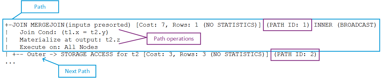
Both tables provide path-specific data. For example, QUERY_PLAN_PROFILES provides high-level data for each path, which includes:
-
Length of a query operation execution
-
How much memory that path's operation consumed
-
Size of data sent/received over the network
For example, you might observe that a GROUP BY HASH operation executed in 0.2 seconds using 100MB of memory.
Requirements
Real-time profiling minimally requires the ID of the transaction to monitor. If the transaction includes multiple statements, you also need the statement ID. You can get statement and transaction IDs by issuing
PROFILE on the query to profile. You can then use these identifiers to query system tables EXECUTION_ENGINE_PROFILES and QUERY_PLAN_PROFILES.
For more information, see Profiling single statements.
26.6.1 - Getting query plan status for small queries
Real-time profiling counters, stored in system table EXECUTION_ENGINE_PROFILES, are available for all currently executing statements, including internal operations, such as a .
Real-time profiling counters, stored in system table
EXECUTION_ENGINE_PROFILES, are available for all currently executing statements, including internal operations, such as a mergeout.
Profiling counters are available after query execution completes, if any one of the following conditions is true:
-
The query was run via the
PROFILE command
-
Systemwide profiling is enabled by Vertica meta-function
ENABLE_PROFILING.
-
The query ran more than two seconds.
Profiling counters are saved in system table EXECUTION_ENGINE_PROFILES until the storage quota is exceeded.
For example:
-
Profile the query to get transaction_id and statement_id from from EXECUTION_ENGINE_PROFILES. For example:
=> PROFILE SELECT * FROM t1 JOIN t2 ON t1.x = t2.y;
NOTICE 4788: Statement is being profiled
HINT: Select * from v_monitor.execution_engine_profiles where transaction_id=45035996273955065 and statement_id=4;
NOTICE 3557: Initiator memory for query: [on pool general: 248544 KB, minimum: 248544 KB]
NOTICE 5077: Total memory required by query: [248544 KB]
x | y | z
---+---+-------
3 | 3 | three
(1 row)
-
Query system table
QUERY_PLAN_PROFILES.
Note
For best results, sort on columns transaction_id, statement_id, path_id, and path_line_index.
=> SELECT ... FROM query_plan_profiles
WHERE transaction_id=45035996273955065 and statement_id=4;
ORDER BY transaction_id, statement_id, path_id, path_line_index;
26.6.2 - Getting query plan status for large queries
Real-time profiling is designed to monitor large (long-running) queries.
Real-time profiling is designed to monitor large (long-running) queries. Take the following steps to monitor plans for large queries:
-
Get the statement and transaction IDs for the query plan you want to profile by querying system table
CURRENT_SESSION:
=> SELECT transaction_id, statement_id from current_session;
transaction_id | statement_id
-------------------+--------------
45035996273955001 | 4
(1 row)
-
Run the query:
=> SELECT * FROM t1 JOIN t2 ON x=y JOIN ext on y=z;
-
Query system table
QUERY_PLAN_PROFILES, and sort on the transaction_id, statement_id, path_id, and path_line_index columns.
=> SELECT ... FROM query_plan_profiles WHERE transaction_id=45035996273955001 and statement_id=4
ORDER BY transaction_id, statement_id, path_id, path_line_index;
You can also use the Linux watch command to monitor long-running queries (see Real-time profiling).
Example
The following series of commands creates a table for a long-running query and then queries system table QUERY_PLAN_PROFILES:
-
Create table longq:
=> CREATE TABLE longq(x int);
CREATE TABLE
=> COPY longq FROM STDIN;
Enter data to be copied followed by a newline.
End with a backslash and a period on a line by itself.
>> 1
>> 2
>> 3
>> 4
>> 5
>> 6
>> 7
>> 8
>> 9
>> 10
>> \.
=> INSERT INTO longq SELECT f1.x+f2.x+f3.x+f4.x+f5.x+f6.x+f7.x
FROM longq f1
CROSS JOIN longq f2
CROSS JOIN longq f3
CROSS JOIN longq f4
CROSS JOIN longq f5
CROSS JOIN longq f6
CROSS JOIN longq f7;
OUTPUT
----------
10000000
(1 row)
=> COMMIT;
COMMIT
-
Suppress query output on the terminal window by using the vsql \o command:
=> \o /home/dbadmin/longQprof
-
Query the new table:
=> SELECT * FROM longq;
-
Get the transaction and statement IDs:
=> SELECT transaction_id, statement_id from current_session;
transaction_id | statement_id
-------------------+--------------
45035996273955021 | 4
(1 row)
-
Turn off the \o command so Vertica continues to save query plan information to the file you specified. Alternatively, leave it on and examine the file after you query system table QUERY_PLAN_PROFILES.
=> \o
-
Query system table QUERY_PLAN_PROFILES:
=> SELECT
transaction_id,
statement_id,
path_id,
path_line_index,
is_executing,
running_time,
path_line
FROM query_plan_profiles
WHERE transaction_id=45035996273955021 AND statement_id=4
ORDER BY transaction_id, statement_id, path_id, path_line_index;
26.6.3 - Improving readability of QUERY_PLAN_PROFILES output
Output from the QUERY_PLAN_PROFILES table can be very wide because of the path_line column.
Output from the
QUERY_PLAN_PROFILES table can be very wide because of the path_line column. To facilitate readability, query QUERY_PLAN_PROFILES using one or more of the following options:
-
Sort output by transaction_id, statement_id, path_id, and path_line_index:
=> SELECT ... FROM query_plan_profiles
WHERE ...
ORDER BY transaction_id, statement_id, path_id, path_line_index;
-
Use column aliases to decrease column width:
=> SELECT statement_id AS sid, path_id AS id, path_line_index AS order,
is_started AS start, is_completed AS end, is_executing AS exe,
running_time AS run, memory_allocated_bytes AS mem,
read_from_disk_bytes AS read, received_bytes AS rec,
sent_bytes AS sent, FROM query_plan_profiles
WHERE transaction_id=45035996273910558 AND statement_id=3
ORDER BY transaction_id, statement_id, path_id, path_line_index;
-
Use the vsql \o command to redirect
EXPLAIN output to a file:
=> \o /home/dbadmin/long-queries
=> EXPLAIN SELECT * FROM customer_dimension;
=> \o
26.6.4 - Managing query profile data
Vertica retains data for queries until the storage quota for the table is exceeded, when it automatically purges the oldest queries to make room for new ones.
Vertica retains data for queries until the storage quota for the table is exceeded, when it automatically purges the oldest queries to make room for new ones. You can also clear profiled data by calling one of the following functions:
-
CLEAR_PROFILING clears profiled data from memory. For example, the following command clears profiling for general query-run information, such as the query strings used and the duration of queries.
=> SELECT CLEAR_PROFILING('query');
-
CLEAR_DATA_COLLECTOR clears all memory and disk records on the Data Collector tables and functions and resets collection statistics in system table DATA_COLLECTOR.
-
FLUSH_DATA_COLLECTOR waits until memory logs are moved to disk and then flushes the Data Collector, synchronizing the DataCollector log with the disk storage.
Configuring data retention policies
Vertica retains the historical data it gathers as specified by the configured retention policies.
26.6.5 - Analyzing suboptimal query plans
If profiling uncovers a suboptimal query, invoking one of the following functions might help:.
If profiling uncovers a suboptimal query, invoking one of the following functions might help:
-
ANALYZE_WORKLOAD analyzes system information held in system tables and provides tuning recommendations that are based on a combination of statistics, system and data collector events, and database-table-projection design.
-
ANALYZE_STATISTICS collects and aggregates data samples and storage information from all nodes that store projections associated with the specified table or column.
You can also run your query through the Database Designer. See Incremental Design.
26.7 - Sample views for counter information
The EXECUTION_ENGINE_PROFILES table contains the data for each profiling counter as a row within the table.
The EXECUTION_ENGINE_PROFILES table contains the data for each profiling counter as a row within the table. For example, the execution time (us) counter is in one row, and the rows produced counter is in a second row. Since there are many different profiling counters, many rows of profiling data exist for each operator. Some sample views are installed by default to simplify the viewing of profiling counters.
Running scripts to create the sample views
The following script creates the v_demo schema and places the views in that schema.
/opt/vertica/scripts/demo_eeprof_view.sql
Viewing counter values using the sample views
There is one view for each of the profiling counters to simplify viewing of a single counter value. For example, to view the execution time for all operators, issue the following command from the database:
=> SELECT * FROM v_demo.eeprof_execution_time_us;
To view all counter values available for all profiled queries:
=> SELECT * FROM v_demo.eeprof_counters;
To select all distinct operators available for all profiled queries:
=> SELECT * FROM v_demo.eeprof_operators;
Combining sample views
These views can be combined:
=> SELECT * FROM v_demo.eeprof_execution_time_us
NATURAL LEFT OUTER JOIN v_demo.eeprof_rows_produced;
To view the execution time and rows produced for a specific transaction and statement_id ranked by execution time on each node:
=> SELECT * FROM v_demo.eeprof_execution_time_us_rank
WHERE transaction_id=45035996273709699
AND statement_id=1
ORDER BY transaction_id, statement_id, node_name, rk;
To view the top five operators by execution time on each node:
=> SELECT * FROM v_demo.eeprof_execution_time_us_rank
WHERE transaction_id=45035996273709699
AND statement_id=1 AND rk<=5
ORDER BY transaction_id, statement_id, node_name, rk;
27 - About locale
Vertica locale specifications follow a subset of the Unicode LDML standard as implemented by the ICU library.
Locale specifies the user's language, country, and any special variant preferences, such as collation. Vertica uses locale to determine the behavior of certain string functions. Locale also determines the collation for various SQL commands that require ordering and comparison, such as aggregate GROUP BY and ORDER BY clauses, joins, and the analytic ORDER BY clause.
The default locale for a Vertica database is en_US@collation=binary (English US). You can define a new default locale that is used for all sessions on the database. You can also override the locale for individual sessions. However, projections are always collated using the default en_US@collation=binary collation, regardless of the session collation. Any locale-specific collation is applied at query time.
If you set the locale to null, Vertica sets the locale to en_US_POSIX. You can set the locale back to the default locale and collation by issuing the vsql meta-command \locale. For example:
Note
=> set locale to '';
INFO 2567: Canonical locale: 'en_US_POSIX'
Standard collation: 'LEN'
English (United States, Computer)
SET
=> \locale en_US@collation=binary;
INFO 2567: Canonical locale: 'en_US'
Standard collation: 'LEN_KBINARY'
English (United States)
=> \locale
en_US@collation-binary;
You can set locale through ODBC, JDBC, and ADO.net.
Vertica locale specifications follow a subset of the Unicode LDML standard as implemented by the ICU library.
27.1 - Locale handling in Vertica
The following sections describes how Vertica handles locale.
The following sections describes how Vertica handles locale.
Session locale
Locale is session-scoped and applies only to queries executed in that session. You cannot specify locale for individual queries. When you start a session it obtains its locale from the configuration parameter DefaultSessionLocale.
Query restrictions
The following restrictions apply when queries are run with locale other than the default en_US@collation=binary:
-
When one or more of the left-side NOT IN columns is CHAR or VARCHAR, multi-column NOT IN subqueries are not supported . For example:
=> CREATE TABLE test (x VARCHAR(10), y INT);
=> SELECT ... FROM test WHERE (x,y) NOT IN (SELECT ...);
ERROR: Multi-expression NOT IN subquery is not supported because a left
hand expression could be NULL
Note
Even if columns test.x and test.y have a NOT NULL constraint, an error occurs.
-
If the outer query contains a GROUP BY clause on a CHAR or VARCHAR column, correlated HAVING clause subqueries are not supported. In the following example, the GROUP BY x in the outer query causes the error:
=> DROP TABLE test CASCADE;
=> CREATE TABLE test (x VARCHAR(10));
=> SELECT COUNT(*) FROM test t GROUP BY x HAVING x
IN (SELECT x FROM test WHERE t.x||'a' = test.x||'a' );
ERROR: subquery uses ungrouped column "t.x" from outer query
-
Subqueries that use analytic functions in the HAVING clause are not supported. For example:
=> DROP TABLE test CASCADE;
=> CREATE TABLE test (x VARCHAR(10));
=> SELECT MAX(x)OVER(PARTITION BY 1 ORDER BY 1) FROM test
GROUP BY x HAVING x IN (SELECT MAX(x) FROM test);
ERROR: Analytics query with having clause expression that involves
aggregates and subquery is not supported
Collation and projections
Projection data is sorted according to the default en_US@collation=binary collation. Thus, regardless of the session setting, issuing the following command creates a projection sorted by col1 according to the binary collation:
=> CREATE PROJECTION p1 AS SELECT * FROM table1 ORDER BY col1;
In such cases, straße and strasse are not stored near each other on disk.
Sorting by binary collation also means that sort optimizations do not work in locales other than binary. Vertica returns the following warning if you create tables or projections in a non-binary locale:
WARNING: Projections are always created and persisted in the default
Vertica locale. The current locale is de_DE
When the locale is non-binary, Vertica uses the
COLLATION function to transform input to a binary string that sorts in the proper order.
This transformation increases the number of bytes required for the input according to this formula:
result_column_width = input_octet_width * CollationExpansion + 4
The default value of configuration parameter CollationExpansion is 5.
Character data type handling
-
CHAR fields are displayed as fixed length, including any trailing spaces. When CHAR fields are processed internally, they are first stripped of trailing spaces. For VARCHAR fields, trailing spaces are usually treated as significant characters; however, trailing spaces are ignored when sorting or comparing either type of character string field using a non-binary locale.
-
The maximum length parameter for VARCHAR and CHAR data type refers to the number of octets (bytes) that can be stored in that field and not number of characters. When using multi-byte UTF-8 characters, the fields must be sized to accommodate from 1 to 4 bytes per character, depending on the data.
27.2 - Specifying locale: long form
Vertica supports long forms that specify the collation keyword.
Vertica supports long forms that specify the collation keyword. Vertica extends long-form processing to accept collation arguments.
Syntax
[language][_script][_country][_variant][@collation‑spec]
Note
The following syntax options apply:
-
Locale specification strings are case insensitive. For example, en_us and EN_US, are equivalent.
-
You can substitute underscores with hyphens. For example: [-script]
Parameters
language- A two- or three-letter lowercase code for a particular language. For example, Spanish is
es English is en and French is fr. The two-letter language code uses the ISO-639 standard.
_script- An optional four-letter script code that follows the language code. If specified, it should be a valid script code as listed on the Unicode ISO 15924 Registry.
_country- A specific language convention within a generic language for a specific country or region. For example, French is spoken in many countries, but the currencies are different in each country. To allow for these differences among specific geographical, political, or cultural regions, locales are specified by two-letter, uppercase codes. For example,
FR represents France and CA represents Canada. The two letter country code uses the ISO-3166 standard.
_variant- Differences may also appear in language conventions used within the same country. For example, the Euro currency is used in several European countries while the individual country's currency is still in circulation. To handle variations inside a language and country pair, add a third code, the variant code. The variant code is arbitrary and completely application-specific. ICU adds
_EURO to its locale designations for locales that support the Euro currency. Variants can have any number of underscored key words. For example, EURO_WIN is a variant for the Euro currency on a Windows computer.
Another use of the variant code is to designate the Collation (sorting order) of a locale. For instance, the es__TRADITIONAL locale uses the traditional sorting order which is different from the default modern sorting of Spanish.
@collation‑spec- Vertica only supports the keyword
collation, as follows:
@collation=collation‑type[;arg]...
Collation can specify one or more semicolon-delimited arguments, described below.
collation‑type is set to one of the following values:
-
big5han: Pinyin ordering for Latin, big5 charset ordering for CJK characters (used in Chinese).
-
dict: For a dictionary-style ordering (such as in Sinhala).
-
direct: Hindi variant.
-
gb2312/gb2312han: Pinyin ordering for Latin, gb2312han charset ordering for CJK characters (used in Chinese).
-
phonebook: For a phonebook-style ordering (such as in German).
-
pinyin: Pinyin ordering for Latin and for CJK characters; that is, an ordering for CJK characters based on a character-by-character transliteration into a pinyin (used in Chinese).
-
reformed: Reformed collation (such as in Swedish).
-
standard: The default ordering for each language. For root it is [UCA] order; for each other locale it is the same as UCA (Unicode Collation Algorithm) ordering except for appropriate modifications to certain characters for that language. The following are additional choices for certain locales; they have effect only in certain locales.
-
stroke: Pinyin ordering for Latin, stroke order for CJK characters (used in Chinese) not supported.
-
traditional: For a traditional-style ordering (such as in Spanish).
-
unihan: Pinyin ordering for Latin, Unihan radical-stroke ordering for CJK characters (used in Chinese) not supported.
-
binary: Vertica default, providing UTF-8 octet ordering.
Notes:
-
Collations might default to root, the ICU default collation.
-
Invalid values of the collation keyword and its synonyms do not cause an error. For example, the following does not generate an error. It simply ignores the invalid value:
=> \locale en_GB@collation=xyz
INFO 2567: Canonical locale: 'en_GB@collation=xyz'
Standard collation: 'LEN'
English (United Kingdom, collation=xyz)
For more about collation options, see Unicode Locale Data Markup Language (LDML).
Collation arguments
collation can specify one or more of the following arguments :
|
Parameter |
Short form |
Description |
colstrength |
S |
Sets the default strength for comparison. This feature is locale dependent.
Set colstrength to one of the following:
-
1 | primary: Ignores case and accents. Only primary differences are used during comparison—for example, a versus z.
-
2 | secondary: Ignores case. Only secondary and above differences are considered for comparison—for example, different accented forms of the same base letter such as a versus \u00E4.
-
3 | tertiary (default): Only tertiary differences and higher are considered for comparison. Tertiary comparisons are typically used to evaluate case differences—for example, Z versus z.
-
4 | quarternary: For example, used with Hiragana.
|
colAlternate |
A |
Sets alternate handling for variable weights, as described in UCA, one of the following:
-
non-ignorable | N | D
-
shifted | S
|
colBackwards |
F |
For Latin with accents, this parameter determines which accents are sorted. It sets the comparison for the second level to be backwards.
Note
colBackwards is automatically set for French accents.
Set
colBackwards
-
on | O: The normal UCA algorithm is used.
-
off | X: All strings that are in Fast C or D normalization form (FCD) sort correctly, but others do not necessarily sort correctly. Set to off if the strings to be compared are in FCD.
|
colNormalization |
N |
Set to one of the following:
-
on | O: The normal UCA algorithm is used.
-
off | X: All strings that are in Fast C or D normalization form (FCD) sort correctly, but others won't necessarily sort correctly. It should only be set off if the strings to be compared are in FCD.
|
colCaseLevel |
E |
Set to one of the following:
-
on | O: A level consisting only of case characteristics is inserted in front of tertiary level. To ignore accents but take cases into account, set strength to primary and case level to on.
-
off | X: This level is omitted.
|
colCaseFirst |
C |
Set to one of the following:
-
upper | U: Upper case sorts before lower case.
-
lower | L: Lower case sorts before upper case. This is useful for locales that have already supported ordering but require different order of cases. It affects case and tertiary levels.
-
off | short: Tertiary weights unaffected
|
colHiraganaQuarternary |
H |
Controls special treatment of Hiragana code points on quaternary level, one of the following:
-
on | O: Hiragana codepoints get lower values than all the other non-variable code points. The strength must be greater or equal than quaternary for this attribute to take effect.
-
off | X: Hiragana letters are treated normally.
|
colNumeric |
D |
If set to on, any sequence of Decimal Digits (General_Category = Nd in the [UCD]) is sorted at a primary level with its numeric value. For example, A‑21 < A‑123. |
variableTop |
B |
Sets the default value for the variable top. All code points with primary weights less than or equal to the variable top will be considered variable, and are affected by the alternate handling.
For example, the following command sets variableTop to be HYPHEN (u2010)
=> \locale en_US@colalternate=shifted;variabletop=u2010
|
Locale processing notes
-
Incorrect locale strings are accepted if the prefix can be resolved to a known locale version.
For example, the following works because the language can be resolved:
=> \locale en_XX
INFO 2567: Canonical locale: 'en_XX'
Standard collation: 'LEN'
English (XX)
The following does not work because the language cannot be resolved:
=> \locale xx_XX
xx_XX: invalid locale identifier
-
POSIX-type locales such as en_US.UTF-8 work to some extent in that the encoding part "UTF-8" is ignored.
-
Vertica uses the icu4c-4_2_1 library to support basic locale/collation processing with some extensions. This does not currently meet current standards for locale processing (https://tools.ietf.org/html/rfc5646).
Examples
Specify German locale as used in Germany (de), with phonebook-style collation:
=> \locale de_DE@collation=phonebook
INFO 2567: Canonical locale: 'de_DE@collation=phonebook'
Standard collation: 'KPHONEBOOK_LDE'
German (Germany, collation=Phonebook Sort Order)
Deutsch (Deutschland, Sortierung=Telefonbuch-Sortierregeln)
Specify German locale as used in Germany (de), with phonebook-style collation and strength set to secondary:
=> \locale de_DE@collation=phonebook;colStrength=secondary
INFO 2567: Canonical locale: 'de_DE@collation=phonebook'
Standard collation: 'KPHONEBOOK_LDE_S2'
German (Germany, collation=Phonebook Sort Order)
Deutsch (Deutschland, Sortierung=Telefonbuch-Sortierregeln)
27.3 - Specifying locale: short form
Vertica accepts locales in short form.
Vertica accepts locales in short form. You can use the short form to specify the locale and keyname pair/value names.
To determine the short form for a locale, type in the long form and view the last line of INFO, as follows:
\locale frINFO: Locale: 'fr'
INFO: French
INFO: français
INFO: Short form: 'LFR'
Examples
Specify en (English) locale:
\locale LENINFO: Locale: 'en'
INFO: English
INFO: Short form: 'LEN'
Specify German locale as used in Germany (de), with phonebook-style collation:
\locale LDE_KPHONEBOOKINFO: Locale: 'de@collation=phonebook'
INFO: German (collation=Phonebook Sort Order)
INFO: Deutsch (Sortierung=Telefonbuch-Sortierregeln)
INFO: Short form: 'KPHONEBOOK_LDE'
Specify German locale as used in Germany (de), with phonebook-style collation:
\locale LDE_KPHONEBOOK_S2INFO: Locale: 'de@collation=phonebook'
INFO: German (collation=Phonebook Sort Order)
INFO: Deutsch (Sortierung=Telefonbuch-Sortierregeln)
INFO: Short form: 'KPHONEBOOK_LDE_S2'
27.4 - Supported locales
The following are the supported locale strings for Vertica.
The following are the supported locale strings for Vertica. Each locale can optionally have a list of key/value pairs (see Specifying locale: long form).
|
Locale Name |
Language or Variant |
Region |
|
af |
Afrikaans |
|
|
af_NA |
Afrikaans |
Namibian Afrikaans |
|
af_ZA |
Afrikaans |
South Africa |
|
am |
Ethiopic |
|
|
am_ET |
Ethiopic |
Ethiopia |
|
ar |
Arabic |
|
|
ar_AE |
Arabic |
United Arab Emirates |
|
ar_BH |
Arabic |
Bahrain |
|
ar_DZ |
Arabic |
Algeria |
|
ar_EG |
Arabic |
Egypt |
|
ar_IQ |
Arabic |
Iraq |
|
ar_JO |
Arabic |
Jordan |
|
ar_KW |
Arabic |
Kuwait |
|
ar_LB |
Arabic |
Lebanon |
|
ar_LY |
Arabic |
Libya |
|
ar_MA |
Arabic |
Morocco |
|
ar_OM |
Arabic |
Oman |
|
ar_QA |
Arabic |
Qatar |
|
ar_SA |
Arabic |
Saudi Arabia |
|
ar_SD |
Arabic |
Sudan |
|
ar_SY |
Arabic |
Syria |
|
ar_TN |
Arabic |
Tunisia |
|
ar_YE |
Arabic |
Yemen |
|
as |
Assamese |
|
|
as_IN |
Assamese |
India |
|
az |
Azerbaijani |
|
|
az_Cyrl |
Azerbaijani |
Cyrillic |
|
az_Cyrl_AZ |
Azerbaijani |
Azerbaijan Cyrillic |
|
az_Latn |
Azerbaijani |
Latin |
|
az_Latn_AZ |
Azerbaijani |
Azerbaijan Latin |
|
be |
Belarusian |
|
|
be_BY |
Belarusian |
Belarus |
|
bg |
Bulgarian |
|
|
bg_BG |
Bulgarian |
Bulgaria |
|
bn |
Bengali |
|
|
bn_BD |
Bengali |
Bangladesh |
|
bn_IN |
Bengali |
India |
|
bo |
Tibetan |
|
|
bo_CN |
Tibetan |
PR China |
|
bo_IN |
Tibetan |
India |
|
ca |
Catalan |
|
|
ca_ES |
Catalan |
Spain |
|
cs |
Czech |
|
|
cs_CZ |
Czech |
Czech Republic |
|
cy |
Welsh |
|
|
cy_GB |
Welsh |
United Kingdom |
|
da |
Danish |
|
|
da_DK |
Danish |
Denmark |
|
de |
German |
|
|
de_AT |
German |
Austria |
|
de_BE |
German |
Belgium |
|
de_CH |
German |
Switzerland |
|
de_DE |
German |
Germany |
|
de_LI |
German |
Liechtenstein |
|
de_LU |
German |
Luxembourg |
|
el |
Greek |
|
|
el_CY |
Greek |
Cyprus |
|
el_GR |
Greek |
Greece |
|
en |
English |
|
|
en_AU |
English |
Australia |
|
en_BE |
English |
Belgium |
|
en_BW |
English |
Botswana |
|
en_BZ |
English |
Belize |
|
en_CA |
English |
Canada |
|
en_GB |
English |
United Kingdom |
|
en_HK |
English |
Hong Kong S.A.R. of China |
|
en_IE |
English |
Ireland |
|
en_IN |
English |
India |
|
en_JM |
English |
Jamaica |
|
en_MH |
English |
Marshall Islands |
|
en_MT |
English |
Malta |
|
en_NA |
English |
Namibia |
|
en_NZ |
English |
New Zealand |
|
en_PH |
English |
Philippines |
|
en_PK |
English |
Pakistan |
|
en_SG |
English |
Singapore |
|
en_TT |
English |
Trinidad and Tobago |
|
en_US |
English |
United States |
|
en_US_POSIX |
English |
United States Posix |
|
en_VI |
English |
U.S. Virgin Islands |
|
en_ZA |
English |
Zimbabwe or South Africa |
|
en_ZW |
English |
Zimbabwe |
|
eo |
Esperanto |
|
|
es |
Spanish |
|
|
es_AR |
Spanish |
Argentina |
|
es_BO |
Spanish |
Bolivia |
|
es_CL |
Spanish |
Chile |
|
es_CO |
Spanish |
Columbia |
|
es_CR |
Spanish |
Costa Rica |
|
es_DO |
Spanish |
Dominican Republic |
|
es_EC |
Spanish |
Ecuador |
|
es_ES |
Spanish |
Spain |
|
es_GT |
Spanish |
Guatemala |
|
es_HN |
Spanish |
Honduras |
|
es_MX |
Spanish |
Mexico |
|
es_NI |
Spanish |
Nicaragua |
|
es_PA |
Spanish |
Panama |
|
es_PE |
Spanish |
Peru |
|
es_PR |
Spanish |
Puerto Rico |
|
es_PY |
Spanish |
Paraguay |
|
es_SV |
Spanish |
El Salvador |
|
es_US |
Spanish |
United States |
|
es_UY |
Spanish |
Uruguay |
|
es_VE |
Spanish |
Venezuela |
|
et |
Estonian |
|
|
et_EE |
Estonian |
Estonia |
|
eu |
Basque |
Spain |
|
eu_ES |
Basque |
Spain |
|
fa |
Persian |
|
|
fa_AF |
Persian |
Afghanistan |
|
fa_IR |
Persian |
Iran |
|
fi |
Finnish |
|
|
fi_FI |
Finnish |
Finland |
|
fo |
Faroese |
|
|
fo_FO |
Faroese |
Faroe Islands |
|
fr |
French |
|
|
fr_BE |
French |
Belgium |
|
fr_CA |
French |
Canada |
|
fr_CH |
French |
Switzerland |
|
fr_FR |
French |
France |
|
fr_LU |
French |
Luxembourg |
|
fr_MC |
French |
Monaco |
|
fr_SN |
French |
Senegal |
|
ga |
Gaelic |
|
|
ga_IE |
Gaelic |
Ireland |
|
gl |
Gallegan |
|
|
gl_ES |
Gallegan |
Spain |
|
gsw |
German |
|
|
gsw_CH |
German |
Switzerland |
|
gu |
Gujurati |
|
|
gu_IN |
Gujurati |
India |
|
gv |
Manx |
|
|
gv_GB |
Manx |
United Kingdom |
|
ha |
Hausa |
|
|
ha_Latn |
Hausa |
Latin |
|
ha_Latn_GH |
Hausa |
Ghana (Latin) |
|
ha_Latn_NE |
Hausa |
Niger (Latin) |
|
ha_Latn_NG |
Hausa |
Nigeria (Latin)
|
|
haw |
Hawaiian |
Hawaiian |
|
haw_US |
Hawaiian |
United States |
|
he |
Hebrew |
|
|
he_IL |
Hebrew |
Israel |
|
hi |
Hindi |
|
|
hi_IN |
Hindi |
India |
|
hr |
Croation |
|
|
hr_HR |
Croation |
Croatia |
|
hu |
Hungarian |
|
|
hu_HU |
Hungarian |
Hungary |
|
hy |
Armenian |
|
|
hy_AM |
Armenian |
Armenia |
|
hy_AM_REVISED |
Armenian |
Revised Armenia |
|
id |
Indonesian |
|
|
id_ID |
Indonesian |
Indonesia |
|
ii |
Sichuan |
|
|
ii_CN |
Sichuan |
Yi |
|
is |
Icelandic |
|
|
is_IS |
Icelandic |
Iceland |
|
it |
Italian |
|
|
it_CH |
Italian |
Switzerland |
|
it_IT |
Italian |
Italy |
|
ja |
Japanese |
|
|
ja_JP |
Japanese |
Japan |
|
ka |
Georgian |
|
|
ka_GE |
Georgian |
Georgia |
|
kk |
Kazakh |
|
|
kk_Cyrl |
Kazakh |
Cyrillic |
|
kk_Cyrl_KZ |
Kazakh |
Kazakhstan (Cyrillic) |
|
kl |
Kalaallisut |
|
|
kl_GL |
Kalaallisut |
Greenland |
|
km |
Khmer |
|
|
km_KH |
Khmer |
Cambodia |
|
kn |
Kannada |
|
|
kn-IN |
Kannada |
India |
|
ko |
Korean |
|
|
ko_KR |
Korean |
Korea |
|
kok |
Konkani |
|
|
kok_IN |
Konkani |
India |
|
kw |
Cornish |
|
|
kw_GB |
Cornish |
United Kingdom |
|
lt |
Lithuanian |
|
|
lt_LT |
Lithuanian |
Lithuania |
|
lv |
Latvian |
|
|
lv_LV |
Latvian |
Latvia |
|
mk |
Macedonian |
|
|
mk_MK |
Macedonian |
Macedonia |
|
ml |
Malayalam |
|
|
ml_IN |
Malayalam |
India |
|
mr |
Marathi |
|
|
mr_IN |
Marathi |
India |
|
ms |
Malay |
|
|
ms_BN |
Malay |
Brunei |
|
ms_MY |
Malay |
Malaysia |
|
mt |
Maltese |
|
|
mt_MT |
Maltese |
Malta |
|
nb |
Norwegian Bokml |
|
|
nb_NO |
Norwegian Bokml |
Norway |
|
ne |
Nepali |
|
|
ne_IN |
Nepali |
India |
|
ne_NP |
Nepali |
Nepal |
|
nl |
Dutch |
|
|
nl_BE |
Dutch |
Belgium |
|
nl_NL |
Dutch |
Netherlands |
|
nn |
Norwegian nynorsk |
|
|
nn_NO |
Norwegian nynorsk |
Norway |
|
om |
Oromo |
|
|
om_ET |
Oromo |
Ethiopia |
|
om_KE |
Oromo |
Kenya |
|
or |
Oriya |
|
|
or_IN |
Oriya |
India |
|
pa |
Punjabi |
|
|
pa_Arab |
Punjabi |
Arabic |
|
pa_Arab_PK |
Punjabi |
Pakistan (Arabic) |
|
pa_Guru |
Punjabi |
Gurmukhi |
|
pa_Guru_IN |
Punjabi |
India (Gurmukhi) |
|
pl |
Polish |
|
|
pl_PL |
Polish |
Poland |
|
ps |
Pashto |
|
|
ps_AF |
Pashto |
Afghanistan |
|
pt |
Portuguese |
|
|
pt_BR |
Portuguese |
Brazil |
|
pt_PT |
Portuguese |
Portugal |
|
ro |
Romanian |
|
|
ro_MD |
Romanian |
Moldavia |
|
ro_RO |
Romanian |
Romania |
|
ru |
Russian |
|
|
ru_RU |
Russian |
Russia |
|
ru_UA |
Russian |
Ukraine |
|
si |
Sinhala |
|
|
si_LK |
Sinhala |
Sri Lanka |
|
sk |
Slovak |
|
|
sk_SK |
Slovak |
Slovakia |
|
sl |
Slovenian |
|
|
sl_SL |
Slovenian |
Slovenia |
|
so |
Somali |
|
|
so_DJ |
Somali |
Djibouti |
|
so_ET |
Somali |
Ethiopia |
|
so_KE |
Somali |
Kenya |
|
so_SO |
Somali |
Somalia |
|
sq |
Albanian |
|
|
sq_AL |
Albanian |
Albania |
|
sr |
Serbian |
|
|
sr_Cyrl |
Serbian |
Cyrillic |
|
sr_Cyrl_BA |
Serbian |
Bosnia and Herzegovina (Cyrillic) |
|
sr_Cyrl_ME |
Serbian |
Montenegro (Cyrillic) |
|
sr_Cyrl_RS |
Serbian |
Serbia (Cyrillic)
|
|
sr_Latn |
Serbian |
Latin |
|
sr_Latn_BA |
Serbian |
Bosnia and Herzegovina (Latin) |
|
sr_Latn_ME |
Serbian |
Montenegro (Latin) |
|
sr_Latn_RS |
Serbian |
Serbia (Latin)
|
|
sv |
Swedish |
|
|
sv_FI |
Swedish |
Finland |
|
sv_SE |
Swedish |
Sweden |
|
sw |
Swahili |
|
|
sw_KE |
Swahili |
Kenya |
|
sw_TZ |
Swahili |
Tanzania |
|
ta |
Tamil |
|
|
ta_IN |
Tamil |
India |
|
te |
Telugu |
|
|
te_IN |
Telugu |
India |
|
th |
Thai |
|
|
th_TH |
Thai |
Thailand |
|
ti |
Tigrinya |
|
|
ti_ER |
Tigrinya |
Eritrea |
|
ti_ET |
Tigrinya |
Ethiopia |
|
tr |
Turkish |
|
|
tr_TR |
Turkish |
Turkey |
|
uk |
Ukrainian |
|
|
uk_UA |
Ukrainian |
Ukraine |
|
ur |
Urdu |
|
|
ur_IN |
Urdu |
India |
|
ur_PK |
Urdu |
Pakistan |
|
uz |
Uzbek |
|
|
uz_Arab |
Uzbek |
Arabic |
|
uz_Arab_AF |
Uzbek |
Afghanistan (Arabic) |
|
uz_Cryl |
Uzbek |
Cyrillic |
|
uz_Cryl_UZ |
Uzbek |
Uzbekistan (Cyrillic) |
|
uz_Latin |
Uzbek |
Latin |
|
us_Latin_UZ |
|
Uzbekistan (Latin) |
|
vi |
Vietnamese |
|
|
vi_VN |
Vietnamese |
Vietnam |
|
zh |
Chinese |
|
|
zh_Hans |
Chinese |
Simplified Han |
|
zh_Hans_CN |
Chinese |
China (Simplified Han) |
|
zh_Hans_HK |
Chinese |
Hong Kong SAR China (Simplified Han) |
|
zh_Hans_MO |
Chinese |
Macao SAR China (Simplified Han) |
|
zh_Hans_SG |
Chinese |
Singapore (Simplified Han) |
|
zh_Hant |
Chinese |
Traditional Han |
|
zh_Hant_HK |
Chinese |
Hong Kong SAR China (Traditional Han) |
|
zh_Hant_MO |
Chinese |
Macao SAR China (Traditional Han) |
|
zh_Hant_TW |
Chinese |
Taiwan (Traditional Han) |
|
zu |
Zulu |
|
|
zu_ZA |
Zulu |
South Africa |
27.5 - Locale and UTF-8 support
Vertica supports Unicode Transformation Format-8, or UTF8, where 8 equals 8-bit.
Vertica supports Unicode Transformation Format-8, or UTF8, where 8 equals 8-bit. UTF-8 is a variable-length character encoding for Unicode created by Ken Thompson and Rob Pike. UTF-8 can represent any universal character in the Unicode standard. Initial encoding of byte codes and character assignments for UTF-8 coincides with ASCII. Thus, UTF8 requires little or no change for software that handles ASCII but preserves other values.
Vertica database servers expect to receive all data in UTF-8, and Vertica outputs all data in UTF-8. The ODBC API operates on data in UCS-2 on Windows systems, and normally UTF-8 on Linux systems. JDBC and ADO.NET APIs operate on data in UTF-16. Client drivers automatically convert data to and from UTF-8 when sending to and receiving data from Vertica using API calls. The drivers do not transform data loaded by executing a COPY or COPY LOCAL statement.
UTF-8 string functions
The following string functions treat VARCHAR arguments as UTF-8 strings (when USING OCTETS is not specified) regardless of locale setting.
|
String function |
Description |
LOWER |
Returns a VARCHAR value containing the argument converted to lowercase letters. |
UPPER |
Returns a VARCHAR value containing the argument converted to uppercase letters. |
INITCAP |
Capitalizes first letter of each alphanumeric word and puts the rest in lowercase. |
INSTR |
Searches string for substring and returns an integer indicating the position of the character in string that is the first character of this occurrence. |
SPLIT_PART |
Splits string on the delimiter and returns the location of the beginning of the given field (counting from one). |
POSITION |
Returns an integer value representing the character location of a specified substring with a string (counting from one). |
STRPOS |
Returns an integer value representing the character location of a specified substring within a string (counting from one). |
27.6 - Locale-aware string functions
Vertica provides string functions to support internationalization.
Vertica provides string functions to support internationalization. Unless otherwise specified, these string functions can optionally specify whether VARCHAR arguments should be interpreted as octet (byte) sequences, or as (locale-aware) sequences of characters. Specify this information by adding the parameter USING OCTETS and USING CHARACTERS (default) to the function.
The following table lists all string functions that are locale-aware:
|
String function |
Description |
BTRIM |
Removes the longest string consisting only of specified characters from the start and end of a string. |
CHARACTER_LENGTH |
Returns an integer value representing the number of characters or octets in a string. |
GREATEST |
Returns the largest value in a list of expressions. |
GREATESTB |
Returns its greatest argument, using binary ordering, not UTF-8 character ordering. |
INITCAP |
Capitalizes first letter of each alphanumeric word and puts the rest in lowercase. |
INSTR |
Searches string for substring and returns an integer indicating the position of the character in string that is the first character of this occurrence. |
LEAST |
Returns the smallest value in a list of expressions. |
LEASTB |
Returns its least argument, using binary ordering, not UTF-8 character ordering. |
LEFT |
Returns the specified characters from the left side of a string. |
LENGTH |
Takes one argument as an input and returns returns an integer value representing the number of characters in a string. |
LTRIM |
Returns a VARCHAR value representing a string with leading blanks removed from the left side (beginning). |
OVERLAY |
Returns a VARCHAR value representing a string having had a substring replaced by another string. |
OVERLAYB |
Returns an octet value representing a string having had a substring replaced by another string. |
REPLACE |
replaces all occurrences of characters in a string with another set of characters. |
RIGHT |
Returns the length right-most characters of string. |
SUBSTR |
Returns a VARCHAR value representing a substring of a specified string. |
SUBSTRB |
Returns a byte value representing a substring of a specified string. |
SUBSTRING |
Given a value, a position, and an optional length, returns a value representing a substring of the specified string at the given position. |
TRANSLATE |
Replaces individual characters in string_to_replace with other characters. |
UPPER |
Returns a VARCHAR value containing the argument converted to uppercase letters. |
28 - Appendix: creating native binary format files
Using COPY to load data with the NATIVE parser requires that the input data files conform to the requirements described in this appendix.
Using
COPY to load data with the NATIVE parser requires that the input data files conform to the requirements described in this appendix. All NATIVE files must contain:
The subsection Loading a NATIVE file into a table: example describes an example of loading data with the NATIVE parser.
Note
You cannot mix Binary and ASCII source files in the same COPY statement.
28.1 - File signature
The first part of a NATIVE binary file consists of a file signature.
The first part of a NATIVE binary file consists of a file signature. The contents of the signature are fixed, and listed in the following table.
|
Byte Offset |
0 |
1 |
2 |
3 |
4 |
5 |
6 |
7 |
8 |
9 |
10 |
|
Hex Value |
4E |
41 |
54 |
49 |
56 |
45 |
0A |
FF |
0D |
0A |
00 |
|
Text Literals |
N |
A |
T |
I |
V |
E |
E'\n' |
E'\317' |
E'\r' |
E'\n' |
E'\000' |
The signature ensures that the file has neither been corrupted by a non-8-bit file transfer, nor stripped of carriage returns, linefeeds, or null values. If the signature is intact, Vertica determines that the file has not been corrupted.
28.2 - Column definitions
Following the file signature, the file must define the widths of each column in the file as follows.
Following the file signature, the file must define the widths of each column in the file as follows.
|
Byte Offset |
Length (bytes) |
Description |
Comments |
|
11 |
4 |
Header area length |
32-bit integer in little-endian format that contains the length in bytes of remaining in the header, not including itself. This is the number of bytes from the end of this value to the start of the row data. |
|
15 |
2 |
NATIVE file version |
16-bit integer in little-endian format containing the version number of the NATIVE file format. The only valid value is currently 1. Future changes to the format could be assigned different version numbers to maintain backward compatibility. |
|
17 |
1 |
Filler |
Always 0. |
|
18 |
2 |
Number of columns |
16-bit integer in little-endian format that contains the number of columns in each row in the file. |
|
20+ |
4 bytes for each column of data in the table |
Column widths |
Array of 32-bit integers in little-endian format that define the width of each column in the row. Variable-width columns have a value of -1 (0xFF 0xFF 0xFF 0xFF). |
Note
All integers in NATIVE files are in little-endian format (least significant byte first).
The width of each column is determined by the data type it contains. The following table explains the column width needed for each data type, along with the data encoding.
|
Data Type |
Length (bytes) |
Column Content |
|
INTEGER |
1, 2, 4, 8 |
8-, 16-, 32-, and 64-bit integers are supported. All multi-byte values are stored in little-endian format.
Note: All values for a column must be the width you specify here. If you set the length of an INTEGER column to be 4 bytes, then all of the values you supply for that column must be 32-bit integers.
|
|
BOOLEAN |
1 |
0 for false, 1 for true. |
|
FLOAT |
8 |
Encoded in IEEE-754 format. |
|
CHAR |
User-specified |
-
Strings shorter than the specified length must be right-padded with spaces (E'\040').
-
Strings are not null-terminated.
-
Character encoding is UTF-8.
-
UTF-8 strings can contain multi-byte characters. Therefore, number of characters in the string may not equal the number of bytes.
|
|
VARCHAR |
4-byte integer (length) + data |
The column width for a VARCHAR column is always -1 to signal that it contains variable-length data.
-
Each VARCHAR column value starts with a 32-bit integer that contains the number of bytes in the string.
-
The string must not be null-terminated.
-
Character encoding must be UTF-8.
-
Remember that UTF-8 strings can contain multi-byte characters. Therefore, number of characters in the string may not equal the number of bytes.
|
|
DATE |
8 |
64-bit integer in little-endian format containing the Julian day since Jan 01 2000 (J2451545) |
|
TIME |
8 |
64-bit integer in little-endian format containing the number of microseconds since midnight in the UTC time zone. |
|
TIMETZ |
8 |
64-bit value where
-
Upper 40 bits contain the number of microseconds since midnight.
-
Lower 24 bits contain time zone as the UTC offset in microseconds calculated as follows: Time zone is logically from -24hrs to +24hrs from UTC. Instead it is represented here as a number between 0hrs to 48hrs. Therefore, 24hrs should be added to the actual time zone to calculate it.
Each portion is stored in little-endian format (5 bytes followed by 3 bytes).
|
|
TIMESTAMP |
8 |
64-bit integer in little-endian format containing the number of microseconds since Julian day: Jan 01 2000 00:00:00. |
|
TIMESTAMPTZ |
8 |
A 64-bit integer in little-endian format containing the number of microseconds since Julian day: Jan 01 2000 00:00:00 in the UTC timezone. |
|
INTERVAL |
8 |
64-bit integer in little-endian format containing the number of microseconds in the interval. |
|
BINARY |
User-specified |
Similar to CHAR. The length should be specified in the file header in the Field Lengths entry for the field. The field in the record must contain length number of bytes. If the value is smaller than the specified length, the remainder should be filled with nulls (E'\000'). |
|
VARBINARY |
4-byte integer + data |
Stored just like VARCHAR but data is interpreted as bytes rather than UTF-8 characters. |
|
NUMERIC |
(precision, scale) (precision ¸ 19 + 1) ´ 8 rounded up |
A constant-length data type. Length is determined by the precision, assuming that a 64-bit unsigned integer can store roughly 19 decimal digits. The data consists of a sequence of 64-bit integers, each stored in little-endian format, with the most significant integer first. Data in the integers is stored in base 264. 2's complement is used for negative numbers.
If there is a scale, then the numeric is stored as numeric ´ 10scale; that is, all real numbers are stored as integers, ignoring the decimal point. It is required that the scale matches that of the target column in the dataanchor table. Another option is to use FILLER columns to coerce the numeric to the scale of the target column.
|
28.3 - Row data
Following the file header is a sequence of records that contain the data for each row of data.
Following the file header is a sequence of records that contain the data for each row of data. Each record starts with a header:
|
Length (bytes) |
Description |
Comments |
|
4 |
Row length |
A 32-bit integer in little-endian format containing the length of the row's data in bytes. It includes the size of data only, not the header.
Note: The number of bytes in each row can vary not only because of variable-length data, but also because columns containing NULL values do not have any data in the row. If column 3 has a NULL value, then column 4's data immediately follows the end of column 2's data. See the next
|
Number of columns ¸ 8 rounded up (CEILING(NumFields / ( sizeof(uint8) * 8) ); ) |
Null value bit field |
A series of bytes whose bits indicate whether a column contains a NULL. The most significant bit of the first byte indicates whether the first column in this row contains a NULL, the next most significant bit indicates whether the next column contains a NULL, and so on. If a bit is 1 (true) then the column contains a NULL, and there is no value for the column in the data for the row. |
Following the record header is the column values for the row. There is no separator characters for these values. Their location in the row of data is calculated based on where the previous column's data ended. Most data types have a fixed width, so their location is easy to determine. Variable-width values (such as VARCHAR and VARBINARY) start with a count of the number of bytes the value contains.
See the table in the previous section for details on how each data type's value is stored in the row's data.
28.4 - Loading a NATIVE file into a table: example
The example below demonstrates creating a table and loading a NATIVE file that contains a single row of data.
The example below demonstrates creating a table and loading a NATIVE file that contains a single row of data. The table contains all possible data types.
=> CREATE TABLE allTypes (INTCOL INTEGER,
FLOATCOL FLOAT,
CHARCOL CHAR(10),
VARCHARCOL VARCHAR,
BOOLCOL BOOLEAN,
DATECOL DATE,
TIMESTAMPCOL TIMESTAMP,
TIMESTAMPTZCOL TIMESTAMPTZ,
TIMECOL TIME,
TIMETZCOL TIMETZ,
VARBINCOL VARBINARY,
BINCOL BINARY,
NUMCOL NUMERIC(38,0),
INTERVALCOL INTERVAL
);
=> COPY allTypes FROM '/home/dbadmin/allTypes.bin' NATIVE;
=> \pset expanded
Expanded display is on.
=> SELECT * from allTypes;
-[ RECORD 1 ]--+------------------------
INTCOL | 1
FLOATCOL | -1.11
CHARCOL | one
VARCHARCOL | ONE
BOOLCOL | t
DATECOL | 1999-01-08
TIMESTAMPCOL | 1999-02-23 03:11:52.35
TIMESTAMPTZCOL | 1999-01-08 07:04:37-05
TIMECOL | 07:09:23
TIMETZCOL | 15:12:34-04
VARBINCOL | \253\315
BINCOL | \253
NUMCOL | 1234532
INTERVALCOL | 03:03:03
The content of the allTypes.bin file appears below as a raw hex dump:
4E 41 54 49 56 45 0A FF 0D 0A 00 3D 00 00 00 01 00 00 0E 00
08 00 00 00 08 00 00 00 0A 00 00 00 FF FF FF FF 01 00 00 00
08 00 00 00 08 00 00 00 08 00 00 00 08 00 00 00 08 00 00 00
FF FF FF FF 03 00 00 00 18 00 00 00 08 00 00 00 73 00 00 00
00 00 01 00 00 00 00 00 00 00 C3 F5 28 5C 8F C2 F1 BF 6F 6E
65 20 20 20 20 20 20 20 03 00 00 00 4F 4E 45 01 9A FE FF FF
FF FF FF FF 30 85 B3 4F 7E E7 FF FF 40 1F 3E 64 E8 E3 FF FF
C0 2E 98 FF 05 00 00 00 D0 97 01 80 F0 79 F0 10 02 00 00 00
AB CD AB CD 00 00 00 00 00 00 00 00 00 00 00 00 00 00 00 00
00 64 D6 12 00 00 00 00 00 C0 47 A3 8E 02 00 00 00
The following table breaks this file down into each of its components, and describes the values it contains.
|
Hex Values |
Description |
Value |
4E 41 54 49 56 45 0A FF 0D 0A 00 |
Signature |
NATIVE\n\317\r\n\000 |
3D 00 00 00 |
Header area length |
61 bytes |
01 00 |
Native file format version |
Version 1 |
00 |
Filler value |
0 |
0E 00 |
Number of columns |
14 columns |
08 00 00 00 |
Width of column 1 (INTEGER) |
8 bytes |
08 00 00 00 |
Width of column 2 (FLOAT) |
8 bytes |
0A 00 00 00 |
Width of column 3 (CHAR(10)) |
10 bytes |
FF FF FF FF |
Width of column 4 (VARCHAR) |
-1 (variable width column) |
01 00 00 00 |
Width of column 5 (BOOLEAN) |
1 bytes |
08 00 00 00 |
Width of column 6 (DATE) |
8 bytes |
08 00 00 00 |
Width of column 7 (TIMESTAMP) |
8 bytes |
08 00 00 00 |
Width of column 8 (TIMESTAMPTZ) |
8 bytes |
08 00 00 00 |
Width of column 9 (TIME) |
8 bytes |
08 00 00 00 |
Width of column 10 (TIMETZ) |
8 bytes |
FF FF FF FF |
Width of column 11 (VARBINARY) |
-1 (variable width column) |
03 00 00 00 |
Width of column 12 (BINARY) |
3 bytes |
18 00 00 00 |
Width of column 13 (NUMERIC) |
24 bytes. The size is calculated by dividing 38 (the precision specified for the numeric column) by 19 (the number of digits each 64-bit chunk can represent) and adding 1. 38 ¸ 19 + 1 = 3. then multiply by eight to get the number of bytes needed. 3 ´ 8 = 24 bytes. |
08 00 00 00 |
Width of column 14 (INTERVAL). last portion of the header section. |
8 bytes |
73 00 00 00 |
Number of bytes of data for the first row. this is the start of the first row of data. |
115 bytes |
00 00 |
Bit field for the null values contained in the first row of data |
The row contains no null values. |
01 00 00 00 00 00 00 00 |
Value for 64-bit INTEGER column |
1 |
C3 F5 28 5C 8F C2 F1 BF |
Value for the FLOAT column |
-1.11 |
6F 6E 65 20 20 20 20 20 20 20 |
Value for the CHAR(10) column |
"one " (padded With 7 spaces to fill the full 10 characters for the column) |
03 00 00 00 |
The number of bytes in the following VARCHAR value. |
3 bytes |
4F 4E 45 |
The value for the VARCHAR column |
"ONE" |
01 |
The value for the BOOLEAN column |
True |
9A FE FF FF FF FF FF FF |
The value for the DATE column |
1999-01-08 |
30 85 B3 4F 7E E7 FF FF |
The value for the TIMESTAMP column |
1999-02-23 03:11:52.35 |
40 1F 3E 64 E8 E3 FF FF |
The value for the TIMESTAMPTZ column |
1999-01-08 07:04:37-05 |
C0 2E 98 FF 05 00 00 00 |
The value for the TIME column |
07:09:23 |
D0 97 01 80 F0 79 F0 10 |
The value for the TIMETZ column |
15:12:34-05 |
02 00 00 00 |
The number of bytes in the following VARBINARY value |
2 bytes |
AB CD |
The value for the VARBINARY column |
Binary data (\253\315 as octal values) |
AB CD |
The value for the BINARY column |
Binary data (\253\315 as octal values) |
00 00 00 00 00 00 00 00 00 00 00 00 00 00 00 00 64 D6 12 00 00 00 00 00 |
The value for the NUMERIC column |
1234532 |
C0 47 A3 8E 02 00 00 00 |
The value for the INTERVAL column |
03:03:03 |