This is the multi-page printable view of this section.
Click here to print.
Return to the regular view of this page.
Functions
Functions return information from the database.
Functions return information from the database. This section describes functions that Vertica supports. Except for meta-functions, you can use a function anywhere an expression is allowed.
Meta-functions usually access the internal state of Vertica. They can be used in a top-level SELECT statement only, and the statement cannot contain other clauses such as FROM or WHERE. Meta-functions are labeled on their reference pages.
The Behavior Type section on each reference page categorizes the function's return behavior as one or more of the following:
- Immutable (invariant): When run with a given set of arguments, immutable functions always produce the same result, regardless of environment or session settings such as locale.
- Stable: When run with a given set of arguments, stable functions produce the same result within a single query or scan operation. However, a stable function can produce different results when issued under different environments or at different times, such as change of locale and time zone—for example, SYSDATE.
- Volatile: Regardless of their arguments or environment, volatile functions can return a different result with each invocation—for example, UUID_GENERATE.
List of all functions
The following list contains all Vertica SQL functions.
-
ABS
- Returns the absolute value of the argument. [Mathematical functions]
-
ACOS
- Returns a DOUBLE PRECISION value representing the trigonometric inverse cosine of the argument. [Mathematical functions]
-
ACOSH
- Returns a DOUBLE PRECISION value that represents the inverse (arc) hyperbolic cosine of the function argument. [Mathematical functions]
-
ACTIVE_SCHEDULER_NODE
- Returns the active scheduler node. [Stored procedure functions]
-
ADD_MONTHS
- Adds the specified number of months to a date and returns the sum as a DATE. [Date/time functions]
-
ADVANCE_EPOCH
- Manually closes the current epoch and begins a new epoch. [Epoch functions]
-
AGE_IN_MONTHS
- Returns the difference in months between two dates, expressed as an integer. [Date/time functions]
-
AGE_IN_YEARS
- Returns the difference in years between two dates, expressed as an integer. [Date/time functions]
-
ALTER_LOCATION_LABEL
- Adds a label to a storage location, or changes or removes an existing label. [Storage functions]
-
ALTER_LOCATION_SIZE
- Resizes on one node, all nodes in a subcluster, or all nodes in the database. [Eon Mode functions]
-
ALTER_LOCATION_USE
- Alters the type of data that a storage location holds. [Storage functions]
-
ANALYZE_CONSTRAINTS
- Analyzes and reports on constraint violations within the specified scope. [Table functions]
-
ANALYZE_CORRELATIONS
- This function is deprecated and will be removed in a future release. [Table functions]
-
ANALYZE_EXTERNAL_ROW_COUNT
- Calculates the exact number of rows in an external table. [Statistics management functions]
-
ANALYZE_STATISTICS
- Collects and aggregates data samples and storage information from all nodes that store projections associated with the specified table. [Statistics management functions]
-
ANALYZE_STATISTICS_PARTITION
- Collects and aggregates data samples and storage information for a range of partitions in the specified table. [Statistics management functions]
-
ANALYZE_WORKLOAD
- Runs Workload Analyzer, a utility that analyzes system information held in system tables. [Workload management functions]
-
APPLY_AVG
- Returns the average of all elements in a with numeric values. [Collection functions]
-
APPLY_BISECTING_KMEANS
- Applies a trained bisecting k-means model to an input relation, and assigns each new data point to the closest matching cluster in the trained model. [Transformation functions]
-
APPLY_COUNT (ARRAY_COUNT)
- Returns the total number of non-null elements in a. [Collection functions]
-
APPLY_COUNT_ELEMENTS (ARRAY_LENGTH)
- Returns the total number of elements in a , including NULLs. [Collection functions]
-
APPLY_IFOREST
- Applies an isolation forest (iForest) model to an input relation. [Transformation functions]
-
APPLY_INVERSE_PCA
- Inverts the APPLY_PCA-generated transform back to the original coordinate system. [Transformation functions]
-
APPLY_INVERSE_SVD
- Transforms the data back to the original domain. [Transformation functions]
-
APPLY_KMEANS
- Assigns each row of an input relation to a cluster center from an existing k-means model. [Transformation functions]
-
APPLY_KPROTOTYPES
- Assigns each row of an input relation to a cluster center from an existing k-prototypes model. [Transformation functions]
-
APPLY_MAX
- Returns the largest non-null element in a. [Collection functions]
-
APPLY_MIN
- Returns the smallest non-null element in a. [Collection functions]
-
APPLY_NORMALIZE
- A UDTF function that applies the normalization parameters saved in a model to a set of specified input columns. [Transformation functions]
-
APPLY_ONE_HOT_ENCODER
- A user-defined transform function (UDTF) that loads the one hot encoder model and writes out a table that contains the encoded columns. [Transformation functions]
-
APPLY_PCA
- Transforms the data using a PCA model. [Transformation functions]
-
APPLY_SUM
- Computes the sum of all elements in a of numeric values (INTEGER, FLOAT, NUMERIC, or INTERVAL). [Collection functions]
-
APPLY_SVD
- Transforms the data using an SVD model. [Transformation functions]
-
APPROXIMATE_COUNT_DISTINCT
- Returns the number of distinct non-NULL values in a data set. [Aggregate functions]
-
APPROXIMATE_COUNT_DISTINCT_OF_SYNOPSIS
- Calculates the number of distinct non-NULL values from the synopsis objects created by APPROXIMATE_COUNT_DISTINCT_SYNOPSIS. [Aggregate functions]
-
APPROXIMATE_COUNT_DISTINCT_SYNOPSIS
- Summarizes the information of distinct non-NULL values and materializes the result set in a VARBINARY or LONG VARBINARY synopsis object. [Aggregate functions]
-
APPROXIMATE_COUNT_DISTINCT_SYNOPSIS_MERGE
- Aggregates multiple synopses into one new synopsis. [Aggregate functions]
-
APPROXIMATE_MEDIAN [aggregate]
- Computes the approximate median of an expression over a group of rows. [Aggregate functions]
-
APPROXIMATE_PERCENTILE [aggregate]
- Computes the approximate percentile of an expression over a group of rows. [Aggregate functions]
-
APPROXIMATE_QUANTILES
- Computes an array of weighted, approximate percentiles of a column within some user-specified error. [Aggregate functions]
-
ARGMAX [analytic]
- This function is patterned after the mathematical function argmax(f(x)), which returns the value of x that maximizes f(x). [Analytic functions]
-
ARGMAX_AGG
- Takes two arguments target and arg, where both are columns or column expressions in the queried dataset. [Aggregate functions]
-
ARGMIN [analytic]
- This function is patterned after the mathematical function argmin(f(x)), which returns the value of x that minimizes f(x). [Analytic functions]
-
ARGMIN_AGG
- Takes two arguments target and arg, where both are columns or column expressions in the queried dataset. [Aggregate functions]
-
ARIMA
- Creates and trains an autoregressive integrated moving average (ARIMA) model from a time series with consistent timesteps. [Machine learning algorithms]
-
ARRAY_CAT
- Concatenates two arrays of the same element type and dimensionality. [Collection functions]
-
ARRAY_CONTAINS
- Returns true if the specified element is found in the array and false if not. [Collection functions]
-
ARRAY_DIMS
- Returns the dimensionality of the input array. [Collection functions]
-
ARRAY_FIND
- Returns the ordinal position of a specified element in an array, or -1 if not found. [Collection functions]
-
ASCII
- Converts the first character of a VARCHAR datatype to an INTEGER. [String functions]
-
ASIN
- Returns a DOUBLE PRECISION value representing the trigonometric inverse sine of the argument. [Mathematical functions]
-
ASINH
- Returns a DOUBLE PRECISION value that represents the inverse (arc) hyperbolic sine of the function argument. [Mathematical functions]
-
ATAN
- Returns a DOUBLE PRECISION value representing the trigonometric inverse tangent of the argument. [Mathematical functions]
-
ATAN2
- Returns a DOUBLE PRECISION value representing the trigonometric inverse tangent of the arithmetic dividend of the arguments. [Mathematical functions]
-
ATANH
- Returns a DOUBLE PRECISION value that represents the inverse hyperbolic tangent of the function argument. [Mathematical functions]
-
AUDIT
- Returns the raw data size (in bytes) of a database, schema, or table as it is counted in an audit of the database size. [License functions]
-
AUDIT_FLEX
- Returns the estimated ROS size of __raw__ columns, equivalent to the export size of the flex data in the audited objects. [License functions]
-
AUDIT_LICENSE_SIZE
- Triggers an immediate audit of the database size to determine if it is in compliance with the raw data storage allowance included in your Vertica licenses. [License functions]
-
AUDIT_LICENSE_TERM
- Triggers an immediate audit to determine if the Vertica license has expired. [License functions]
-
AUTOREGRESSOR
- Creates an autoregressive (AR) model from a stationary time series with consistent timesteps that can then be used for prediction via PREDICT_AR. [Machine learning algorithms]
-
AVG [aggregate]
- Computes the average (arithmetic mean) of an expression over a group of rows. [Aggregate functions]
-
AVG [analytic]
- Computes an average of an expression in a group within a. [Analytic functions]
-
AZURE_TOKEN_CACHE_CLEAR
- Clears the cached access token for Azure. [Cloud functions]
-
BACKGROUND_DEPOT_WARMING
- Vertica version 10.0.0 removes support for foreground depot warming. [Eon Mode functions]
-
BALANCE
- Returns a view with an equal distribution of the input data based on the response_column. [Data preparation]
-
BISECTING_KMEANS
- Executes the bisecting k-means algorithm on an input relation. [Machine learning algorithms]
-
BIT_AND
- Takes the bitwise AND of all non-null input values. [Aggregate functions]
-
BIT_LENGTH
- Returns the length of the string expression in bits (bytes * 8) as an INTEGER. [String functions]
-
BIT_OR
- Takes the bitwise OR of all non-null input values. [Aggregate functions]
-
BIT_XOR
- Takes the bitwise XOR of all non-null input values. [Aggregate functions]
-
BITCOUNT
- Returns the number of one-bits (sometimes referred to as set-bits) in the given VARBINARY value. [String functions]
-
BITSTRING_TO_BINARY
- Translates the given VARCHAR bitstring representation into a VARBINARY value. [String functions]
-
BOOL_AND [aggregate]
- Processes Boolean values and returns a Boolean value result. [Aggregate functions]
-
BOOL_AND [analytic]
- Returns the Boolean value of an expression within a. [Analytic functions]
-
BOOL_OR [aggregate]
- Processes Boolean values and returns a Boolean value result. [Aggregate functions]
-
BOOL_OR [analytic]
- Returns the Boolean value of an expression within a. [Analytic functions]
-
BOOL_XOR [aggregate]
- Processes Boolean values and returns a Boolean value result. [Aggregate functions]
-
BOOL_XOR [analytic]
- Returns the Boolean value of an expression within a. [Analytic functions]
-
BTRIM
- Removes the longest string consisting only of specified characters from the start and end of a string. [String functions]
-
BUILD_FLEXTABLE_VIEW
- Creates, or re-creates, a view for a default or user-defined keys table, ignoring any empty keys. [Flex data functions]
-
CALENDAR_HIERARCHY_DAY
- Groups DATE partition keys into a hierarchy of years, months, and days. [Partition functions]
-
CANCEL_DEPOT_WARMING
- Cancels depot warming on a node. [Eon Mode functions]
-
CANCEL_DRAIN_SUBCLUSTER
- Cancels the draining of a subcluster or subclusters. [Eon Mode functions]
-
CANCEL_REBALANCE_CLUSTER
- Stops any rebalance task that is currently in progress or is waiting to execute. [Cluster functions]
-
CANCEL_REFRESH
- Cancels refresh-related internal operations initiated by START_REFRESH and REFRESH. [Session functions]
-
CBRT
- Returns the cube root of the argument. [Mathematical functions]
-
CEILING
- Rounds up the returned value up to the next whole number. [Mathematical functions]
-
CHANGE_CURRENT_STATEMENT_RUNTIME_PRIORITY
- Changes the run-time priority of an active query. [Workload management functions]
-
CHANGE_MODEL_STATUS
- Changes the status of a registered model. [Model management]
-
CHANGE_RUNTIME_PRIORITY
- Changes the run-time priority of a query that is actively running. [Workload management functions]
-
CHARACTER_LENGTH
- The CHARACTER_LENGTH() function:. [String functions]
-
CHI_SQUARED
- Computes the conditional chi-Square independence test on two categorical variables to find the likelihood that the two variables are independent. [Data preparation]
-
CHR
- Converts the first character of an INTEGER datatype to a VARCHAR. [String functions]
-
CLEAN_COMMUNAL_STORAGE
- Marks for deletion invalid data in communal storage, often data that leaked due to an event where Vertica cleanup mechanisms failed. [Eon Mode functions]
-
CLEAR_CACHES
- Clears the Vertica internal cache files. [Storage functions]
-
CLEAR_DATA_COLLECTOR
- Clears all memory and disk records from Data Collector tables and logs, and resets collection statistics in system table DATA_COLLECTOR. [Data Collector functions]
-
CLEAR_DATA_DEPOT
- Deletes the specified depot data. [Eon Mode functions]
-
CLEAR_DEPOT_ANTI_PIN_POLICY_PARTITION
- Removes an anti-pinning policy from the specified partition. [Eon Mode functions]
-
CLEAR_DEPOT_ANTI_PIN_POLICY_PROJECTION
- Removes an anti-pinning policy from the specified projection. [Eon Mode functions]
-
CLEAR_DEPOT_ANTI_PIN_POLICY_TABLE
- Removes an anti-pinning policy from the specified table. [Eon Mode functions]
-
CLEAR_DEPOT_PIN_POLICY_PARTITION
- Clears a depot pinning policy from the specified table or projection partitions. [Eon Mode functions]
-
CLEAR_DEPOT_PIN_POLICY_PROJECTION
- Clears a depot pinning policy from the specified projection. [Eon Mode functions]
-
CLEAR_DEPOT_PIN_POLICY_TABLE
- Clears a depot pinning policy from the specified table. [Eon Mode functions]
-
CLEAR_DIRECTED_QUERY_USAGE
- Resets the counter in the DIRECTED_QUERY_STATUS table. [Directed queries functions]
-
CLEAR_FETCH_QUEUE
- Removes all entries or entries for a specific transaction from the queue of fetch requests of data from the communal storage. [Eon Mode functions]
-
CLEAR_HDFS_CACHES
- Clears the configuration information copied from HDFS and any cached connections. [Hadoop functions]
-
CLEAR_OBJECT_STORAGE_POLICY
- Removes a user-defined storage policy from the specified database, schema or table. [Storage functions]
-
CLEAR_PROFILING
- Clears from memory data for the specified profiling type. [Profiling functions]
-
CLEAR_PROJECTION_REFRESHES
- Clears information projection refresh history from system table PROJECTION_REFRESHES. [Projection functions]
-
CLEAR_RESOURCE_REJECTIONS
- Clears the content of the RESOURCE_REJECTIONS and DISK_RESOURCE_REJECTIONS system tables. [Database functions]
-
CLOCK_TIMESTAMP
- Returns a value of type TIMESTAMP WITH TIMEZONE that represents the current system-clock time. [Date/time functions]
-
CLOSE_ALL_RESULTSETS
- Closes all result set sessions within Multiple Active Result Sets (MARS) and frees the MARS storage for other result sets. [Client connection functions]
-
CLOSE_ALL_SESSIONS
- Closes all external sessions except the one that issues this function. [Session functions]
-
CLOSE_RESULTSET
- Closes a specific result set within Multiple Active Result Sets (MARS) and frees the MARS storage for other result sets. [Client connection functions]
-
CLOSE_SESSION
- Interrupts the specified external session, rolls back the current transaction if any, and closes the socket. [Session functions]
-
CLOSE_USER_SESSIONS
- Stops the session for a user, rolls back any transaction currently running, and closes the connection. [Session functions]
-
COALESCE
- Returns the value of the first non-null expression in the list. [NULL-handling functions]
-
COLLATION
- Applies a collation to two or more strings. [String functions]
-
COMPACT_STORAGE
- Bundles existing data (.fdb) and index (.pidx) files into the .gt file format. [Database functions]
-
COMPUTE_FLEXTABLE_KEYS
- Computes the virtual columns (keys and values) from flex table VMap data. [Flex data functions]
-
COMPUTE_FLEXTABLE_KEYS_AND_BUILD_VIEW
- Combines the functionality of BUILD_FLEXTABLE_VIEW and COMPUTE_FLEXTABLE_KEYS to compute virtual columns (keys) from the VMap data of a flex table and construct a view. [Flex data functions]
-
CONCAT
- Concatenates two strings and returns a varchar data type. [String functions]
-
CONDITIONAL_CHANGE_EVENT [analytic]
- Assigns an event window number to each row, starting from 0, and increments by 1 when the result of evaluating the argument expression on the current row differs from that on the previous row. [Analytic functions]
-
CONDITIONAL_TRUE_EVENT [analytic]
- Assigns an event window number to each row, starting from 0, and increments the number by 1 when the result of the boolean argument expression evaluates true. [Analytic functions]
-
CONFUSION_MATRIX
- Computes the confusion matrix of a table with observed and predicted values of a response variable. [Model evaluation]
-
CONTAINS
- Returns true if the specified element is found in the collection and false if not. [Collection functions]
-
COPY_PARTITIONS_TO_TABLE
- Copies partitions from one table to another. [Partition functions]
-
COPY_TABLE
- Copies one table to another. [Table functions]
-
CORR
- Returns the DOUBLE PRECISION coefficient of correlation of a set of expression pairs, as per the Pearson correlation coefficient. [Aggregate functions]
-
CORR_MATRIX
- Takes an input relation with numeric columns, and calculates the Pearson Correlation Coefficient between each pair of its input columns. [Data preparation]
-
COS
- Returns a DOUBLE PRECISION value tat represents the trigonometric cosine of the passed parameter. [Mathematical functions]
-
COSH
- Returns a DOUBLE PRECISION value that represents the hyperbolic cosine of the passed parameter. [Mathematical functions]
-
COT
- Returns a DOUBLE PRECISION value representing the trigonometric cotangent of the argument. [Mathematical functions]
-
COUNT [aggregate]
- Returns as a BIGINT the number of rows in each group where the expression is not NULL. [Aggregate functions]
-
COUNT [analytic]
- Counts occurrences within a group within a. [Analytic functions]
-
COVAR_POP
- Returns the population covariance for a set of expression pairs. [Aggregate functions]
-
COVAR_SAMP
- Returns the sample covariance for a set of expression pairs. [Aggregate functions]
-
CROSS_VALIDATE
- Performs k-fold cross validation on a learning algorithm using an input relation, and grid search for hyper parameters. [Model evaluation]
-
CUME_DIST [analytic]
- Calculates the cumulative distribution, or relative rank, of the current row with regard to other rows in the same partition within a . [Analytic functions]
-
CURRENT_DATABASE
- Returns the name of the current database, equivalent to DBNAME. [System information functions]
-
CURRENT_DATE
- Returns the date (date-type value) on which the current transaction started. [Date/time functions]
-
CURRENT_LOAD_SOURCE
- When called within the scope of a COPY statement, returns the file name or path part used for the load. [System information functions]
-
CURRENT_SCHEMA
- Returns the name of the current schema. [System information functions]
-
CURRENT_SESSION
- Returns the ID of the current client session. [System information functions]
-
CURRENT_TIME
- Returns a value of type TIME WITH TIMEZONE that represents the start of the current transaction. [Date/time functions]
-
CURRENT_TIMESTAMP
- Returns a value of type TIME WITH TIMEZONE that represents the start of the current transaction. [Date/time functions]
-
CURRENT_TRANS_ID
- Returns the ID of the transaction currently in progress. [System information functions]
-
CURRENT_USER
- Returns a VARCHAR containing the name of the user who initiated the current database connection. [System information functions]
-
CURRVAL
- Returns the last value across all nodes that was set by NEXTVAL on this sequence in the current session. [Sequence functions]
-
DATA_COLLECTOR_HELP
- Returns online usage instructions about the Data Collector, the V_MONITOR.DATA_COLLECTOR system table, and the Data Collector control functions. [Data Collector functions]
-
DATE
- Converts the input value to a DATE data type. [Date/time functions]
-
DATE_PART
- Extracts a sub-field such as year or hour from a date/time expression, equivalent to the the SQL-standard function EXTRACT. [Date/time functions]
-
DATE_TRUNC
- Truncates date and time values to the specified precision. [Date/time functions]
-
DATEDIFF
- Returns the time span between two dates, in the intervals specified. [Date/time functions]
-
DAY
- Returns as an integer the day of the month from the input value. [Date/time functions]
-
DAYOFMONTH
- Returns the day of the month as an integer. [Date/time functions]
-
DAYOFWEEK
- Returns the day of the week as an integer, where Sunday is day 1. [Date/time functions]
-
DAYOFWEEK_ISO
- Returns the ISO 8061 day of the week as an integer, where Monday is day 1. [Date/time functions]
-
DAYOFYEAR
- Returns the day of the year as an integer, where January 1 is day 1. [Date/time functions]
-
DAYS
- Returns the integer value of the specified date, where 1 AD is 1. [Date/time functions]
-
DBNAME (function)
- Returns the name of the current database, equivalent to CURRENT_DATABASE. [System information functions]
-
DECODE
- Compares expression to each search value one by one. [String functions]
-
DEGREES
- Converts an expression from radians to fractional degrees, or from degrees, minutes, and seconds to fractional degrees. [Mathematical functions]
-
DELETE_TOKENIZER_CONFIG_FILE
- Deletes a tokenizer configuration file. [Text search functions]
-
DEMOTE_SUBCLUSTER_TO_SECONDARY
- Converts a to a . [Eon Mode functions]
-
DENSE_RANK [analytic]
- Within each window partition, ranks all rows in the query results set according to the order specified by the window's ORDER BY clause. [Analytic functions]
-
DESCRIBE_LOAD_BALANCE_DECISION
- Evaluates if any load balancing routing rules apply to a given IP address and This function is useful when you are evaluating connection load balancing policies you have created, to ensure they work the way you expect them to. [Client connection functions]
-
DESIGNER_ADD_DESIGN_QUERIES
- Reads and evaluates queries from an input file, and adds the queries that it accepts to the specified design. [Database Designer functions]
-
DESIGNER_ADD_DESIGN_QUERIES_FROM_RESULTS
- Executes the specified query and evaluates results in the following columns:. [Database Designer functions]
-
DESIGNER_ADD_DESIGN_QUERY
- Reads and parses the specified query, and if accepted, adds it to the design. [Database Designer functions]
-
DESIGNER_ADD_DESIGN_TABLES
- Adds the specified tables to a design. [Database Designer functions]
-
DESIGNER_CANCEL_POPULATE_DESIGN
- Cancels population or deployment operation for the specified design if it is currently running. [Database Designer functions]
-
DESIGNER_CREATE_DESIGN
- Creates a design with the specified name. [Database Designer functions]
-
DESIGNER_DESIGN_PROJECTION_ENCODINGS
- Analyzes encoding in the specified projections, creates a script to implement encoding recommendations, and optionally deploys the recommendations. [Database Designer functions]
-
DESIGNER_DROP_ALL_DESIGNS
- Removes all Database Designer-related schemas associated with the current user. [Database Designer functions]
-
DESIGNER_DROP_DESIGN
- Removes the schema associated with the specified design and all its contents. [Database Designer functions]
-
DESIGNER_OUTPUT_ALL_DESIGN_PROJECTIONS
- Displays the DDL statements that define the design projections to standard output. [Database Designer functions]
-
DESIGNER_OUTPUT_DEPLOYMENT_SCRIPT
- Displays the deployment script for the specified design to standard output. [Database Designer functions]
-
DESIGNER_RESET_DESIGN
- Discards all run-specific information of the previous Database Designer build or deployment of the specified design but keeps its configuration. [Database Designer functions]
-
DESIGNER_RUN_POPULATE_DESIGN_AND_DEPLOY
- Populates the design and creates the design and deployment scripts. [Database Designer functions]
-
DESIGNER_SET_DESIGN_KSAFETY
- Sets K-safety for a comprehensive design and stores the K-safety value in the DESIGNS table. [Database Designer functions]
-
DESIGNER_SET_DESIGN_TYPE
- Specifies whether Database Designer creates a comprehensive or incremental design. [Database Designer functions]
-
DESIGNER_SET_OPTIMIZATION_OBJECTIVE
- Valid only for comprehensive database designs, specifies the optimization objective Database Designer uses. [Database Designer functions]
-
DESIGNER_SET_PROPOSE_UNSEGMENTED_PROJECTIONS
- Specifies whether a design can include unsegmented projections. [Database Designer functions]
-
DESIGNER_SINGLE_RUN
- Evaluates all queries that completed execution within the specified timespan, and returns with a design that is ready for deployment. [Database Designer functions]
-
DESIGNER_WAIT_FOR_DESIGN
- Waits for completion of operations that are populating and deploying the design. [Database Designer functions]
-
DETECT_OUTLIERS
- Returns the outliers in a data set based on the outlier threshold. [Data preparation]
-
DISABLE_DUPLICATE_KEY_ERROR
- Disables error messaging when Vertica finds duplicate primary or unique key values at run time (for use with key constraints that are not automatically enabled). [Table functions]
-
DISABLE_LOCAL_SEGMENTS
- Disables local data segmentation, which breaks projections segments on nodes into containers that can be easily moved to other nodes. [Cluster functions]
-
DISABLE_PROFILING
- Disables for the current session collection of profiling data of the specified type. [Profiling functions]
-
DISPLAY_LICENSE
- Returns the terms of your Vertica license. [License functions]
-
DISTANCE
- Returns the distance (in kilometers) between two points. [Mathematical functions]
-
DISTANCEV
- Returns the distance (in kilometers) between two points using the Vincenty formula. [Mathematical functions]
-
DO_LOGROTATE_LOCAL
- Rotates logs and removes rotated logs on the current node. [Database functions]
-
DO_TM_TASK
- Runs a (TM) operation and commits current transactions. [Storage functions]
-
DROP_EXTERNAL_ROW_COUNT
- Removes external table row count statistics compiled by ANALYZE_EXTERNAL_ROW_COUNT. [Statistics management functions]
-
DROP_LICENSE
- Drops a license key from the global catalog. [Catalog functions]
-
DROP_LOCATION
- Permanently removes a retired storage location. [Storage functions]
-
DROP_PARTITIONS
- Drops the specified table partition keys. [Partition functions]
-
DROP_STATISTICS
- Removes statistical data on database projections previously generated by ANALYZE_STATISTICS. [Statistics management functions]
-
DROP_STATISTICS_PARTITION
- Removes statistical data on database projections previously generated by ANALYZE_STATISTICS_PARTITION. [Statistics management functions]
-
DUMP_CATALOG
- Returns an internal representation of the Vertica catalog. [Catalog functions]
-
DUMP_LOCKTABLE
- Returns information about deadlocked clients and the resources they are waiting for. [Database functions]
-
DUMP_PARTITION_KEYS
- Dumps the partition keys of all projections in the system. [Database functions]
-
DUMP_PROJECTION_PARTITION_KEYS
- Dumps the partition keys of the specified projection. [Partition functions]
-
DUMP_TABLE_PARTITION_KEYS
- Dumps the partition keys of all projections for the specified table. [Partition functions]
-
EDIT_DISTANCE
- Calculates and returns the Levenshtein distance between two strings. [String functions]
-
EMPTYMAP
- Constructs a new VMap with one row but without keys or data. [Flex map functions]
-
ENABLE_ELASTIC_CLUSTER
- Enables elastic cluster scaling, which makes enlarging or reducing the size of your database cluster more efficient by segmenting a node's data into chunks that can be easily moved to other hosts. [Cluster functions]
-
ENABLE_LOCAL_SEGMENTS
- Enables local storage segmentation, which breaks projections segments on nodes into containers that can be easily moved to other nodes. [Cluster functions]
-
ENABLE_PROFILING
- Enables collection of profiling data of the specified type for the current session. [Profiling functions]
-
ENABLE_SCHEDULE
- Enables or disables a schedule. [Stored procedure functions]
-
ENABLE_TRIGGER
- Enables or disables a trigger. [Stored procedure functions]
-
ENABLED_ROLE
- Checks whether a Vertica user role is enabled, and returns true or false. [Privileges and access functions]
-
ENFORCE_OBJECT_STORAGE_POLICY
- Applies storage policies of the specified object immediately. [Storage functions]
-
ERROR_RATE
- Using an input table, returns a table that calculates the rate of incorrect classifications and displays them as FLOAT values. [Model evaluation]
-
EVALUATE_DELETE_PERFORMANCE
- Evaluates projections for potential DELETE and UPDATE performance issues. [Projection functions]
-
EVENT_NAME
- Returns a VARCHAR value representing the name of the event that matched the row. [MATCH clause functions]
-
EXECUTE_TRIGGER
- Manually executes the stored procedure attached to a trigger. [Stored procedure functions]
-
EXP
- Returns the exponential function, e to the power of a number. [Mathematical functions]
-
EXPLODE
- Expands the elements of one or more collection columns (ARRAY or SET) into individual table rows, one row per element. [Collection functions]
-
EXPONENTIAL_MOVING_AVERAGE [analytic]
- Calculates the exponential moving average (EMA) of expression E with smoothing factor X. [Analytic functions]
-
EXPORT_CATALOG
- This function and EXPORT_OBJECTS return equivalent output. [Catalog functions]
-
EXPORT_DIRECTED_QUERIES
- Generates SQL for creating directed queries from a set of input queries. [Directed queries functions]
-
EXPORT_MODELS
- Exports machine learning models. [Model management]
-
EXPORT_OBJECTS
- This function and EXPORT_CATALOG return equivalent output. [Catalog functions]
-
EXPORT_STATISTICS
- Generates statistics in XML format from data previously collected by ANALYZE_STATISTICS. [Statistics management functions]
-
EXPORT_STATISTICS_PARTITION
- Generates partition-level statistics in XML format from data previously collected by ANALYZE_STATISTICS_PARTITION. [Statistics management functions]
-
EXPORT_TABLES
- Generates a SQL script that can be used to recreate a logical schema—schemas, tables, constraints, and views—on another cluster. [Catalog functions]
-
EXTERNAL_CONFIG_CHECK
- Tests the Hadoop configuration of a Vertica cluster. [Hadoop functions]
-
EXTRACT
- Retrieves sub-fields such as year or hour from date/time values and returns values of type NUMERIC. [Date/time functions]
-
FILTER
- Takes an input array and returns an array containing only elements that meet a specified condition. [Collection functions]
-
FINISH_FETCHING_FILES
- Fetches to the depot all files that are queued for download from communal storage. [Eon Mode functions]
-
FIRST_VALUE [analytic]
- Lets you select the first value of a table or partition (determined by the window-order-clause) without having to use a self join. [Analytic functions]
-
FLOOR
- Rounds down the returned value to the previous whole number. [Mathematical functions]
-
FLUSH_DATA_COLLECTOR
- Waits until memory logs are moved to disk and then flushes the Data Collector, synchronizing the log with disk storage. [Data Collector functions]
-
FLUSH_REAPER_QUEUE
- Deletes all data marked for deletion in the database. [Eon Mode functions]
-
GET_AHM_EPOCH
- Returns the number of the in which the is located. [Epoch functions]
-
GET_AHM_TIME
- Returns a TIMESTAMP value representing the. [Epoch functions]
-
GET_AUDIT_TIME
- Reports the time when the automatic audit of database size occurs. [License functions]
-
GET_CLIENT_LABEL
- Returns the client connection label for the current session. [Client connection functions]
-
GET_COMPLIANCE_STATUS
- Displays whether your database is in compliance with your Vertica license agreement. [License functions]
-
GET_CONFIG_PARAMETER
- Gets the value of a configuration parameter at the specified level. [Database functions]
-
GET_CURRENT_EPOCH
- Returns the number of the current epoch. [Epoch functions]
-
GET_DATA_COLLECTOR_NOTIFY_POLICY
- Lists any notification policies set on a component. [Notifier functions]
-
GET_DATA_COLLECTOR_POLICY
- Retrieves a brief statement about the retention policy for the specified component. [Data Collector functions]
-
GET_LAST_GOOD_EPOCH
- Returns the number. [Epoch functions]
-
GET_METADATA
- Returns the metadata of a Parquet file. [Hadoop functions]
-
GET_MODEL_ATTRIBUTE
- Extracts either a specific attribute from a model or all attributes from a model. [Model management]
-
GET_MODEL_SUMMARY
- Returns summary information of a model. [Model management]
-
GET_NUM_ACCEPTED_ROWS
- Returns the number of rows loaded into the database for the last completed load for the current session. [Session functions]
-
GET_NUM_REJECTED_ROWS
- Returns the number of rows that were rejected during the last completed load for the current session. [Session functions]
-
GET_PRIVILEGES_DESCRIPTION
- Returns the effective privileges the current user has on an object, including explicit, implicit, inherited, and role-based privileges. [Privileges and access functions]
-
GET_PROJECTION_SORT_ORDER
- Returns the order of columns in a projection's ORDER BY clause. [Projection functions]
-
GET_PROJECTION_STATUS
- Returns information relevant to the status of a :. [Projection functions]
-
GET_PROJECTIONS
- Returns contextual and projection information about projections of the specified anchor table. [Projection functions]
-
GET_TOKENIZER_PARAMETER
- Returns the configuration parameter for a given tokenizer. [Text search functions]
-
GETDATE
- Returns the current statement's start date and time as a TIMESTAMP value. [Date/time functions]
-
GETUTCDATE
- Returns the current statement's start date and time as a TIMESTAMP value. [Date/time functions]
-
GREATEST
- Returns the largest value in a list of expressions of any data type. [String functions]
-
GREATESTB
- Returns the largest value in a list of expressions of any data type, using binary ordering. [String functions]
-
GROUP_ID
- Uniquely identifies duplicate sets for GROUP BY queries that return duplicate grouping sets. [Aggregate functions]
-
GROUPING
- Disambiguates the use of NULL values when GROUP BY queries with multilevel aggregates generate NULL values to identify subtotals in grouping columns. [Aggregate functions]
-
GROUPING_ID
- Concatenates the set of Boolean values generated by the GROUPING function into a bit vector. [Aggregate functions]
-
HADOOP_IMPERSONATION_CONFIG_CHECK
- Reports the delegation tokens Vertica will use when accessing Kerberized data in HDFS. [Hadoop functions]
-
HAS_ROLE
- Checks whether a Vertica user role is granted to the specified user or role, and returns true or false. [Privileges and access functions]
-
HAS_TABLE_PRIVILEGE
- Returns true or false to verify whether a user has the specified privilege on a table. [System information functions]
-
HASH
- Calculates a hash value over the function arguments, producing a value in the range 0 <= x < 263. [Mathematical functions]
-
HASH_EXTERNAL_TOKEN
- Returns a hash of a string token, for use with HADOOP_IMPERSONATION_CONFIG_CHECK. [Hadoop functions]
-
HCATALOGCONNECTOR_CONFIG_CHECK
- Tests the configuration of a Vertica cluster that uses the HCatalog Connector to access Hive data. [Hadoop functions]
-
HDFS_CLUSTER_CONFIG_CHECK
- Tests the configuration of a Vertica cluster that uses HDFS. [Hadoop functions]
-
HEX_TO_BINARY
- Translates the given VARCHAR hexadecimal representation into a VARBINARY value. [String functions]
-
HEX_TO_INTEGER
- Translates the given VARCHAR hexadecimal representation into an INTEGER value. [String functions]
-
HOUR
- Returns the hour portion of the specified date as an integer, where 0 is 00:00 to 00:59. [Date/time functions]
-
IFNULL
- Returns the value of the first non-null expression in the list. [NULL-handling functions]
-
IFOREST
- Trains and returns an isolation forest (iForest) model. [Data preparation]
-
IMPLODE
- Takes a column of any scalar type and returns an unbounded array. [Collection functions]
-
IMPORT_DIRECTED_QUERIES
- Imports to the database catalog directed queries from a SQL file that was generated by EXPORT_DIRECTED_QUERIES. [Directed queries functions]
-
IMPORT_MODELS
- Imports models into Vertica, either Vertica models that were exported with EXPORT_MODELS, or models in Predictive Model Markup Language (PMML) or TensorFlow format. [Model management]
-
IMPORT_STATISTICS
- Imports statistics from the XML file that was generated by EXPORT_STATISTICS. [Statistics management functions]
-
IMPUTE
- Imputes missing values in a data set with either the mean or the mode, based on observed values for a variable in each column. [Data preparation]
-
INET_ATON
- Converts a string that contains a dotted-quad representation of an IPv4 network address to an INTEGER. [IP address functions]
-
INET_NTOA
- Converts an INTEGER value into a VARCHAR dotted-quad representation of an IPv4 network address. [IP address functions]
-
INFER_EXTERNAL_TABLE_DDL
- This function is deprecated and will be removed in a future release. [Table functions]
-
INFER_TABLE_DDL
- Inspects a file in Parquet, ORC, JSON, or Avro format and returns a CREATE TABLE or CREATE EXTERNAL TABLE statement based on its contents. [Table functions]
-
INITCAP
- Capitalizes first letter of each alphanumeric word and puts the rest in lowercase. [String functions]
-
INITCAPB
- Capitalizes first letter of each alphanumeric word and puts the rest in lowercase. [String functions]
-
INSERT
- Inserts a character string into a specified location in another character string. [String functions]
-
INSTALL_LICENSE
- Installs the license key in the global catalog. [Catalog functions]
-
INSTR
- Searches string for substring and returns an integer indicating the position of the character in string that is the first character of this occurrence. [String functions]
-
INSTRB
- Searches string for substring and returns an integer indicating the octet position within string that is the first occurrence. [String functions]
-
INTERRUPT_STATEMENT
- Interrupts the specified statement in a user session, rolls back the current transaction, and writes a success or failure message to the log file. [Session functions]
-
ISFINITE
- Tests for the special TIMESTAMP constant INFINITY and returns a value of type BOOLEAN. [Date/time functions]
-
ISNULL
- Returns the value of the first non-null expression in the list. [NULL-handling functions]
-
ISUTF8
- Tests whether a string is a valid UTF-8 string. [String functions]
-
JARO_DISTANCE
- Calculates and returns the Jaro similarity, an edit distance between two sequences. [String functions]
-
JARO_WINKLER_DISTANCE
- Calculates and returns the Jaro-Winkler similarity, an edit distance between two sequences. [String functions]
-
JULIAN_DAY
- Returns the integer value of the specified day according to the Julian calendar, where day 1 is the first day of the Julian period, January 1, 4713 BC (on the Gregorian calendar, November 24, 4714 BC). [Date/time functions]
-
KERBEROS_CONFIG_CHECK
- Tests the Kerberos configuration of a Vertica cluster. [Database functions]
-
KERBEROS_HDFS_CONFIG_CHECK
- This function is deprecated and will be removed in a future release. [Hadoop functions]
-
KMEANS
- Executes the k-means algorithm on an input relation. [Machine learning algorithms]
-
KPROTOTYPES
- Executes the k-prototypes algorithm on an input relation. [Machine learning algorithms]
-
LAG [analytic]
- Returns the value of the input expression at the given offset before the current row within a. [Analytic functions]
-
LAST_DAY
- Returns the last day of the month in the specified date. [Date/time functions]
-
LAST_INSERT_ID
- Returns the last value of an IDENTITY column. [Table functions]
-
LAST_VALUE [analytic]
- Lets you select the last value of a table or partition (determined by the window-order-clause) without having to use a self join. [Analytic functions]
-
LDAP_LINK_DRYRUN_CONNECT
- Takes a set of LDAP Link connection parameters as arguments and begins a dry run connection between the LDAP server and Vertica. [LDAP link functions]
-
LDAP_LINK_DRYRUN_SEARCH
- Takes a set of LDAP Link connection and search parameters as arguments and begins a dry run search for users and groups that would get imported from the LDAP server. [LDAP link functions]
-
LDAP_LINK_DRYRUN_SYNC
- Takes a set of LDAP Link connection and search parameters as arguments and begins a dry run synchronization between the database and the LDAP server, which maps and synchronizes the LDAP server's users and groups with their equivalents in Vertica. [LDAP link functions]
-
LDAP_LINK_SYNC_CANCEL
- Cancels in-progress LDAP Link synchronizations (including those started by LDAP_LINK_DRYRUN_SYNC) between the LDAP server and Vertica. [LDAP link functions]
-
LDAP_LINK_SYNC_START
- Begins the synchronization between the LDAP and Vertica servers immediately rather than waiting for the next scheduled run set by the parameters LDAPLinkInterval and LDAPLinkCron. [LDAP link functions]
-
LEAD [analytic]
- Returns values from the row after the current row within a , letting you access more than one row in a table at the same time. [Analytic functions]
-
LEAST
- Returns the smallest value in a list of expressions of any data type. [String functions]
-
LEASTB
- Returns the smallest value in a list of expressions of any data type, using binary ordering. [String functions]
-
LEFT
- Returns the specified characters from the left side of a string. [String functions]
-
LENGTH
- Returns the length of a string. [String functions]
-
LIFT_TABLE
- Returns a table that compares the predictive quality of a machine learning model. [Model evaluation]
-
LINEAR_REG
- Executes linear regression on an input relation, and returns a linear regression model. [Machine learning algorithms]
-
LIST_ENABLED_CIPHERS
- Returns a list of enabled cipher suites, which are sets of algorithms used to secure TLS/SSL connections. [System information functions]
-
LISTAGG
- Transforms non-null values from a group of rows into a list of values that are delimited by commas (default) or a configurable separator. [Aggregate functions]
-
LN
- Returns the natural logarithm of the argument. [Mathematical functions]
-
LOCALTIME
- Returns a value of type TIME that represents the start of the current transaction. [Date/time functions]
-
LOCALTIMESTAMP
- Returns a value of type TIMESTAMP/TIMESTAMPTZ that represents the start of the current transaction, and remains unchanged until the transaction is closed. [Date/time functions]
-
LOG
- Returns the logarithm to the specified base of the argument. [Mathematical functions]
-
LOG10
- Returns the base 10 logarithm of the argument, also known as the common logarithm. [Mathematical functions]
-
LOGISTIC_REG
- Executes logistic regression on an input relation. [Machine learning algorithms]
-
LOWER
- Takes a string value and returns a VARCHAR value converted to lowercase. [String functions]
-
LOWERB
- Returns a character string with each ASCII character converted to lowercase. [String functions]
-
LPAD
- Returns a VARCHAR value representing a string of a specific length filled on the left with specific characters. [String functions]
-
LTRIM
- Returns a VARCHAR value representing a string with leading blanks removed from the left side (beginning). [String functions]
-
MAKE_AHM_NOW
- Sets the (AHM) to the greatest allowable value. [Epoch functions]
-
MAKEUTF8
- Coerces a string to UTF-8 by removing or replacing non-UTF-8 characters. [String functions]
-
MAPAGGREGATE
- Returns a LONG VARBINARY VMap with key and value pairs supplied from two VARCHAR input columns. [Flex map functions]
-
MAPCONTAINSKEY
- Determines whether a VMap contains a virtual column (key). [Flex map functions]
-
MAPCONTAINSVALUE
- Determines whether a VMap contains a specific value. [Flex map functions]
-
MAPDELIMITEDEXTRACTOR
- Extracts data with a delimiter character and other optional arguments, returning a single VMap value. [Flex extractor functions]
-
MAPITEMS
- Returns information about items in a VMap. [Flex map functions]
-
MAPJSONEXTRACTOR
- Extracts content of repeated JSON data objects,, including nested maps, or data with an outer list of JSON elements. [Flex extractor functions]
-
MAPKEYS
- Returns the virtual columns (and values) present in any VMap data. [Flex map functions]
-
MAPKEYSINFO
- Returns virtual column information from a given map. [Flex map functions]
-
MAPLOOKUP
- Returns single-key values from VMAP data. [Flex map functions]
-
MAPPUT
- Accepts a VMap and one or more key/value pairs and returns a new VMap with the key/value pairs added. [Flex map functions]
-
MAPREGEXEXTRACTOR
- Extracts data with a regular expression and returns results as a VMap. [Flex extractor functions]
-
MAPSIZE
- Returns the number of virtual columns present in any VMap data. [Flex map functions]
-
MAPTOSTRING
- Recursively builds a string representation of VMap data, including nested JSON maps. [Flex map functions]
-
MAPVALUES
- Returns a string representation of the top-level values from a VMap. [Flex map functions]
-
MAPVERSION
- Returns the version or invalidity of any map data. [Flex map functions]
-
MARK_DESIGN_KSAFE
- Enables or disables high availability in your environment, in case of a failure. [Catalog functions]
-
MATCH_COLUMNS
- Specified as an element in a SELECT list, returns all columns in queried tables that match the specified pattern. [Regular expression functions]
-
MATCH_ID
- Returns a successful pattern match as an INTEGER value. [MATCH clause functions]
-
MATERIALIZE_FLEXTABLE_COLUMNS
- Materializes virtual columns listed as key_names in the flextable_keys table you compute using either COMPUTE_FLEXTABLE_KEYS or COMPUTE_FLEXTABLE_KEYS_AND_BUILD_VIEW. [Flex data functions]
-
MAX [aggregate]
- Returns the greatest value of an expression over a group of rows. [Aggregate functions]
-
MAX [analytic]
- Returns the maximum value of an expression within a. [Analytic functions]
-
MD5
- Calculates the MD5 hash of string, returning the result as a VARCHAR string in hexadecimal. [String functions]
-
MEASURE_LOCATION_PERFORMANCE
- Measures a storage location's disk performance. [Storage functions]
-
MEDIAN [analytic]
- For each row, returns the median value of a value set within each partition. [Analytic functions]
-
MEMORY_TRIM
- Calls glibc function malloc_trim() to reclaim free memory from malloc and return it to the operating system. [Database functions]
-
MICROSECOND
- Returns the microsecond portion of the specified date as an integer. [Date/time functions]
-
MIDNIGHT_SECONDS
- Within the specified date, returns the number of seconds between midnight and the date's time portion. [Date/time functions]
-
MIGRATE_ENTERPRISE_TO_EON
- Migrates an Enterprise database to an Eon Mode database. [Eon Mode functions]
-
MIN [aggregate]
- Returns the smallest value of an expression over a group of rows. [Aggregate functions]
-
MIN [analytic]
- Returns the minimum value of an expression within a. [Analytic functions]
-
MINUTE
- Returns the minute portion of the specified date as an integer. [Date/time functions]
-
MOD
- Returns the remainder of a division operation. [Mathematical functions]
-
MONTH
- Returns the month portion of the specified date as an integer. [Date/time functions]
-
MONTHS_BETWEEN
- Returns the number of months between two dates. [Date/time functions]
-
MOVE_PARTITIONS_TO_TABLE
- Moves partitions from one table to another. [Partition functions]
-
MOVE_RETIRED_LOCATION_DATA
- Moves all data from the specified retired storage location or from all retired storage locations in the database. [Storage functions]
-
MOVE_STATEMENT_TO_RESOURCE_POOL
- Attempts to move the specified query to the specified target pool. [Workload management functions]
-
MOVING_AVERAGE
- Creates a moving-average (MA) model from a stationary time series with consistent timesteps that can then be used for prediction via PREDICT_MOVING_AVERAGE. [Machine learning algorithms]
-
MSE
- Returns a table that displays the mean squared error of the prediction and response columns in a machine learning model. [Model evaluation]
-
NAIVE_BAYES
- Executes the Naive Bayes algorithm on an input relation and returns a Naive Bayes model. [Machine learning algorithms]
-
NEW_TIME
- Converts a timestamp value from one time zone to another and returns a TIMESTAMP. [Date/time functions]
-
NEXT_DAY
- Returns the date of the first instance of a particular day of the week that follows the specified date. [Date/time functions]
-
NEXTVAL
- Returns the next value in a sequence. [Sequence functions]
-
NORMALIZE
- Runs a normalization algorithm on an input relation. [Data preparation]
-
NORMALIZE_FIT
- This function differs from NORMALIZE, which directly outputs a view with normalized results, rather than storing normalization parameters into a model for later operation. [Data preparation]
-
NOTIFY
- Sends a specified message to a NOTIFIER. [Notifier functions]
-
NOW [date/time]
- Returns a value of type TIMESTAMP WITH TIME ZONE representing the start of the current transaction. [Date/time functions]
-
NTH_VALUE [analytic]
- Returns the value evaluated at the row that is the nth row of the window (counting from 1). [Analytic functions]
-
NTILE [analytic]
- Equally divides an ordered data set (partition) into a {value} number of subsets within a , where the subsets are numbered 1 through the value in parameter constant-value. [Analytic functions]
-
NULLIF
- Compares two expressions. [NULL-handling functions]
-
NULLIFZERO
- Evaluates to NULL if the value in the column is 0. [NULL-handling functions]
-
NVL
- Returns the value of the first non-null expression in the list. [NULL-handling functions]
-
NVL2
- Takes three arguments. [NULL-handling functions]
-
OCTET_LENGTH
- Takes one argument as an input and returns the string length in octets for all string types. [String functions]
-
ONE_HOT_ENCODER_FIT
- Generates a sorted list of each of the category levels for each feature to be encoded, and stores the model. [Data preparation]
-
OVERLAPS
- Evaluates two time periods and returns true when they overlap, false otherwise. [Date/time functions]
-
OVERLAY
- Replaces part of a string with another string and returns the new string value as a VARCHAR. [String functions]
-
OVERLAYB
- Replaces part of a string with another string and returns the new string as an octet value. [String functions]
-
PARTITION_PROJECTION
- Splits containers for a specified projection. [Partition functions]
-
PARTITION_TABLE
- Invokes the to reorganize ROS storage containers as needed to conform with the current partitioning policy. [Partition functions]
-
PATTERN_ID
- Returns an integer value that is a partition-wide unique identifier for the instance of the pattern that matched. [MATCH clause functions]
-
PCA
- Computes principal components from the input table/view. [Data preparation]
-
PERCENT_RANK [analytic]
- Calculates the relative rank of a row for a given row in a group within a by dividing that row’s rank less 1 by the number of rows in the partition, also less 1. [Analytic functions]
-
PERCENTILE_CONT [analytic]
- An inverse distribution function where, for each row, PERCENTILE_CONT returns the value that would fall into the specified percentile among a set of values in each partition within a. [Analytic functions]
-
PERCENTILE_DISC [analytic]
- An inverse distribution function where, for each row, PERCENTILE_DISC returns the value that would fall into the specified percentile among a set of values in each partition within a. [Analytic functions]
-
PI
- Returns the constant pi (P), the ratio of any circle's circumference to its diameter in Euclidean geometry The return type is DOUBLE PRECISION. [Mathematical functions]
-
PLS_REG
- Executes PLS regression on an input relation, and returns a PLS regression model. [Machine learning algorithms]
-
POISSON_REG
- Executes Poisson regression on an input relation, and returns a Poisson regression model. [Machine learning algorithms]
-
POSITION
- Returns an INTEGER value representing the character location of a specified substring with a string (counting from one). [String functions]
-
POSITIONB
- Returns an INTEGER value representing the octet location of a specified substring with a string (counting from one). [String functions]
-
POWER
- Returns a DOUBLE PRECISION value representing one number raised to the power of another number. [Mathematical functions]
-
PRC
- Returns a table that displays the points on a receiver precision recall (PR) curve. [Model evaluation]
-
PREDICT_ARIMA
- Applies an autoregressive integrated moving average (ARIMA) model to an input relation or makes predictions using the in-sample data. [Transformation functions]
-
PREDICT_AUTOREGRESSOR
- Applies an autoregressor (AR) model to an input relation. [Transformation functions]
-
PREDICT_LINEAR_REG
- Applies a linear regression model on an input relation and returns the predicted value as a FLOAT. [Transformation functions]
-
PREDICT_LOGISTIC_REG
- Applies a logistic regression model on an input relation. [Transformation functions]
-
PREDICT_MOVING_AVERAGE
- Applies a moving-average (MA) model, created by MOVING_AVERAGE, to an input relation. [Transformation functions]
-
PREDICT_NAIVE_BAYES
- Applies a Naive Bayes model on an input relation. [Transformation functions]
-
PREDICT_NAIVE_BAYES_CLASSES
- Applies a Naive Bayes model on an input relation and returns the probabilities of classes:. [Transformation functions]
-
PREDICT_PLS_REG
- Applies a PLS regression model on an input relation and returns the predicted values. [Transformation functions]
-
PREDICT_PMML
- Applies an imported PMML model on an input relation. [Transformation functions]
-
PREDICT_POISSON_REG
- Applies a Poisson regression model on an input relation and returns the predicted value as a FLOAT. [Transformation functions]
-
PREDICT_RF_CLASSIFIER
- Applies a random forest model on an input relation. [Transformation functions]
-
PREDICT_RF_CLASSIFIER_CLASSES
- Applies a random forest model on an input relation and returns the probabilities of classes:. [Transformation functions]
-
PREDICT_RF_REGRESSOR
- Applies a random forest model on an input relation, and returns with a FLOAT data type that specifies the predicted value of the random forest model—the average of the prediction of the trees in the forest. [Transformation functions]
-
PREDICT_SVM_CLASSIFIER
- Uses an SVM model to predict class labels for samples in an input relation, and returns the predicted value as a FLOAT data type. [Transformation functions]
-
PREDICT_SVM_REGRESSOR
- Uses an SVM model to perform regression on samples in an input relation, and returns the predicted value as a FLOAT data type. [Transformation functions]
-
PREDICT_TENSORFLOW
- Applies a TensorFlow model on an input relation, and returns with the result expected for the encoded model type. [Transformation functions]
-
PREDICT_TENSORFLOW_SCALAR
- Applies a TensorFlow model on an input relation, and returns with the result expected for the encoded model type. This function supports 1D complex types as input and output. [Transformation functions]
-
PREDICT_XGB_CLASSIFIER
- Applies an XGBoost classifier model on an input relation. [Transformation functions]
-
PREDICT_XGB_CLASSIFIER_CLASSES
- Applies an XGBoost classifier model on an input relation and returns the probabilities of classes:. [Transformation functions]
-
PREDICT_XGB_REGRESSOR
- Applies an XGBoost regressor model on an input relation. [Transformation functions]
-
PROMOTE_SUBCLUSTER_TO_PRIMARY
- Converts a secondary subcluster to a. [Eon Mode functions]
-
PURGE
- Permanently removes delete vectors from ROS storage containers so disk space can be reused. [Database functions]
-
PURGE_PARTITION
- Purges a table partition of deleted rows. [Partition functions]
-
PURGE_PROJECTION
- PURGE_PROJECTION can use significant disk space while purging the data. [Projection functions]
-
PURGE_TABLE
- This function was formerly named PURGE_TABLE_PROJECTIONS(). [Table functions]
-
QUARTER
- Returns calendar quarter of the specified date as an integer, where the January-March quarter is 1. [Date/time functions]
-
QUOTE_IDENT
- Returns the specified string argument in the format required to use the string as an identifier in an SQL statement. [String functions]
-
QUOTE_LITERAL
- Returns the given string suitably quoted for use as a string literal in a SQL statement string. [String functions]
-
QUOTE_NULLABLE
- Returns the given string suitably quoted for use as a string literal in an SQL statement string; or if the argument is null, returns the unquoted string NULL. [String functions]
-
RADIANS
- Returns a DOUBLE PRECISION value representing an angle expressed in radians. [Mathematical functions]
-
RANDOM
- Returns a uniformly-distributed random DOUBLE PRECISION value x, where 0 <= x < 1. [Mathematical functions]
-
RANDOMINT
- Accepts and returns an integer between 0 and the integer argument expression-1. [Mathematical functions]
-
RANDOMINT_CRYPTO
- Accepts and returns an INTEGER value from a set of values between 0 and the specified function argument -1. [Mathematical functions]
-
RANK [analytic]
- Within each window partition, ranks all rows in the query results set according to the order specified by the window's ORDER BY clause. [Analytic functions]
-
READ_CONFIG_FILE
- Reads and returns the key-value pairs of all the parameters of a given tokenizer. [Text search functions]
-
READ_TREE
- Reads the contents of trees within the random forest or XGBoost model. [Model evaluation]
-
REALIGN_CONTROL_NODES
- Causes Vertica to re-evaluate which nodes in the cluster or subcluster are and which nodes are assigned to them as dependents when large cluster is enabled. [Cluster functions]
-
REBALANCE_CLUSTER
- Rebalances the database cluster synchronously as a session foreground task. [Cluster functions]
-
REBALANCE_SHARDS
- Rebalances shard assignments in a subcluster or across the entire cluster in Eon Mode. [Eon Mode functions]
-
REBALANCE_TABLE
- Synchronously rebalances data in the specified table. [Table functions]
-
REENABLE_DUPLICATE_KEY_ERROR
- Restores the default behavior of error reporting by reversing the effects of DISABLE_DUPLICATE_KEY_ERROR. [Table functions]
-
REFRESH
- Synchronously refreshes one or more table projections in the foreground, and updates the PROJECTION_REFRESHES system table. [Projection functions]
-
REFRESH_COLUMNS
- Refreshes table columns that are defined with the constraint SET USING or DEFAULT USING. [Projection functions]
-
REGEXP_COUNT
- Returns the number times a regular expression matches a string. [Regular expression functions]
-
REGEXP_ILIKE
- Returns true if the string contains a match for the regular expression. [Regular expression functions]
-
REGEXP_INSTR
- Returns the starting or ending position in a string where a regular expression matches. [Regular expression functions]
-
REGEXP_LIKE
- Returns true if the string matches the regular expression. [Regular expression functions]
-
REGEXP_NOT_ILIKE
- Returns true if the string does not match the case-insensitive regular expression. [Regular expression functions]
-
REGEXP_NOT_LIKE
- Returns true if the string does not contain a match for the regular expression. [Regular expression functions]
-
REGEXP_REPLACE
- Replaces all occurrences of a substring that match a regular expression with another substring. [Regular expression functions]
-
REGEXP_SUBSTR
- Returns the substring that matches a regular expression within a string. [Regular expression functions]
-
REGISTER_MODEL
- Registers a trained model and adds it to Model Versioning environment with a status of 'under_review'. [Model management]
-
REGR_AVGX
- Returns the DOUBLE PRECISION average of the independent expression in an expression pair. [Aggregate functions]
-
REGR_AVGY
- Returns the DOUBLE PRECISION average of the dependent expression in an expression pair. [Aggregate functions]
-
REGR_COUNT
- Returns the count of all rows in an expression pair. [Aggregate functions]
-
REGR_INTERCEPT
- Returns the y-intercept of the regression line determined by a set of expression pairs. [Aggregate functions]
-
REGR_R2
- Returns the square of the correlation coefficient of a set of expression pairs. [Aggregate functions]
-
REGR_SLOPE
- Returns the slope of the regression line, determined by a set of expression pairs. [Aggregate functions]
-
REGR_SXX
- Returns the sum of squares of the difference between the independent expression (expression2) and its average. [Aggregate functions]
-
REGR_SXY
- Returns the sum of products of the difference between the dependent expression (expression1) and its average and the difference between the independent expression (expression2) and its average. [Aggregate functions]
-
REGR_SYY
- Returns the sum of squares of the difference between the dependent expression (expression1) and its average. [Aggregate functions]
-
RELEASE_ALL_JVM_MEMORY
- Forces all sessions to release the memory consumed by their Java Virtual Machines (JVM). [Session functions]
-
RELEASE_JVM_MEMORY
- Terminates a Java Virtual Machine (JVM), making available the memory the JVM was using. [Session functions]
-
RELEASE_SYSTEM_TABLES_ACCESS
- Enables non-superuser access to all system tables. [Privileges and access functions]
-
RELOAD_ADMINTOOLS_CONF
- Updates the admintools.conf on each UP node in the cluster. [Catalog functions]
-
RELOAD_SPREAD
- Updates cluster changes to the catalog's Spread configuration file. [Cluster functions]
-
REPEAT
- Replicates a string the specified number of times and concatenates the replicated values as a single string. [String functions]
-
REPLACE
- Replaces all occurrences of characters in a string with another set of characters. [String functions]
-
RESERVE_SESSION_RESOURCE
- Reserves memory resources from the general resource pool for the exclusive use of the Vertica backup and restore process. [Session functions]
-
RESET_LOAD_BALANCE_POLICY
- Resets the counter each host in the cluster maintains, to track which host it will refer a client to when the native connection load balancing scheme is set to ROUNDROBIN. [Client connection functions]
-
RESET_SESSION
- Applies your default connection string configuration settings to your current session. [Session functions]
-
RESHARD_DATABASE
- Changes the number of shards in a database. [Eon Mode functions]
-
RESTORE_FLEXTABLE_DEFAULT_KEYS_TABLE_AND_VIEW
- Restores the keys table and the view. [Flex data functions]
-
RESTORE_LOCATION
- Restores a storage location that was previously retired with RETIRE_LOCATION. [Storage functions]
-
RESTRICT_SYSTEM_TABLES_ACCESS
- Checks system table SYSTEM_TABLES to determine which system tables non-superusers can access. [Privileges and access functions]
-
RETIRE_LOCATION
- Deactivates the specified storage location. [Storage functions]
-
REVERSE_NORMALIZE
- Reverses the normalization transformation on normalized data, thereby de-normalizing the normalized data. [Transformation functions]
-
RF_CLASSIFIER
- Trains a random forest model for classification on an input relation. [Machine learning algorithms]
-
RF_PREDICTOR_IMPORTANCE
- Measures the importance of the predictors in a random forest model using the Mean Decrease Impurity (MDI) approach. [Model evaluation]
-
RF_REGRESSOR
- Trains a random forest model for regression on an input relation. [Machine learning algorithms]
-
RIGHT
- Returns the specified characters from the right side of a string. [String functions]
-
ROC
- Returns a table that displays the points on a receiver operating characteristic curve. [Model evaluation]
-
ROUND
- Rounds the specified date or time. [Date/time functions]
-
ROUND
- Rounds a value to a specified number of decimal places, retaining the original precision and scale. [Mathematical functions]
-
ROW_NUMBER [analytic]
- Assigns a sequence of unique numbers to each row in a partition, starting with 1. [Analytic functions]
-
RPAD
- Returns a VARCHAR value representing a string of a specific length filled on the right with specific characters. [String functions]
-
RSQUARED
- Returns a table with the R-squared value of the predictions in a regression model. [Model evaluation]
-
RTRIM
- Returns a VARCHAR value representing a string with trailing blanks removed from the right side (end). [String functions]
-
RUN_INDEX_TOOL
- Runs the Index tool on a Vertica database to perform one of these tasks:. [Database functions]
-
SANDBOX_SUBCLUSTER
- Creates a sandbox for a secondary subcluster. [Eon Mode functions]
-
SAVE_PLANS
- Creates optimizer-generated directed queries from the most frequently executed queries, up to the maximum specified. [Directed queries functions]
-
SECOND
- Returns the seconds portion of the specified date as an integer. [Date/time functions]
-
SECURITY_CONFIG_CHECK
- Returns the status of various security-related parameters. [Database functions]
-
SESSION_USER
- Returns a VARCHAR containing the name of the user who initiated the current database session. [System information functions]
-
SET_AHM_EPOCH
- Sets the (AHM) to the specified epoch. [Epoch functions]
-
SET_AHM_TIME
- Sets the (AHM) to the epoch corresponding to the specified time on the initiator node. [Epoch functions]
-
SET_AUDIT_TIME
- Sets the time that Vertica performs automatic database size audit to determine if the size of the database is compliant with the raw data allowance in your Vertica license. [License functions]
-
SET_CLIENT_LABEL
- Assigns a label to a client connection for the current session. [Client connection functions]
-
SET_CONFIG_PARAMETER
- Sets or clears a configuration parameter at the specified level. [Database functions]
-
SET_CONTROL_SET_SIZE
- Sets the number of that participate in the spread service when large cluster is enabled. [Cluster functions]
-
SET_DATA_COLLECTOR_NOTIFY_POLICY
- Creates/enables notification policies for a component. [Notifier functions]
-
SET_DATA_COLLECTOR_POLICY
- Updates the following retention policy properties for the specified component:. [Data Collector functions]
-
SET_DATA_COLLECTOR_POLICY (using parameters)
- Updates selected retention policy properties for a component. [Data Collector functions]
-
SET_DATA_COLLECTOR_TIME_POLICY
- Updates the retention policy property INTERVAL_TIME for the specified component. [Data Collector functions]
-
SET_DEPOT_ANTI_PIN_POLICY_PARTITION
- Assigns the highest depot eviction priority to a partition. [Eon Mode functions]
-
SET_DEPOT_ANTI_PIN_POLICY_PROJECTION
- Assigns the highest depot eviction priority to a projection. [Eon Mode functions]
-
SET_DEPOT_ANTI_PIN_POLICY_TABLE
- Assigns the highest depot eviction priority to a table. [Eon Mode functions]
-
SET_DEPOT_PIN_POLICY_PARTITION
- Pins the specified partitions of a table or projection to a subcluster depot, or all database depots, to reduce exposure to depot eviction. [Eon Mode functions]
-
SET_DEPOT_PIN_POLICY_PROJECTION
- Pins a projection to a subcluster depot, or all database depots, to reduce its exposure to depot eviction. [Eon Mode functions]
-
SET_DEPOT_PIN_POLICY_TABLE
- Pins a table to a subcluster depot, or all database depots, to reduce its exposure to depot eviction. [Eon Mode functions]
-
SET_LOAD_BALANCE_POLICY
- Sets how native connection load balancing chooses a host to handle a client connection. [Client connection functions]
-
SET_LOCATION_PERFORMANCE
- Sets disk performance for a storage location. [Storage functions]
-
SET_OBJECT_STORAGE_POLICY
- Creates or changes the storage policy of a database object by assigning it a labeled storage location. [Storage functions]
-
SET_SCALING_FACTOR
- Sets the scaling factor that determines the number of storage containers used when rebalancing the database and when using local data segmentation is enabled. [Cluster functions]
-
SET_SPREAD_OPTION
- Changes daemon settings. [Database functions]
-
SET_TOKENIZER_PARAMETER
- Configures the tokenizer parameters. [Text search functions]
-
SET_UNION
- Returns a SET containing all elements of two input sets. [Collection functions]
-
SHA1
- Uses the US Secure Hash Algorithm 1 to calculate the SHA1 hash of string. [String functions]
-
SHA224
- Uses the US Secure Hash Algorithm 2 to calculate the SHA224 hash of string. [String functions]
-
SHA256
- Uses the US Secure Hash Algorithm 2 to calculate the SHA256 hash of string. [String functions]
-
SHA384
- Uses the US Secure Hash Algorithm 2 to calculate the SHA384 hash of string. [String functions]
-
SHA512
- Uses the US Secure Hash Algorithm 2 to calculate the SHA512 hash of string. [String functions]
-
SHOW_PROFILING_CONFIG
- Shows whether profiling is enabled. [Profiling functions]
-
SHUTDOWN
- Shuts down a Vertica database. [Database functions]
-
SHUTDOWN_SUBCLUSTER
- Shuts down a subcluster. [Eon Mode functions]
-
SHUTDOWN_WITH_DRAIN
- Gracefully shuts down a subcluster or subclusters. [Eon Mode functions]
-
SIGN
- Returns a DOUBLE PRECISION value of -1, 0, or 1 representing the arithmetic sign of the argument. [Mathematical functions]
-
SIN
- Returns a DOUBLE PRECISION value that represents the trigonometric sine of the passed parameter. [Mathematical functions]
-
SINH
- Returns a DOUBLE PRECISION value that represents the hyperbolic sine of the passed parameter. [Mathematical functions]
-
SLEEP
- Waits a specified number of seconds before executing another statement or command. [Workload management functions]
-
SOUNDEX
- Takes a VARCHAR argument and returns a four-character code that enables comparison of that argument with other SOUNDEX-encoded strings that are spelled differently in English, but are phonetically similar. [String functions]
-
SOUNDEX_MATCHES
- Compares the Soundex encodings of two strings. [String functions]
-
SPACE
- Returns the specified number of blank spaces, typically for insertion into a character string. [String functions]
-
SPLIT_PART
- Splits string on the delimiter and returns the string at the location of the beginning of the specified field (counting from 1). [String functions]
-
SPLIT_PARTB
- Divides an input string on a delimiter character and returns the Nth segment, counting from 1. [String functions]
-
SQRT
- Returns a DOUBLE PRECISION value representing the arithmetic square root of the argument. [Mathematical functions]
-
ST_Area
- Calculates the area of a spatial object. [Geospatial functions]
-
ST_AsBinary
- Creates the Well-Known Binary (WKB) representation of a spatial object. [Geospatial functions]
-
ST_AsText
- Creates the Well-Known Text (WKT) representation of a spatial object. [Geospatial functions]
-
ST_Boundary
- Calculates the boundary of the specified GEOMETRY object. [Geospatial functions]
-
ST_Buffer
- Creates a GEOMETRY object greater than or equal to a specified distance from the boundary of a spatial object. [Geospatial functions]
-
ST_Centroid
- Calculates the geometric center—the centroid—of a spatial object. [Geospatial functions]
-
ST_Contains
- Determines if a spatial object is entirely inside another spatial object without existing only on its boundary. [Geospatial functions]
-
ST_ConvexHull
- Calculates the smallest convex GEOMETRY object that contains a GEOMETRY object. [Geospatial functions]
-
ST_Crosses
- Determines if one GEOMETRY object spatially crosses another GEOMETRY object. [Geospatial functions]
-
ST_Difference
- Calculates the part of a spatial object that does not intersect with another spatial object. [Geospatial functions]
-
ST_Disjoint
- Determines if two GEOMETRY objects do not intersect or touch. [Geospatial functions]
-
ST_Distance
- Calculates the shortest distance between two spatial objects. [Geospatial functions]
-
ST_Envelope
- Calculates the minimum bounding rectangle that contains the specified GEOMETRY object. [Geospatial functions]
-
ST_Equals
- Determines if two spatial objects are spatially equivalent. [Geospatial functions]
-
ST_GeographyFromText
- Converts a Well-Known Text (WKT) string into its corresponding GEOGRAPHY object. [Geospatial functions]
-
ST_GeographyFromWKB
- Converts a Well-Known Binary (WKB) value into its corresponding GEOGRAPHY object. [Geospatial functions]
-
ST_GeoHash
- Returns a GeoHash in the shape of the specified geometry. [Geospatial functions]
-
ST_GeometryN
- Returns the n geometry within a geometry object. [Geospatial functions]
-
ST_GeometryType
- Determines the class of a spatial object. [Geospatial functions]
-
ST_GeomFromGeoHash
- Returns a polygon in the shape of the specified GeoHash. [Geospatial functions]
-
ST_GeomFromGeoJSON
- Converts the geometry portion of a GeoJSON record in the standard format into a GEOMETRY object. [Geospatial functions]
-
ST_GeomFromText
- Converts a Well-Known Text (WKT) string into its corresponding GEOMETRY object. [Geospatial functions]
-
ST_GeomFromWKB
- Converts the Well-Known Binary (WKB) value to its corresponding GEOMETRY object. [Geospatial functions]
-
ST_Intersection
- Calculates the set of points shared by two GEOMETRY objects. [Geospatial functions]
-
ST_Intersects
- Determines if two GEOMETRY or GEOGRAPHY objects intersect or touch at a single point. [Geospatial functions]
-
ST_IsEmpty
- Determines if a spatial object represents the empty set. [Geospatial functions]
-
ST_IsSimple
- Determines if a spatial object does not intersect itself or touch its own boundary at any point. [Geospatial functions]
-
ST_IsValid
- Determines if a spatial object is well formed or valid. [Geospatial functions]
-
ST_Length
- Calculates the length of a spatial object. [Geospatial functions]
-
ST_NumGeometries
- Returns the number of geometries contained within a spatial object. [Geospatial functions]
-
ST_NumPoints
- Calculates the number of vertices of a spatial object, empty objects return NULL. [Geospatial functions]
-
ST_Overlaps
- Determines if a GEOMETRY object shares space with another GEOMETRY object, but is not completely contained within that object. [Geospatial functions]
-
ST_PointFromGeoHash
- Returns the center point of the specified GeoHash. [Geospatial functions]
-
ST_PointN
- Finds the n point of a spatial object. [Geospatial functions]
-
ST_Relate
- Determines if a given GEOMETRY object is spatially related to another GEOMETRY object, based on the specified DE-9IM pattern matrix string. [Geospatial functions]
-
ST_SRID
- Identifies the spatial reference system identifier (SRID) stored with a spatial object. [Geospatial functions]
-
ST_SymDifference
- Calculates all the points in two GEOMETRY objects except for the points they have in common, but including the boundaries of both objects. [Geospatial functions]
-
ST_Touches
- Determines if two GEOMETRY objects touch at a single point or along a boundary, but do not have interiors that intersect. [Geospatial functions]
-
ST_Transform
- Returns a new GEOMETRY with its coordinates converted to the spatial reference system identifier (SRID) used by the srid argument. [Geospatial functions]
-
ST_Union
- Calculates the union of all points in two spatial objects. [Geospatial functions]
-
ST_Within
- If spatial object g1 is completely inside of spatial object g2, then ST_Within returns true. [Geospatial functions]
-
ST_X
- Determines the x- coordinate for a GEOMETRY point or the longitude value for a GEOGRAPHY point. [Geospatial functions]
-
ST_XMax
- Returns the maximum x-coordinate of the minimum bounding rectangle of the GEOMETRY or GEOGRAPHY object. [Geospatial functions]
-
ST_XMin
- Returns the minimum x-coordinate of the minimum bounding rectangle of the GEOMETRY or GEOGRAPHY object. [Geospatial functions]
-
ST_Y
- Determines the y-coordinate for a GEOMETRY point or the latitude value for a GEOGRAPHY point. [Geospatial functions]
-
ST_YMax
- Returns the maximum y-coordinate of the minimum bounding rectangle of the GEOMETRY or GEOGRAPHY object. [Geospatial functions]
-
ST_YMin
- Returns the minimum y-coordinate of the minimum bounding rectangle of the GEOMETRY or GEOGRAPHY object. [Geospatial functions]
-
START_DRAIN_SUBCLUSTER
- Drains a subcluster or subclusters. [Eon Mode functions]
-
START_REAPING_FILES
- Starts the disk file deletion in the background as an asynchronous function. [Eon Mode functions]
-
START_REBALANCE_CLUSTER
- Asynchronously rebalances the database cluster as a background task. [Cluster functions]
-
START_REFRESH
- Refreshes projections in the current schema with the latest data of their respective. [Projection functions]
-
STATEMENT_TIMESTAMP
- Similar to TRANSACTION_TIMESTAMP, returns a value of type TIMESTAMP WITH TIME ZONE that represents the start of the current statement. [Date/time functions]
-
STDDEV [aggregate]
- Evaluates the statistical sample standard deviation for each member of the group. [Aggregate functions]
-
STDDEV [analytic]
- Computes the statistical sample standard deviation of the current row with respect to the group within a. [Analytic functions]
-
STDDEV_POP [aggregate]
- Evaluates the statistical population standard deviation for each member of the group. [Aggregate functions]
-
STDDEV_POP [analytic]
- Evaluates the statistical population standard deviation for each member of the group. [Analytic functions]
-
STDDEV_SAMP [aggregate]
- Evaluates the statistical sample standard deviation for each member of the group. [Aggregate functions]
-
STDDEV_SAMP [analytic]
- Computes the statistical sample standard deviation of the current row with respect to the group within a. [Analytic functions]
-
STRING_TO_ARRAY
- Splits a string containing array values and returns a native one-dimensional array. [Collection functions]
-
STRPOS
- Returns an INTEGER value that represents the location of a specified substring within a string (counting from one). [String functions]
-
STRPOSB
- Returns an INTEGER value representing the location of a specified substring within a string, counting from one, where each octet in the string is counted (as opposed to characters). [String functions]
-
STV_AsGeoJSON
- Returns the geometry or geography argument as a Geometry Javascript Object Notation (GeoJSON) object. [Geospatial functions]
-
STV_Create_Index
- Creates a spatial index on a set of polygons to speed up spatial intersection with a set of points. [Geospatial functions]
-
STV_Describe_Index
- Retrieves information about an index that contains a set of polygons. [Geospatial functions]
-
STV_Drop_Index
- Deletes a spatial index. [Geospatial functions]
-
STV_DWithin
- Determines if the shortest distance from the boundary of one spatial object to the boundary of another object is within a specified distance. [Geospatial functions]
-
STV_Export2Shapefile
- Exports GEOGRAPHY or GEOMETRY data from a database table or a subquery to a shapefile. [Geospatial functions]
-
STV_Extent
- Returns a bounding box containing all of the input data. [Geospatial functions]
-
STV_ForceLHR
- Alters the order of the vertices of a spatial object to follow the left-hand-rule. [Geospatial functions]
-
STV_Geography
- Casts a GEOMETRY object into a GEOGRAPHY object. [Geospatial functions]
-
STV_GeographyPoint
- Returns a GEOGRAPHY point based on the input values. [Geospatial functions]
-
STV_Geometry
- Casts a GEOGRAPHY object into a GEOMETRY object. [Geospatial functions]
-
STV_GeometryPoint
- Returns a GEOMETRY point, based on the input values. [Geospatial functions]
-
STV_GetExportShapefileDirectory
- Returns the path of the export directory. [Geospatial functions]
-
STV_Intersect scalar function
- Spatially intersects a point or points with a set of polygons. [Geospatial functions]
-
STV_Intersect transform function
- Spatially intersects points and polygons. [Geospatial functions]
-
STV_IsValidReason
- Determines if a spatial object is well formed or valid. [Geospatial functions]
-
STV_LineStringPoint
- Retrieves the vertices of a linestring or multilinestring. [Geospatial functions]
-
STV_MemSize
- Returns the length of the spatial object in bytes as an INTEGER. [Geospatial functions]
-
STV_NN
- Calculates the distance of spatial objects from a reference object and returns (object, distance) pairs in ascending order by distance from the reference object. [Geospatial functions]
-
STV_PolygonPoint
- Retrieves the vertices of a polygon as individual points. [Geospatial functions]
-
STV_Refresh_Index
- Appends newly added or updated polygons and removes deleted polygons from an existing spatial index. [Geospatial functions]
-
STV_Rename_Index
- Renames a spatial index. [Geospatial functions]
-
STV_Reverse
- Reverses the order of the vertices of a spatial object. [Geospatial functions]
-
STV_SetExportShapefileDirectory
- Specifies the directory to export GEOMETRY or GEOGRAPHY data to a shapefile. [Geospatial functions]
-
STV_ShpCreateTable
- Returns a CREATE TABLE statement with the columns and types of the attributes found in the specified shapefile. [Geospatial functions]
-
STV_ShpSource and STV_ShpParser
- These two functions work with COPY to parse and load geometries and attributes from a shapefile into a Vertica table, and convert them to the appropriate GEOMETRY data type. [Geospatial functions]
-
SUBSTR
- Returns VARCHAR or VARBINARY value representing a substring of a specified string. [String functions]
-
SUBSTRB
- Returns an octet value representing the substring of a specified string. [String functions]
-
SUBSTRING
- Returns a value representing a substring of the specified string at the given position, given a value, a position, and an optional length. [String functions]
-
SUM [aggregate]
- Computes the sum of an expression over a group of rows. [Aggregate functions]
-
SUM [analytic]
- Computes the sum of an expression over a group of rows within a. [Analytic functions]
-
SUM_FLOAT [aggregate]
- Computes the sum of an expression over a group of rows and returns a DOUBLE PRECISION value. [Aggregate functions]
-
SUMMARIZE_CATCOL
- Returns a statistical summary of categorical data input, in three columns:. [Data preparation]
-
SUMMARIZE_NUMCOL
- Returns a statistical summary of columns in a Vertica table:. [Data preparation]
-
SVD
- Computes singular values (the diagonal of the S matrix) and right singular vectors (the V matrix) of an SVD decomposition of the input relation. [Data preparation]
-
SVM_CLASSIFIER
- Trains the SVM model on an input relation. [Machine learning algorithms]
-
SVM_REGRESSOR
- Trains the SVM model on an input relation. [Machine learning algorithms]
-
SWAP_PARTITIONS_BETWEEN_TABLES
- Swaps partitions between two tables. [Partition functions]
-
SYNC_CATALOG
- Synchronizes the catalog to communal storage to enable reviving the current catalog version in the case of an imminent crash. [Eon Mode functions]
-
SYNC_WITH_HCATALOG_SCHEMA
- Copies the structure of a Hive database schema available through the HCatalog Connector to a Vertica schema. [Hadoop functions]
-
SYNC_WITH_HCATALOG_SCHEMA_TABLE
- Copies the structure of a single table in a Hive database schema available through the HCatalog Connector to a Vertica table. [Hadoop functions]
-
SYSDATE
- Returns the current statement's start date and time as a TIMESTAMP value. [Date/time functions]
-
TAN
- Returns a DOUBLE PRECISION value that represents the trigonometric tangent of the passed parameter. [Mathematical functions]
-
TANH
- Returns a DOUBLE PRECISION value that represents the hyperbolic tangent of the passed parameter. [Mathematical functions]
-
Template patterns for date/time formatting
- In an output template string (for TO_CHAR), certain patterns are recognized and replaced with appropriately formatted data from the value to format. [Formatting functions]
-
Template patterns for numeric formatting
- A sign formatted using SG, PL, or MI is not anchored to the number. [Formatting functions]
-
THROW_ERROR
- Returns a user-defined error message. [Error-handling functions]
-
TIME_SLICE
- Aggregates data by different fixed-time intervals and returns a rounded-up input TIMESTAMP value to a value that corresponds with the start or end of the time slice interval. [Date/time functions]
-
TIMEOFDAY
- Returns the wall-clock time as a text string. [Date/time functions]
-
TIMESTAMP_ROUND
- Rounds the specified TIMESTAMP. [Date/time functions]
-
TIMESTAMP_TRUNC
- Truncates the specified TIMESTAMP. [Date/time functions]
-
TIMESTAMPADD
- Adds the specified number of intervals to a TIMESTAMP or TIMESTAMPTZ value and returns a result of the same data type. [Date/time functions]
-
TIMESTAMPDIFF
- Returns the time span between two TIMESTAMP or TIMESTAMPTZ values, in the intervals specified. [Date/time functions]
-
TO_BITSTRING
- This topic is shared in two locations: Formatting Functions and String Functions. [Formatting functions]
-
TO_CHAR
- Converts date/time and numeric values into text strings. [Formatting functions]
-
TO_DATE
- This topic shared in two places: Date/Time functions and Formatting Functions. [Formatting functions]
-
TO_HEX
- This topic is shared in two locations: Formatting Functions and String Functions. [Formatting functions]
-
TO_JSON
- Returns the JSON representation of a complex-type argument, including mixed and nested complex types. [Collection functions]
-
TO_NUMBER
- Converts a string value to DOUBLE PRECISION. [Formatting functions]
-
TO_TIMESTAMP
- Converts a string value or a UNIX/POSIX epoch value to a TIMESTAMP type. [Formatting functions]
-
TO_TIMESTAMP_TZ
- Converts a string value or a UNIX/POSIX epoch value to a TIMESTAMP WITH TIME ZONE type. [Formatting functions]
-
TRANSACTION_TIMESTAMP
- Returns a value of type TIME WITH TIMEZONE that represents the start of the current transaction. [Date/time functions]
-
TRANSLATE
- Replaces individual characters in string_to_replace with other characters. [String functions]
-
TRIM
- Combines the BTRIM, LTRIM, and RTRIM functions into a single function. [String functions]
-
TRUNC
- Truncates the specified date or time. [Date/time functions]
-
TRUNC
- Returns the expression value fully truncated (toward zero). [Mathematical functions]
-
TS_FIRST_VALUE
- Processes the data that belongs to each time slice. [Aggregate functions]
-
TS_LAST_VALUE
- Processes the data that belongs to each time slice. [Aggregate functions]
-
UNNEST
- Expands the elements of one or more collection columns (ARRAY or SET) into individual rows. [Collection functions]
-
UNSANDBOX_SUBCLUSTER
- Removes a subcluster from a sandbox. [Eon Mode functions]
-
UPGRADE_MODEL
- Upgrades a model from a previous Vertica version. [Model management]
-
UPPER
- Returns a VARCHAR value containing the argument converted to uppercase letters. [String functions]
-
UPPERB
- Returns a character string with each ASCII character converted to uppercase. [String functions]
-
URI_PERCENT_DECODE
- Decodes a percent-encoded Universal Resource Identifier (URI) according to the RFC 3986 standard. [URI functions]
-
URI_PERCENT_ENCODE
- Encodes a Universal Resource Identifier (URI) according to the RFC 3986 standard for percent encoding. [URI functions]
-
USER
- Returns a VARCHAR containing the name of the user who initiated the current database connection. [System information functions]
-
USERNAME
- Returns a VARCHAR containing the name of the user who initiated the current database connection. [System information functions]
-
UUID_GENERATE
- Returns a new universally unique identifier (UUID) that is generated based on high-quality randomness from /dev/urandom. [UUID functions]
-
V6_ATON
- Converts a string containing a colon-delimited IPv6 network address into a VARBINARY string. [IP address functions]
-
V6_NTOA
- Converts an IPv6 address represented as varbinary to a character string. [IP address functions]
-
V6_SUBNETA
- Returns a VARCHAR containing a subnet address in CIDR (Classless Inter-Domain Routing) format from a binary or alphanumeric IPv6 address. [IP address functions]
-
V6_SUBNETN
- Calculates a subnet address in CIDR (Classless Inter-Domain Routing) format from a varbinary or alphanumeric IPv6 address. [IP address functions]
-
V6_TYPE
- Returns an INTEGER value that classifies the type of the network address passed to it as defined in IETF RFC 4291 section 2.4. [IP address functions]
-
VALIDATE_STATISTICS
- Validates statistics in the XML file generated by EXPORT_STATISTICS. [Statistics management functions]
-
VAR_POP [aggregate]
- Evaluates the population variance for each member of the group. [Aggregate functions]
-
VAR_POP [analytic]
- Returns the statistical population variance of a non-null set of numbers (nulls are ignored) in a group within a. [Analytic functions]
-
VAR_SAMP [aggregate]
- Evaluates the sample variance for each row of the group. [Aggregate functions]
-
VAR_SAMP [analytic]
- Returns the sample variance of a non-NULL set of numbers (NULL values in the set are ignored) for each row of the group within a. [Analytic functions]
-
VARIANCE [aggregate]
- Evaluates the sample variance for each row of the group. [Aggregate functions]
-
VARIANCE [analytic]
- Returns the sample variance of a non-NULL set of numbers (NULL values in the set are ignored) for each row of the group within a. [Analytic functions]
-
VERIFY_HADOOP_CONF_DIR
- Verifies that the Hadoop configuration that is used to access HDFS is valid on all Vertica nodes. [Hadoop functions]
-
VERSION
- Returns a VARCHAR containing a Vertica node's version information. [System information functions]
-
WEEK
- Returns the week of the year for the specified date as an integer, where the first week begins on the first Sunday on or preceding January 1. [Date/time functions]
-
WEEK_ISO
- Returns the week of the year for the specified date as an integer, where the first week starts on Monday and contains January 4. [Date/time functions]
-
WIDTH_BUCKET
- Constructs equiwidth histograms, in which the histogram range is divided into intervals (buckets) of identical sizes. [Mathematical functions]
-
WITHIN GROUP ORDER BY clause
- Specifies how to sort rows that are grouped by aggregate functions, one of the following:. [Aggregate functions]
-
XGB_CLASSIFIER
- Trains an XGBoost model for classification on an input relation. [Machine learning algorithms]
-
XGB_PREDICTOR_IMPORTANCE
- Measures the importance of the predictors in an XGBoost model. [Model evaluation]
-
XGB_REGRESSOR
- Trains an XGBoost model for regression on an input relation. [Machine learning algorithms]
-
YEAR
- Returns an integer that represents the year portion of the specified date. [Date/time functions]
-
YEAR_ISO
- Returns an integer that represents the year portion of the specified date. [Date/time functions]
-
ZEROIFNULL
- Evaluates to 0 if the column is NULL. [NULL-handling functions]
1 - Aggregate functions
All functions in this section that have an analytic function counterpart are appended with [Aggregate] to avoid confusion between the two.
Aggregate functions summarize data over groups of rows from a query result set. The groups are specified using the GROUP BY clause. They are allowed only in the select list and in the HAVING and ORDER BY clauses of a SELECT statement (as described in Aggregate expressions).
Except for COUNT, these functions return a null value when no rows are selected. In particular, SUM of no rows returns NULL, not zero.
In some cases, you can replace an expression that includes multiple aggregates with a single aggregate of an expression. For example SUM(x) + SUM(y) can be expressed as as SUM(x+y) if neither argument is NULL.
Vertica does not support nested aggregate functions.
You can use some of the simple aggregate functions as analytic (window) functions. See Analytic functions for details. See also SQL analytics.
Some collection functions also behave as aggregate functions.
Note
All functions in this section that have an
analytic function counterpart are appended with [aggregate] to avoid confusion between the two.
1.1 - APPROXIMATE_COUNT_DISTINCT
Returns the number of distinct non-NULL values in a data set.
Returns the number of distinct non-NULL values in a data set.
Behavior type
Immutable
Syntax
APPROXIMATE_COUNT_DISTINCT ( expression[, error-tolerance ] )
Parameters
expression- Value to be evaluated using any data type that supports equality comparison.
error-tolerance Numeric value that represents the desired percentage of error tolerance, distributed around the value returned by this function. The smaller the error tolerance, the closer the approximation.
You can set error-tolerance to a minimum value of 0.88. Vertica imposes no maximum restriction, but any value greater than 5 is implemented with 5% error tolerance.
If you omit this argument, Vertica uses an error tolerance of 1.25(%).
Restrictions
APPROXIMATE_COUNT_DISTINCT and DISTINCT aggregates cannot be in the same query block.
Error tolerance
APPROXIMATE_COUNT_DISTINCT(x, error-tolerance) returns a value equal to COUNT(DISTINCT x), with an error that is lognormally distributed with standard deviation.
Parameter error-tolerance is optional. Supply this argument to specify the desired standard deviation. error-tolerance is defined as 2.17 standard deviations, which corresponds to a 97 percent confidence interval:
standard-deviation = error-tolerance / 2.17
For example:
-
error-tolerance = 1
Default setting, corresponds to a standard deviation
97 percent of the time, APPROXIMATE_COUNT_DISTINCT(x,5) returns a value between:
-
COUNT(DISTINCT x) * 0.99
-
COUNT(DISTINCT x) * 1.01
-
error-tolerance = 5
97 percent of the time, APPROXIMATE_COUNT_DISTINCT(x) returns a value between:
-
COUNT(DISTINCT x) * 0.95
-
COUNT(DISTINCT x) * 1.05
A 99 percent confidence interval corresponds to 2.58 standard deviations. To set error-tolerance confidence level corresponding to 99 (instead of a 97) percent , multiply error-tolerance by 2.17 / 2.58 = 0.841.
For example, if you specify error-tolerance as 5 * 0.841 = 4.2, APPROXIMATE_COUNT_DISTINCT(x,4.2) returns values 99 percent of the time between:
Examples
Count the total number of distinct values in column product_key from table store.store_sales_fact:
=> SELECT COUNT(DISTINCT product_key) FROM store.store_sales_fact;
 COUNT
-------
 19982
(1 row)
Count the approximate number of distinct values in product_key with various error tolerances. The smaller the error tolerance, the closer the approximation:
=> SELECT APPROXIMATE_COUNT_DISTINCT(product_key,5) AS five_pct_accuracy,
   APPROXIMATE_COUNT_DISTINCT(product_key,1) AS one_pct_accuracy,
   APPROXIMATE_COUNT_DISTINCT(product_key,.88) AS point_eighteight_pct_accuracy
   FROM store.store_sales_fact;

 five_pct_accuracy | one_pct_accuracy | point_eighteight_pct_accuracy
-------------------+------------------+-------------------------------
             19431 |            19921 |                         19921
(1 row)
See also
Approximate count distinct functions
1.2 - APPROXIMATE_COUNT_DISTINCT_OF_SYNOPSIS
Calculates the number of distinct non-NULL values from the synopsis objects created by APPROXIMATE_COUNT_DISTINCT_SYNOPSIS.
Calculates the number of distinct non-NULL values from the synopsis objects created by APPROXIMATE_COUNT_DISTINCT_SYNOPSIS.
Behavior type
Immutable
Syntax
APPROXIMATE_COUNT_DISTINCT_OF_SYNOPSIS ( synopsis-obj[, error-tolerance ] )
Parameters
synopsis-obj- A synopsis object created by APPROXIMATE_COUNT_DISTINCT_SYNOPSIS.
error-toleranceNumeric value that represents the desired percentage of error tolerance, distributed around the value returned by this function. The smaller the error tolerance, the closer the approximation.
You can set error-tolerance to a minimum value of 0.88. Vertica imposes no maximum restriction, but any value greater than 5 is implemented with 5% error tolerance.
If you omit this argument, Vertica uses an error tolerance of 1.25(%).
For more details, see APPROXIMATE_COUNT_DISTINCT.
Restrictions
APPROXIMATE_COUNT_DISTINCT_OF_SYNOPSIS and DISTINCT aggregates cannot be in the same query block.
Examples
The following examples review and compare different ways to obtain a count of unique values in a table column:
Return an exact count of unique values in column product_key, from table store.store_sales_fact:
=> \timing
Timing is on.
=> SELECT COUNT(DISTINCT product_key) from store.store_sales_fact;
 count
-------
 19982
(1 row)

Time: First fetch (1 row): 553.033 ms. All rows formatted: 553.075 ms
Return an approximate count of unique values in column product_key:
=> SELECT APPROXIMATE_COUNT_DISTINCT(product_key) as unique_product_keys
   FROM store.store_sales_fact;
 unique_product_keys
---------------------
               19921
(1 row)

Time: First fetch (1 row): 394.562 ms. All rows formatted: 394.600 ms
Create a synopsis object that represents a set of store.store_sales_fact data with unique product_key values, store the synopsis in the new table my_summary:
=> CREATE TABLE my_summary AS SELECT APPROXIMATE_COUNT_DISTINCT_SYNOPSIS (product_key) syn
   FROM store.store_sales_fact;
CREATE TABLE
Time: First fetch (0 rows): 582.662 ms. All rows formatted: 582.682 ms
Return a count from the saved synopsis:
=> SELECT APPROXIMATE_COUNT_DISTINCT_OF_SYNOPSIS(syn) FROM my_summary;
 ApproxCountDistinctOfSynopsis
-------------------------------
                         19921
(1 row)

Time: First fetch (1 row): 105.295 ms. All rows formatted: 105.335 ms
See also
Approximate count distinct functions
1.3 - APPROXIMATE_COUNT_DISTINCT_SYNOPSIS
Summarizes the information of distinct non-NULL values and materializes the result set in a VARBINARY or LONG VARBINARY synopsis object.
Summarizes the information of distinct non-NULL values and materializes the result set in a VARBINARY or LONG VARBINARY synopsis object. The calculated result is within a specified range of error tolerance. You save the synopsis object in a Vertica table for use by APPROXIMATE_COUNT_DISTINCT_OF_SYNOPSIS.
Behavior type
Immutable
Syntax
APPROXIMATE_COUNT_DISTINCT_SYNOPSIS ( expression[, error-tolerance] )
Parameters
expression- Value to evaluate using any data type that supports equality comparison.
error-toleranceNumeric value that represents the desired percentage of error tolerance, distributed around the value returned by this function. The smaller the error tolerance, the closer the approximation.
You can set error-tolerance to a minimum value of 0.88. Vertica imposes no maximum restriction, but any value greater than 5 is implemented with 5% error tolerance.
If you omit this argument, Vertica uses an error tolerance of 1.25(%).
For more details, see APPROXIMATE_COUNT_DISTINCT.
Restrictions
APPROXIMATE_COUNT_DISTINCT_SYNOPSIS and DISTINCT aggregates cannot be in the same query block.
Examples
See APPROXIMATE_COUNT_DISTINCT_OF_SYNOPSIS.
See also
Approximate count distinct functions
1.4 - APPROXIMATE_COUNT_DISTINCT_SYNOPSIS_MERGE
Aggregates multiple synopses into one new synopsis.
Aggregates multiple synopses into one new synopsis. This function is similar to APPROXIMATE_COUNT_DISTINCT_OF_SYNOPSIS but returns one synopsis instead of the count estimate. The benefit of this function is that it speeds up final estimation when calling APPROXIMATE_COUNT_DISTINCT_OF_SYNOPSIS.
For example, if you need to regularly estimate count distinct of users for a long period of time (such as several years) you can pre-accumulate synopses of days into one synopsis for a year.
Behavior type
Immutable
Syntax
APPROXIMATE_COUNT_DISTINCT_SYNOPSIS_MERGE ( synopsis-obj [, error-tolerance] )
Parameters
synopsis-obj- An expression that can be evaluated to one or more synopses. Typically a
synopsis-obj is generated as a binary string by either the APPROXIMATE_COUNT_DISTINCT or APPROXIMATE_COUNT_DISTINCT_SYNOPSIS_MERGE function and is stored in a table column of type VARBINARY or LONG VARBINARY.
error-toleranceNumeric value that represents the desired percentage of error tolerance, distributed around the value returned by this function. The smaller the error tolerance, the closer the approximation.
You can set error-tolerance to a minimum value of 0.88. Vertica imposes no maximum restriction, but any value greater than 5 is implemented with 5% error tolerance.
If you omit this argument, Vertica uses an error tolerance of 1.25(%).
For more details, see APPROXIMATE_COUNT_DISTINCT.
Examples
See Approximate count distinct functions.
1.5 - APPROXIMATE_MEDIAN [aggregate]
Computes the approximate median of an expression over a group of rows.
Computes the approximate median of an expression over a group of rows. The function returns a FLOAT value.
APPROXIMATE_MEDIAN is an alias of APPROXIMATE_PERCENTILE [aggregate] with a parameter of 0.5.
Note
Note: This function is best suited for large groups of data. If you have a small group of data, use the exact
MEDIAN [analytic] function.
Behavior type
Immutable
Syntax
APPROXIMATE_MEDIAN ( expression )
Parameters
expression- Any FLOAT or INTEGER data type. The function returns the approximate middle value or an interpolated value that would be the approximate middle value once the values are sorted. Null values are ignored in the calculation.
Examples
Tip
For optimal performance when using GROUP BY in your query, verify that your table is sorted on the GROUP BY column.
The following examples uses this table:
CREATE TABLE allsales(state VARCHAR(20), name VARCHAR(20), sales INT) ORDER BY state;
INSERT INTO allsales VALUES('MA', 'A', 60);
INSERT INTO allsales VALUES('NY', 'B', 20);
INSERT INTO allsales VALUES('NY', 'C', 15);
INSERT INTO allsales VALUES('MA', 'D', 20);
INSERT INTO allsales VALUES('MA', 'E', 50);
INSERT INTO allsales VALUES('NY', 'F', 40);
INSERT INTO allsales VALUES('MA', 'G', 10);
COMMIT;
Calculate the approximate median of all sales in this table:
=> SELECT APPROXIMATE_MEDIAN (sales) FROM allsales;
APROXIMATE_MEDIAN
--------------------
                 20
(1 row)
Modify the query to group sales by state, and obtain the approximate median for each one:
=> SELECT state, APPROXIMATE_MEDIAN(sales) FROM allsales GROUP BY state;
 state | APPROXIMATE_MEDIAN
-------+--------------------
 MA    |                 35
 NY    |                 20
(2 rows)
See also
1.6 - APPROXIMATE_PERCENTILE [aggregate]
Computes the approximate percentile of an expression over a group of rows.
Computes the approximate percentile of an expression over a group of rows. This function returns a FLOAT value.
Note
Note: Use this function when many rows are aggregated into groups. If the number of aggregated rows is small, use the analytic function
PERCENTILE_CONT.
Behavior type
Immutable
Syntax
APPROXIMATE_PERCENTILE ( column-expression USING PARAMETERS percentiles='percentile-values' )
Arguments
column-expression- A column of FLOAT or INTEGER data types whose percentiles will be calculated. NULL values are ignored.
Parameters
percentiles- One or more (up to 1000) comma-separated
FLOAT constants ranging from 0 to 1 inclusive, specifying the percentile values to be calculated.
Note
Note: The deprecated parameter percentile, which takes only a single float, continues to be supported for backwards-compatibility.
Examples
Tip
For optimal performance when using GROUP BY in your query, verify that your table is sorted on the GROUP BY column.
The following examples use this table:
=> CREATE TABLE allsales(state VARCHAR(20), name VARCHAR(20), sales INT) ORDER BY state;
INSERT INTO allsales VALUES('MA', 'A', 60);
INSERT INTO allsales VALUES('NY', 'B', 20);
INSERT INTO allsales VALUES('NY', 'C', 15);
INSERT INTO allsales VALUES('MA', 'D', 20);
INSERT INTO allsales VALUES('MA', 'E', 50);
INSERT INTO allsales VALUES('NY', 'F', 40);
INSERT INTO allsales VALUES('MA', 'G', 10);
COMMIT;

=> SELECT * FROM allsales;
 state | name | sales
-------+------+-------
 MA    | A    |    60
 NY    | B    |    20
 NY    | C    |    15
 NY    | F    |    40
 MA    | D    |    20
 MA    | E    |    50
 MA    | G    |    10
(7 rows)
Calculate the approximate percentile for sales in each state:
=> SELECT state, APPROXIMATE_PERCENTILE(sales USING PARAMETERS percentiles='0.5') AS median
FROM allsales GROUP BY state;
 state | median
-------+--------
 MA    |     35
 NY    |     20
(2 rows)
Calculate multiple approximate percentiles for sales in each state:
=> SELECT state, APPROXIMATE_PERCENTILE(sales USING PARAMETERS percentiles='0.5,1.0')
FROM allsales GROUP BY state;
 state | APPROXIMATE_PERCENTILE
-------+--------
 MA    |     [35.0,60.0]
 NY    |     [20.0,40.0]
(2 rows)
Calculate multiple approximate percentiles for sales in each state and show results for each percentile in separate columns:
=> SELECT ps[0] as q0, ps[1] as q1, ps[2] as q2, ps[3] as q3, ps[4] as q4
FROM (SELECT APPROXIMATE_PERCENTILE(sales USING PARAMETERS percentiles='0, 0.25, 0.5, 0.75, 1')
AS ps FROM allsales GROUP BY state) as s1;
  q0  |  q1  |  q2  |  q3  |  q4
------+------+------+------+------
 10.0 | 17.5 | 35.0 | 52.5 | 60.0
 15.0 | 17.5 | 20.0 | 30.0 | 40.0
(2 rows)
See also
1.7 - APPROXIMATE_QUANTILES
Computes an array of weighted, approximate percentiles of a column within some user-specified error.
Computes an array of weighted, approximate percentiles of a column within some user-specified error. This algorithm is similar to APPROXIMATE_PERCENTILE [aggregate], which instead returns a single percentile.
The performance of this function depends entirely on the specified epsilon and the size of the provided array.
The OVER clause for this function must be empty.
Behavior type
Immutable
Syntax
APPROXIMATE_QUANTILES ( column USING PARAMETERS [nquantiles=n], [epsilon=error] ) OVER() FROM table
Parameters
column- The
INTEGER or FLOAT column for which to calculate the percentiles. NULL values are ignored.
n- An integer that specifies the number of desired quantiles in the returned array.
Default: 11
error- The allowed error for any returned percentile. Specifically, for an array of size N, the specified error ε (epsilon) for the φ-quantile guarantees that the rank r of the return value with respect to the rank ⌊φN⌋ of the exact value is such that:
⌊(φ-ε)N⌋ ≤ r ≤ ⌊(φ+ε)N⌋
For n quantiles, if the error ε is specified such that ε > 1/n, this function will return non-deterministic results.
Default: 0.001
table- The table containing
column.
Examples
The following example uses this table:
=> CREATE TABLE allsales(state VARCHAR(20), name VARCHAR(20), sales INT) ORDER BY state;
INSERT INTO allsales VALUES('MA', 'A', 60);
INSERT INTO allsales VALUES('NY', 'B', 20);
INSERT INTO allsales VALUES('NY', 'C', 15);
INSERT INTO allsales VALUES('MA', 'D', 20);
INSERT INTO allsales VALUES('MA', 'E', 50);
INSERT INTO allsales VALUES('NY', 'F', 40);
INSERT INTO allsales VALUES('MA', 'G', 10);
COMMIT;

=> SELECT * FROM allsales;
 state | name | sales
-------+------+-------
 MA    | A    |    60
 NY    | B    |    20
 NY    | C    |    15
 NY    | F    |    40
 MA    | D    |    20
 MA    | E    |    50
 MA    | G    |    10
(7 rows)
This call to APPROXIMATE_QUANTILES returns a 6-element array of approximate percentiles, one for each quantile. Each quantile relates to the percentile by a factor of 100. For example, the second entry in the output indicates that 15 is the 0.2-quantile of the input column, so 15 is the 20th percentile of the input column.
=> SELECT APPROXIMATE_QUANTILES(sales USING PARAMETERS nquantiles=6) OVER() FROM allsales;
 Quantile | Value
----------+-------
        0 |    10
      0.2 |    15
      0.4 |    20
      0.6 |    40
      0.8 |    50
        1 |    60
(6 rows)
1.8 - ARGMAX_AGG
Takes two arguments target and arg, where both are columns or column expressions in the queried dataset.
Takes two arguments target and arg, where both are columns or column expressions in the queried dataset. ARGMAX_AGG finds the row with the highest non-null value in target and returns the value of arg in that row. If multiple rows contain the highest target value, ARGMAX_AGG returns arg from the first row that it finds. Use the WITHIN GROUP ORDER BY clause to control which row ARGMAX_AGG finds first.
Behavior type
Immutable if the WITHIN GROUP ORDER BY clause specifies a column or set of columns that resolves to unique values within the group; otherwise Volatile.
Syntax
ARGMAX_AGG ( target, arg ) [ within-group-order-by-clause ]
Arguments
target, arg- Columns in the queried dataset.
Note
The
target argument cannot reference a
spatial data type column, GEOMETRY or GEOGRAPHY.
- [within-group-order-by-clause](/en/sql-reference/functions/aggregate-functions/within-group-order-by-clause/)
- Sorts target values within each group of rows:
WITHIN GROUP (ORDER BY { column-expression[ sort-qualifiers ] }[,...])
sort-qualifiers:
{ ASC | DESC [ NULLS { FIRST | LAST | AUTO } ] }
Use this clause to determine which row is returned when multiple rows contain the highest target value; otherwise, results are likely to vary with each iteration of the same query.
Tip
WITHIN GROUP ORDER BY can consume a large amount of memory per group. To minimize memory consumption, create projections that support
GROUPBY PIPELINED.
Examples
The following example calls ARGMAX_AGG in a WITH clause to find which employees in each region are at or near retirement age. If multiple employees within each region have the same age, ARGMAX_AGG chooses the employees with the highest salary level and returns with their IDs. The primary query returns with details on the employees selected from each region:
=> WITH r AS (SELECT employee_region, ARGMAX_AGG(employee_age, employee_key)
       WITHIN GROUP (ORDER BY annual_salary DESC) emp_id
       FROM employee_dim GROUP BY employee_region ORDER BY employee_region)
    SELECT r.employee_region, ed.annual_salary AS highest_salary, employee_key,
       ed.employee_first_name||' '||ed.employee_last_name AS employee_name, ed.employee_age
       FROM r JOIN employee_dim ed ON r.emp_id = ed.employee_key ORDER BY ed.employee_region;
         employee_region          | highest_salary | employee_key |  employee_name   | employee_age
----------------------------------+----------------+--------------+------------------+--------------
 East                             |         927335 |           70 | Sally Gauthier   |           65
 MidWest                          |         177716 |          869 | Rebecca McCabe   |           65
 NorthWest                        |         100300 |         7597 | Kim Jefferson    |           65
 South                            |         196454 |          275 | Alexandra Harris |           65
 SouthWest                        |         198669 |         1043 | Seth Stein       |           65
 West                             |         197203 |          681 | Seth Jones       |           65
(6 rows)
See also
ARGMIN_AGG
1.9 - ARGMIN_AGG
Takes two arguments target and arg, where both are columns or column expressions in the queried dataset.
Takes two arguments target and arg, where both are columns or column expressions in the queried dataset. ARGMIN_AGG finds the row with the lowest non-null value in target and returns the value of arg in that row. If multiple rows contain the lowest target value, ARGMIN_AGG returns arg from the first row that it finds. Use the WITHIN GROUP ORDER BY clause to control which row ARGMMIN_AGG finds first.
Behavior type
Immutable if the WITHIN GROUP ORDER BY clause specifies a column or set of columns that resolves to unique values within the group; otherwise Volatile.
Syntax
ARGMIN_AGG ( target, arg ) [ within-group-order-by-clause ]
Arguments
target, arg- Columns in the queried dataset.
Note
The
target argument cannot reference a
spatial data type column, GEOMETRY or GEOGRAPHY.
- [within-group-order-by-clause](/en/sql-reference/functions/aggregate-functions/within-group-order-by-clause/)
- Sorts target values within each group of rows:
WITHIN GROUP (ORDER BY { column-expression[ sort-qualifiers ] }[,...])
sort-qualifiers:
{ ASC | DESC [ NULLS { FIRST | LAST | AUTO } ] }
Use this clause to determine which row is returned when multiple rows contain the lowest target value; otherwise, results are likely to vary with each iteration of the same query.
Tip
WITHIN GROUP ORDER BY can consume a large amount of memory per group. To minimize memory consumption, create projections that support
GROUPBY PIPELINED.
Examples
The following example calls ARGMIN_AGG in a WITH clause to find the lowest salary among all employees in each region, and returns with the lowest-paid employee IDs. The primary query returns with the salary amounts and employee names:
=> WITH msr (employee_region, emp_id) AS
    (SELECT employee_region, argmin_agg(annual_salary, employee_key) lowest_paid_employee FROM employee_dim GROUP BY employee_region)
    SELECT msr.employee_region, ed.annual_salary AS lowest_salary, ed.employee_first_name||' '||ed.employee_last_name AS employee_name
     FROM msr JOIN employee_dim ed ON msr.emp_id = ed.employee_key ORDER BY annual_salary DESC;
         employee_region          | lowest_salary |  employee_name
----------------------------------+---------------+-----------------
 NorthWest                        |         20913 | Raja Garnett
 SouthWest                        |         20750 | Seth Moore
 West                             |         20443 | Midori Taylor
 South                            |         20363 | David Bauer
 East                             |         20306 | Craig Jefferson
 MidWest                          |         20264 | Dean Vu
(6 rows)
See also
ARGMAX_AGG
1.10 - AVG [aggregate]
Computes the average (arithmetic mean) of an expression over a group of rows.
Computes the average (arithmetic mean) of an expression over a group of rows. AVG always returns a DOUBLE PRECISION value.
The AVG aggregate function differs from the AVG analytic function, which computes the average of an expression over a group of rows within a window.
Behavior type
Immutable
Syntax
AVG ( [ ALL | DISTINCT ] expression )
Parameters
ALL- Invokes the aggregate function for all rows in the group (default).
DISTINCT- Invokes the aggregate function for all distinct non-null values of the expression found in the group.
expression- The value whose average is calculated over a set of rows, any expression that can have a DOUBLE PRECISION result.
Overflow handling
By default, Vertica allows silent numeric overflow when you call this function on numeric data types. For more information on this behavior and how to change it, seeNumeric data type overflow with SUM, SUM_FLOAT, and AVG.
Examples
The following query returns the average income from the customer table:
=> SELECT AVG(annual_income) FROM customer_dimension;
     AVG
--------------
 2104270.6485
(1 row)
See also
1.11 - BIT_AND
Takes the bitwise AND of all non-null input values.
Takes the bitwise AND of all non-null input values. If the input parameter is NULL, the return value is also NULL.
Behavior type
Immutable
Syntax
BIT_AND ( expression )
Parameters
expression- The BINARY or VARBINARY input value to evaluate. BIT_AND operates on VARBINARY types explicitly and on BINARY types implicitly through casts.
Returns
BIT_AND returns:
If the columns are different lengths, the return values are treated as though they are all equal in length and are right-extended with zero bytes. For example, given a group containing hex values ff, null, and f, BIT_AND ignores the null value and extends the value f to f0.
Examples
The example that follows uses table t with a single column of VARBINARY data type:
=> CREATE TABLE t ( c VARBINARY(2) );
=> INSERT INTO t values(HEX_TO_BINARY('0xFF00'));
=> INSERT INTO t values(HEX_TO_BINARY('0xFFFF'));
=> INSERT INTO t values(HEX_TO_BINARY('0xF00F'));
Query table t to see column c output:
=> SELECT TO_HEX(c) FROM t;
 TO_HEX
--------
 ff00
 ffff
 f00f
(3 rows)
Query table t to get the AND value for column c:
=> SELECT TO_HEX(BIT_AND(c)) FROM t;
 TO_HEX
--------
 f000
(1 row)
The function is applied pairwise to all values in the group, resulting in f000, which is determined as follows:
-
ff00 (record 1) is compared with ffff (record 2), which results in ff00.
-
The result from the previous comparison is compared with f00f (record 3), which results in f000.
See also
Binary data types (BINARY and VARBINARY)
1.12 - BIT_OR
Takes the bitwise OR of all non-null input values.
Takes the bitwise OR of all non-null input values. If the input parameter is NULL, the return value is also NULL.
Behavior type
Immutable
Syntax
BIT_OR ( expression )
Parameters
expression- The BINARY or VARBINARY input value to evaluate. BIT_OR operates on VARBINARY types explicitly and on BINARY types implicitly through casts.
Returns
BIT_OR returns:
If the columns are different lengths, the return values are treated as though they are all equal in length and are right-extended with zero bytes. For example, given a group containing hex values ff, null, and f, the function ignores the null value and extends the value f to f0.
Examples
The example that follows uses table t with a single column of VARBINARY data type:
=> CREATE TABLE t ( c VARBINARY(2) );
=> INSERT INTO t values(HEX_TO_BINARY('0xFF00'));
=> INSERT INTO t values(HEX_TO_BINARY('0xFFFF'));
=> INSERT INTO t values(HEX_TO_BINARY('0xF00F'));
Query table t to see column c output:
=> SELECT TO_HEX(c) FROM t;
 TO_HEX
--------
 ff00
 ffff
 f00f
(3 rows)
Query table t to get the OR value for column c:
=> SELECT TO_HEX(BIT_OR(c)) FROM t;
 TO_HEX
--------
 ffff
(1 row)
The function is applied pairwise to all values in the group, resulting in ffff, which is determined as follows:
-
ff00 (record 1) is compared with ffff, which results in ffff.
-
The ff00 result from the previous comparison is compared with f00f (record 3), which results in ffff.
See also
Binary data types (BINARY and VARBINARY)
1.13 - BIT_XOR
Takes the bitwise XOR of all non-null input values.
Takes the bitwise XOR of all non-null input values. If the input parameter is NULL, the return value is also NULL.
Behavior type
Immutable
Syntax
BIT_XOR ( expression )
Parameters
expression- The
BINARY or VARBINARY input value to evaluate. BIT_XOR operates on VARBINARY types explicitly and on BINARY types implicitly through casts.
Returns
BIT_XOR returns:
-
The same value as the argument data type.
-
1 for each bit compared, if there are an odd number of arguments with set bits; otherwise 0.
If the columns are different lengths, the return values are treated as though they are all equal in length and are right-extended with zero bytes. For example, given a group containing hex values ff, null, and f, the function ignores the null value and extends the value f to f0.
Examples
First create a sample table and projections with binary columns:
The example that follows uses table t with a single column of VARBINARY data type:
=> CREATE TABLE t ( c VARBINARY(2) );
=> INSERT INTO t values(HEX_TO_BINARY('0xFF00'));
=> INSERT INTO t values(HEX_TO_BINARY('0xFFFF'));
=> INSERT INTO t values(HEX_TO_BINARY('0xF00F'));
Query table t to see column c output:
=> SELECT TO_HEX(c) FROM t;
 TO_HEX
--------
 ff00
 ffff
 f00f
(3 rows)
Query table t to get the XOR value for column c:
=> SELECT TO_HEX(BIT_XOR(c)) FROM t;
 TO_HEX
--------
 f0f0
(1 row)
See also
Binary data types (BINARY and VARBINARY)
1.14 - BOOL_AND [aggregate]
Processes Boolean values and returns a Boolean value result.
Processes Boolean values and returns a Boolean value result. If all input values are true, BOOL_AND returns t. Otherwise it returns f (false).
Behavior type
Immutable
Syntax
BOOL_AND ( expression )
Parameters
expression- A Boolean data type or any non-Boolean data type that can be implicitly coerced to a Boolean data type.
Examples
The following example shows how to use aggregate functions BOOL_AND, BOOL_OR, and BOOL_XOR. The sample table mixers includes columns for models and colors.
=> CREATE TABLE mixers(model VARCHAR(20), colors VARCHAR(20));
CREATE TABLE
Insert sample data into the table. The sample adds two color fields for each model.
=> INSERT INTO mixers
SELECT 'beginner', 'green'
UNION ALL
SELECT 'intermediate', 'blue'
UNION ALL
SELECT 'intermediate', 'blue'
UNION ALL
SELECT 'advanced', 'green'
UNION ALL
SELECT 'advanced', 'blue'
UNION ALL
SELECT 'professional', 'blue'
UNION ALL
SELECT 'professional', 'green'
UNION ALL
SELECT 'beginner', 'green';
 OUTPUT
--------
      8
(1 row)
Query the table. The result shows models that have two blue (BOOL_AND), one or two blue (BOOL_OR), and specifically not more than one blue (BOOL_XOR) mixer.
=> SELECT model,
BOOL_AND(colors= 'blue')AS two_blue,
BOOL_OR(colors= 'blue')AS one_or_two_blue,
BOOL_XOR(colors= 'blue')AS specifically_not_more_than_one_blue
FROM mixers
GROUP BY model;

    model     | two_blue | one_or_two_blue | specifically_not_more_than_one_blue
--------------+----------+-----------------+-------------------------------------
 advanced     | f        | t               | t
 beginner     | f        | f               | f
 intermediate | t        | t               | f
 professional | f        | t               | t
(4 rows)
See also
1.15 - BOOL_OR [aggregate]
Processes Boolean values and returns a Boolean value result.
Processes Boolean values and returns a Boolean value result. If at least one input value is true, BOOL_OR returns t. Otherwise, it returns f.
Behavior type
Immutable
Syntax
BOOL_OR ( expression )
Parameters
expression- A Boolean data type or any non-Boolean data type that can be implicitly coerced to a Boolean data type.
Examples
The following example shows how to use aggregate functions BOOL_AND, BOOL_OR, and BOOL_XOR. The sample table mixers includes columns for models and colors.
=> CREATE TABLE mixers(model VARCHAR(20), colors VARCHAR(20));
CREATE TABLE
Insert sample data into the table. The sample adds two color fields for each model.
=> INSERT INTO mixers
SELECT 'beginner', 'green'
UNION ALL
SELECT 'intermediate', 'blue'
UNION ALL
SELECT 'intermediate', 'blue'
UNION ALL
SELECT 'advanced', 'green'
UNION ALL
SELECT 'advanced', 'blue'
UNION ALL
SELECT 'professional', 'blue'
UNION ALL
SELECT 'professional', 'green'
UNION ALL
SELECT 'beginner', 'green';
 OUTPUT
--------
      8
(1 row)
Query the table. The result shows models that have two blue (BOOL_AND), one or two blue (BOOL_OR), and specifically not more than one blue (BOOL_XOR) mixer.
=> SELECT model,
BOOL_AND(colors= 'blue')AS two_blue,
BOOL_OR(colors= 'blue')AS one_or_two_blue,
BOOL_XOR(colors= 'blue')AS specifically_not_more_than_one_blue
FROM mixers
GROUP BY model;

    model     | two_blue | one_or_two_blue | specifically_not_more_than_one_blue
--------------+----------+-----------------+-------------------------------------
 advanced     | f        | t               | t
 beginner     | f        | f               | f
 intermediate | t        | t               | f
 professional | f        | t               | t
(4 rows)
See also
1.16 - BOOL_XOR [aggregate]
Processes Boolean values and returns a Boolean value result.
Processes Boolean values and returns a Boolean value result. If specifically only one input value is true, BOOL_XOR returns t. Otherwise, it returns f.
Behavior type
Immutable
Syntax
BOOL_XOR ( expression )
Parameters
expression- A Boolean data type or any non-Boolean data type that can be implicitly coerced to a Boolean data type.
Examples
The following example shows how to use aggregate functions BOOL_AND, BOOL_OR, and BOOL_XOR. The sample table mixers includes columns for models and colors.
=> CREATE TABLE mixers(model VARCHAR(20), colors VARCHAR(20));
CREATE TABLE
Insert sample data into the table. The sample adds two color fields for each model.
=> INSERT INTO mixers
SELECT 'beginner', 'green'
UNION ALL
SELECT 'intermediate', 'blue'
UNION ALL
SELECT 'intermediate', 'blue'
UNION ALL
SELECT 'advanced', 'green'
UNION ALL
SELECT 'advanced', 'blue'
UNION ALL
SELECT 'professional', 'blue'
UNION ALL
SELECT 'professional', 'green'
UNION ALL
SELECT 'beginner', 'green';
 OUTPUT
--------
      8
(1 row)
Query the table. The result shows models that have two blue (BOOL_AND), one or two blue (BOOL_OR), and specifically not more than one blue (BOOL_XOR) mixer.
=> SELECT model,
BOOL_AND(colors= 'blue')AS two_blue,
BOOL_OR(colors= 'blue')AS one_or_two_blue,
BOOL_XOR(colors= 'blue')AS specifically_not_more_than_one_blue
FROM mixers
GROUP BY model;

    model     | two_blue | one_or_two_blue | specifically_not_more_than_one_blue
--------------+----------+-----------------+-------------------------------------
 advanced     | f        | t               | t
 beginner     | f        | f               | f
 intermediate | t        | t               | f
 professional | f        | t               | t
(4 rows)
See also
1.17 - CORR
Returns the DOUBLE PRECISION coefficient of correlation of a set of expression pairs, as per the Pearson correlation coefficient.
Returns the DOUBLE PRECISION coefficient of correlation of a set of expression pairs, as per the Pearson correlation coefficient. CORR eliminates expression pairs where either expression in the pair is NULL. If no rows remain, the function returns NULL.
Syntax
CORR ( expression1, expression2 )
Parameters
expression1- The dependent
DOUBLE PRECISION expression
expression2- The independent
DOUBLE PRECISION expression
Examples
=> SELECT CORR (Annual_salary, Employee_age) FROM employee_dimension;
         CORR
----------------------
 -0.00719153413192422
(1 row)
1.18 - COUNT [aggregate]
Returns as a BIGINT the number of rows in each group where the expression is not NULL.
Returns as a BIGINT the number of rows in each group where the expression is not NULL. If the query has no GROUP BY clause, COUNT returns the number of table rows.
The COUNT aggregate function differs from the COUNT analytic function, which returns the number over a group of rows within a window.
Behavior type
Immutable
Syntax
COUNT ( [ * ] [ ALL | DISTINCT ] expression )
Parameters
*- Specifies to count all rows in the specified table or each group.
ALL | DISTINCT- Specifies how to count rows where
expression has a non-null value:
expression- The column or expression whose non-null values are counted.
Examples
The following query returns the number of distinct values in a column:
=> SELECT COUNT (DISTINCT date_key) FROM date_dimension;

 COUNT
-------
  1826
(1 row)
This example returns the number of distinct return values from an expression:
=> SELECT COUNT (DISTINCT date_key + product_key) FROM inventory_fact;

 COUNT
-------
 21560
(1 row)
You can create an equivalent query using the LIMIT keyword to restrict the number of rows returned:
=> SELECT COUNT(date_key + product_key) FROM inventory_fact GROUP BY date_key LIMIT 10;

 COUNT
-------
   173
    31
   321
   113
   286
    84
   244
   238
   145
   202
(10 rows)
The following query uses GROUP BY to count distinct values within groups:
=> SELECT product_key, COUNT (DISTINCT date_key) FROM inventory_fact
   GROUP BY product_key LIMIT 10;

 product_key | count
-------------+-------
           1 |    12
           2 |    18
           3 |    13
           4 |    17
           5 |    11
           6 |    14
           7 |    13
           8 |    17
           9 |    15
          10 |    12
(10 rows)
The following query returns the number of distinct products and the total inventory within each date key:
=> SELECT date_key, COUNT (DISTINCT product_key), SUM(qty_in_stock) FROM inventory_fact
   GROUP BY date_key LIMIT 10;

 date_key | count |  sum
----------+-------+--------
        1 |   173 |  88953
        2 |    31 |  16315
        3 |   318 | 156003
        4 |   113 |  53341
        5 |   285 | 148380
        6 |    84 |  42421
        7 |   241 | 119315
        8 |   238 | 122380
        9 |   142 |  70151
       10 |   202 |  95274
(10 rows)
This query selects each distinct product_key value and then counts the number of distinct date_key values for all records with the specific product_key value. It also counts the number of distinct warehouse_key values in all records with the specific product_key value:
=> SELECT product_key, COUNT (DISTINCT date_key), COUNT (DISTINCT warehouse_key) FROM inventory_fact
   GROUP BY product_key LIMIT 15;

 product_key | count | count
-------------+-------+-------
           1 |    12 |    12
           2 |    18 |    18
           3 |    13 |    12
           4 |    17 |    18
           5 |    11 |     9
           6 |    14 |    13
           7 |    13 |    13
           8 |    17 |    15
           9 |    15 |    14
          10 |    12 |    12
          11 |    11 |    11
          12 |    13 |    12
          13 |     9 |     7
          14 |    13 |    13
          15 |    18 |    17
(15 rows)
This query selects each distinct product_key value, counts the number of distinct date_key and warehouse_key values for all records with the specific product_key value, and then sums all qty_in_stock values in records with the specific product_key value. It then returns the number of product_version values in records with the specific product_key value:
=> SELECT product_key, COUNT (DISTINCT date_key),
      COUNT (DISTINCT warehouse_key),
      SUM (qty_in_stock),
      COUNT (product_version)
      FROM inventory_fact GROUP BY product_key LIMIT 15;

 product_key | count | count |  sum  | count
-------------+-------+-------+-------+-------
           1 |    12 |    12 |  5530 |    12
           2 |    18 |    18 |  9605 |    18
           3 |    13 |    12 |  8404 |    13
           4 |    17 |    18 | 10006 |    18
           5 |    11 |     9 |  4794 |    11
           6 |    14 |    13 |  7359 |    14
           7 |    13 |    13 |  7828 |    13
           8 |    17 |    15 |  9074 |    17
           9 |    15 |    14 |  7032 |    15
          10 |    12 |    12 |  5359 |    12
          11 |    11 |    11 |  6049 |    11
          12 |    13 |    12 |  6075 |    13
          13 |     9 |     7 |  3470 |     9
          14 |    13 |    13 |  5125 |    13
          15 |    18 |    17 |  9277 |    18
(15 rows)
See also
1.19 - COVAR_POP
Returns the population covariance for a set of expression pairs.
Returns the population covariance for a set of expression pairs. The return value is of type DOUBLE PRECISION. COVAR_POP eliminates expression pairs where either expression in the pair is NULL. If no rows remain, the function returns NULL.
Syntax
SELECT COVAR_POP ( expression1, expression2 )
Parameters
expression1- The dependent
DOUBLE PRECISION expression
expression2- The independent
DOUBLE PRECISION expression
Examples
=> SELECT COVAR_POP (Annual_salary, Employee_age)
      FROM employee_dimension;
     COVAR_POP
-------------------
 -9032.34810730019
(1 row)
1.20 - COVAR_SAMP
Returns the sample covariance for a set of expression pairs.
Returns the sample covariance for a set of expression pairs. The return value is of type DOUBLE PRECISION. COVAR_SAMP eliminates expression pairs where either expression in the pair is NULL. If no rows remain, the function returns NULL.
Syntax
SELECT COVAR_SAMP ( expression1, expression2 )
Parameters
expression1- The dependent
DOUBLE PRECISION expression
expression2- The independent
DOUBLE PRECISION expression
Examples
=> SELECT COVAR_SAMP (Annual_salary, Employee_age)
      FROM employee_dimension;
    COVAR_SAMP
-------------------
 -9033.25143244343
(1 row)
1.21 - GROUP_ID
Uniquely identifies duplicate sets for GROUP BY queries that return duplicate grouping sets.
Uniquely identifies duplicate sets for GROUP BY queries that return duplicate grouping sets. This function returns one or more integers, starting with zero (0), as identifiers.
For the number of duplicates n for a particular grouping, GROUP_ID returns a range of sequential numbers, 0 to n–1. For the first each unique group it encounters, GROUP_ID returns the value 0. If GROUP_ID finds the same grouping again, the function returns 1, then returns 2 for the next found grouping, and so on.
Behavior type
Immutable
Syntax
GROUP_ID ()
Examples
This example shows how GROUP_ID creates unique identifiers when a query produces duplicate groupings. For an expenses table, the following query groups the results by category of expense and year and rolls up the sum for those two columns. The results have duplicate groupings for category and NULL. The first grouping has a GROUP_ID of 0, and the second grouping has a GROUP_ID of 1.
=> SELECT Category, Year, SUM(Amount), GROUPING_ID(Category, Year),
   GROUP_ID() FROM expenses GROUP BY Category, ROLLUP(Category,Year)
   ORDER BY Category, Year, GROUPING_ID();
  Category   | Year |  SUM   | GROUPING_ID | GROUP_ID
-------------+------+--------+-------------+----------
 Books       | 2005 |  39.98 |           0 |        0
 Books       | 2007 |  29.99 |           0 |        0
 Books       | 2008 |  29.99 |           0 |        0
 Books       |      |  99.96 |           1 |        0
 Books       |      |  99.96 |           1 |        1
 Electricity | 2005 | 109.99 |           0 |        0
 Electricity | 2006 | 109.99 |           0 |        0
 Electricity | 2007 | 229.98 |           0 |        0
 Electricity |      | 449.96 |           1 |        1
 Electricity |      | 449.96 |           1 |        0
See also
1.22 - GROUPING
Disambiguates the use of NULL values when GROUP BY queries with multilevel aggregates generate NULL values to identify subtotals in grouping columns.
Disambiguates the use of NULL values when GROUP BY queries with multilevel aggregates generate NULL values to identify subtotals in grouping columns. Such NULL values from the original data can also occur in rows. GROUPING returns 1, if the value of expression is:
-
NULL, representing an aggregated value
-
0 for any other value, including NULL values in rows
Behavior type
Immutable
Syntax
GROUPING ( expression )
Parameters
expression- An expression in the
GROUP BY clause
Examples
The following query uses the GROUPING function, taking one of the GROUP BY expressions as an argument. For each row, GROUPING returns one of the following:
The 1 in the GROUPING(Year) column for electricity and books indicates that these values are subtotals. The right-most column values for both GROUPING(Category) and GROUPING(Year) are 1. This value indicates that neither column contributed to the GROUP BY. The final row represents the total sales.
=> SELECT Category, Year, SUM(Amount),
   GROUPING(Category), GROUPING(Year) FROM expenses
   GROUP BY ROLLUP(Category, Year) ORDER BY Category, Year, GROUPING_ID();
   Category  | Year |  SUM   | GROUPING | GROUPING
-------------+------+--------+----------+----------
 Books       | 2005 |  39.98 |        0 |        0
 Books       | 2007 |  29.99 |        0 |        0
 Books       | 2008 |  29.99 |        0 |        0
 Books       |      |  99.96 |        0 |        1
 Electricity | 2005 | 109.99 |        0 |        0
 Electricity | 2006 | 109.99 |        0 |        0
 Electricity | 2007 | 229.98 |        0 |        0
 Electricity |      | 449.96 |        0 |        1
             |      | 549.92 |        1 |        1
See also
1.23 - GROUPING_ID
Concatenates the set of Boolean values generated by the GROUPING function into a bit vector.
Concatenates the set of Boolean values generated by the GROUPING function into a bit vector. GROUPING_ID treats the bit vector as a binary number and returns it as a base-10 value that identifies the grouping set combination.
By using GROUPING_ID you avoid the need for multiple, individual GROUPING functions. GROUPING_ID simplifies row-filtering conditions, because rows of interest are identified using a single return from GROUPING_ID = n. Use GROUPING_ID to identify grouping combinations.
Behavior type
Immutable
Syntax
GROUPING_ID ( [expression[,...] )
expression - An expression that matches one of the expressions in the
GROUP BY clause.
If the GROUP BY clause includes a list of expressions, GROUPING_ID returns a number corresponding to the GROUPING bit vector associated with a row.
Examples
This example shows how calling GROUPING_ID without an expression returns the GROUPING bit vector associated with a full set of multilevel aggregate expressions. The GROUPING_ID value is comparable to GROUPING_ID(a,b) because GROUPING_ID() includes all columns in the GROUP BY ROLLUP:
=> SELECT a,b,COUNT(*), GROUPING_ID() FROM T GROUP BY ROLLUP(a,b);
In the following query, the GROUPING(Category) and GROUPING(Year) columns have three combinations:
=> SELECT Category, Year, SUM(Amount),
   GROUPING(Category), GROUPING(Year) FROM expenses
   GROUP BY ROLLUP(Category, Year) ORDER BY Category, Year, GROUPING_ID();
  Category   | Year |  SUM   | GROUPING | GROUPING
-------------+------+--------+----------+----------
 Books       | 2005 |  39.98 |        0 |        0
 Books       | 2007 |  29.99 |        0 |        0
 Books       | 2008 |  29.99 |        0 |        0
 Books       |      |  99.96 |        0 |        1
 Electricity | 2005 | 109.99 |        0 |        0
 Electricity | 2006 | 109.99 |        0 |        0
 Electricity | 2007 | 229.98 |        0 |        0
 Electricity |      | 449.96 |        0 |        1
             |      | 549.92 |        1 |        1
GROUPING_ID converts these values as follows:
|
Binary Set Values |
Decimal Equivalents |
|
00 |
0 |
|
01 |
1 |
|
11 |
3 |
|
0 |
Category, Year |
The following query returns the single number for each GROUP BY level that appears in the gr_id column:
=> SELECT Category, Year, SUM(Amount),
   GROUPING(Category),GROUPING(Year),GROUPING_ID(Category,Year) AS gr_id
   FROM expenses GROUP BY ROLLUP(Category, Year);
  Category   | Year |  SUM   | GROUPING | GROUPING | gr_id
-------------+------+--------+----------+----------+-------
 Books       | 2008 |  29.99 |        0 |        0 |     0
 Books       | 2005 |  39.98 |        0 |        0 |     0
 Electricity | 2007 | 229.98 |        0 |        0 |     0
 Books       | 2007 |  29.99 |        0 |        0 |     0
 Electricity | 2005 | 109.99 |        0 |        0 |     0
 Electricity |      | 449.96 |        0 |        1 |     1
             |      | 549.92 |        1 |        1 |     3
 Electricity | 2006 | 109.99 |        0 |        0 |     0
 Books       |      |  99.96 |        0 |        1 |     1
The gr_id value determines the GROUP BY level for each row:
- GROUP BY Level
- GROUP BY Row Level
- 3
- Total sum
- 1
- Category
- 0
- Category, year
You can also use the DECODE function to give the values more meaning by comparing each search value individually:
=> SELECT Category, Year, SUM(AMOUNT), DECODE(GROUPING_ID(Category, Year),
       3, 'Total',
       1, 'Category',
       0, 'Category,Year')
   AS GROUP_NAME FROM expenses GROUP BY ROLLUP(Category, Year);
  Category   | Year |  SUM   |  GROUP_NAME
-------------+------+--------+---------------
 Electricity | 2006 | 109.99 | Category,Year
 Books       |      |  99.96 | Category
 Electricity | 2007 | 229.98 | Category,Year
 Books       | 2007 |  29.99 | Category,Year
 Electricity | 2005 | 109.99 | Category,Year
 Electricity |      | 449.96 | Category
             |      | 549.92 | Total
 Books       | 2005 |  39.98 | Category,Year
 Books       | 2008 |  29.99 | Category,Year
See also
1.24 - LISTAGG
Transforms non-null values from a group of rows into a list of values that are delimited by commas (default) or a configurable separator.
Transforms non-null values from a group of rows into a list of values that are delimited by commas (default) or a configurable separator. LISTAGG can be used to denormalize rows into a string of concatenated values.
Behavior type
Immutable if the WITHIN GROUP ORDER BY clause specifies a column or set of columns that resolves to unique values within the aggregated list; otherwise Volatile.
Syntax
LISTAGG ( aggregate-expression [ USING PARAMETERS parameter=value][,...] ] ) [ within-group-order-by-clause ]
Arguments
aggregate-expression- Aggregation of one or more columns or column expressions to select from the source table or view.
LISTAGG does not support spatial data types directly. In order to pass column data of this type, convert the data to strings with the geospatial function ST_AsText.
Caution
Converted spatial data frequently contains commas. LISTAGG uses comma as the default separator character. To avoid ambiguous output, override this default by setting the function's separator parameter to another character.
- [within-group-order-by-clause](/en/sql-reference/functions/aggregate-functions/within-group-order-by-clause/)
- Sorts aggregated values within each group of rows, where
column-expression is typically a column in aggregate-expression:
WITHIN GROUP (ORDER BY { column-expression[ sort-qualifiers ] }[,...])
sort-qualifiers:
{ ASC | DESC [ NULLS { FIRST | LAST | AUTO } ] }
Tip
WITHIN GROUP ORDER BY can consume a large amount of memory per group. Including wide strings in the aggregate expression can also adversely affect performance. To minimize memory consumption, create projections that support
GROUPBY PIPELINED.
Parameters
|
Parameter name |
Set to... |
max_length |
An integer or integer expression that specifies in bytes the maximum length of the result, up to 32M.
Default: 1024
|
separator |
Separator string of length 0 to 80, inclusive. A length of 0 concatenates the output with no separators.
Default: comma (,)
|
on_overflow |
Specifies behavior when the result overflows the max_length setting, one of the following strings:
-
ERROR (default): Return an error when overflow occurs.
-
TRUNCATE: Remove any characters that exceed max_length setting from the query result, and return the truncated string.
|
Privileges
None
Examples
In the following query, the aggregated results in the CityState column use the string " | " as a separator. The outer GROUP BY clause groups the output rows according to their Region values. Within each group, the aggregated list items are sorted according to their city values, as per the WITHIN GROUP ORDER BY clause:
=> \x
Expanded display is on.
=> WITH cd AS (SELECT DISTINCT (customer_city) city, customer_state, customer_region FROM customer_dimension)
SELECT customer_region Region, LISTAGG(city||', '||customer_state USING PARAMETERS separator=' | ')
   WITHIN GROUP (ORDER BY city) CityAndState FROM cd GROUP BY region ORDER BY region;
-[ RECORD 1 ]+---------------------------------------------------------------------------------------------------------------------------------------------------------------------------------------------------------------------------------------------------------------------------------------------------------------------------------------------------------------------------------------------------------------------------------------------------------------------------------------------------------------
Region       | East
CityAndState | Alexandria, VA | Allentown, PA | Baltimore, MD | Boston, MA | Cambridge, MA | Charlotte, NC | Clarksville, TN | Columbia, SC | Elizabeth, NJ | Erie, PA | Fayetteville, NC | Hartford, CT | Lowell, MA | Manchester, NH | Memphis, TN | Nashville, TN | New Haven, CT | New York, NY | Philadelphia, PA | Portsmouth, VA | Stamford, CT | Sterling Heights, MI | Washington, DC | Waterbury, CT
-[ RECORD 2 ]+---------------------------------------------------------------------------------------------------------------------------------------------------------------------------------------------------------------------------------------------------------------------------------------------------------------------------------------------------------------------------------------------------------------------------------------------------------------------------------------------------------------
Region       | MidWest
CityAndState | Ann Arbor, MI | Cedar Rapids, IA | Chicago, IL | Columbus, OH | Detroit, MI | Evansville, IN | Flint, MI | Gary, IN | Green Bay, WI | Indianapolis, IN | Joliet, IL | Lansing, MI | Livonia, MI | Milwaukee, WI | Naperville, IL | Peoria, IL | Sioux Falls, SD | South Bend, IN | Springfield, IL
-[ RECORD 3 ]+---------------------------------------------------------------------------------------------------------------------------------------------------------------------------------------------------------------------------------------------------------------------------------------------------------------------------------------------------------------------------------------------------------------------------------------------------------------------------------------------------------------
Region       | NorthWest
CityAndState | Bellevue, WA | Portland, OR | Seattle, WA
-[ RECORD 4 ]+---------------------------------------------------------------------------------------------------------------------------------------------------------------------------------------------------------------------------------------------------------------------------------------------------------------------------------------------------------------------------------------------------------------------------------------------------------------------------------------------------------------
Region       | South
CityAndState | Abilene, TX | Athens, GA | Austin, TX | Beaumont, TX | Cape Coral, FL | Carrollton, TX | Clearwater, FL | Coral Springs, FL | Dallas, TX | El Paso, TX | Fort Worth, TX | Grand Prairie, TX | Houston, TX | Independence, MS | Jacksonville, FL | Lafayette, LA | McAllen, TX | Mesquite, TX | San Antonio, TX | Savannah, GA | Waco, TX | Wichita Falls, TX
-[ RECORD 5 ]+---------------------------------------------------------------------------------------------------------------------------------------------------------------------------------------------------------------------------------------------------------------------------------------------------------------------------------------------------------------------------------------------------------------------------------------------------------------------------------------------------------------
Region       | SouthWest
CityAndState | Arvada, CO | Denver, CO | Fort Collins, CO | Gilbert, AZ | Las Vegas, NV | North Las Vegas, NV | Peoria, AZ | Phoenix, AZ | Pueblo, CO | Topeka, KS | Westminster, CO
-[ RECORD 6 ]+---------------------------------------------------------------------------------------------------------------------------------------------------------------------------------------------------------------------------------------------------------------------------------------------------------------------------------------------------------------------------------------------------------------------------------------------------------------------------------------------------------------
Region       | West
CityAndState | Berkeley, CA | Burbank, CA | Concord, CA | Corona, CA | Costa Mesa, CA | Daly City, CA | Downey, CA | El Monte, CA | Escondido, CA | Fontana, CA | Fullerton, CA | Inglewood, CA | Lancaster, CA | Los Angeles, CA | Norwalk, CA | Orange, CA | Palmdale, CA | Pasadena, CA | Provo, UT | Rancho Cucamonga, CA | San Diego, CA | San Francisco, CA | San Jose, CA | Santa Clara, CA | Simi Valley, CA | Sunnyvale, CA | Thousand Oaks, CA | Vallejo, CA | Ventura, CA | West Covina, CA | West Valley City, UT
1.25 - MAX [aggregate]
Returns the greatest value of an expression over a group of rows.
Returns the greatest value of an expression over a group of rows. The return value has the same type as the expression data type.
The MAX analytic function function differs from the aggregate function, in that it returns the maximum value of an expression over a group of rows within a window.
Aggregate functions MIN and MAX can operate with Boolean values. MAX can act upon a Boolean data type or a value that can be implicitly converted to a Boolean. If at least one input value is true, MAX returns t (true). Otherwise, it returns f (false). In the same scenario, MIN returns t (true) if all input values are true. Otherwise it returns f.
Behavior type
Immutable
Syntax
MAX ( expression )
Parameters
expression- Any expression for which the maximum value is calculated, typically a column reference.
Examples
The following query returns the largest value in column sales_dollar_amount.
=> SELECT MAX(sales_dollar_amount) AS highest_sale FROM store.store_sales_fact;
 highest_sale
--------------
          600
(1 row)
The following example shows you the difference between the MIN and MAX aggregate functions when you use them with a Boolean value. The sample creates a table, adds two rows of data, and shows sample output for MIN and MAX.
=> CREATE TABLE min_max_functions (torf BOOL);

=> INSERT INTO min_max_functions VALUES (1);
=> INSERT INTO min_max_functions VALUES (0);

=> SELECT * FROM min_max_functions;
  torf
------
 t
 f
(2 rows)

=> SELECT min(torf) FROM min_max_functions;
 min
-----
 f
(1 row)

=> SELECT max(torf) FROM min_max_functions;
 max
-----
 t
(1 row)
See also
Data aggregation
1.26 - MIN [aggregate]
Returns the smallest value of an expression over a group of rows.
Returns the smallest value of an expression over a group of rows. The return value has the same type as the expression data type.
The MIN analytic function differs from the aggregate function, in that it returns the minimum value of an expression over a group of rows within a window.
Aggregate functions MIN and MAX can operate with Boolean values. MAX can act upon a Boolean data type or a value that can be implicitly converted to a Boolean. If at least one input value is true, MAX returns t (true). Otherwise, it returns f (false). In the same scenario, MIN returns t (true) if all input values are true. Otherwise it returns f.
Behavior type
Immutable
Syntax
MIN ( expression )
Parameters
expression- Any expression for which the minimum value is calculated, typically a column reference.
Examples
The following query returns the lowest salary from the employee dimension table.
This example shows how you can query to return the lowest salary from the employee dimension table.
=> SELECT MIN(annual_salary) AS lowest_paid FROM employee_dimension;
 lowest_paid
-------------
        1200
(1 row)
The following example shows you the difference between the MIN and MAX aggregate functions when you use them with a Boolean value. The sample creates a table, adds two rows of data, and shows sample output for MIN and MAX.
=> CREATE TABLE min_max_functions (torf BOOL);

=> INSERT INTO min_max_functions VALUES (1);
=> INSERT INTO min_max_functions VALUES (0);

=> SELECT * FROM min_max_functions;
  torf
------
 t
 f
(2 rows)

=> SELECT min(torf) FROM min_max_functions;
 min
-----
 f
(1 row)

=> SELECT max(torf) FROM min_max_functions;
 max
-----
 t
(1 row)
See also
Data aggregation
1.27 - REGR_AVGX
Returns the DOUBLE PRECISION average of the independent expression in an expression pair.
Returns the DOUBLE PRECISION average of the independent expression in an expression pair. REGR_AVGX eliminates expression pairs where either expression in the pair is NULL. If no rows remain, REGR_AVGX returns NULL.
Syntax
SELECT REGR_AVGX ( expression1, expression2 )
Parameters
expression1- The dependent
DOUBLE PRECISION expression
expression2- The independent
DOUBLE PRECISION expression
Examples
=> SELECT REGR_AVGX (Annual_salary, Employee_age)
      FROM employee_dimension;
 REGR_AVGX
-----------
    39.321
(1 row)
1.28 - REGR_AVGY
Returns the DOUBLE PRECISION average of the dependent expression in an expression pair.
Returns the DOUBLE PRECISION average of the dependent expression in an expression pair. The function eliminates expression pairs where either expression in the pair is NULL. If no rows remain, the function returns NULL.
Syntax
REGR_AVGY ( expression1, expression2 )
Parameters
expression1- The dependent
DOUBLE PRECISION expression
expression2- The independent
DOUBLE PRECISION expression
Examples
=> SELECT REGR_AVGY (Annual_salary, Employee_age)
      FROM employee_dimension;
 REGR_AVGY
------------
 58354.4913
(1 row)
1.29 - REGR_COUNT
Returns the count of all rows in an expression pair.
Returns the count of all rows in an expression pair. The function eliminates expression pairs where either expression in the pair is NULL. If no rows remain, the function returns 0.
Syntax
SELECT REGR_COUNT ( expression1, expression2 )
Parameters
expression1- The dependent
DOUBLE PRECISION expression
expression2- The independent
DOUBLE PRECISION expression
Examples
=> SELECT REGR_COUNT (Annual_salary, Employee_age) FROM employee_dimension;
 REGR_COUNT
------------
      10000
(1 row)
1.30 - REGR_INTERCEPT
Returns the y-intercept of the regression line determined by a set of expression pairs.
Returns the y-intercept of the regression line determined by a set of expression pairs. The return value is of type DOUBLE PRECISION. REGR_INTERCEPT eliminates expression pairs where either expression in the pair is NULL. If no rows remain, REGR_INTERCEPT returns NULL.
Syntax
SELECT REGR_INTERCEPT ( expression1, expression2 )
Parameters
expression1- The dependent
DOUBLE PRECISION expression
expression2- The independent
DOUBLE PRECISION expression
Examples
=> SELECT REGR_INTERCEPT (Annual_salary, Employee_age) FROM employee_dimension;
  REGR_INTERCEPT
------------------
 59929.5490163437
(1 row)
1.31 - REGR_R2
Returns the square of the correlation coefficient of a set of expression pairs.
Returns the square of the correlation coefficient of a set of expression pairs. The return value is of type DOUBLE PRECISION. REGR_R2 eliminates expression pairs where either expression in the pair is NULL. If no rows remain, REGR_R2 returns NULL.
Syntax
SELECT REGR_R2 ( expression1, expression2 )
Parameters
expression1- The dependent
DOUBLE PRECISION expression
expression2- The independent
DOUBLE PRECISION expression
Examples
=> SELECT REGR_R2 (Annual_salary, Employee_age) FROM employee_dimension;
       REGR_R2
----------------------
 5.17181631706311e-05
(1 row)
1.32 - REGR_SLOPE
Returns the slope of the regression line, determined by a set of expression pairs.
Returns the slope of the regression line, determined by a set of expression pairs. The return value is of type DOUBLE PRECISION. REGR_SLOPE eliminates expression pairs where either expression in the pair is NULL. If no rows remain, REGR_SLOPE returns NULL.
Syntax
SELECT REGR_SLOPE ( expression1, expression2 )
Parameters
expression1- The dependent
DOUBLE PRECISION expression
expression2- The independent
DOUBLE PRECISION expression
Examples
=> SELECT REGR_SLOPE (Annual_salary, Employee_age) FROM employee_dimension;
    REGR_SLOPE
------------------
 -40.056400303749
(1 row)
1.33 - REGR_SXX
Returns the sum of squares of the difference between the independent expression (expression2) and its average.
Returns the sum of squares of the difference between the independent expression (expression2) and its average.
That is, REGR_SXX returns: ∑[(expression2 - average(expression2)(expression2 - average(expression2)]
The return value is of type DOUBLE PRECISION. REGR_SXX eliminates expression pairs where either expression in the pair is NULL. If no rows remain, REGR_SXX returns NULL.
Syntax
SELECT REGR_SXX ( expression1, expression2 )
Parameters
expression1- The dependent
DOUBLE PRECISION expression
expression2- The independent
DOUBLE PRECISION expression
Examples
=> SELECT REGR_SXX (Annual_salary, Employee_age) FROM employee_dimension;
  REGR_SXX
------------
 2254907.59
(1 row)
1.34 - REGR_SXY
Returns the sum of products of the difference between the dependent expression (expression1) and its average and the difference between the independent expression (expression2) and its average.
Returns the sum of products of the difference between the dependent expression (expression1) and its average and the difference between the independent expression (expression2) and its average.
That is, REGR_SXY returns: ∑[(expression1 - average(expression1)(expression2 - average(expression2))]
The return value is of type DOUBLE PRECISION. REGR_SXY eliminates expression pairs where either expression in the pair is NULL. If no rows remain, REGR_SXY returns NULL.
Syntax
SELECT REGR_SXY ( expression1, expression2 )
Parameters
expression1- The dependent
DOUBLE PRECISION expression
expression2- The independent
DOUBLE PRECISION expression
Examples
=> SELECT REGR_SXY (Annual_salary, Employee_age) FROM employee_dimension;
     REGR_SXY
-------------------
 -90323481.0730019
(1 row)
1.35 - REGR_SYY
Returns the sum of squares of the difference between the dependent expression (expression1) and its average.
Returns the sum of squares of the difference between the dependent expression (expression1) and its average.
That is, REGR_SYY returns: ∑[(expression1 - average(expression1)(expression1 - average(expression1)]
The return value is of type DOUBLE PRECISION. REGR_SYY eliminates expression pairs where either expression in the pair is NULL. If no rows remain, REGR_SYY returns NULL.
Syntax
SELECT REGR_SYY ( expression1, expression2 )
Parameters
expression1- The dependent
DOUBLE PRECISION expression
expression2- The independent
DOUBLE PRECISION expression
Examples
=> SELECT REGR_SYY (Annual_salary, Employee_age) FROM employee_dimension;
     REGR_SYY
------------------
 69956728794707.2
(1 row)
1.36 - STDDEV [aggregate]
Evaluates the statistical sample standard deviation for each member of the group.
Evaluates the statistical sample standard deviation for each member of the group. The return value is the same as the square root of
VAR_SAMP:
STDDEV(expression) = SQRT(VAR_SAMP(expression))
Behavior type
Immutable
Syntax
STDDEV ( expression )
Parameters
expression- Any
NUMERIC data type or any non-numeric data type that can be implicitly converted to a numeric data type. STDDEV returns the same data type as expression.
-
Nonstandard function STDDEV is provided for compatibility with other databases. It is semantically identical to
STDDEV_SAMP.
-
This aggregate function differs from analytic function
STDDEV, which computes the statistical sample standard deviation of the current row with respect to the group of rows within a window.
-
When
VAR_SAMP returns NULL, STDDEV returns NULL.
Examples
The following example returns the statistical sample standard deviation for each household ID from the customer_dimension table of the VMart example database:
=> SELECT STDDEV(household_id) FROM customer_dimension;
   STDDEV
-----------------
 8651.5084240071
1.37 - STDDEV_POP [aggregate]
Evaluates the statistical population standard deviation for each member of the group.
Evaluates the statistical population standard deviation for each member of the group.
Behavior type
Immutable
Syntax
STDDEV_POP ( expression )
Parameters
expression- Any
NUMERIC data type or any non-numeric data type that can be implicitly converted to a numeric data type. STDDEV_POP returns the same data type as expression.
-
This function differs from the analytic function
STDDEV_POP, which evaluates the statistical population standard deviation for each member of the group of rows within a window.
-
STDDEV_POP returns the same value as the square root of
VAR_POP:
STDDEV_POP(expression) = SQRT(VAR_POP(expression))
-
When
VAR_SAMP returns NULL, this function returns NULL.
Examples
The following example returns the statistical population standard deviation for each household ID in the customer table.
=> SELECT STDDEV_POP(household_id) FROM customer_dimension;
   STDDEV_POP
------------------
 8651.41895973367
(1 row)
See also
1.38 - STDDEV_SAMP [aggregate]
Evaluates the statistical sample standard deviation for each member of the group.
Evaluates the statistical sample standard deviation for each member of the group. The return value is the same as the square root of
VAR_SAMP:
STDDEV_SAMP(expression) = SQRT(VAR_SAMP(expression))
Behavior type
Immutable
Syntax
STDDEV_SAMP ( expression )
Parameters
expression- Any
NUMERIC data type or any non-numeric data type that can be implicitly converted to a numeric data type. STDDEV_SAMP returns the same data type as expression.
-
STDDEV_SAMP is semantically identical to nonstandard function
STDDEV, which is provided for compatibility with other databases.
-
This aggregate function differs from analytic function
STDDEV_SAMP, which computes the statistical sample standard deviation of the current row with respect to the group of rows within a window.
-
When
VAR_SAMP returns NULL, STDDEV_SAMP returns NULL.
Examples
The following example returns the statistical sample standard deviation for each household ID from the customer dimension table.
=> SELECT STDDEV_SAMP(household_id) FROM customer_dimension;
   stddev_samp
------------------
 8651.50842400771
(1 row)
1.39 - SUM [aggregate]
Computes the sum of an expression over a group of rows.
Computes the sum of an expression over a group of rows. SUM returns a DOUBLE PRECISION value for a floating-point expression. Otherwise, the return value is the same as the expression data type.
The SUM aggregate function differs from the
SUM analytic function, which computes the sum of an expression over a group of rows within a window.
Behavior type
Immutable
Syntax
SUM ( [ ALL | DISTINCT ] expression )
Parameters
ALL- Invokes the aggregate function for all rows in the group (default)
DISTINCT- Invokes the aggregate function for all distinct non-null values of the expression found in the group
expression- Any
NUMERIC data type or any non-numeric data type that can be implicitly converted to a numeric data type. The function returns the same data type as the numeric data type of the argument.
Overflow handling
If you encounter data overflow when using SUM(), use
SUM_FLOAT which converts the data to a floating point.
By default, Vertica allows silent numeric overflow when you call this function on numeric data types. For more information on this behavior and how to change it, seeNumeric data type overflow with SUM, SUM_FLOAT, and AVG.
Examples
The following query returns the total sum of the product_cost column.
=> SELECT SUM(product_cost) AS cost FROM product_dimension;
   cost
---------
 9042850
(1 row)
See also
1.40 - SUM_FLOAT [aggregate]
Computes the sum of an expression over a group of rows and returns a DOUBLE PRECISION value.
Computes the sum of an expression over a group of rows and returns a DOUBLE PRECISION value.
Behavior type
Immutable
Syntax
SUM_FLOAT ( [ ALL | DISTINCT ] expression )
Parameters
ALL- Invokes the aggregate function for all rows in the group (default).
DISTINCT- Invokes the aggregate function for all distinct non-null values of the expression found in the group.
expression- Any expression whose result is type
DOUBLE PRECISION.
Overflow handling
By default, Vertica allows silent numeric overflow when you call this function on numeric data types. For more information on this behavior and how to change it, seeNumeric data type overflow with SUM, SUM_FLOAT, and AVG.
Examples
The following query returns the floating-point sum of the average price from the product table:
=> SELECT SUM_FLOAT(average_competitor_price) AS cost FROM product_dimension;
   cost
----------
 18181102
(1 row)
1.41 - TS_FIRST_VALUE
Processes the data that belongs to each time slice.
Processes the data that belongs to each time slice. A time series aggregate (TSA) function, TS_FIRST_VALUE returns the value at the start of the time slice, where an interpolation scheme is applied if the timeslice is missing, in which case the value is determined by the values corresponding to the previous (and next) timeslices based on the interpolation scheme of const (linear).
TS_FIRST_VALUE returns one output row per time slice, or one output row per partition per time slice if partition expressions are specified
Behavior type
Immutable
Syntax
TS_FIRST_VALUE ( expression [ IGNORE NULLS ] [, { 'CONST' | 'LINEAR' } ] )
Parameters
expression- An
INTEGER or FLOAT expression on which to aggregate and interpolate.
IGNORE NULLS- The
IGNORE NULLS behavior changes depending on a CONST or LINEAR interpolation scheme. See When Time Series Data Contains Nulls in Analyzing Data for details.
'CONST' | 'LINEAR'- Specifies the interpolation value as constant or linear:
Requirements
You must use an ORDER BY clause with a TIMESTAMP column.
Multiple time series aggregate functions
The same query can call multiple time series aggregate functions. They share the same gap-filling policy as defined by the TIMESERIES clause; however, each time series aggregate function can specify its own interpolation policy. For example:
=> SELECT slice_time, symbol,
TS_FIRST_VALUE(bid, 'const') fv_c,
       TS_FIRST_VALUE(bid, 'linear') fv_l,
       TS_LAST_VALUE(bid, 'const') lv_c
FROM TickStore
TIMESERIES slice_time AS '3 seconds'
OVER(PARTITION BY symbol ORDER BY ts);
Examples
See Gap Filling and Interpolation in Analyzing Data.
See also
1.42 - TS_LAST_VALUE
Processes the data that belongs to each time slice.
Processes the data that belongs to each time slice. A time series aggregate (TSA) function, TS_LAST_VALUE returns the value at the end of the time slice, where an interpolation scheme is applied if the timeslice is missing. In this case the value is determined by the values corresponding to the previous (and next) timeslices based on the interpolation scheme of const (linear).
TS_LAST_VALUE returns one output row per time slice, or one output row per partition per time slice if partition expressions are specified.
Behavior type
Immutable
Syntax
TS_LAST_VALUE ( expression [ IGNORE NULLS ] [, { 'CONST' | 'LINEAR' } ] )
Parameters
expression- An
INTEGER or FLOAT expression on which to aggregate and interpolate.
IGNORE NULLS- The
IGNORE NULLS behavior changes depending on a CONST or LINEAR interpolation scheme. See When Time Series Data Contains Nulls in Analyzing Data for details.
'CONST' | 'LINEAR'- Specifies the interpolation value as constant or linear:
Requirements
You must use the ORDER BY clause with a TIMESTAMP column.
Multiple time series aggregate functions
The same query can call multiple time series aggregate functions. They share the same gap-filling policy as defined by the TIMESERIES clause; however, each time series aggregate function can specify its own interpolation policy. For example:
=> SELECT slice_time, symbol,
TS_FIRST_VALUE(bid, 'const') fv_c,
       TS_FIRST_VALUE(bid, 'linear') fv_l,
       TS_LAST_VALUE(bid, 'const') lv_c
FROM TickStore
TIMESERIES slice_time AS '3 seconds'
OVER(PARTITION BY symbol ORDER BY ts);
Examples
See Gap Filling and Interpolation in Analyzing Data.
See also
1.43 - VAR_POP [aggregate]
Evaluates the population variance for each member of the group.
Evaluates the population variance for each member of the group. This is defined as the sum of squares of the difference of *expression*from the mean of expression, divided by the number of remaining rows:
(SUM(expression*expression) - SUM(expression)*SUM(expression) / COUNT(expression)) / COUNT(expression)
Behavior type
Immutable
Syntax
VAR_POP ( expression )
Parameters
expression- Any
NUMERIC data type or any non-numeric data type that can be implicitly converted to a numeric data type. VAR_POP returns the same data type as expression.
This aggregate function differs from analytic function
VAR_POP, which computes the population variance of the current row with respect to the group of rows within a window.
Examples
The following example returns the population variance for each household ID in the customer table.
=> SELECT VAR_POP(household_id) FROM customer_dimension;
    var_pop
------------------
 74847050.0168393
(1 row)
1.44 - VAR_SAMP [aggregate]
Evaluates the sample variance for each row of the group.
Evaluates the sample variance for each row of the group. This is defined as the sum of squares of the difference of expression from the mean of expression divided by the number of remaining rows minus 1:
(SUM(expression*expression) - SUM(expression) *SUM(expression) / COUNT(expression)) / (COUNT(expression) -1)
Behavior type
Immutable
Syntax
VAR_SAMP ( expression )
Parameters
expression- Any
NUMERIC data type or any non-numeric data type that can be implicitly converted to a numeric data type. VAR_SAMP returns the same data type as expression.
-
VAR_SAMP is semantically identical to nonstandard function
VARIANCE, which is provided for compatibility with other databases.
-
This aggregate function differs from analytic function
VAR_SAMP, which computes the sample variance of the current row with respect to the group of rows within a window.
Examples
The following example returns the sample variance for each household ID in the customer table.
=> SELECT VAR_SAMP(household_id) FROM customer_dimension;
     var_samp
------------------
 74848598.0106764
(1 row)
See also
VARIANCE [aggregate]
1.45 - VARIANCE [aggregate]
Evaluates the sample variance for each row of the group.
Evaluates the sample variance for each row of the group. This is defined as the sum of squares of the difference of expression from the mean of expression divided by the number of remaining rows minus 1.
(SUM(expression*expression) - SUM(expression) *SUM(expression) /COUNT(expression)) / (COUNT(expression) -1)
Behavior type
Immutable
Syntax
VARIANCE ( expression )
Parameters
expression- Any
NUMERIC data type or any non-numeric data type that can be implicitly converted to a numeric data type. VARIANCE returns the same data type as expression.
The nonstandard function VARIANCE is provided for compatibility with other databases. It is semantically identical to
VAR_SAMP.
This aggregate function differs from analytic function
VARIANCE, which computes the sample variance of the current row with respect to the group of rows within a window.
Examples
The following example returns the sample variance for each household ID in the customer table.
=> SELECT VARIANCE(household_id) FROM customer_dimension;
     variance
------------------
 74848598.0106764
(1 row)
See also
1.46 - WITHIN GROUP ORDER BY clause
Specifies how to sort rows that are grouped by aggregate functions, one of the following:.
Specifies how to sort rows that are grouped by aggregate functions, one of the following:
This clause is also supported for user-defined aggregate functions.
The order clause only specifies order within the result set of each group. The query can have its own ORDER BY clause, which has precedence over order that is specified by WITHIN GROUP ORDER BY, and orders the final result set.
Syntax
WITHIN GROUP (ORDER BY
  { column-expression [ ASC | DESC [ NULLS { FIRST | LAST | AUTO } ] ]
  }[,...])
Parameters
column-expression- A column, constant, or arbitrary expression formed on columns, on which to sort grouped rows.
ASC | DESC- Specifies the ordering sequence as ascending (default) or descending.
NULLS {FIRST | LAST | AUTO}- Specifies whether to position null values first or last. Default positioning depends on whether the sort order is ascending or descending:
If you specify NULLS AUTO, Vertica chooses the positioning that is most efficient for this query, either NULLS FIRST or NULLS LAST.
If you omit all sort qualifiers, Vertica uses ASC NULLS LAST.
Examples
For usage examples, see these functions:
2 - Analytic functions
All analytic functions in this section with an aggregate counterpart are appended with [Analytics] in the heading to avoid confusion between the two function types.
Note
All analytic functions in this section with an aggregate counterpart are appended with [Analytics] in the heading to avoid confusion between the two function types.
Vertica analytics are SQL functions based on the ANSI 99 standard. These functions handle complex analysis and reporting tasks—for example:
-
Rank the longest-standing customers in a particular state.
-
Calculate the moving average of retail volume over a specified time.
-
Find the highest score among all students in the same grade.
-
Compare the current sales bonus that salespersons received against their previous bonus.
Analytic functions return aggregate results but they do not group the result set. They return the group value multiple times, once per record. You can sort group values, or partitions, using a window ORDER BY clause, but the order affects only the function result set, not the entire query result set.
Syntax
General
analytic-function(arguments) OVER(
  [ window-partition-clause ]
  [ window-order-clause [ window-frame-clause ] ]
)
With named window
analytic-function(arguments) OVER(
  [  named-window [ window-frame-clause ] ]
)
Parameters
analytic-function(arguments)- A Vertica analytic function and its arguments.
OVER- Specifies how to partition, sort, and window frame function input with respect to the current row. The input data is the result set that the query returns after it evaluates
FROM, WHERE, GROUP BY, and HAVING clauses.
An empty OVER clause provides the best performance for single threaded queries on a single node.
- window-partition-clause
- Groups input rows according to one or more columns or expressions.
If you omit this clause, no grouping occurs and the analytic function processes all input rows as a single partition.
- window-order-clause
- Optionally specifies how to sort rows that are supplied to the analytic function. If the
OVER clause also includes a partition clause, rows are sorted within each partition.
-
window-frame-clause
- Only valid for some analytic functions, specifies as input a set of rows relative to the row that is currently being evaluated by the analytic function. After the function processes that row and its window, Vertica advances the current row and adjusts the window boundaries accordingly.
named-window- The name of a window that you define in the same query with a window-name-clause. This definition encapsulates window partitioning and sorting. Named windows are useful when the query invokes multiple analytic functions with similar
OVER clauses.
A window name clause cannot specify a window frame clause. However, you can qualify the named window in an OVER clause with a window frame clause.
Requirements
The following requirements apply to analytic functions:
-
All require an OVER clause. Each function has its own OVER clause requirements. For example, you can supply an empty OVER clause for some analytic aggregate functions such as
SUM. For other functions, window frame and order clauses might be required, or might be invalid.
-
Analytic functions can be invoked only in a query's SELECT and ORDER BY clauses.
-
Analytic functions cannot be nested. For example, the following query is not allowed:
=> SELECT MEDIAN(RANK() OVER(ORDER BY sal) OVER()).
-
WHERE, GROUP BY and HAVING operators are technically not part of the analytic function. However, they determine input to that function.
See also
2.1 - ARGMAX [analytic]
This function is patterned after the mathematical function argmax(f(x)), which returns the value of x that maximizes f(x).
This function is patterned after the mathematical function argmax(f(x)), which returns the value of x that maximizes f(x). Similarly, ARGMAX takes two arguments target and arg, where both are columns or column expressions in the queried dataset. ARGMAX finds the row with the largest non-null value in target and returns the value of arg in that row. If multiple rows contain the largest target value, ARGMAX returns arg from the first row that it finds.
Behavior type
Immutable
Syntax
ARGMAX ( target, arg ) OVER ( [ PARTITION BY expression[,...] ] [ window-order-clause ] )
Arguments
target, arg- Columns in the queried dataset.
OVER()- Specifies the following window clauses:
-
PARTITION BY expression: Groups (partitions) input rows according to the values in expression, which resolves to one or more columns in the queried dataset. If you omit this clause, ARGMAX processes all input rows as a single partition.
-
window-order-clause: Specifies how to sort input rows. If the OVER clause also includes a partition clause, rows are sorted separately within each partition.
Important
To ensure consistent results when multiple rows contain the largest target value, include a window order clause that sorts on arg.
For details, see Analytic Functions.
Examples
Create and populate table service_info, which contains information on various services, their respective development groups, and their userbase. A NULL in the users column indicates that the service has not been released, and so it cannot have users.
=> CREATE TABLE service_info(dev_group VARCHAR(10), product_name VARCHAR(30), users INT);
=> COPY t FROM stdin NULL AS 'null';
>> iris|chat|48193
>> aspen|trading|3000
>> orchid|cloud|990322
>> iris|video call| 10203
>> daffodil|streaming|44123
>> hydrangea|password manager|null
>> hydrangea|totp|1837363
>> daffodil|clip share|3000
>> hydrangea|e2e sms|null
>> rose|crypto|null
>> iris|forum|48193
>> \.
ARGMAX returns the value in the product_name column that maximizes the value in the users column. In this case, ARGMAX returns totp, which indicates that the totp service has the largest user base:
=> SELECT dev_group, product_name, users, ARGMAX(users, product_name) OVER (ORDER BY dev_group ASC) FROM service_info;
 dev_group |   product_name   |  users  | ARGMAX
-----------+------------------+---------+--------
 aspen     | trading          |    3000 | totp
 daffodil  | clip share       |    3000 | totp
 daffodil  | streaming        |   44123 | totp
 hydrangea | e2e sms          |         | totp
 hydrangea | password manager |         | totp
 hydrangea | totp             | 1837363 | totp
 iris      | chat             |   48193 | totp
 iris      | forum            |   48193 | totp
 iris      | video call       |   10203 | totp
 orchid    | cloud            |  990322 | totp
 rose      | crypto           |         | totp
(11 rows)
The next query partitions the data on dev_group to identify the most popular service created by each development group. ARGMAX returns NULL if the partition's users column contains only NULL values and breaks ties using the first value in product_name from the top of the partition.
=> SELECT dev_group, product_name, users, ARGMAX(users, product_name) OVER (PARTITION BY dev_group ORDER BY product_name ASC) FROM service_info;
 dev_group |   product_name   |  users  |  ARGMAX
-----------+------------------+---------+-----------
 iris      | chat             |   48193 | chat
 iris      | forum            |   48193 | chat
 iris      | video call       |   10203 | chat
 orchid    | cloud            |  990322 | cloud
 aspen     | trading          |    3000 | trading
 daffodil  | clip share       |    3000 | streaming
 daffodil  | streaming        |   44123 | streaming
 rose      | crypto           |         |
 hydrangea | e2e sms          |         | totp
 hydrangea | password manager |         | totp
 hydrangea | totp             | 1837363 | totp
(11 rows)
See also
ARGMIN [analytic]
2.2 - ARGMIN [analytic]
This function is patterned after the mathematical function argmin(f(x)), which returns the value of x that minimizes f(x).
This function is patterned after the mathematical function argmin(f(x)), which returns the value of x that minimizes f(x). Similarly, ARGMIN takes two arguments target and arg, where both are columns or column expressions in the queried dataset. ARGMIN finds the row with the smallest non-null value in target and returns the value of arg in that row. If multiple rows contain the smallest target value, ARGMIN returns arg from the first row that it finds.
Behavior type
Immutable
Syntax
ARGMIN ( target, arg ) OVER ( [ PARTITION BY expression[,...] ] [ window-order-clause ] )
Arguments
target, arg- Columns in the queried dataset.
OVER()- Specifies the following window clauses:
-
PARTITION BY expression: Groups (partitions) input rows according to the values in expression, which resolves to one or more columns in the queried dataset. If you omit this clause, ARGMIN processes all input rows as a single partition.
-
window-order-clause: Specifies how to sort input rows. If the OVER clause also includes a partition clause, rows are sorted separately within each partition.
Important
To ensure consistent results when multiple rows contain the smallest target value, include a window order clause that sorts on arg.
For details, see Analytic Functions.
Examples
Create and populate table service_info, which contains information on various services, their respective development groups, and their userbase. A NULL in the users column indicates that the service has not been released, and so it cannot have users.
=> CREATE TABLE service_info(dev_group VARCHAR(10), product_name VARCHAR(30), users INT);
=> COPY t FROM stdin NULL AS 'null';
>> iris|chat|48193
>> aspen|trading|3000
>> orchid|cloud|990322
>> iris|video call| 10203
>> daffodil|streaming|44123
>> hydrangea|password manager|null
>> hydrangea|totp|1837363
>> daffodil|clip share|3000
>> hydrangea|e2e sms|null
>> rose|crypto|null
>> iris|forum|48193
>> \.
ARGMIN returns the value in the product_name column that minimizes the value in the users column. In this case, ARGMIN returns totp, which indicates that the totp service has the smallest user base:
=> SELECT dev_group, product_name, users, ARGMIN(users, product_name) OVER (ORDER BY dev_group ASC) FROM service_info;
 dev_group |   product_name   |  users  | ARGMIN
-----------+------------------+---------+---------
 aspen     | trading          |    3000 | trading
 daffodil  | clip share       |    3000 | trading
 daffodil  | streaming        |   44123 | trading
 hydrangea | e2e sms          |         | trading
 hydrangea | password manager |         | trading
 hydrangea | totp             | 1837363 | trading
 iris      | chat             |   48193 | trading
 iris      | forum            |   48193 | trading
 iris      | video call       |   10203 | trading
 orchid    | cloud            |  990322 | trading
 rose      | crypto           |         | trading
(11 rows)
The next query partitions the data on dev_group to identify the least popular service created by each development group. ARGMIN returns NULL if the partition's users column contains only NULL values and breaks ties using the first value in product_name from the top of the partition.
=> SELECT dev_group, product_name, users, ARGMIN(users, product_name) OVER (PARTITION BY dev_group ORDER BY product_name ASC) FROM service_info;
 dev_group |   product_name   |  users  |   ARGMIN
-----------+------------------+---------+------------
 iris      | chat             |   48193 | video call
 iris      | forum            |   48193 | video call
 iris      | video call       |   10203 | video call
 orchid    | cloud            |  990322 | cloud
 aspen     | trading          |    3000 | trading
 daffodil  | clip share       |    3000 | clip share
 daffodil  | streaming        |   44123 | clip share
 rose      | crypto           |         |
 hydrangea | e2e sms          |         | totp
 hydrangea | password manager |         | totp
 hydrangea | totp             | 1837363 | totp
(11 rows)
See also
ARGMAX [analytic]
2.3 - AVG [analytic]
Computes an average of an expression in a group within a.
Computes an average of an expression in a group within a window. AVG returns the same data type as the expression's numeric data type.
The AVG analytic function differs from the
AVG aggregate function, which computes the average of an expression over a group of rows.
Behavior type
Immutable
Syntax
AVG ( expression ) OVER (
    [ window-partition-clause ]
    [ window-order-clause ]
    [ window-frame-clause ] )
Parameters
expression - Any data that can be implicitly converted to a numeric data type.
OVER()- See Analytic Functions.
Overflow handling
By default, Vertica allows silent numeric overflow when you call this function on numeric data types. For more information on this behavior and how to change it, seeNumeric data type overflow with SUM, SUM_FLOAT, and AVG.
Examples
The following query finds the sales for that calendar month and returns a running/cumulative average (sometimes called a moving average) using the default window of RANGE UNBOUNDED PRECEDING AND CURRENT ROW:
=> SELECT calendar_month_number_in_year Mo, SUM(product_price) Sales,
   AVG(SUM(product_price)) OVER (ORDER BY calendar_month_number_in_year)::INTEGER Average
   FROM product_dimension pd, date_dimension dm, inventory_fact if
   WHERE dm.date_key = if.date_key AND pd.product_key = if.product_key GROUP BY Mo;
 Mo |  Sales   | Average
----+----------+----------
  1 | 23869547 | 23869547
  2 | 19604661 | 21737104
  3 | 22877913 | 22117374
  4 | 22901263 | 22313346
  5 | 23670676 | 22584812
  6 | 22507600 | 22571943
  7 | 21514089 | 22420821
  8 | 24860684 | 22725804
  9 | 21687795 | 22610470
 10 | 23648921 | 22714315
 11 | 21115910 | 22569005
 12 | 24708317 | 22747281
(12 rows)
To return a moving average that is not a running (cumulative) average, the window can specify ROWS BETWEEN 2 PRECEDING AND 2 FOLLOWING:
=> SELECT calendar_month_number_in_year Mo, SUM(product_price) Sales,
   AVG(SUM(product_price)) OVER (ORDER BY calendar_month_number_in_year
     ROWS BETWEEN 2 PRECEDING AND 2 FOLLOWING)::INTEGER Average
   FROM product_dimension pd, date_dimension dm, inventory_fact if
   WHERE dm.date_key = if.date_key AND pd.product_key = if.product_key GROUP BY Mo;
 Mo |  Sales   | Average
----+----------+----------
  1 | 23869547 | 22117374
  2 | 19604661 | 22313346
  3 | 22877913 | 22584812
  4 | 22901263 | 22312423
  5 | 23670676 | 22694308
  6 | 22507600 | 23090862
  7 | 21514089 | 22848169
  8 | 24860684 | 22843818
  9 | 21687795 | 22565480
 10 | 23648921 | 23204325
 11 | 21115910 | 22790236
 12 | 24708317 | 23157716
(12 rows)
See also
2.4 - BOOL_AND [analytic]
Returns the Boolean value of an expression within a.
Returns the Boolean value of an expression within a window. If all input values are true, BOOL_AND returns t. Otherwise, it returns f.
Behavior type
Immutable
Syntax
BOOL_AND ( expression ) OVER (
    [ window-partition-clause ]
    [ window-order-clause ]
    [ window-frame-clause ] )
Parameters
expression- A Boolean data type or any non-Boolean data type that can be implicitly converted to a Boolean data type. The function returns a Boolean value.
OVER()- See Analytic Functions.
Examples
The following example illustrates how you can use the BOOL_AND, BOOL_OR, and BOOL_XOR analytic functions. The sample table, employee, includes a column for type of employee and years paid.
=> CREATE TABLE employee(emptype VARCHAR, yearspaid VARCHAR);
CREATE TABLE
Insert sample data into the table to show years paid. In more than one case, an employee could be paid more than once within one year.
=> INSERT INTO employee
SELECT 'contractor1', '2014'
UNION ALL
SELECT 'contractor2', '2015'
UNION ALL
SELECT 'contractor3', '2014'
UNION ALL
SELECT 'contractor1', '2014'
UNION ALL
SELECT 'contractor2', '2014'
UNION ALL
SELECT 'contractor3', '2015'
UNION ALL
SELECT 'contractor4', '2014'
UNION ALL
SELECT 'contractor4', '2014'
UNION ALL
SELECT 'contractor5', '2015'
UNION ALL
SELECT 'contractor5', '2016';
 OUTPUT
--------
     10
(1 row)
Query the table. The result shows employees that were paid twice in 2014 (BOOL_AND), once or twice in 2014 (BOOL_OR), and specifically not more than once in 2014 (BOOL_XOR).
=> SELECT DISTINCT emptype,
BOOL_AND(yearspaid='2014') OVER (PARTITION BY emptype) AS paidtwicein2014,
BOOL_OR(yearspaid='2014') OVER (PARTITION BY emptype) AS paidonceortwicein2014,
BOOL_XOR(yearspaid='2014') OVER (PARTITION BY emptype) AS paidjustoncein2014
FROM employee;


   emptype   | paidtwicein2014 | paidonceortwicein2014 | paidjustoncein2014
-------------+-----------------+-----------------------+--------------------
 contractor1 | t               | t                     | f
 contractor2 | f               | t                     | t
 contractor3 | f               | t                     | t
 contractor4 | t               | t                     | f
 contractor5 | f               | f                     | f
(5 rows)
See also
2.5 - BOOL_OR [analytic]
Returns the Boolean value of an expression within a.
Returns the Boolean value of an expression within a window. If at least one input value is true, BOOL_OR returns t. Otherwise, it returns f.
Behavior type
Immutable
Syntax
BOOL_OR ( expression ) OVER (
    [ window-partition-clause ]
    [ window-order-clause ]
    [ window-frame-clause ] )
Parameters
expression - A Boolean data type or any non-Boolean data type that can be implicitly converted to a Boolean data type. The function returns a Boolean value.
OVER()- See Analytic Functions.
Examples
The following example illustrates how you can use the BOOL_AND, BOOL_OR, and BOOL_XOR analytic functions. The sample table, employee, includes a column for type of employee and years paid.
=> CREATE TABLE employee(emptype VARCHAR, yearspaid VARCHAR);
CREATE TABLE
Insert sample data into the table to show years paid. In more than one case, an employee could be paid more than once within one year.
=> INSERT INTO employee
SELECT 'contractor1', '2014'
UNION ALL
SELECT 'contractor2', '2015'
UNION ALL
SELECT 'contractor3', '2014'
UNION ALL
SELECT 'contractor1', '2014'
UNION ALL
SELECT 'contractor2', '2014'
UNION ALL
SELECT 'contractor3', '2015'
UNION ALL
SELECT 'contractor4', '2014'
UNION ALL
SELECT 'contractor4', '2014'
UNION ALL
SELECT 'contractor5', '2015'
UNION ALL
SELECT 'contractor5', '2016';
 OUTPUT
--------
     10
(1 row)
Query the table. The result shows employees that were paid twice in 2014 (BOOL_AND), once or twice in 2014 (BOOL_OR), and specifically not more than once in 2014 (BOOL_XOR).
=> SELECT DISTINCT emptype,
BOOL_AND(yearspaid='2014') OVER (PARTITION BY emptype) AS paidtwicein2014,
BOOL_OR(yearspaid='2014') OVER (PARTITION BY emptype) AS paidonceortwicein2014,
BOOL_XOR(yearspaid='2014') OVER (PARTITION BY emptype) AS paidjustoncein2014
FROM employee;


   emptype   | paidtwicein2014 | paidonceortwicein2014 | paidjustoncein2014
-------------+-----------------+-----------------------+--------------------
 contractor1 | t               | t                     | f
 contractor2 | f               | t                     | t
 contractor3 | f               | t                     | t
 contractor4 | t               | t                     | f
 contractor5 | f               | f                     | f
(5 rows)
See also
2.6 - BOOL_XOR [analytic]
Returns the Boolean value of an expression within a.
Returns the Boolean value of an expression within a window. If only one input value is true, BOOL_XOR returns t. Otherwise, it returns f.
Behavior type
Immutable
Syntax
BOOL_XOR ( expression ) OVER (
    [ window-partition-clause ]
    [ window-order-clause ]
    [ window-frame-clause ] )
Parameters
expression - A Boolean data type or any non-Boolean data type that can be implicitly converted to a Boolean data type. The function returns a Boolean value.
OVER()- See Analytic Functions.
Examples
The following example illustrates how you can use the BOOL_AND, BOOL_OR, and BOOL_XOR analytic functions. The sample table, employee, includes a column for type of employee and years paid.
=> CREATE TABLE employee(emptype VARCHAR, yearspaid VARCHAR);
CREATE TABLE
Insert sample data into the table to show years paid. In more than one case, an employee could be paid more than once within one year.
=> INSERT INTO employee
SELECT 'contractor1', '2014'
UNION ALL
SELECT 'contractor2', '2015'
UNION ALL
SELECT 'contractor3', '2014'
UNION ALL
SELECT 'contractor1', '2014'
UNION ALL
SELECT 'contractor2', '2014'
UNION ALL
SELECT 'contractor3', '2015'
UNION ALL
SELECT 'contractor4', '2014'
UNION ALL
SELECT 'contractor4', '2014'
UNION ALL
SELECT 'contractor5', '2015'
UNION ALL
SELECT 'contractor5', '2016';
 OUTPUT
--------
     10
(1 row)
Query the table. The result shows employees that were paid twice in 2014 (BOOL_AND), once or twice in 2014 (BOOL_OR), and specifically not more than once in 2014 (BOOL_XOR).
=> SELECT DISTINCT emptype,
BOOL_AND(yearspaid='2014') OVER (PARTITION BY emptype) AS paidtwicein2014,
BOOL_OR(yearspaid='2014') OVER (PARTITION BY emptype) AS paidonceortwicein2014,
BOOL_XOR(yearspaid='2014') OVER (PARTITION BY emptype) AS paidjustoncein2014
FROM employee;


   emptype   | paidtwicein2014 | paidonceortwicein2014 | paidjustoncein2014
-------------+-----------------+-----------------------+--------------------
 contractor1 | t               | t                     | f
 contractor2 | f               | t                     | t
 contractor3 | f               | t                     | t
 contractor4 | t               | t                     | f
 contractor5 | f               | f                     | f
(5 rows)
See also
2.7 - CONDITIONAL_CHANGE_EVENT [analytic]
Assigns an event window number to each row, starting from 0, and increments by 1 when the result of evaluating the argument expression on the current row differs from that on the previous row.
Assigns an event window number to each row, starting from 0, and increments by 1 when the result of evaluating the argument expression on the current row differs from that on the previous row.
Behavior type
Immutable
Syntax
CONDITIONAL_CHANGE_EVENT ( expression ) OVER (
    [ window-partition-clause ]
    window-order-clause )
Parameters
expression- SQL scalar expression that is evaluated on an input record. The result of *
expression *can be of any data type.
OVER()- See Analytic Functions.
Notes
The analytic window-order-clause is required but the window-partition-clause is optional.
Examples
=> SELECT CONDITIONAL_CHANGE_EVENT(bid)
          OVER (PARTITION BY symbol ORDER BY ts) AS cce
   FROM TickStore;
The system returns an error when no ORDER BY clause is present:
=> SELECT CONDITIONAL_CHANGE_EVENT(bid)
          OVER (PARTITION BY symbol) AS cce
   FROM TickStore;

ERROR:  conditional_change_event must contain an
ORDER BY clause within its analytic clause
For more examples, see Event-based windows.
See also
2.8 - CONDITIONAL_TRUE_EVENT [analytic]
Assigns an event window number to each row, starting from 0, and increments the number by 1 when the result of the boolean argument expression evaluates true.
Assigns an event window number to each row, starting from 0, and increments the number by 1 when the result of the boolean argument expression evaluates true. For example, given a sequence of values for column a, as follows:
( 1, 2, 3, 4, 5, 6 )
CONDITIONAL_TRUE_EVENT(a > 3) returns 0, 0, 0, 1, 2, 3.
Behavior type
Immutable
Syntax
CONDITIONAL_TRUE_EVENT ( boolean-expression ) OVER (
    [ window-partition-clause ]
    window-order-clause )
Parameters
boolean-expression- SQL scalar expression that is evaluated on an input record, type BOOLEAN.
OVER()- See Analytic functions.
Notes
The analytic window-order-clause is required but the window-partition-clause is optional.
Examples
> SELECT CONDITIONAL_TRUE_EVENT(bid > 10.6)
     OVER(PARTITION BY bid ORDER BY ts) AS cte
   FROM Tickstore;
The system returns an error if the ORDER BY clause is omitted:
> SELECT CONDITIONAL_TRUE_EVENT(bid > 10.6)
      OVER(PARTITION BY bid) AS cte
   FROM Tickstore;

ERROR:  conditional_true_event must contain an ORDER BY
clause within its analytic clause
For more examples, see Event-based windows.
See also
2.9 - COUNT [analytic]
Counts occurrences within a group within a.
Counts occurrences within a group within a window. If you specify * or some non-null constant, COUNT() counts all rows.
Behavior type
Immutable
Syntax
COUNT ( expression ) OVER (
    [ window-partition-clause ]
    [ window-order-clause ]
    [ window-frame-clause ] )
Parameters
expression- Returns the number of rows in each group for which the
expression is not null. Can be any expression resulting in BIGINT.
OVER()- See Analytic Functions.
Examples
Using the schema defined in Window framing, the following COUNT function omits window order and window frame clauses; otherwise Vertica would treat it as a window aggregate. Think of the window of reporting aggregates as RANGE BETWEEN UNBOUNDED PRECEDING AND CURRENT ROW.
=> SELECT deptno, sal, empno, COUNT(sal)
     OVER (PARTITION BY deptno) AS count FROM emp;

 deptno | sal | empno | count
--------+-----+-------+-------
     10 | 101 |     1 |     2
     10 | 104 |     4 |     2
     20 | 110 |    10 |     6
     20 | 110 |     9 |     6
     20 | 109 |     7 |     6
     20 | 109 |     6 |     6
     20 | 109 |     8 |     6
     20 | 109 |    11 |     6
     30 | 105 |     5 |     3
     30 | 103 |     3 |     3
     30 | 102 |     2 |     3
Using ORDER BY sal creates a moving window query with default window: RANGE BETWEEN UNBOUNDED PRECEDING AND CURRENT ROW.
=> SELECT deptno, sal, empno, COUNT(sal)
     OVER (PARTITION BY deptno ORDER BY sal) AS count
   FROM emp;

 deptno | sal | empno | count
--------+-----+-------+-------
     10 | 101 |     1 |     1
     10 | 104 |     4 |     2
     20 | 100 |    11 |     1
     20 | 109 |     7 |     4
     20 | 109 |     6 |     4
     20 | 109 |     8 |     4
     20 | 110 |    10 |     6
     20 | 110 |     9 |     6
     30 | 102 |     2 |     1
     30 | 103 |     3 |     2
     30 | 105 |     5 |     3
Using the VMart schema, the following query finds the number of employees who make less than or equivalent to the hourly rate of the current employee. The query returns a running/cumulative average (sometimes called a moving average) using the default window of RANGE UNBOUNDED PRECEDING AND CURRENT ROW:
=> SELECT employee_last_name AS "last_name", hourly_rate, COUNT(*)
   OVER (ORDER BY hourly_rate) AS moving_count from employee_dimension;

 last_name  | hourly_rate | moving_count
------------+-------------+--------------
 Gauthier   |           6 |            4
 Taylor     |           6 |            4
 Jefferson  |           6 |            4
 Nielson    |           6 |            4
 McNulty    |        6.01 |           11
 Robinson   |        6.01 |           11
 Dobisz     |        6.01 |           11
 Williams   |        6.01 |           11
 Kramer     |        6.01 |           11
 Miller     |        6.01 |           11
 Wilson     |        6.01 |           11
 Vogel      |        6.02 |           14
 Moore      |        6.02 |           14
 Vogel      |        6.02 |           14
 Carcetti   |        6.03 |           19
...
To return a moving average that is not also a running (cumulative) average, the window should specify ROWS BETWEEN 2 PRECEDING AND 2 FOLLOWING:
=> SELECT employee_last_name AS "last_name", hourly_rate, COUNT(*)
      OVER (ORDER BY hourly_rate ROWS BETWEEN 2 PRECEDING AND 2 FOLLOWING)
   AS moving_count from employee_dimension;
See also
2.10 - CUME_DIST [analytic]
Calculates the cumulative distribution, or relative rank, of the current row with regard to other rows in the same partition within a .
Calculates the cumulative distribution, or relative rank, of the current row with regard to other rows in the same partition within a window.
CUME_DIST() returns a number greater then 0 and less then or equal to 1, where the number represents the relative position of the specified row within a group of n rows. For a row x (assuming ASC ordering), the CUME_DIST of x is the number of rows with values lower than or equal to the value of x, divided by the number of rows in the partition. For example, in a group of three rows, the cumulative distribution values returned would be 1/3, 2/3, and 3/3.
Note
Because the result for a given row depends on the number of rows preceding that row in the same partition, you should always specify a window-order-clause when you call this function.
Behavior type
Immutable
Syntax
CUME_DIST ( ) OVER (
    [ window-partition-clause ]
    window-order-clause  )
Parameters
OVER()- See Analytic Functions.
Examples
The following example returns the cumulative distribution of sales for different transaction types within each month of the first quarter.
=> SELECT calendar_month_name AS month, tender_type, SUM(sales_quantity),
       CUME_DIST()
   OVER (PARTITION BY calendar_month_name ORDER BY SUM(sales_quantity)) AS
CUME_DIST
   FROM store.store_sales_fact JOIN date_dimension
   USING(date_key) WHERE calendar_month_name IN ('January','February','March')
   AND tender_type NOT LIKE 'Other'
   GROUP BY calendar_month_name, tender_type;


  month   | tender_type |  SUM   | CUME_DIST
----------+-------------+--------+-----------
 March    | Credit      | 469858 |      0.25
 March    | Cash        | 470449 |       0.5
 March    | Check       | 473033 |      0.75
 March    | Debit       | 475103 |         1
 January  | Cash        | 441730 |      0.25
 January  | Debit       | 443922 |       0.5
 January  | Check       | 446297 |      0.75
 January  | Credit      | 450994 |         1
 February | Check       | 425665 |      0.25
 February | Debit       | 426726 |       0.5
 February | Credit      | 430010 |      0.75
 February | Cash        | 430767 |         1
(12 rows)
See also
2.11 - DENSE_RANK [analytic]
Within each window partition, ranks all rows in the query results set according to the order specified by the window's ORDER BY clause.
Within each window partition, ranks all rows in the query results set according to the order specified by the window's ORDER BY clause. A DENSE_RANK function returns a sequence of ranking numbers without any gaps.
DENSE_RANK executes as follows:
-
Sorts partition rows as specified by the ORDER BY clause.
-
Compares the ORDER BY values of the preceding row and current row and ranks the current row as follows:
-
If ORDER BY values are the same, the current row gets the same ranking as the preceding row.
Note
Null values are considered equal. For detailed information on how null values are sorted, see
NULL sort order.
-
If the ORDER BY values are different, DENSE_RANK increments or decrements the current row's ranking by 1, depending whether sort order is ascending or descending.
DENSE_RANK always changes the ranking by 1, so no gaps appear in the ranking sequence. The largest rank value is the number of unique ORDER BY values returned by the query.
Behavior type
Immutable
Syntax
DENSE_RANK() OVER (
    [ window-partition-clause ]
    window-order-clause  )
Parameters
OVER()- See Analytic Functions.
See Analytic Functions
Compared with RANK
RANK leaves gaps in the ranking sequence, while DENSE_RANK does not. The example below compares the behavior of the two functions.
Examples
The following query invokes RANK and DENSE_RANK to rank customers by annual income. The two functions return different rankings, as follows:
-
If annual_salary contains duplicate values, RANK() inserts duplicate rankings and then skips one or more values—for example, from 4 to 6 and 7 to 9.
-
In the parallel column Dense Rank, DENSE_RANK() also inserts duplicate rankings, but leaves no gaps in the rankings sequence:
=>  SELECT employee_region region, employee_key, annual_salary,
     RANK() OVER (PARTITION BY employee_region ORDER BY annual_salary) Rank,
     DENSE_RANK() OVER (PARTITION BY employee_region ORDER BY annual_salary) "Dense Rank"
     FROM employee_dimension;
              region              | employee_key | annual_salary | Rank | Dense Rank
----------------------------------+--------------+---------------+------+------------
 West                             |         5248 |          1200 |    1 |          1
 West                             |         6880 |          1204 |    2 |          2
 West                             |         5700 |          1214 |    3 |          3
 West                             |         9857 |          1218 |    4 |          4
 West                             |         6014 |          1218 |    4 |          4
 West                             |         9221 |          1220 |    6 |          5
 West                             |         7646 |          1222 |    7 |          6
 West                             |         6621 |          1222 |    7 |          6
 West                             |         6488 |          1224 |    9 |          7
 West                             |         7659 |          1226 |   10 |          8
 West                             |         7432 |          1226 |   10 |          8
 West                             |         9905 |          1226 |   10 |          8
 West                             |         9021 |          1228 |   13 |          9
 ...
 West                             |           56 |        963104 | 2794 |       2152
 West                             |          100 |        992363 | 2795 |       2153
 East                             |         8353 |          1200 |    1 |          1
 East                             |         9743 |          1202 |    2 |          2
 East                             |         9975 |          1202 |    2 |          2
 East                             |         9205 |          1204 |    4 |          3
 East                             |         8894 |          1206 |    5 |          4
 East                             |         7740 |          1206 |    5 |          4
 East                             |         7324 |          1208 |    7 |          5
 East                             |         6505 |          1208 |    7 |          5
 East                             |         5404 |          1208 |    7 |          5
 East                             |         5010 |          1208 |    7 |          5
 East                             |         9114 |          1212 |   11 |          6
 ...
See also
SQL analytics
2.12 - EXPONENTIAL_MOVING_AVERAGE [analytic]
Calculates the exponential moving average (EMA) of expression E with smoothing factor X.
Calculates the exponential moving average (EMA) of expression E with smoothing factor X. An EMA differs from a simple moving average in that it provides a more stable picture of changes to data over time.
The EMA is calculated by adding the previous EMA value to the current data point scaled by the smoothing factor, as in the following formula:
EMA=EMA0 + (X * (E-EMA0))
where:
-
E is the current data point
-
EMA0 is the previous row's EMA value.
-
X is the smoothing factor.
This function also works at the row level. For example, EMA assumes the data in a given column is sampled at uniform intervals. If the users' data points are sampled at non-uniform intervals, they should run the time series gap filling and interpolation (GFI) operations before EMA()
Behavior type
Immutable
Syntax
EXPONENTIAL_MOVING_AVERAGE ( E, X ) OVER (
    [ window-partition-clause ]
    window-order-clause  )
Parameters
E- The value whose average is calculated over a set of rows. Can be
INTEGER, FLOAT or NUMERIC type and must be a constant.
X- A positive
FLOAT value between 0 and 1 that is used as the smoothing factor.
OVER()- See Analytic Functions.
Examples
The following example uses time series gap filling and interpolation (GFI) first in a subquery, and then performs an EXPONENTIAL_MOVING_AVERAGE operation on the subquery result.
Create a simple four-column table:
=> CREATE TABLE ticker(
     time TIMESTAMP,
     symbol VARCHAR(8),
     bid1 FLOAT,
     bid2 FLOAT );
Insert some data, including nulls, so GFI can do its interpolation and gap filling:
=> INSERT INTO ticker VALUES ('2009-07-12 03:00:00', 'ABC', 60.45, 60.44);
=> INSERT INTO ticker VALUES ('2009-07-12 03:00:01', 'ABC', 60.49, 65.12);
=> INSERT INTO ticker VALUES ('2009-07-12 03:00:02', 'ABC', 57.78, 59.25);
=> INSERT INTO ticker VALUES ('2009-07-12 03:00:03', 'ABC', null, 65.12);
=> INSERT INTO ticker VALUES ('2009-07-12 03:00:04', 'ABC', 67.88, null);
=> INSERT INTO ticker VALUES ('2009-07-12 03:00:00', 'XYZ', 47.55, 40.15);
=> INSERT INTO ticker VALUES ('2009-07-12 03:00:01', 'XYZ', 44.35, 46.78);
=> INSERT INTO ticker VALUES ('2009-07-12 03:00:02', 'XYZ', 71.56, 75.78);
=> INSERT INTO ticker VALUES ('2009-07-12 03:00:03', 'XYZ', 85.55, 70.21);
=> INSERT INTO ticker VALUES ('2009-07-12 03:00:04', 'XYZ', 45.55, 58.65);
=> COMMIT;
Note
During gap filling and interpolation, Vertica takes the closest non null value on either side of the time slice and uses that value. For example, if you use a linear interpolation scheme and you do not specify
IGNORE NULLS, and your data has one real value and one null, the result is null. If the value on either side is null, the result is null. See
When Time Series Data Contains Nulls for details.
Query the table that you just created to you can see the output:
=> SELECT * FROM ticker;
        time         | symbol | bid1  | bid2
---------------------+--------+-------+-------
 2009-07-12 03:00:00 | ABC    | 60.45 | 60.44
 2009-07-12 03:00:01 | ABC    | 60.49 | 65.12
 2009-07-12 03:00:02 | ABC    | 57.78 | 59.25
 2009-07-12 03:00:03 | ABC    |       | 65.12
 2009-07-12 03:00:04 | ABC    | 67.88 |
 2009-07-12 03:00:00 | XYZ    | 47.55 | 40.15
 2009-07-12 03:00:01 | XYZ    | 44.35 | 46.78
 2009-07-12 03:00:02 | XYZ    | 71.56 | 75.78
 2009-07-12 03:00:03 | XYZ    | 85.55 | 70.21
 2009-07-12 03:00:04 | XYZ    | 45.55 | 58.65
(10 rows)
The following query processes the first and last values that belong to each 2-second time slice in table trades' column a. The query then calculates the exponential moving average of expression fv and lv with a smoothing factor of 50%:
=> SELECT symbol, slice_time, fv, lv,
     EXPONENTIAL_MOVING_AVERAGE(fv, 0.5)
       OVER (PARTITION BY symbol ORDER BY slice_time) AS ema_first,
   EXPONENTIAL_MOVING_AVERAGE(lv, 0.5)
       OVER (PARTITION BY symbol ORDER BY slice_time) AS ema_last
   FROM (
     SELECT symbol, slice_time,
        TS_FIRST_VALUE(bid1 IGNORE NULLS) as fv,
        TS_LAST_VALUE(bid2 IGNORE NULLS) AS lv
      FROM ticker TIMESERIES slice_time AS '2 seconds'
      OVER (PARTITION BY symbol ORDER BY time) ) AS sq;


 symbol |     slice_time      |  fv   |  lv   | ema_first | ema_last
--------+---------------------+-------+-------+-----------+----------
 ABC    | 2009-07-12 03:00:00 | 60.45 | 65.12 |     60.45 |    65.12
 ABC    | 2009-07-12 03:00:02 | 57.78 | 65.12 |    59.115 |    65.12
 ABC    | 2009-07-12 03:00:04 | 67.88 | 65.12 |   63.4975 |    65.12
 XYZ    | 2009-07-12 03:00:00 | 47.55 | 46.78 |     47.55 |    46.78
 XYZ    | 2009-07-12 03:00:02 | 71.56 | 70.21 |    59.555 |   58.495
 XYZ    | 2009-07-12 03:00:04 | 45.55 | 58.65 |   52.5525 |  58.5725
(6 rows)
See also
2.13 - FIRST_VALUE [analytic]
Lets you select the first value of a table or partition (determined by the window-order-clause) without having to use a self join.
Lets you select the first value of a table or partition (determined by the window-order-clause) without having to use a self join. This function is useful when you want to use the first value as a baseline in calculations.
Use FIRST_VALUE() with the window-order-clause to produce deterministic results. If no window is specified for the current row, the default window is UNBOUNDED PRECEDING AND CURRENT ROW.
Behavior type
Immutable
Syntax
FIRST_VALUE ( expression [ IGNORE NULLS ] ) OVER (
    [ window-partition-clause ]
    [ window-order-clause ]
    [ window-frame-clause ] )
Parameters
expression- Expression to evaluate—or example, a constant, column, nonanalytic function, function expression, or expressions involving any of these.
IGNORE NULLS- Specifies to return the first non-null value in the set, or
NULL if all values are NULL. If you omit this option and the first value in the set is null, the function returns NULL.
OVER()- See Analytic Functions.
Examples
The following query asks for the first value in the partitioned day of week, and illustrates the potential nondeterministic nature of FIRST_VALUE():
=> SELECT calendar_year, date_key, day_of_week, full_date_description,
   FIRST_VALUE(full_date_description)
     OVER(PARTITION BY calendar_month_number_in_year ORDER BY day_of_week)
     AS "first_value"
   FROM date_dimension
   WHERE calendar_year=2003 AND calendar_month_number_in_year=1;
The first value returned is January 31, 2003; however, the next time the same query is run, the first value might be January 24 or January 3, or the 10th or 17th. This is because the analytic ORDER BY column day_of_week returns rows that contain ties (multiple Fridays). These repeated values make the ORDER BY evaluation result nondeterministic, because rows that contain ties can be ordered in any way, and any one of those rows qualifies as being the first value of day_of_week.
 calendar_year | date_key | day_of_week | full_date_description |    first_value
 --------------+----------+-------------+-----------------------+------------------
          2003 |       31 | Friday      | January 31, 2003      | January 31, 2003
          2003 |       24 | Friday      | January 24, 2003      | January 31, 2003
          2003 |        3 | Friday      | January 3, 2003       | January 31, 2003
          2003 |       10 | Friday      | January 10, 2003      | January 31, 2003
          2003 |       17 | Friday      | January 17, 2003      | January 31, 2003
          2003 |        6 | Monday      | January 6, 2003       | January 31, 2003
          2003 |       27 | Monday      | January 27, 2003      | January 31, 2003
          2003 |       13 | Monday      | January 13, 2003      | January 31, 2003
          2003 |       20 | Monday      | January 20, 2003      | January 31, 2003
          2003 |       11 | Saturday    | January 11, 2003      | January 31, 2003
          2003 |       18 | Saturday    | January 18, 2003      | January 31, 2003
          2003 |       25 | Saturday    | January 25, 2003      | January 31, 2003
          2003 |        4 | Saturday    | January 4, 2003       | January 31, 2003
          2003 |       12 | Sunday      | January 12, 2003      | January 31, 2003
          2003 |       26 | Sunday      | January 26, 2003      | January 31, 2003
          2003 |        5 | Sunday      | January 5, 2003       | January 31, 2003
          2003 |       19 | Sunday      | January 19, 2003      | January 31, 2003
          2003 |       23 | Thursday    | January 23, 2003      | January 31, 2003
          2003 |        2 | Thursday    | January 2, 2003       | January 31, 2003
          2003 |        9 | Thursday    | January 9, 2003       | January 31, 2003
          2003 |       16 | Thursday    | January 16, 2003      | January 31, 2003
          2003 |       30 | Thursday    | January 30, 2003      | January 31, 2003
          2003 |       21 | Tuesday     | January 21, 2003      | January 31, 2003
          2003 |       14 | Tuesday     | January 14, 2003      | January 31, 2003
          2003 |        7 | Tuesday     | January 7, 2003       | January 31, 2003
          2003 |       28 | Tuesday     | January 28, 2003      | January 31, 2003
          2003 |       22 | Wednesday   | January 22, 2003      | January 31, 2003
          2003 |       29 | Wednesday   | January 29, 2003      | January 31, 2003
          2003 |       15 | Wednesday   | January 15, 2003      | January 31, 2003
          2003 |        1 | Wednesday   | January 1, 2003       | January 31, 2003
          2003 |        8 | Wednesday   | January 8, 2003       | January 31, 2003
(31 rows)
Note
The day_of_week results are returned in alphabetical order because of lexical rules. The fact that each day does not appear ordered by the 7-day week cycle (for example, starting with Sunday followed by Monday, Tuesday, and so on) has no affect on results.
To return deterministic results, modify the query so that it performs its analytic ORDER BY operations on a unique field, such as date_key:
=> SELECT calendar_year, date_key, day_of_week, full_date_description,
   FIRST_VALUE(full_date_description) OVER
     (PARTITION BY calendar_month_number_in_year ORDER BY date_key) AS "first_value"
   FROM date_dimension WHERE calendar_year=2003;
FIRST_VALUE() returns a first value of January 1 for the January partition and the first value of February 1 for the February partition. Also, the full_date_description column contains no ties:
 calendar_year | date_key | day_of_week | full_date_description | first_value
---------------+----------+-------------+-----------------------+------------
          2003 |        1 | Wednesday   | January 1, 2003       | January 1, 2003
          2003 |        2 | Thursday    | January 2, 2003       | January 1, 2003
          2003 |        3 | Friday      | January 3, 2003       | January 1, 2003
          2003 |        4 | Saturday    | January 4, 2003       | January 1, 2003
          2003 |        5 | Sunday      | January 5, 2003       | January 1, 2003
          2003 |        6 | Monday      | January 6, 2003       | January 1, 2003
          2003 |        7 | Tuesday     | January 7, 2003       | January 1, 2003
          2003 |        8 | Wednesday   | January 8, 2003       | January 1, 2003
          2003 |        9 | Thursday    | January 9, 2003       | January 1, 2003
          2003 |       10 | Friday      | January 10, 2003      | January 1, 2003
          2003 |       11 | Saturday    | January 11, 2003      | January 1, 2003
          2003 |       12 | Sunday      | January 12, 2003      | January 1, 2003
          2003 |       13 | Monday      | January 13, 2003      | January 1, 2003
          2003 |       14 | Tuesday     | January 14, 2003      | January 1, 2003
          2003 |       15 | Wednesday   | January 15, 2003      | January 1, 2003
          2003 |       16 | Thursday    | January 16, 2003      | January 1, 2003
          2003 |       17 | Friday      | January 17, 2003      | January 1, 2003
          2003 |       18 | Saturday    | January 18, 2003      | January 1, 2003
          2003 |       19 | Sunday      | January 19, 2003      | January 1, 2003
          2003 |       20 | Monday      | January 20, 2003      | January 1, 2003
          2003 |       21 | Tuesday     | January 21, 2003      | January 1, 2003
          2003 |       22 | Wednesday   | January 22, 2003      | January 1, 2003
          2003 |       23 | Thursday    | January 23, 2003      | January 1, 2003
          2003 |       24 | Friday      | January 24, 2003      | January 1, 2003
          2003 |       25 | Saturday    | January 25, 2003      | January 1, 2003
          2003 |       26 | Sunday      | January 26, 2003      | January 1, 2003
          2003 |       27 | Monday      | January 27, 2003      | January 1, 2003
          2003 |       28 | Tuesday     | January 28, 2003      | January 1, 2003
          2003 |       29 | Wednesday   | January 29, 2003      | January 1, 2003
          2003 |       30 | Thursday    | January 30, 2003      | January 1, 2003
          2003 |       31 | Friday      | January 31, 2003      | January 1, 2003
          2003 |       32 | Saturday    | February 1, 2003      | February 1, 2003
          2003 |       33 | Sunday      | February 2, 2003      | February 1,2003
      ...
(365 rows)
See also
2.14 - LAG [analytic]
Returns the value of the input expression at the given offset before the current row within a.
Returns the value of the input expression at the given offset before the current row within a window. This function lets you access more than one row in a table at the same time. This is useful for comparing values when the relative positions of rows can be reliably known. It also lets you avoid the more costly self join, which enhances query processing speed.
For information on getting the rows that follow, see LEAD.
Behavior type
Immutable
Syntax
LAG ( expression[, offset ] [, default ] ) OVER (
    [ window-partition-clause ]
    window-order-clause )
Parameters
expression- The expression to evaluate—for example, a constant, column, non-analytic function, function expression, or expressions involving any of these.
offset- Indicates how great is the lag. The default value is 1 (the previous row). This parameter must evaluate to a constant positive integer.
default- The value returned if
offset falls outside the bounds of the table or partition. This value must be a constant value or an expression that can be evaluated to a constant; its data type is coercible to that of the first argument.
Examples
This example sums the current balance by date in a table and also sums the previous balance from the last day. Given the inputs that follow, the data satisfies the following conditions:
-
For each some_id, there is exactly 1 row for each date represented by month_date.
-
For each some_id, the set of dates is consecutive; that is, if there is a row for February 24 and a row for February 26, there would also be a row for February 25.
-
Each some_id has the same set of dates.
=> CREATE TABLE balances (
       month_date DATE,
       current_bal INT,
       some_id INT);
=> INSERT INTO balances values ('2009-02-24', 10, 1);
=> INSERT INTO balances values ('2009-02-25', 10, 1);
=> INSERT INTO balances values ('2009-02-26', 10, 1);
=> INSERT INTO balances values ('2009-02-24', 20, 2);
=> INSERT INTO balances values ('2009-02-25', 20, 2);
=> INSERT INTO balances values ('2009-02-26', 20, 2);
=> INSERT INTO balances values ('2009-02-24', 30, 3);
=> INSERT INTO balances values ('2009-02-25', 20, 3);
=> INSERT INTO balances values ('2009-02-26', 30, 3);
Now run LAG to sum the current balance for each date and sum the previous balance from the last day:
=> SELECT month_date,
     SUM(current_bal) as current_bal_sum,
     SUM(previous_bal) as previous_bal_sum FROM
       (SELECT month_date, current_bal,
     LAG(current_bal, 1, 0) OVER
       (PARTITION BY some_id ORDER BY month_date)
     AS previous_bal FROM balances) AS subQ
     GROUP BY month_date ORDER BY month_date;
month_date  | current_bal_sum | previous_bal_sum
------------+-----------------+------------------
 2009-02-24 |              60 |                0
 2009-02-25 |              50 |               60
 2009-02-26 |              60 |               50
(3 rows)
Using the same example data, the following query would not be allowed because LAG is nested inside an aggregate function:
=> SELECT month_date,
    SUM(current_bal) as current_bal_sum,
   SUM(LAG(current_bal, 1, 0) OVER
      (PARTITION BY some_id ORDER BY month_date)) AS previous_bal_sum
   FROM some_table GROUP BY month_date ORDER BY month_date;
The following example uses the VMart database. LAG first returns the annual income from the previous row, and then it calculates the difference between the income in the current row from the income in the previous row:
=> SELECT occupation, customer_key, customer_name, annual_income,
   LAG(annual_income, 1, 0) OVER (PARTITION BY occupation
   ORDER BY annual_income) AS prev_income, annual_income -
   LAG(annual_income, 1, 0) OVER (PARTITION BY occupation
   ORDER BY annual_income) AS difference
   FROM customer_dimension ORDER BY occupation, customer_key LIMIT 20;
 occupation | customer_key |    customer_name     | annual_income | prev_income | difference
------------+--------------+----------------------+---------------+-------------+------------
 Accountant |           15 | Midori V. Peterson   |        692610 |      692535 |         75
 Accountant |           43 | Midori S. Rodriguez  |        282359 |      280976 |       1383
 Accountant |           93 | Robert P. Campbell   |        471722 |      471355 |        367
 Accountant |          102 | Sam T. McNulty       |        901636 |      901561 |         75
 Accountant |          134 | Martha B. Overstreet |        705146 |      704335 |        811
 Accountant |          165 | James C. Kramer      |        376841 |      376474 |        367
 Accountant |          225 | Ben W. Farmer        |         70574 |       70449 |        125
 Accountant |          270 | Jessica S. Lang      |        684204 |      682274 |       1930
 Accountant |          273 | Mark X. Lampert      |        723294 |      722737 |        557
 Accountant |          295 | Sharon K. Gauthier   |         29033 |       28412 |        621
 Accountant |          338 | Anna S. Jackson      |        816858 |      815557 |       1301
 Accountant |          377 | William I. Jones     |        915149 |      914872 |        277
 Accountant |          438 | Joanna A. McCabe     |        147396 |      144482 |       2914
 Accountant |          452 | Kim P. Brown         |        126023 |      124797 |       1226
 Accountant |          467 | Meghan K. Carcetti   |        810528 |      810284 |        244
 Accountant |          478 | Tanya E. Greenwood   |        639649 |      639029 |        620
 Accountant |          511 | Midori P. Vogel      |        187246 |      185539 |       1707
 Accountant |          525 | Alexander K. Moore   |        677433 |      677050 |        383
 Accountant |          550 | Sam P. Reyes         |        735691 |      735355 |        336
 Accountant |          577 | Robert U. Vu         |        616101 |      615439 |        662
(20 rows)
The next example uses LEAD and LAG to return the third row after the salary in the current row and fifth salary before the salary in the current row:
=> SELECT hire_date, employee_key, employee_last_name,
   LEAD(hire_date, 1) OVER (ORDER BY hire_date) AS "next_hired" ,
   LAG(hire_date, 1) OVER (ORDER BY hire_date) AS "last_hired"
   FROM employee_dimension ORDER BY hire_date, employee_key;
 hire_date  | employee_key | employee_last_name | next_hired | last_hired
------------+--------------+--------------------+------------+------------
 1956-04-11 |         2694 | Farmer             | 1956-05-12 |
 1956-05-12 |         5486 | Winkler            | 1956-09-18 | 1956-04-11
 1956-09-18 |         5525 | McCabe             | 1957-01-15 | 1956-05-12
 1957-01-15 |          560 | Greenwood          | 1957-02-06 | 1956-09-18
 1957-02-06 |         9781 | Bauer              | 1957-05-25 | 1957-01-15
 1957-05-25 |         9506 | Webber             | 1957-07-04 | 1957-02-06
 1957-07-04 |         6723 | Kramer             | 1957-07-07 | 1957-05-25
 1957-07-07 |         5827 | Garnett            | 1957-11-11 | 1957-07-04
 1957-11-11 |          373 | Reyes              | 1957-11-21 | 1957-07-07
 1957-11-21 |         3874 | Martin             | 1958-02-06 | 1957-11-11
(10 rows)
See also
2.15 - LAST_VALUE [analytic]
Lets you select the last value of a table or partition (determined by the window-order-clause) without having to use a self join.
Lets you select the last value of a table or partition (determined by the window-order-clause) without having to use a self join. LAST_VALUE takes the last record from the partition after the window order clause. The function then computes the expression against the last record, and returns the results. This function is useful when you want to use the last value as a baseline in calculations.
Use LAST_VALUE() with the window-order-clause to produce deterministic results. If no window is specified for the current row, the default window is UNBOUNDED PRECEDING AND CURRENT ROW.
Tip
Due to default window semantics,
LAST_VALUE does not always return the last value of a partition. If you omit
window-frame-clause from the analytic clause,
LAST_VALUE operates on this default window. Although results can seem non-intuitive by not returning the bottom of the current partition, it returns the bottom of the window, which continues to change along with the current input row being processed. If you want to return the last value of a partition, use
UNBOUNDED PRECEDING AND UNBOUNDED FOLLOWING. See examples below.
Behavior type
Immutable
Syntax
LAST_VALUE ( expression [ IGNORE NULLS ] ) OVER (
    [ window-partition-clause ]
    [ window-order-clause ]
    [ window-frame-clause ] )
Parameters
expression- Expression to evaluate—for example, a constant, column, nonanalytic function, function expression, or expressions involving any of these.
IGNORE NULLS- Specifies to return the last non-null value in the set, or
NULL if all values are NULL. If you omit this option and the last value in the set is null, the function returns NULL.
OVER()- See Analytic Functions.
Examples
Using the schema defined in Window framing in Analyzing Data, the following query does not show the highest salary value by department; instead it shows the highest salary value by department by salary.
=> SELECT deptno, sal, empno, LAST_VALUE(sal)
       OVER (PARTITION BY deptno ORDER BY sal) AS lv
   FROM emp;
 deptno | sal | empno |    lv
--------+-----+-------+--------
     10 | 101 |     1 |     101
     10 | 104 |     4 |     104
     20 | 100 |    11 |     100
     20 | 109 |     7 |     109
     20 | 109 |     6 |     109
     20 | 109 |     8 |     109
     20 | 110 |    10 |     110
     20 | 110 |     9 |     110
     30 | 102 |     2 |     102
     30 | 103 |     3 |     103
     30 | 105 |     5 |     105
If you include the window frame clause ROWS BETWEEN UNBOUNDED PRECEDING AND UNBOUNDED FOLLOWING, LAST_VALUE() returns the highest salary by department, an accurate representation of the information:
=> SELECT deptno, sal, empno, LAST_VALUE(sal)
       OVER (PARTITION BY deptno ORDER BY sal
            ROWS BETWEEN UNBOUNDED PRECEDING AND UNBOUNDED FOLLOWING) AS lv
   FROM emp;
 deptno | sal | empno |    lv
--------+-----+-------+--------
     10 | 101 |     1 |     104
     10 | 104 |     4 |     104
     20 | 100 |    11 |     110
     20 | 109 |     7 |     110
     20 | 109 |     6 |     110
     20 | 109 |     8 |     110
     20 | 110 |    10 |     110
     20 | 110 |     9 |     110
     30 | 102 |     2 |     105
     30 | 103 |     3 |     105
     30 | 105 |     5 |     105
For more examples, see FIRST_VALUE().
See also
2.16 - LEAD [analytic]
Returns values from the row after the current row within a , letting you access more than one row in a table at the same time.
Returns values from the row after the current row within a window, letting you access more than one row in a table at the same time. This is useful for comparing values when the relative positions of rows can be reliably known. It also lets you avoid the more costly self join, which enhances query processing speed.
Behavior type
Immutable
Syntax
LEAD ( expression[, offset ] [, default ] ) OVER (
    [ window-partition-clause ]
    window-order-clause )
Parameters
expression- The expression to evaluate—for example, a constant, column, non-analytic function, function expression, or expressions involving any of these.
offset- Is an optional parameter that defaults to 1 (the next row). This parameter must evaluate to a constant positive integer.
default- The value returned if
offset falls outside the bounds of the table or partition. This value must be a constant value or an expression that can be evaluated to a constant; its data type is coercible to that of the first argument.
Examples
LEAD finds the hire date of the employee hired just after the current row:
=> SELECT employee_region, hire_date, employee_key, employee_last_name,
   LEAD(hire_date, 1) OVER (PARTITION BY employee_region ORDER BY hire_date) AS "next_hired"
   FROM employee_dimension ORDER BY employee_region, hire_date, employee_key;
  employee_region  | hire_date  | employee_key | employee_last_name | next_hired
-------------------+------------+--------------+--------------------+------------
 East              | 1956-04-08 |         9218 | Harris             | 1957-02-06
 East              | 1957-02-06 |         7799 | Stein              | 1957-05-25
 East              | 1957-05-25 |         3687 | Farmer             | 1957-06-26
 East              | 1957-06-26 |         9474 | Bauer              | 1957-08-18
 East              | 1957-08-18 |          570 | Jefferson          | 1957-08-24
 East              | 1957-08-24 |         4363 | Wilson             | 1958-02-17
 East              | 1958-02-17 |         6457 | McCabe             | 1958-06-26
 East              | 1958-06-26 |         6196 | Li                 | 1958-07-16
 East              | 1958-07-16 |         7749 | Harris             | 1958-09-18
 East              | 1958-09-18 |         9678 | Sanchez            | 1958-11-10
(10 rows)
The next example uses LEAD and LAG to return the third row after the salary in the current row and fifth salary before the salary in the current row.
=> SELECT hire_date, employee_key, employee_last_name,
   LEAD(hire_date, 1) OVER (ORDER BY hire_date) AS "next_hired" ,
   LAG(hire_date, 1) OVER (ORDER BY hire_date) AS "last_hired"
   FROM employee_dimension ORDER BY hire_date, employee_key;
 hire_date  | employee_key | employee_last_name | next_hired | last_hired
------------+--------------+--------------------+------------+------------
 1956-04-11 |         2694 | Farmer             | 1956-05-12 |
 1956-05-12 |         5486 | Winkler            | 1956-09-18 | 1956-04-11
 1956-09-18 |         5525 | McCabe             | 1957-01-15 | 1956-05-12
 1957-01-15 |          560 | Greenwood          | 1957-02-06 | 1956-09-18
 1957-02-06 |         9781 | Bauer              | 1957-05-25 | 1957-01-15
 1957-05-25 |         9506 | Webber             | 1957-07-04 | 1957-02-06
 1957-07-04 |         6723 | Kramer             | 1957-07-07 | 1957-05-25
 1957-07-07 |         5827 | Garnett            | 1957-11-11 | 1957-07-04
 1957-11-11 |          373 | Reyes              | 1957-11-21 | 1957-07-07
 1957-11-21 |         3874 | Martin             | 1958-02-06 | 1957-11-11
(10 rows)
The following example returns employee name and salary, along with the next highest and lowest salaries.
=> SELECT employee_last_name, annual_salary,
       NVL(LEAD(annual_salary) OVER (ORDER BY annual_salary),
         MIN(annual_salary) OVER()) "Next Highest",
       NVL(LAG(annual_salary) OVER (ORDER BY annual_salary),
         MAX(annual_salary)  OVER()) "Next Lowest"
   FROM employee_dimension;
 employee_last_name | annual_salary | Next Highest | Next Lowest
--------------------+---------------+--------------+-------------
 Nielson            |          1200 |         1200 |      995533
 Lewis              |          1200 |         1200 |        1200
 Harris             |          1200 |         1202 |        1200
 Robinson           |          1202 |         1202 |        1200
 Garnett            |          1202 |         1202 |        1202
 Weaver             |          1202 |         1202 |        1202
 Nielson            |          1202 |         1202 |        1202
 McNulty            |          1202 |         1204 |        1202
 Farmer             |          1204 |         1204 |        1202
 Martin             |          1204 |         1204 |        1204
(10 rows)
The next example returns, for each assistant director in the employees table, the hire date of the director hired just after the director on the current row. For example, Jackson was hired on 2016-12-28, and the next director hired was Bauer:
=> SELECT employee_last_name, hire_date,
       LEAD(hire_date, 1) OVER (ORDER BY hire_date DESC) as "NextHired"
   FROM employee_dimension WHERE job_title = 'Assistant Director';
 employee_last_name | hire_date  | NextHired
--------------------+------------+------------
 Jackson            | 2016-12-28 | 2016-12-26
 Bauer              | 2016-12-26 | 2016-12-11
 Miller             | 2016-12-11 | 2016-12-07
 Fortin             | 2016-12-07 | 2016-11-27
 Harris             | 2016-11-27 | 2016-11-15
 Goldberg           | 2016-11-15 |
(5 rows)
See also
2.17 - MAX [analytic]
Returns the maximum value of an expression within a.
Returns the maximum value of an expression within a window. The return value has the same type as the expression data type.
The analytic functions MIN() and MAX() can operate with Boolean values. The MAX() function acts upon a Boolean data type or a value that can be implicitly converted to a Boolean value. If at least one input value is true, MAX() returns t (true). Otherwise, it returns f (false). In the same scenario, the MIN() function returns t (true) if all input values are true. Otherwise, it returns f.
Behavior type
Immutable
Syntax
MAX ( expression ) OVER (
    [ window-partition-clause ]
    [ window-order-clause ]
    [ window-frame-clause ] )
Parameters
expression- Any expression for which the maximum value is calculated, typically a column reference.
OVER()- See Analytic Functions.
Examples
The following query computes the deviation between the employees' annual salary and the maximum annual salary in Massachusetts:
=> SELECT employee_state, annual_salary,
     MAX(annual_salary)
       OVER(PARTITION BY employee_state ORDER BY employee_key) max,
          annual_salary- MAX(annual_salary)
       OVER(PARTITION BY employee_state ORDER BY employee_key) diff
   FROM employee_dimension
   WHERE employee_state = 'MA';
 employee_state | annual_salary |  max   |  diff
----------------+---------------+--------+---------
 MA             |          1918 | 995533 | -993615
 MA             |          2058 | 995533 | -993475
 MA             |          2586 | 995533 | -992947
 MA             |          2500 | 995533 | -993033
 MA             |          1318 | 995533 | -994215
 MA             |          2072 | 995533 | -993461
 MA             |          2656 | 995533 | -992877
 MA             |          2148 | 995533 | -993385
 MA             |          2366 | 995533 | -993167
 MA             |          2664 | 995533 | -992869
(10 rows)
The following example shows you the difference between the MIN and MAX analytic functions when you use them with a Boolean value. The sample creates a table with two columns, adds two rows of data, and shows sample output for MIN and MAX.
CREATE TABLE min_max_functions (emp VARCHAR, torf BOOL);

INSERT INTO min_max_functions VALUES ('emp1', 1);
INSERT INTO min_max_functions VALUES ('emp1', 0);

SELECT DISTINCT emp,
min(torf) OVER (PARTITION BY emp) AS worksasbooleanand,
Max(torf) OVER (PARTITION BY emp) AS worksasbooleanor
FROM min_max_functions;

 emp  | worksasbooleanand | worksasbooleanor
------+-------------------+------------------
 emp1 | f                 | t
(1 row)
See also
2.18 - MEDIAN [analytic]
For each row, returns the median value of a value set within each partition.
For each row, returns the median value of a value set within each partition. MEDIAN determines the argument with the highest numeric precedence, implicitly converts the remaining arguments to that data type, and returns that data type.
MEDIAN is an alias of
PERCENTILE_CONT [analytic] with an argument of 0.5 (50%).
Behavior type
Immutable
Syntax
MEDIAN ( expression ) OVER ( [ window-partition-clause ] )
Parameters
expression- Any
NUMERIC data type or any non-numeric data type that can be implicitly converted to a numeric data type. The function returns the middle value or an interpolated value that would be the middle value once the values are sorted. Null values are ignored in the calculation.
OVER()- If the
OVER clause specifies window-partition-clause, MEDIAN groups input rows according to one or more columns or expressions. If this clause is omitted, no grouping occurs and MEDIAN processes all input rows as a single partition.
Examples
See Calculating a median value
See also
2.19 - MIN [analytic]
Returns the minimum value of an expression within a.
Returns the minimum value of an expression within a window. The return value has the same type as the expression data type.
The analytic functions MIN() and MAX() can operate with Boolean values. The MAX() function acts upon a Boolean data type or a value that can be implicitly converted to a Boolean value. If at least one input value is true, MAX() returns t (true). Otherwise, it returns f (false). In the same scenario, the MIN() function returns t (true) if all input values are true. Otherwise, it returns f.
Behavior type
Immutable
Syntax
MIN ( expression ) OVER (
    [ window-partition-clause ]
    [ window-order-clause ]
    [ window-frame-clause ] )
Parameters
expression- Any expression for which the minimum value is calculated, typically a column reference.
OVER()- See Analytic Functions.
Examples
The following example shows how you can query to determine the deviation between the employees' annual salary and the minimum annual salary in Massachusetts:
=> SELECT employee_state, annual_salary,
      MIN(annual_salary)
      OVER(PARTITION BY employee_state ORDER BY employee_key) min,
        annual_salary- MIN(annual_salary)
      OVER(PARTITION BY employee_state ORDER BY employee_key) diff
   FROM employee_dimension
   WHERE employee_state = 'MA';
 employee_state | annual_salary | min  | diff
----------------+---------------+------+------
 MA             |          1918 | 1204 |  714
 MA             |          2058 | 1204 |  854
 MA             |          2586 | 1204 | 1382
 MA             |          2500 | 1204 | 1296
 MA             |          1318 | 1204 |  114
 MA             |          2072 | 1204 |  868
 MA             |          2656 | 1204 | 1452
 MA             |          2148 | 1204 |  944
 MA             |          2366 | 1204 | 1162
 MA             |          2664 | 1204 | 1460
(10 rows)
The following example shows you the difference between the MIN and MAX analytic functions when you use them with a Boolean value. The sample creates a table with two columns, adds two rows of data, and shows sample output for MIN and MAX.
CREATE TABLE min_max_functions (emp VARCHAR, torf BOOL);

INSERT INTO min_max_functions VALUES ('emp1', 1);
INSERT INTO min_max_functions VALUES ('emp1', 0);

SELECT DISTINCT emp,
min(torf) OVER (PARTITION BY emp) AS worksasbooleanand,
Max(torf) OVER (PARTITION BY emp) AS worksasbooleanor
FROM min_max_functions;

 emp  | worksasbooleanand | worksasbooleanor
------+-------------------+------------------
 emp1 | f                 | t
(1 row)
See also
2.20 - NTH_VALUE [analytic]
Returns the value evaluated at the row that is the nth row of the window (counting from 1).
Returns the value evaluated at the row that is the *n*th row of the window (counting from 1). If the specified row does not exist, NTH_VALUE returns NULL.
Behavior type
Immutable
Syntax
NTH_VALUE ( expression, row-number [ IGNORE NULLS ] ) OVER (
    [ window-frame-clause ]
    [ window-order-clause ])
Parameters
expression- Expression to evaluate. The expression can be a constant, column name, nonanalytic function, function expression, or expressions that include any of these.
row-number- Specifies the row to evaluate, where
row-number evaluates to an integer ≥ 1.
IGNORE NULLS- Specifies to return the first non-
NULL value in the set, or NULL if all values are NULL.
OVER()- See Analytic Functions.
Examples
In the following example, for each tuple (current row) in table t1, the window frame clause defines the window as follows:
ORDER BY b ROWS BETWEEN 3 PRECEDING AND CURRENT ROW
For each window, n for *n*th value is a+1. a is the value of column a in the tuple.
NTH_VALUE returns the result of the expression b+1, where b is the value of column b in the *n*th row, which is the a+1 row within the window.
=> SELECT * FROM t1 ORDER BY a;
 a | b
---+----
 1 | 10
 2 | 20
 2 | 21
 3 | 30
 4 | 40
 5 | 50
 6 | 60
(7 rows)

=> SELECT NTH_VALUE(b+1, a+1) OVER
     (ORDER BY b ROWS BETWEEN 3 PRECEDING AND CURRENT ROW) FROM t1;
 ?column?
----------


       22
       31


(7 rows)
2.21 - NTILE [analytic]
Equally divides an ordered data set (partition) into a {value} number of subsets within a , where the subsets are numbered 1 through the value in parameter constant-value.
Equally divides an ordered data set (partition) into a {value} number of subsets within a window, where the subsets are numbered 1 through the value in parameter constant-value. For example, if constant-value= 4 and the partition contains 20 rows, NTILE divides the partition rows into four equal subsets of five rows. NTILE assigns each row to a subset by giving row a number from 1 to 4. The rows in the first subset are assigned 1, the next five are assigned 2, and so on.
If the number of partition rows is not evenly divisible by the number of subsets, the rows are distributed so no subset is more than one row larger than any other subset, and the lowest subsets have extra rows. For example, if constant-value= 4 and the number of rows = 21, the first subset has six rows, the second subset has five rows, and so on.
If the number of subsets is greater than the number of rows, then a number of subsets equal to the number of rows is filled, and the remaining subsets are empty.
Behavior type
Immutable
Syntax
NTILE ( constant-value ) OVER (
    [ window-partition-clause ]
    window-order-clause )
Parameters
constant-value- Specifies the number of subsets , where
constant-value must resolve to a positive constant for each partition.
OVER()- See Analytic Functions.
Examples
The following query assigns each month's sales total into one of four subsets:
=> SELECT calendar_month_name AS MONTH, SUM(sales_quantity),
      NTILE(4) OVER (ORDER BY SUM(sales_quantity)) AS NTILE
   FROM store.store_sales_fact JOIN date_dimension
   USING(date_key)
   GROUP BY calendar_month_name
   ORDER BY NTILE;
   MONTH   |   SUM   | NTILE
-----------+---------+-------
 November  | 2040726 |     1
 June      | 2088528 |     1
 February  | 2134708 |     1
 April     | 2181767 |     2
 January   | 2229220 |     2
 October   | 2316363 |     2
 September | 2323914 |     3
 March     | 2354409 |     3
 August    | 2387017 |     3
 July      | 2417239 |     4
 May       | 2492182 |     4
 December  | 2531842 |     4
(12 rows)
See also
2.22 - PERCENT_RANK [analytic]
Calculates the relative rank of a row for a given row in a group within a by dividing that row’s rank less 1 by the number of rows in the partition, also less 1.
Calculates the relative rank of a row for a given row in a group within a window by dividing that row’s rank less 1 by the number of rows in the partition, also less 1. PERCENT_RANK always returns values from 0 to 1 inclusive. The first row in any set has a PERCENT_RANK of 0. The return value is NUMBER.
( rank - 1 ) / ( [ rows ] - 1 )
In the preceding formula, rank is the rank position of a row in the group and rows is the total number of rows in the partition defined by the OVER() clause.
Behavior type
Immutable
Syntax
PERCENT_RANK ( ) OVER (
    [ window-partition-clause ]
    window-order-clause  )
Parameters
OVER()- See Analytic Functions
Examples
The following example finds the percent rank of gross profit for different states within each month of the first quarter:
=> SELECT calendar_month_name AS MONTH, store_state,
      SUM(gross_profit_dollar_amount),
      PERCENT_RANK() OVER (PARTITION BY calendar_month_name
      ORDER BY SUM(gross_profit_dollar_amount)) AS PERCENT_RANK
   FROM store.store_sales_fact JOIN date_dimension
   USING(date_key)
   JOIN store.store_dimension
   USING (store_key)
   WHERE calendar_month_name IN ('January','February','March')
   AND store_state IN ('OR','IA','DC','NV','WI')
   GROUP BY calendar_month_name, store_state
   ORDER BY calendar_month_name, PERCENT_RANK;
  MONTH   | store_state |  SUM   | PERCENT_RANK
----------+-------------+--------+--------------
 February | IA          | 418490 |            0
 February | OR          | 460588 |         0.25
 February | DC          | 616553 |          0.5
 February | WI          | 619204 |         0.75
 February | NV          | 838039 |            1
 January  | OR          | 446528 |            0
 January  | IA          | 474501 |         0.25
 January  | DC          | 628496 |          0.5
 January  | WI          | 679382 |         0.75
 January  | NV          | 871824 |            1
 March    | IA          | 460282 |            0
 March    | OR          | 481935 |         0.25
 March    | DC          | 716063 |          0.5
 March    | WI          | 771575 |         0.75
 March    | NV          | 970878 |            1
(15 rows)
The following example calculates, for each employee, the percent rank of the employee's salary by their job title:
=> SELECT job_title, employee_last_name, annual_salary,
       PERCENT_RANK()
      OVER (PARTITION BY job_title ORDER BY annual_salary DESC) AS percent_rank
   FROM employee_dimension
   ORDER BY percent_rank, annual_salary;
     job_title      | employee_last_name | annual_salary |    percent_rank
--------------------+--------------------+---------------+---------------------
 Cashier            | Fortin             |          3196 |                   0
 Delivery Person    | Garnett            |          3196 |                   0
 Cashier            | Vogel              |          3196 |                   0
 Customer Service   | Sanchez            |          3198 |                   0
 Shelf Stocker      | Jones              |          3198 |                   0
 Custodian          | Li                 |          3198 |                   0
 Customer Service   | Kramer             |          3198 |                   0
 Greeter            | McNulty            |          3198 |                   0
 Greeter            | Greenwood          |          3198 |                   0
 Shift Manager      | Miller             |         99817 |                   0
 Advertising        | Vu                 |         99853 |                   0
 Branch Manager     | Jackson            |         99858 |                   0
 Marketing          | Taylor             |         99928 |                   0
 Assistant Director | King               |         99973 |                   0
 Sales              | Kramer             |         99973 |                   0
 Head of PR         | Goldberg           |        199067 |                   0
 Regional Manager   | Gauthier           |        199744 |                   0
 Director of HR     | Moore              |        199896 |                   0
 Head of Marketing  | Overstreet         |        199955 |                   0
 VP of Advertising  | Meyer              |        199975 |                   0
 VP of Sales        | Sanchez            |        199992 |                   0
 Founder            | Gauthier           |        927335 |                   0
 CEO                | Taylor             |        953373 |                   0
 Investor           | Garnett            |        963104 |                   0
 Co-Founder         | Vu                 |        977716 |                   0
 CFO                | Vogel              |        983634 |                   0
 President          | Sanchez            |        992363 |                   0
 Delivery Person    | Li                 |          3194 | 0.00114155251141553
 Delivery Person    | Robinson           |          3194 | 0.00114155251141553
 Custodian          | McCabe             |          3192 | 0.00126582278481013
 Shelf Stocker      | Moore              |          3196 | 0.00128040973111396
 Branch Manager     | Moore              |         99716 | 0.00186567164179104
...
See also
2.23 - PERCENTILE_CONT [analytic]
An inverse distribution function where, for each row, PERCENTILE_CONT returns the value that would fall into the specified percentile among a set of values in each partition within a.
An inverse distribution function where, for each row, PERCENTILE_CONT returns the value that would fall into the specified percentile among a set of values in each partition within a window. For example, if the argument to the function is 0.5, the result of the function is the median of the data set (50th percentile). PERCENTILE_CONT assumes a continuous distribution data model. NULL values are ignored.
PERCENTILE_CONT computes the percentile by first computing the row number where the percentile row would exist. For example:
row-number = 1 + percentile-value * (num-partition-rows -1)
If row-number is a whole number (within an error of 0.00001), the percentile is the value of row row-number.
Otherwise, Vertica interpolates the percentile value between the value of the CEILING(row-number) row and the value of the FLOOR(row-number) row. In other words, the percentile is calculated as follows:
  ( CEILING( row-number) - row-number ) * ( value of FLOOR(row-number) row )
+ ( row-number - FLOOR(row-number) ) * ( value of CEILING(row-number) row)
Note
If the percentile value is 0.5, PERCENTILE_CONT returns the same result set as the function
MEDIAN.
Behavior type
Immutable
Syntax
PERCENTILE_CONT ( percentile ) WITHIN GROUP ( ORDER BY expression [ ASC | DESC ] ) OVER ( [ window-partition-clause ] )
Parameters
percentile- Percentile value, a FLOAT constant that ranges from 0 to 1 (inclusive).
WITHIN GROUP (ORDER BY expression)- Specifies how to sort data within each group. ORDER BY takes only one column/expression that must be INTEGER, FLOAT, INTERVAL, or NUMERIC data type. NULL values are discarded.
The WITHIN GROUP(ORDER BY) clause does not guarantee the order of the SQL result. To order the final result , use the SQL ORDER BY clause set.
ASC | DESC- Specifies the ordering sequence as ascending (default) or descending.
Specifying ASC or DESC in the WITHIN GROUP clause affects results as long as the percentile is not 0.5.
OVER()- See Analytic Functions
Examples
This query computes the median annual income per group for the first 300 customers in Wisconsin and the District of Columbia.
=> SELECT customer_state, customer_key, annual_income, PERCENTILE_CONT(0.5) WITHIN GROUP(ORDER BY annual_income)
      OVER (PARTITION BY customer_state) AS PERCENTILE_CONT
   FROM customer_dimension WHERE customer_state IN ('DC','WI') AND customer_key < 300
   ORDER BY customer_state, customer_key;
 customer_state | customer_key | annual_income | PERCENTILE_CONT
----------------+--------------+---------------+-----------------
 DC             |           52 |        168312 |        483266.5
 DC             |          118 |        798221 |        483266.5
 WI             |           62 |        283043 |          377691
 WI             |          139 |        472339 |          377691
(4 rows)
This query computes the median annual income per group for all customers in Wisconsin and the District of Columbia.
=> SELECT customer_state, customer_key, annual_income, PERCENTILE_CONT(0.5) WITHIN GROUP(ORDER BY annual_income)
      OVER (PARTITION BY customer_state) AS PERCENTILE_CONT
   FROM customer_dimension WHERE customer_state IN ('DC','WI') ORDER BY customer_state, customer_key;
 customer_state | customer_key | annual_income | PERCENTILE_CONT
----------------+--------------+---------------+-----------------
 DC             |           52 |        168312 |        483266.5
 DC             |          118 |        798221 |        483266.5
 DC             |          622 |        220782 |          555088
 DC             |          951 |        178453 |          555088
 DC             |          972 |        961582 |          555088
 DC             |         1286 |        760445 |          555088
 DC             |         1434 |         44836 |          555088
 ...

 WI             |           62 |        283043 |          377691
 WI             |          139 |        472339 |          377691
 WI             |          359 |         42242 |          517717
 WI             |          364 |        867543 |          517717
 WI             |          403 |        509031 |          517717
 WI             |          455 |         32000 |          517717
 WI             |          485 |        373129 |          517717
 ...

(1353 rows)
See also
2.24 - PERCENTILE_DISC [analytic]
An inverse distribution function where, for each row, PERCENTILE_DISC returns the value that would fall into the specified percentile among a set of values in each partition within a.
An inverse distribution function where, for each row, PERCENTILE_DISC returns the value that would fall into the specified percentile among a set of values in each partition within a window. PERCENTILE_DISC() assumes a discrete distribution data model. NULL values are ignored.
PERCENTILE_DISC examines the cumulative distribution values in each group until it finds one that is greater than or equal to the specified percentile. Vertica computes the percentile where, for each row, PERCENTILE_DISC outputs the first value of the WITHIN GROUP(ORDER BY) column whose CUME_DIST (cumulative distribution) value is >= the argument FLOAT value—for example, 0.4:
PERCENTILE_DIST(0.4) WITHIN GROUP (ORDER BY salary) OVER(PARTITION BY deptno)...
Given the following query:
SELECT CUME_DIST() OVER(ORDER BY salary) FROM table-name;
The smallest CUME_DIST value that is greater than 0.4 is also the PERCENTILE_DISC.
Behavior type
Immutable
Syntax
PERCENTILE_DISC ( percentile ) WITHIN GROUP (
    ORDER BY expression [ ASC | DESC ] ) OVER (
    [ window-partition-clause ] )
Parameters
percentile- Percentile value, a
FLOAT constant that ranges from 0 to 1 (inclusive).
WITHIN GROUP(ORDER BY expression)- Specifies how to sort data within each group.
ORDER BY takes only one column/expression that must be INTEGER, FLOAT, INTERVAL, or NUMERIC data type. NULL values are discarded.
The WITHIN GROUP(ORDER BY) clause does not guarantee the order of the SQL result. To order the final result , use the SQL
ORDER BY clause set.
ASC | DESC- Specifies the ordering sequence as ascending (default) or descending.
OVER()- See Analytic Functions
Examples
This query computes the 20th percentile annual income by group for first 300 customers in Wisconsin and the District of Columbia.
=> SELECT customer_state, customer_key, annual_income,
      PERCENTILE_DISC(.2) WITHIN GROUP(ORDER BY annual_income)
      OVER (PARTITION BY customer_state) AS PERCENTILE_DISC
   FROM customer_dimension
   WHERE customer_state IN ('DC','WI')
   AND customer_key < 300
   ORDER BY customer_state, customer_key;
 customer_state | customer_key | annual_income | PERCENTILE_DISC
----------------+--------------+---------------+-----------------
 DC             |          104 |        658383 |          417092
 DC             |          168 |        417092 |          417092
 DC             |          245 |        670205 |          417092
 WI             |          106 |        227279 |          227279
 WI             |          127 |        703889 |          227279
 WI             |          209 |        458607 |          227279
(6 rows)
See also
2.25 - RANK [analytic]
Within each window partition, ranks all rows in the query results set according to the order specified by the window's ORDER BY clause.
Within each window partition, ranks all rows in the query results set according to the order specified by the window's ORDER BY clause.
RANK executes as follows:
-
Sorts partition rows as specified by the ORDER BY clause.
-
Compares the ORDER BY values of the preceding row and current row and ranks the current row as follows:
-
If ORDER BY values are the same, the current row gets the same ranking as the preceding row.
Note
Null values are considered equal. For detailed information on how null values are sorted, see
NULL sort order.
-
If the ORDER BY values are different, DENSE_RANK increments or decrements the current row's ranking by 1, plus the number of consecutive duplicate values in the rows that precede it.
The largest rank value is the equal to the total number of rows returned by the query.
Behavior type
Immutable
Syntax
RANK() OVER (
    [ window-partition-clause ]
    window-order-clause )
Parameters
OVER()- See Analytic Functions
Compared with DENSE_RANK
RANK can leave gaps in the ranking sequence, while
DENSE_RANK does not.
Examples
The following query ranks by state all company customers that have been customers since 2007. In rows where the customer_since dates are the same, RANK assigns the rows equal ranking. When the customer_since date changes, RANK skips one or more rankings—for example, within CA, from 12 to 14, and from 17 to 19.
=> SELECT customer_state, customer_name, customer_since,
    RANK() OVER (PARTITION BY customer_state ORDER BY customer_since) AS rank
    FROM customer_dimension WHERE customer_type='Company' AND customer_since > '01/01/2007'
    ORDER BY customer_state;
  customer_state | customer_name | customer_since | rank
----------------+---------------+----------------+------
 AZ             | Foodshop      | 2007-01-20     |    1
 AZ             | Goldstar      | 2007-08-11     |    2
 CA             | Metahope      | 2007-01-05     |    1
 CA             | Foodgen       | 2007-02-05     |    2
 CA             | Infohope      | 2007-02-09     |    3
 CA             | Foodcom       | 2007-02-19     |    4
 CA             | Amerihope     | 2007-02-22     |    5
 CA             | Infostar      | 2007-03-05     |    6
 CA             | Intracare     | 2007-03-14     |    7
 CA             | Infocare      | 2007-04-07     |    8
 ...
 CO             | Goldtech      | 2007-02-19     |    1
 CT             | Foodmedia     | 2007-02-11     |    1
 CT             | Metatech      | 2007-02-20     |    2
 CT             | Infocorp      | 2007-04-10     |    3
 ...
See also
SQL analytics
2.26 - ROW_NUMBER [analytic]
Assigns a sequence of unique numbers to each row in a partition, starting with 1.
Assigns a sequence of unique numbers to each row in a window partition, starting with 1. ROW_NUMBER and RANK are generally interchangeable, with the following differences:
-
ROW_NUMBER assigns a unique ordinal number to each row in the ordered set, starting with 1.
-
ROW_NUMBER() is a Vertica extension, while RANK conforms to the SQL-99 standard.
Behavior type
Immutable
Syntax
ROW_NUMBER () OVER (
    [ window-partition-clause ]
    [ window-order-clause ] )
Parameters
OVER()- See Analytic Functions
Examples
The following ROW_NUMBER query partitions customers in the VMart table customer_dimension by customer_region. Within each partition, the function ranks those customers in order of seniority, as specified by its window order clause:
=> SELECT * FROM
    (SELECT ROW_NUMBER() OVER (PARTITION BY customer_region ORDER BY customer_since) AS most_senior,
     customer_region, customer_name, customer_since FROM public.customer_dimension WHERE customer_type = 'Individual') sq
   WHERE most_senior <= 5;
 most_senior | customer_region |    customer_name     | customer_since
-------------+-----------------+----------------------+----------------
           1 | West            | Jack Y. Perkins      | 1965-01-01
           2 | West            | Linda Q. Winkler     | 1965-01-02
           3 | West            | Marcus K. Li         | 1965-01-03
           4 | West            | Carla R. Jones       | 1965-01-07
           5 | West            | Seth P. Young        | 1965-01-09
           1 | East            | Kim O. Vu            | 1965-01-01
           2 | East            | Alexandra L. Weaver  | 1965-01-02
           3 | East            | Steve L. Webber      | 1965-01-04
           4 | East            | Thom Y. Li           | 1965-01-05
           5 | East            | Martha B. Farmer     | 1965-01-07
           1 | SouthWest       | Martha V. Gauthier   | 1965-01-01
           2 | SouthWest       | Jessica U. Goldberg  | 1965-01-07
           3 | SouthWest       | Robert O. Stein      | 1965-01-07
           4 | SouthWest       | Emily I. McCabe      | 1965-01-18
           5 | SouthWest       | Jack E. Miller       | 1965-01-25
           1 | NorthWest       | Julie O. Greenwood   | 1965-01-08
           2 | NorthWest       | Amy X. McNulty       | 1965-01-25
           3 | NorthWest       | Kevin S. Carcetti    | 1965-02-09
           4 | NorthWest       | Sam K. Carcetti      | 1965-03-16
           5 | NorthWest       | Alexandra X. Winkler | 1965-04-05
           1 | MidWest         | Michael Y. Meyer     | 1965-01-01
           2 | MidWest         | Joanna W. Bauer      | 1965-01-06
           3 | MidWest         | Amy E. Harris        | 1965-01-08
           4 | MidWest         | Julie W. McCabe      | 1965-01-09
           5 | MidWest         | William . Peterson   | 1965-01-09
           1 | South           | Dean . Martin        | 1965-01-01
           2 | South           | Ruth U. Williams     | 1965-01-02
           3 | South           | Steve Y. Farmer      | 1965-01-03
           4 | South           | Mark V. King         | 1965-01-08
           5 | South           | Lucas Y. Young       | 1965-01-10
(30 rows)
See also
2.27 - STDDEV [analytic]
Computes the statistical sample standard deviation of the current row with respect to the group within a.
Computes the statistical sample standard deviation of the current row with respect to the group within a window. STDDEV_SAMP returns the same value as the square root of the variance defined for the
VAR_SAMP function:
STDDEV( expression ) = SQRT(VAR_SAMP( expression ))
When VAR_SAMP returns NULL, this function returns NULL.
Note
The nonstandard function
STDDEV is provided for compatibility with other databases. It is semantically identical to
STDDEV_SAMP.
Behavior type
Immutable
Syntax
STDDEV ( expression ) OVER (
    [ window-partition-clause ]
    [ window-order-clause ]
    [ window-frame-clause ] )
Parameters
expression- Any
NUMERIC data type or any non-numeric data type that can be implicitly converted to a numeric data type. The function returns the same data type as the numeric data type of the argument.
OVER()- See Analytic Functions
Examples
The following example returns the standard deviations of salaries in the employee dimension table by job title Assistant Director:
=> SELECT employee_last_name, annual_salary,
       STDDEV(annual_salary) OVER (ORDER BY hire_date) as "stddev"
   FROM employee_dimension
   WHERE job_title =  'Assistant Director';
 employee_last_name | annual_salary |      stddev
--------------------+---------------+------------------
 Bauer              |         85003 |              NaN
 Reyes              |         91051 | 4276.58181261624
 Overstreet         |         53296 | 20278.6923394976
 Gauthier           |         97216 | 19543.7184537642
 Jones              |         82320 | 16928.0764028285
 Fortin             |         56166 | 18400.2738421652
 Carcetti           |         71135 | 16968.9453554483
 Weaver             |         74419 | 15729.0709901852
 Stein              |         85689 | 15040.5909495309
 McNulty            |         69423 | 14401.1524291943
 Webber             |         99091 | 15256.3160166536
 Meyer              |         74774 | 14588.6126417355
 Garnett            |         82169 | 14008.7223268494
 Roy                |         76974 | 13466.1270356647
 Dobisz             |         83486 | 13040.4887828347
 Martin             |         99702 | 13637.6804131055
 Martin             |         73589 | 13299.2838158566
 ...
See also
2.28 - STDDEV_POP [analytic]
Evaluates the statistical population standard deviation for each member of the group.
Computes the statistical population standard deviation and returns the square root of the population variance within a window. The STDDEV_POP() return value is the same as the square root of the VAR_POP() function:
STDDEV_POP( expression ) = SQRT(VAR_POP( expression ))
When VAR_POP returns null, STDDEV_POP returns null.
Behavior type
Immutable
Syntax
STDDEV_POP ( expression ) OVER (
    [ window-partition-clause ]
    [ window-order-clause ]
    [ window-frame-clause ] )
Parameters
expression- Any
NUMERIC data type or any non-numeric data type that can be implicitly converted to a numeric data type. The function returns the same data type as the numeric data type of the argument.
OVER()- See Analytic Functions.
Examples
The following example returns the population standard deviations of salaries in the employee dimension table by job title Assistant Director:
=> SELECT employee_last_name, annual_salary,
       STDDEV_POP(annual_salary) OVER (ORDER BY hire_date) as "stddev_pop"
   FROM employee_dimension WHERE job_title =  'Assistant Director';
 employee_last_name | annual_salary |    stddev_pop
--------------------+---------------+------------------
 Goldberg           |         61859 |                0
 Miller             |         79582 |           8861.5
 Goldberg           |         74236 | 7422.74712548456
 Campbell           |         66426 | 6850.22125098891
 Moore              |         66630 | 6322.08223926257
 Nguyen             |         53530 | 8356.55480080699
 Harris             |         74115 | 8122.72288970008
 Lang               |         59981 | 8053.54776538731
 Farmer             |         60597 | 7858.70140687825
 Nguyen             |         78941 | 8360.63150784682
See also
2.29 - STDDEV_SAMP [analytic]
Computes the statistical sample standard deviation of the current row with respect to the group within a.
Computes the statistical sample standard deviation of the current row with respect to the group within a window. STDDEV_SAM's return value is the same as the square root of the variance defined for the VAR_SAMP function:
STDDEV( expression ) = SQRT(VAR_SAMP( expression ))
When VAR_SAMP returns NULL, STDDEV_SAMP returns NULL.
Note
STDDEV_SAMP() is semantically identical to the nonstandard function,
STDDEV().
Behavior type
Immutable
Syntax
STDDEV_SAMP ( expression ) OVER (
    [ window-partition-clause ]
    [ window-order-clause ]
    [ window-frame-clause ] )
Parameters
expression- Any
NUMERIC data type or any non-numeric data type that can be implicitly converted to a numeric data type. The function returns the same data type as the numeric data type of the argument..
OVER()- See Analytic Functions
Examples
The following example returns the sample standard deviations of salaries in the employee dimension table by job title Assistant Director:
=> SELECT employee_last_name, annual_salary,
      STDDEV(annual_salary) OVER (ORDER BY hire_date) as "stddev_samp"
      FROM employee_dimension WHERE job_title =  'Assistant Director';
 employee_last_name | annual_salary |   stddev_samp
--------------------+---------------+------------------
 Bauer              |         85003 |              NaN
 Reyes              |         91051 | 4276.58181261624
 Overstreet         |         53296 | 20278.6923394976
 Gauthier           |         97216 | 19543.7184537642
 Jones              |         82320 | 16928.0764028285
 Fortin             |         56166 | 18400.2738421652
 Carcetti           |         71135 | 16968.9453554483
 Weaver             |         74419 | 15729.0709901852
 Stein              |         85689 | 15040.5909495309
 McNulty            |         69423 | 14401.1524291943
 Webber             |         99091 | 15256.3160166536
 Meyer              |         74774 | 14588.6126417355
 Garnett            |         82169 | 14008.7223268494
 Roy                |         76974 | 13466.1270356647
 Dobisz             |         83486 | 13040.4887828347
 ...
See also
2.30 - SUM [analytic]
Computes the sum of an expression over a group of rows within a.
Computes the sum of an expression over a group of rows within a window. It returns a DOUBLE PRECISION value for a floating-point expression. Otherwise, the return value is the same as the expression data type.
Behavior type
Immutable
Syntax
SUM ( expression ) OVER (
    [ window-partition-clause ]
    [ window-order-clause ]
    [ window-frame-clause ] )
Parameters
expression- Any
NUMERIC data type or any non-numeric data type that can be implicitly converted to a numeric data type. The function returns the same data type as the numeric data type of the argument.
OVER()- See Analytic Functions
Overflow handling
If you encounter data overflow when using SUM, use
SUM_FLOAT which converts data to a floating point.
By default, Vertica allows silent numeric overflow when you call this function on numeric data types. For more information on this behavior and how to change it, seeNumeric data type overflow with SUM, SUM_FLOAT, and AVG.
Examples
The following query returns the cumulative sum all of the returns made to stores in January:
=> SELECT calendar_month_name AS month, transaction_type, sales_quantity,
     SUM(sales_quantity)
     OVER (PARTITION BY calendar_month_name ORDER BY date_dimension.date_key) AS SUM
     FROM store.store_sales_fact JOIN date_dimension
     USING(date_key) WHERE calendar_month_name IN ('January')
     AND transaction_type= 'return';
  month  | transaction_type | sales_quantity | SUM
---------+------------------+----------------+------
 January | return           |              7 |  651
 January | return           |              3 |  651
 January | return           |              7 |  651
 January | return           |              7 |  651
 January | return           |              7 |  651
 January | return           |              3 |  651
 January | return           |              7 |  651
 January | return           |              5 |  651
 January | return           |              1 |  651
 January | return           |              6 |  651
 January | return           |              6 |  651
 January | return           |              3 |  651
 January | return           |              9 |  651
 January | return           |              7 |  651
 January | return           |              6 |  651
 January | return           |              8 |  651
 January | return           |              7 |  651
 January | return           |              2 |  651
 January | return           |              4 |  651
 January | return           |              5 |  651
 January | return           |              7 |  651
 January | return           |              8 |  651
 January | return           |              4 |  651
 January | return           |             10 |  651
 January | return           |              6 |  651
 ...
See also
2.31 - VAR_POP [analytic]
Returns the statistical population variance of a non-null set of numbers (nulls are ignored) in a group within a.
Returns the statistical population variance of a non-null set of numbers (nulls are ignored) in a group within a window. Results are calculated by the sum of squares of the difference of expression from the mean of expression, divided by the number of rows remaining:
(SUM( expression * expression ) - SUM( expression ) * SUM( expression ) / COUNT( expression )) / COUNT( expression )
Behavior type
Immutable
Syntax
VAR_POP ( expression ) OVER (
    [ window-partition-clause ]
    [ window-order-clause ]
    [ window-frame-clause ] )
Parameters
expression- Any
NUMERIC data type or any non-numeric data type that can be implicitly converted to a numeric data type. The function returns the same data type as the numeric data type of the argument
OVER()- See Analytic Functions
Examples
The following example calculates the cumulative population in the store orders fact table of sales in January 2007:
=> SELECT date_ordered,
      VAR_POP(SUM(total_order_cost))
      OVER (ORDER BY date_ordered) "var_pop"
   FROM store.store_orders_fact s
   WHERE date_ordered BETWEEN '2007-01-01' AND '2007-01-31'
   GROUP BY s.date_ordered;
 date_ordered |     var_pop
--------------+------------------
 2007-01-01   |                0
 2007-01-02   |         89870400
 2007-01-03   |       3470302472
 2007-01-04   |  4466755450.6875
 2007-01-05   | 3816904780.80078
 2007-01-06   |   25438212385.25
 2007-01-07   | 22168747513.1016
 2007-01-08   | 23445191012.7344
 2007-01-09   | 39292879603.1113
 2007-01-10   | 48080574326.9609
(10 rows)
See also
2.32 - VAR_SAMP [analytic]
Returns the sample variance of a non-NULL set of numbers (NULL values in the set are ignored) for each row of the group within a.
Returns the sample variance of a non-NULL set of numbers (NULL values in the set are ignored) for each row of the group within a window. Results are calculated as follows:
(SUM( expression * expression ) - SUM( expression ) * SUM( expression ) / COUNT( expression ) )
/ (COUNT( expression ) - 1 )
This function and
VARIANCE differ in one way: given an input set of one element, VARIANCE returns 0 and VAR_SAMP returns NULL.
Behavior type
Immutable
Syntax
VAR_SAMP ( expression ) OVER (
    [ window-partition-clause ]
    [ window-order-clause ]
    [ window-frame-clause ] )
Parameters
expression- Any
NUMERIC data type or any non-numeric data type that can be implicitly converted to a numeric data type. The function returns the same data type as the numeric data type of the argument
OVER()- See Analytic Functions
Null handling
-
VAR_SAMP returns the sample variance of a set of numbers after it discards the NULL values in the set.
-
If the function is applied to an empty set, then it returns NULL.
Examples
The following example calculates the sample variance in the store orders fact table of sales in December 2007:
=> SELECT date_ordered,
      VAR_SAMP(SUM(total_order_cost))
      OVER (ORDER BY date_ordered) "var_samp"
   FROM store.store_orders_fact s
   WHERE date_ordered BETWEEN '2007-12-01' AND '2007-12-31'
   GROUP BY s.date_ordered;
 date_ordered |     var_samp
--------------+------------------
 2007-12-01   |              NaN
 2007-12-02   |      90642601088
 2007-12-03   | 48030548449.3359
 2007-12-04   | 32740062504.2461
 2007-12-05   | 32100319112.6992
 2007-12-06   |  26274166814.668
 2007-12-07   | 23017490251.9062
 2007-12-08   | 21099374085.1406
 2007-12-09   | 27462205977.9453
 2007-12-10   | 26288687564.1758
(10 rows)
See also
2.33 - VARIANCE [analytic]
Returns the sample variance of a non-NULL set of numbers (NULL values in the set are ignored) for each row of the group within a.
Returns the sample variance of a non-NULL set of numbers (NULL values in the set are ignored) for each row of the group within a window. Results are calculated as follows:
( SUM( expression * expression ) - SUM( expression ) * SUM( expression ) / COUNT( expression )) / (COUNT( expression ) - 1 )
VARIANCE returns the variance of expression, which is calculated as follows:
Note
The nonstandard function
VARIANCE is provided for compatibility with other databases. It is semantically identical to
VAR_SAMP.
Behavior type
Immutable
Syntax
VAR_SAMP ( expression ) OVER (
    [ window-partition-clause ]
    [ window-order-clause ]
    [ window-frame-clause ] )
Parameters
expression- Any NUMERIC data type or any non-numeric data type that can be implicitly converted to a numeric data type. The function returns the same data type as the numeric data type of the argument.
OVER()- See Analytic Functions
Examples
The following example calculates the cumulative variance in the store orders fact table of sales in December 2007:
=> SELECT date_ordered,
      VARIANCE(SUM(total_order_cost))
      OVER (ORDER BY date_ordered) "variance"
   FROM store.store_orders_fact s
   WHERE date_ordered BETWEEN '2007-12-01' AND '2007-12-31'
   GROUP BY s.date_ordered;
 date_ordered |     variance
--------------+------------------
 2007-12-01   |              NaN
 2007-12-02   |       2259129762
 2007-12-03   | 1809012182.33301
 2007-12-04   |   35138165568.25
 2007-12-05   | 26644110029.3003
 2007-12-06   |      25943125234
 2007-12-07   | 23178202223.9048
 2007-12-08   | 21940268901.1431
 2007-12-09   | 21487676799.6108
 2007-12-10   | 21521358853.4331
(10 rows)
See also
3 - Client connection functions
This section contains client connection management functions specific to Vertica.
This section contains client connection management functions specific to Vertica.
3.1 - CLOSE_ALL_RESULTSETS
Closes all result set sessions within Multiple Active Result Sets (MARS) and frees the MARS storage for other result sets.
Closes all result set sessions within Multiple Active Result Sets (MARS) and frees the MARS storage for other result sets.
This is a meta-function. You must call meta-functions in a top-level SELECT statement.
Behavior type
Volatile
Syntax
SELECT CLOSE_ALL_RESULTSETS ('session_id')
Parameters
session_id- A string that specifies the Multiple Active Result Sets session.
Privileges
None; however, without superuser privileges, you can only close your own session's results.
Examples
This example shows how you can view a MARS result set, then close the result set, and then confirm that the result set has been closed.
Query the MARS storage table. One session ID is open and three result sets appear in the output.
=> SELECT * FROM SESSION_MARS_STORE;

    node_name     |            session_id             | user_name | resultset_id | row_count | remaining_row_count | bytes_used
------------------+-----------------------------------+-----------+--------------+-----------+---------------------+------------
 v_vmart_node0001 | server1.company.-83046:1y28gu9    | dbadmin   |            7 |    777460 |              776460 |   89692848
 v_vmart_node0001 | server1.company.-83046:1y28gu9    | dbadmin   |            8 |    324349 |              323349 |   81862010
 v_vmart_node0001 | server1.company.-83046:1y28gu9    | dbadmin   |            9 |    277947 |              276947 |   32978280
(1 row)
Close all result sets for session server1.company.-83046:1y28gu9:
=> SELECT CLOSE_ALL_RESULTSETS('server1.company.-83046:1y28gu9');
             close_all_resultsets
-------------------------------------------------------------
 Closing all result sets from server1.company.-83046:1y28gu9
(1 row)
Query the MARS storage table again for the current status. You can see that the session and result sets have been closed:
=> SELECT * FROM SESSION_MARS_STORE;

    node_name     |            session_id             | user_name | resultset_id | row_count | remaining_row_count | bytes_used
------------------+-----------------------------------+-----------+--------------+-----------+---------------------+------------
(0 rows)
3.2 - CLOSE_RESULTSET
Closes a specific result set within Multiple Active Result Sets (MARS) and frees the MARS storage for other result sets.
Closes a specific result set within Multiple Active Result Sets (MARS) and frees the MARS storage for other result sets.
This is a meta-function. You must call meta-functions in a top-level SELECT statement.
Behavior type
Volatile
Syntax
SELECT CLOSE_RESULTSET ('session_id', ResultSetID)
Parameters
session_id- A string that specifies the Multiple Active Result Sets session containing the ResultSetID to close.
ResultSetID- An integer that specifies which result set to close.
Privileges
None; however, without superuser privileges, you can only close your own session's results.
Examples
This example shows a MARS storage table opened. One session_id is currently open, and one result set appears in the output.
=> SELECT * FROM SESSION_MARS_STORE;
    node_name     |            session_id             | user_name | resultset_id | row_count | remaining_row_count | bytes_used
------------------+-----------------------------------+-----------+--------------+-----------+---------------------+------------
 v_vmart_node0001 | server1.company.-83046:1y28gu9    | dbadmin   |            1 |    318718 |              312718 |   80441904
(1 row)
Close user session server1.company.-83046:1y28gu9 and result set 1:
=> SELECT CLOSE_RESULTSET('server1.company.-83046:1y28gu9', 1);
            close_resultset
-------------------------------------------------------------
 Closing result set 1 from server1.company.-83046:1y28gu9
(1 row)
Query the MARS storage table again for current status. You can see that result set 1 is now closed:
SELECT * FROM SESSION_MARS_STORE;

    node_name     |            session_id             | user_name | resultset_id | row_count | remaining_row_count | bytes_used
------------------+-----------------------------------+-----------+--------------+-----------+---------------------+------------
(0 rows)
3.3 - DESCRIBE_LOAD_BALANCE_DECISION
Evaluates if any load balancing routing rules apply to a given IP address and This function is useful when you are evaluating connection load balancing policies you have created, to ensure they work the way you expect them to.
Evaluates if any load balancing routing rules apply to a given IP address and describes how the client connection would be handled. This function is useful when you are evaluating connection load balancing policies you have created, to ensure they work the way you expect them to.
You pass this function an IP address of a client connection, and it uses the load balancing routing rules to determine how the connection will be handled. The logic this function uses is the same logic used when Vertica load balances client connections, including determining which nodes are available to handle the client connection.
This function assumes the client connection has opted into being load balanced. If actual clients have not opted into load balancing, the connections will not be redirected. See Load balancing in ADO.NET, Load balancing in JDBC, and Load balancing, for information on enabling load balancing on the client. For vsql, use the -C command-line option to enable load balancing.
This is a meta-function. You must call meta-functions in a top-level SELECT statement.
Behavior type
Volatile
Syntax
DESCRIBE_LOAD_BALANCE_DECISION('ip_address')
Arguments
'ip_address'- An IP address of a client connection to be tested against the load balancing rules. This can be either an IPv4 or IPv6 address.
Return value
A step-by-step description of how the load balancing rules are being evaluated, including the final decision of which node in the database has been chosen to service the connection.
Privileges
None.
Examples
The following example demonstrates calling DESCRIBE_LOAD_BALANCE_DECISION with three different IP addresses, two of which are handled by different routing rules, and one which is not handled by any rule.
=> SELECT describe_load_balance_decision('192.168.1.25');
                        describe_load_balance_decision
--------------------------------------------------------------------------------
 Describing load balance decision for address [192.168.1.25]
Load balance cache internal version id (node-local): [2]
Considered rule [etl_rule] source ip filter [10.20.100.0/24]... input address
does not match source ip filter for this rule.
Considered rule [internal_clients] source ip filter [192.168.1.0/24]... input
address matches this rule
Matched to load balance group [group_1] the group has policy [ROUNDROBIN]
number of addresses [2]
(0) LB Address: [10.20.100.247]:5433
(1) LB Address: [10.20.100.248]:5433
Chose address at position [1]
Routing table decision: Success. Load balance redirect to: [10.20.100.248] port [5433]

(1 row)

=> SELECT describe_load_balance_decision('192.168.2.25');
                        describe_load_balance_decision
--------------------------------------------------------------------------------
 Describing load balance decision for address [192.168.2.25]
Load balance cache internal version id (node-local): [2]
Considered rule [etl_rule] source ip filter [10.20.100.0/24]... input address
does not match source ip filter for this rule.
Considered rule [internal_clients] source ip filter [192.168.1.0/24]... input
address does not match source ip filter for this rule.
Considered rule [subnet_192] source ip filter [192.0.0.0/8]... input address
matches this rule
Matched to load balance group [group_all] the group has policy [ROUNDROBIN]
number of addresses [3]
(0) LB Address: [10.20.100.247]:5433
(1) LB Address: [10.20.100.248]:5433
(2) LB Address: [10.20.100.249]:5433
Chose address at position [1]
Routing table decision: Success. Load balance redirect to: [10.20.100.248] port [5433]

(1 row)

=> SELECT describe_load_balance_decision('1.2.3.4');
                         describe_load_balance_decision
--------------------------------------------------------------------------------
 Describing load balance decision for address [1.2.3.4]
Load balance cache internal version id (node-local): [2]
Considered rule [etl_rule] source ip filter [10.20.100.0/24]... input address
does not match source ip filter for this rule.
Considered rule [internal_clients] source ip filter [192.168.1.0/24]... input
address does not match source ip filter for this rule.
Considered rule [subnet_192] source ip filter [192.0.0.0/8]... input address
does not match source ip filter for this rule.
Routing table decision: No matching routing rules: input address does not match
any routing rule source filters. Details: [Tried some rules but no matching]
No rules matched. Falling back to classic load balancing.
Classic load balance decision: Classic load balancing considered, but either
the policy was NONE or no target was available. Details: [NONE or invalid]

(1 row)
The following example demonstrates calling DESCRIBE_LOAD_BALANCE_DECISION repeatedly with the same IP address. You can see that the load balance group's ROUNDROBIN load balance policy has it switch between the two nodes in the load balance group:
=> SELECT describe_load_balance_decision('192.168.1.25');
                       describe_load_balance_decision
--------------------------------------------------------------------------------
 Describing load balance decision for address [192.168.1.25]
Load balance cache internal version id (node-local): [1]
Considered rule [etl_rule] source ip filter [10.20.100.0/24]... input address
does not match source ip filter for this rule.
Considered rule [internal_clients] source ip filter [192.168.1.0/24]... input
address matches this rule
Matched to load balance group [group_1] the group has policy [ROUNDROBIN]
number of addresses [2]
(0) LB Address: [10.20.100.247]:5433
(1) LB Address: [10.20.100.248]:5433
Chose address at position [1]
Routing table decision: Success. Load balance redirect to: [10.20.100.248]
port [5433]

(1 row)

=> SELECT describe_load_balance_decision('192.168.1.25');
                        describe_load_balance_decision
--------------------------------------------------------------------------------
 Describing load balance decision for address [192.168.1.25]
Load balance cache internal version id (node-local): [1]
Considered rule [etl_rule] source ip filter [10.20.100.0/24]... input address
does not match source ip filter for this rule.
Considered rule [internal_clients] source ip filter [192.168.1.0/24]... input
address matches this rule
Matched to load balance group [group_1] the group has policy [ROUNDROBIN]
number of addresses [2]
(0) LB Address: [10.20.100.247]:5433
(1) LB Address: [10.20.100.248]:5433
Chose address at position [0]
Routing table decision: Success. Load balance redirect to: [10.20.100.247]
port [5433]

(1 row)

=> SELECT describe_load_balance_decision('192.168.1.25');
                         describe_load_balance_decision
--------------------------------------------------------------------------------
 Describing load balance decision for address [192.168.1.25]
Load balance cache internal version id (node-local): [1]
Considered rule [etl_rule] source ip filter [10.20.100.0/24]... input address
does not match source ip filter for this rule.
Considered rule [internal_clients] source ip filter [192.168.1.0/24]... input
address matches this rule
Matched to load balance group [group_1] the group has policy [ROUNDROBIN]
number of addresses [2]
(0) LB Address: [10.20.100.247]:5433
(1) LB Address: [10.20.100.248]:5433
Chose address at position [1]
Routing table decision: Success. Load balance redirect to: [10.20.100.248]
port [5433]

(1 row)
See also
3.4 - GET_CLIENT_LABEL
Returns the client connection label for the current session.
Returns the client connection label for the current session.
This is a meta-function. You must call meta-functions in a top-level SELECT statement.
Behavior type
Volatile
Syntax
GET_CLIENT_LABEL()
Privileges
None
Examples
Return the current client connection label:
=> SELECT GET_CLIENT_LABEL();
   GET_CLIENT_LABEL
-----------------------
 data_load_application
(1 row)
See also
Setting a client connection label
3.5 - RESET_LOAD_BALANCE_POLICY
Resets the counter each host in the cluster maintains, to track which host it will refer a client to when the native connection load balancing scheme is set to ROUNDROBIN.
Resets the counter each host in the cluster maintains, to track which host it will refer a client to when the native connection load balancing scheme is set to ROUNDROBIN. To reset the counter, run this function on all cluster nodes.
This is a meta-function. You must call meta-functions in a top-level SELECT statement.
Behavior type
Volatile
Syntax
RESET_LOAD_BALANCE_POLICY()
Privileges
Superuser
Examples
=> SELECT RESET_LOAD_BALANCE_POLICY();

                        RESET_LOAD_BALANCE_POLICY
-------------------------------------------------------------------------
Successfully reset stateful client load balance policies: "roundrobin".
(1 row)
3.6 - SET_CLIENT_LABEL
Assigns a label to a client connection for the current session.
Assigns a label to a client connection for the current session. You can use this label to distinguish client connections.
Labels appear in the SESSIONS system table. However, only certain Data collector tables show new client labels set by SET_CLIENT_LABEL. For example, DC_REQUESTS_ISSUED reflects changes by SET_CLIENT_LABEL, while DC_SESSION_STARTS, which collects login data before SET_CLIENT_LABEL can be run, does not.
This is a meta-function. You must call meta-functions in a top-level SELECT statement.
Behavior type
Volatile
Syntax
SET_CLIENT_LABEL('label-name')
Parameters
label-name- VARCHAR name assigned to the client connection label.
Privileges
None
Examples
Assign label data_load_application to the current client connection:
=> SELECT SET_CLIENT_LABEL('data_load_application');
             SET_CLIENT_LABEL
-------------------------------------------
 client_label set to data_load_application
(1 row)
See also
Setting a client connection label
3.7 - SET_LOAD_BALANCE_POLICY
Sets how native connection load balancing chooses a host to handle a client connection.
Sets how native connection load balancing chooses a host to handle a client connection.
This is a meta-function. You must call meta-functions in a top-level SELECT statement.
Behavior type
Volatile
Syntax
SET_LOAD_BALANCE_POLICY('policy')
Parameters
policy - The name of the load balancing policy to use, one of the following:
-
NONE (default): Disables native connection load balancing.
-
ROUNDROBIN: Chooses the next host from a circular list of hosts in the cluster that are up—for example, in a three-node cluster, iterates over node1, node2, and node3, then wraps back to node1. Each host in the cluster maintains its own pointer to the next host in the circular list, rather than there being a single cluster-wide state.
-
RANDOM: Randomly chooses a host from among all hosts in the cluster that are up.
Note
Even if the load balancing policy is set on the server to something other than NONE, clients must indicate they want their connections to be load balanced by setting a connection property.
Privileges
Superuser
Examples
The following example demonstrates enabling native connection load balancing on the server by setting the load balancing scheme to ROUNDROBIN:
=> SELECT SET_LOAD_BALANCE_POLICY('ROUNDROBIN');
                  SET_LOAD_BALANCE_POLICY
--------------------------------------------------------------------------------
Successfully changed the client initiator load balancing policy to: roundrobin
(1 row)
See also
About native connection load balancing
4 - Data-type-specific functions
Vertica provides functions for use with specific data types, described in this section.
Vertica provides functions for use with specific data types, described in this section.
4.1 - Collection functions
The functions in this section apply to collection types (arrays and sets).
The functions in this section apply to collection types (arrays and sets).
Some functions apply aggregation operations (such as sum) to collections. These function names all begin with APPLY.
Other functions in this section operate specifically on arrays or sets, as indicated on the individual reference pages. Array functions operate on both native array values and array values in external tables.
Notes
-
Arrays are 0-indexed. The first element's ordinal position in 0, second is 1, and so on. Indexes are not meaningful for sets.
-
Unless otherwise stated, functions operate on one-dimensional (1D) collections only. To use multidimensional arrays, you must first dereference to a 1D array type. Sets can only be one-dimensional.
4.1.1 - APPLY_AVG
Returns the average of all elements in a with numeric values.
Returns the average of all elements in a collection (array or set) with numeric values.
Behavior type
Immutable
Syntax
APPLY_AVG(collection)
Arguments
collection- Target collection
Null-handling
The following cases return NULL:
-
if the input collection is NULL
-
if the input collection contains only null values
-
if the input collection is empty
If the input collection contains a mix of null and non-null elements, only the non-null values are considered in the calculation of the average.
Examples
=> SELECT apply_avg(ARRAY[1,2.4,5,6]);
apply_avg
-----------
3.6
(1 row)
See also
4.1.2 - APPLY_COUNT (ARRAY_COUNT)
Returns the total number of non-null elements in a.
Returns the total number of non-null elements in a collection (array or set). To count all elements including nulls, use APPLY_COUNT_ELEMENTS (ARRAY_LENGTH).
Behavior type
Immutable
Syntax
APPLY_COUNT(collection)
ARRAY_COUNT is a synonym of APPLY_COUNT.
Arguments
collection- Target collection
Null-handling
Null values are not included in the count.
Examples
The array in this example contains six elements, one of which is null:
=> SELECT apply_count(ARRAY[1,NULL,3,7,8,5]);
apply_count
-------------
5
(1 row)
4.1.3 - APPLY_COUNT_ELEMENTS (ARRAY_LENGTH)
Returns the total number of elements in a , including NULLs.
Returns the total number of elements in a collection (array or set), including NULLs. To count only non-null values, use APPLY_COUNT (ARRAY_COUNT).
Behavior type
Immutable
Syntax
APPLY_COUNT_ELEMENTS(collection)
ARRAY_LENGTH is a synonym of APPLY_COUNT_ELEMENTS.
Arguments
collection- Target collection
Null-handling
This function counts all members, including nulls.
An empty collection (ARRAY[] or SET[]) has a length of 0. A collection containing a single null (ARRAY[null] or SET[null]) has a length of 1.
Examples
The following array has six elements including one null:
=> SELECT apply_count_elements(ARRAY[1,NULL,3,7,8,5]);
apply_count_elements
---------------------
                   6
(1 row)
As the previous example shows, a null element is an element. Thus, an array containing only a null element has one element:
=> SELECT apply_count_elements(ARRAY[null]);
apply_count_elements
---------------------
                   1
(1 row)
A set does not contain duplicates. If you construct a set and pass it directly to this function, the result could differ from the number of inputs:
=> SELECT apply_count_elements(SET[1,1,3]);
apply_count_elements
---------------------
                   2
(1 row)
4.1.4 - APPLY_MAX
Returns the largest non-null element in a.
Returns the largest non-null element in a collection (array or set). This function is similar to the MAX [aggregate] function; APPLY_MAX operates on elements of a collection and MAX operates on an expression such as a column selection.
Behavior type
Immutable
Syntax
APPLY_MAX(collection)
Arguments
collection- Target collection
Null-handling
This function ignores null elements. If all elements are null or the collection is empty, this function returns null.
Examples
=> SELECT apply_max(ARRAY[1,3.4,15]);
apply_max
-----------
     15.0
(1 row)
4.1.5 - APPLY_MIN
Returns the smallest non-null element in a.
Returns the smallest non-null element in a collection (array or set). This function is similar to the MIN [aggregate] function; APPLY_MIN operates on elements of a collection and MIN operates on an expression such as a column selection.
Behavior type
Immutable
Syntax
APPLY_MIN(collection)
Arguments
collection- Target collection
Null-handling
This function ignores null elements. If all elements are null or the collection is empty, this function returns null.
Examples
=> SELECT apply_min(ARRAY[1,3.4,15]);
apply_min
-----------
       1.0
(1 row)
4.1.6 - APPLY_SUM
Computes the sum of all elements in a of numeric values (INTEGER, FLOAT, NUMERIC, or INTERVAL).
Computes the sum of all elements in a collection (array or set) of numeric values (INTEGER, FLOAT, NUMERIC, or INTERVAL).
Behavior type
Immutable
Syntax
APPLY_SUM(collection)
Arguments
collection- Target collection
Null-handling
The following cases return NULL:
-
if the input collection is NULL
-
if the input collection contains only null values
-
if the input collection is empty
Examples
=> SELECT apply_sum(ARRAY[12.5,3,4,1]);
apply_sum
-----------
      20.5
(1 row)
See also
4.1.7 - ARRAY_CAT
Concatenates two arrays of the same element type and dimensionality.
Concatenates two arrays of the same element type and dimensionality. For example, ROW elements must have the same fields.
If the inputs are both bounded, the bound for the result is the sum of the bounds of the inputs.
If any input is unbounded, the result is unbounded with a binary size that is the sum of the sizes of the inputs.
Behavior type
Immutable
Syntax
ARRAY_CAT(array1,array2)
Arguments
array1, array2- Arrays of matching dimensionality and element type
Null-handling
If either input is NULL, the function returns NULL.
Examples
Types are coerced if necessary, as shown in the second example.
=> SELECT array_cat(ARRAY[1,2], ARRAY[3,4,5]);
array_cat
-----------------------
[1,2,3,4,5]
(1 row)

=> SELECT array_cat(ARRAY[1,2], ARRAY[3,4,5.0]);
array_cat
-----------------------
["1.0","2.0","3.0","4.0","5.0"]
(1 row)
4.1.8 - ARRAY_CONTAINS
Returns true if the specified element is found in the array and false if not.
Returns true if the specified element is found in the array and false if not. Both arguments must be non-null, but the array may be empty.
Deprecated
This function has been renamed to
CONTAINS.
4.1.9 - ARRAY_DIMS
Returns the dimensionality of the input array.
Returns the dimensionality of the input array.
Behavior type
Immutable
Syntax
ARRAY_DIMS(array)
Arguments
array- Target array
Examples
=> SELECT array_dims(ARRAY[[1,2],[2,3]]);
array_dims
------------
        2
(1 row)
4.1.10 - ARRAY_FIND
Returns the ordinal position of a specified element in an array, or -1 if not found.
Returns the ordinal position of a specified element in an array, or -1 if not found. This function uses null-safe equality checks when testing elements.
Behavior type
Immutable
Syntax
ARRAY_FIND(array, { value | lambda-expression })
Arguments
array- Target array.
value- Value to search for; type must match or be coercible to the element type of the array.
lambda-expressionLambda function to apply to each element. The function must return a Boolean value. The first argument to the function is the element, and the optional second element is the index of the element.
Examples
The function returns the first occurrence of the specified element. However, nothing ensures that value is unique in the array:
=> SELECT array_find(ARRAY[1,2,7,5,7],7);
 array_find
------------
          2
(1 row)
The function returns -1 if the specified element is not found:
=> SELECT array_find(ARRAY[1,3,5,7],4);
array_find
------------
        -1
(1 row)
You can search for complex element types:
=> SELECT ARRAY_FIND(ARRAY[ARRAY[1,2,3],ARRAY[1,null,4]],
                     ARRAY[1,2,3]);
 ARRAY_FIND
------------
          0
(1 row)

=> SELECT ARRAY_FIND(ARRAY[ARRAY[1,2,3],ARRAY[1,null,4]],
                     ARRAY[1,null,4]);
 ARRAY_FIND
------------
          1
(1 row)
The second example, comparing arrays with null elements, finds a match because ARRAY_FIND uses a null-safe equality check when evaluating elements.
Lambdas
Consider a table of departments where each department has an array of ROW elements representing employees. The following example searches for a specific employee name in those records. The results show that Alice works (or has worked) for two departments:
=> SELECT deptID, ARRAY_FIND(employees, e -> e.name = 'Alice Adams') AS 'has_alice'
FROM departments;
deptID | has_alice
--------+-----------
1 | 0
2 | -1
3 | 0
(3 rows)
In the following example, each person in the table has an array of email addresses, and the function locates fake addresses. The function takes one argument, the array element to test, and calls a regular-expression function that returns a Boolean:
=> SELECT name, ARRAY_FIND(email, e -> REGEXP_LIKE(e,'example.com','i'))
AS 'example.com'
FROM people;
name | example.com
----------------+-------------
Elaine Jackson | -1
Frank Adams | 0
Lee Jones | -1
M Smith | 0
(4 rows)
See also
4.1.11 - CONTAINS
Returns true if the specified element is found in the collection and false if not.
Returns true if the specified element is found in the collection and false if not. This function uses null-safe equality checks when testing elements.
Behavior type
Immutable
Syntax
CONTAINS(collection, { value | lambda-expression })
Arguments
collection- Target collection (ARRAY or SET).
value- Value to search for; type must match or be coercible to the element type of the collection.
lambda-expressionLambda function to apply to each element. The function must return a Boolean value. The first argument to the function is the element, and the optional second element is the index of the element.
Examples
=> SELECT CONTAINS(SET[1,2,3,4],2);
contains
----------
t
(1 row)
You can search for NULL as an element value:
=> SELECT CONTAINS(ARRAY[1,null,2],null);
contains
----------
t
(1 row)
You can search for complex element types:
=> SELECT CONTAINS(ARRAY[ARRAY[1,2,3],ARRAY[1,null,4]],
ARRAY[1,2,3]);
CONTAINS
----------
t
(1 row)
=> SELECT CONTAINS(ARRAY[ARRAY[1,2,3],ARRAY[1,null,4]],
ARRAY[1,null,4]);
CONTAINS
----------
t
(1 row)
The second example, comparing arrays with null elements, returns true because CONTAINS uses a null-safe equality check when evaluating elements.
In the following example, the orders table has the following definition:
=> CREATE EXTERNAL TABLE orders(
orderid int,
accountid int,
shipments Array[
ROW(
shipid int,
address ROW(
street varchar,
city varchar,
zip int
),
shipdate date
)
]
) AS COPY FROM '...' PARQUET;
The following query tests for a specific order. When passing a ROW literal as the second argument, cast any ambiguous fields to ensure type matches:
=> SELECT CONTAINS(shipments,
ROW(1,ROW('911 San Marcos St'::VARCHAR,
'Austin'::VARCHAR, 73344),
'2020-11-05'::DATE))
FROM orders;
CONTAINS
----------
t
f
f
(3 rows)
Lambdas
Consider a table of departments where each department has an array of ROW elements representing employees. The following query finds departments with early hires (low employee IDs):
=> SELECT deptID FROM departments
WHERE CONTAINS(employees, e -> e.id < 20);
deptID
--------
1
3
(2 rows)
In the following example, a schedules table includes an array of events, where each event is a ROW with several fields:
=> CREATE TABLE schedules
(guest VARCHAR,
events ARRAY[ROW(e_date DATE, e_name VARCHAR, price NUMERIC(8,2))]);
You can use the CONTAINS function with a lambda expression to find people who have more than one event on the same day. The second argument, idx, is the index of the current element:
=> SELECT guest FROM schedules
WHERE CONTAINS(events, (e, idx) ->
(idx < ARRAY_LENGTH(events) - 1)
AND (e.e_date = events[idx + 1].e_date));
guest
-------------
Alice Adams
(1 row)
See also
4.1.12 - EXPLODE
Expands the elements of one or more collection columns (ARRAY or SET) into individual table rows, one row per element.
Expands the elements of one or more collection columns (ARRAY or SET) into individual table rows, one row per element. For each exploded collection, the results include two columns, one for the element index, and one for the value at that position. If the function explodes a single collection, these columns are named position and value by default. If the function explodes two or more collections, the columns for each collection are named pos_column-name and val_column-name. You can use an AS clause in the SELECT to change these column names.
EXPLODE and UNNEST both expand collections. They have the following differences:
-
By default, EXPLODE expands only the first collection it is passed and UNNEST expands all of them. See the explode_count and explode_all parameters.
-
By default, EXPLODE returns element positions in an index column and UNNEST does not. See the with_offsets parameter.
-
By default, EXPLODE requires an OVER clause and UNNEST ignores an OVER clause if present. See the skip_partitioning parameter.
Behavior type
Immutable
Syntax
EXPLODE (column[,...] [USING PARAMETERS param=value])
[ OVER ( [window-partition-clause] ) ]
Arguments
column- Column in the table being queried. Unless
explode_all is true, you must specify at least as many collection columns as the value of the explode_count parameter. Columns that are not collections are passed through without modification.
Passthrough columns are not needed if skip_partitioning is true.
OVER(...)- How to partition and sort input data. The input data is the result set that the query returns after it evaluates FROM, WHERE, GROUP BY, and HAVING clauses. For EXPLODE, use OVER() or OVER(PARTITION BEST).
This clause is ignored if skip_partitioning is true.
Parameters
explode_all (BOOLEAN)- If true, explode all collection columns. When
explode_all is true, passthrough columns are not permitted.
Default: false
explode_count (INT)- The number of collection columns to explode. The function checks each column, up to this value, and either explodes it if is a collection or passes it through if it is not a collection or if this limit has been reached. If the value of
explode_count is greater than the number of collection columns specified, the function returns an error.
If explode_all is true, you cannot specify explode_count.
Default: 1
skip_partitioning (BOOLEAN)- Whether to skip partitioning and ignore the OVER clause if present. EXPLODE translates a single row of input into multiple rows of output, one per collection element. There is, therefore, usually no benefit to partitioning the input first. Skipping partitioning can help a query avoid an expensive sort or merge operation. Even so, setting this parameter can negatively affect performance in rare cases.
Default: false
with_offset (BOOLEAN)- Whether to return the index of each element.
Default: true
Null-handling
This function expands each element in a collection into a row, including null elements. If the input column is NULL or an empty collection, the function produces no rows for that column:
=> SELECT EXPLODE(ARRAY[1,2,null,4]) OVER();
position | value
----------+-------
0 | 1
1 | 2
2 |
3 | 4
(4 rows)
=> SELECT EXPLODE(ARRAY[]::ARRAY[INT]) OVER();
position | value
----------+-------
(0 rows)
=> SELECT EXPLODE(NULL::ARRAY[INT]) OVER();
position | value
----------+-------
(0 rows)
Joining on results
To use JOIN with this function you must set the skip_partitioning parameter, either in the function call or as a session parameter.
You can use the output of this function as if it were a relation by using CROSS JOIN or LEFT JOIN LATERAL in a query. Other JOIN types are not supported.
Consider the following table of students and exam scores:
=> SELECT * FROM tests;
student | scores | questions
---------+---------------+-----------------
Bob | [92,78,79] | [20,20,100]
Lee | |
Pat | [] | []
Sam | [97,98,85] | [20,20,100]
Tom | [68,75,82,91] | [20,20,100,100]
(5 rows)
The following query finds the best test scores across all students who have scores:
=> ALTER SESSION SET UDPARAMETER FOR ComplexTypesLib skip_partitioning = true;
=> SELECT student, score FROM tests
CROSS JOIN EXPLODE(scores) AS t (pos, score)
ORDER BY score DESC;
student | score
---------+-------
Sam | 98
Sam | 97
Bob | 92
Tom | 91
Sam | 85
Tom | 82
Bob | 79
Bob | 78
Tom | 75
Tom | 68
(10 rows)
The following query returns maximum and average per-question scores, considering both the exam score and the number of questions:
=> SELECT student, MAX(score/qcount), AVG(score/qcount) FROM tests
CROSS JOIN EXPLODE(scores, questions USING PARAMETERS explode_count=2)
AS t(pos_s, score, pos_q, qcount)
GROUP BY student;
student | MAX | AVG
---------+----------------------+------------------
Bob | 4.600000000000000000 | 3.04333333333333
Sam | 4.900000000000000000 | 3.42222222222222
Tom | 4.550000000000000000 | 2.37
(3 rows)
These queries produce results for three of the five students. One student has a null value for scores and another has an empty array. These rows are not included in the function's output.
To include null and empty arrays in output, use LEFT JOIN LATERAL instead of CROSS JOIN:
=> SELECT student, MIN(score), AVG(score) FROM tests
LEFT JOIN LATERAL EXPLODE(scores) AS t (pos, score)
GROUP BY student;
student | MIN | AVG
---------+-----+------------------
Bob | 78 | 83
Lee | |
Pat | |
Sam | 85 | 93.3333333333333
Tom | 68 | 79
(5 rows)
The LATERAL keyword is required with LEFT JOIN. It is optional for CROSS JOIN.
Examples
Consider an orders table with the following contents:
=> SELECT orderkey, custkey, prodkey, orderprices, email_addrs
FROM orders LIMIT 5;
orderkey | custkey | prodkey | orderprices | email_addrs
------------+---------+-----------------------------------------------+-----------------------------------+----------------------------------------------------------------------------------------------------------------
113-341987 | 342799 | ["MG-7190 ","VA-4028 ","EH-1247 ","MS-7018 "] | ["60.00","67.00","22.00","14.99"] | ["bob@example,com","robert.jones@example.com"]
111-952000 | 342845 | ["ID-2586 ","IC-9010 ","MH-2401 ","JC-1905 "] | ["22.00","35.00",null,"12.00"] | ["br92@cs.example.edu"]
111-345634 | 342536 | ["RS-0731 ","SJ-2021 "] | ["50.00",null] | [null]
113-965086 | 342176 | ["GW-1808 "] | ["108.00"] | ["joe.smith@example.com"]
111-335121 | 342321 | ["TF-3556 "] | ["50.00"] | ["789123@example-isp.com","alexjohnson@example.com","monica@eng.example.com","sara@johnson.example.name",null]
(5 rows)
The following query explodes the order prices for a single customer. The other two columns are passed through and are repeated for each returned row:
=> SELECT EXPLODE(orderprices, custkey, email_addrs
USING PARAMETERS skip_partitioning=true)
AS (position, orderprices, custkey, email_addrs)
FROM orders WHERE custkey='342845' ORDER BY orderprices;
position | orderprices | custkey | email_addrs
----------+-------------+---------+------------------------------
2 | | 342845 | ["br92@cs.example.edu",null]
3 | 12.00 | 342845 | ["br92@cs.example.edu",null]
0 | 22.00 | 342845 | ["br92@cs.example.edu",null]
1 | 35.00 | 342845 | ["br92@cs.example.edu",null]
(4 rows)
The previous example uses the skip_partitioning parameter. Instead of setting it for each call to EXPLODE, you can set it as a session parameter. EXPLODE is part of the ComplexTypesLib UDx library. The following example returns the same results:
=> ALTER SESSION SET UDPARAMETER FOR ComplexTypesLib skip_partitioning=true;
=> SELECT EXPLODE(orderprices, custkey, email_addrs)
AS (position, orderprices, custkey, email_addrs)
FROM orders WHERE custkey='342845' ORDER BY orderprices;
You can explode more than one column by specifying the explode_count parameter:
=> SELECT EXPLODE(orderkey, prodkey, orderprices
USING PARAMETERS explode_count=2, skip_partitioning=true)
AS (orderkey,pk_idx,pk_val,ord_idx,ord_val)
FROM orders
WHERE orderkey='113-341987';
orderkey | pk_idx | pk_val | ord_idx | ord_val
------------+--------+----------+---------+---------
113-341987 | 0 | MG-7190 | 0 | 60.00
113-341987 | 0 | MG-7190 | 1 | 67.00
113-341987 | 0 | MG-7190 | 2 | 22.00
113-341987 | 0 | MG-7190 | 3 | 14.99
113-341987 | 1 | VA-4028 | 0 | 60.00
113-341987 | 1 | VA-4028 | 1 | 67.00
113-341987 | 1 | VA-4028 | 2 | 22.00
113-341987 | 1 | VA-4028 | 3 | 14.99
113-341987 | 2 | EH-1247 | 0 | 60.00
113-341987 | 2 | EH-1247 | 1 | 67.00
113-341987 | 2 | EH-1247 | 2 | 22.00
113-341987 | 2 | EH-1247 | 3 | 14.99
113-341987 | 3 | MS-7018 | 0 | 60.00
113-341987 | 3 | MS-7018 | 1 | 67.00
113-341987 | 3 | MS-7018 | 2 | 22.00
113-341987 | 3 | MS-7018 | 3 | 14.99
(16 rows)
The following example uses a multi-dimensional array:
=> SELECT name, pingtimes FROM network_tests;
name | pingtimes
------+-------------------------------------------------------
eng1 | [[24.24,25.27,27.16,24.97],[23.97,25.01,28.12,29.5]]
eng2 | [[27.12,27.91,28.11,26.95],[29.01,28.99,30.11,31.56]]
qa1 | [[23.15,25.11,24.63,23.91],[22.85,22.86,23.91,31.52]]
(3 rows)
=> SELECT EXPLODE(name, pingtimes USING PARAMETERS explode_count=1) OVER()
FROM network_tests;
name | position | value
------+----------+---------------------------
eng1 | 0 | [24.24,25.27,27.16,24.97]
eng1 | 1 | [23.97,25.01,28.12,29.5]
eng2 | 0 | [27.12,27.91,28.11,26.95]
eng2 | 1 | [29.01,28.99,30.11,31.56]
qa1 | 0 | [23.15,25.11,24.63,23.91]
qa1 | 1 | [22.85,22.86,23.91,31.52]
(6 rows)
You can rewrite the previous query as follows to produce the same results:
=> SELECT name, EXPLODE(pingtimes USING PARAMETERS skip_partitioning=true)
FROM network_tests;
4.1.13 - FILTER
Takes an input array and returns an array containing only elements that meet a specified condition.
Takes an input array and returns an array containing only elements that meet a specified condition. This function uses null-safe equality checks when testing elements.
Behavior type
Immutable
Syntax
FILTER(array, lambda-expression )
Arguments
array- Input array.
lambda-expressionLambda function to apply to each element. The function must return a Boolean value. The first argument to the function is the element, and the optional second element is the index of the element.
Examples
Given a table that contains names and arrays of email addresses, the following query filters out fake email addresses and returns the rest:
=> SELECT name, FILTER(email, e -> NOT REGEXP_LIKE(e,'example.com','i')) AS 'real_email'
FROM people;
name | real_email
----------------+-------------------------------------------------
Elaine Jackson | ["ejackson@somewhere.org","elaine@jackson.com"]
Frank Adams | []
Lee Jones | ["lee.jones@somewhere.org"]
M Smith | ["ms@msmith.com"]
(4 rows)
You can use the results in a WHERE clause to exclude rows that no longer contain any email addresses:
=> SELECT name, FILTER(email, e -> NOT REGEXP_LIKE(e,'example.com','i')) AS 'real_email'
FROM people
WHERE ARRAY_LENGTH(real_email) > 0;
name | real_email
----------------+-------------------------------------------------
Elaine Jackson | ["ejackson@somewhere.org","elaine@jackson.com"]
Lee Jones | ["lee.jones@somewhere.org"]
M Smith | ["ms@msmith.com"]
(3 rows)
See also
4.1.14 - IMPLODE
Takes a column of any scalar type and returns an unbounded array.
Takes a column of any scalar type and returns an unbounded array. Combined with GROUP BY, this function can be used to reverse an EXPLODE operation.
Behavior type
-
Immutable if the WITHIN GROUP ORDER BY clause specifies a column or set of columns that resolves to unique element values within each output array group.
-
Volatile otherwise because results are non-commutative.
Syntax
IMPLODE (input-column [ USING PARAMETERS param=value[,...] ] )
[ within-group-order-by-clause ]
Arguments
input-column- Column of any scalar type from which to create the array.
- [within-group-order-by-clause](/en/sql-reference/functions/aggregate-functions/within-group-order-by-clause/)
- Sorts elements within each output array group:
WITHIN GROUP (ORDER BY { column-expression[ sort-qualifiers ] }[,...])
sort-qualifiers: { ASC | DESC [ NULLS { FIRST | LAST | AUTO } ] }
Tip
WITHIN GROUP ORDER BY can consume a large amount of memory per group. To minimize memory consumption, create projections that support
GROUPBY PIPELINED.
Parameters
allow_truncate- Boolean, if true truncates results when output length exceeds column size. If false (the default), the function returns an error if the output array is too large.
Even if this parameter is set to true, IMPLODE returns an error if any single array element is too large. Truncation removes elements from the output array but does not alter individual elements.
max_binary_size- The maximum binary size in bytes for the returned array. If you omit this parameter, IMPLODE uses the value of the configuration parameter DefaultArrayBinarySize.
Examples
Consider a table with the following contents:
=> SELECT * FROM filtered;
position | itemprice | itemkey
----------+-----------+---------
0 | 14.99 | 345
0 | 27.99 | 567
1 | 18.99 | 567
1 | 35.99 | 345
2 | 14.99 | 123
(5 rows)
The following query calls IMPLODE to assemble prices into arrays (grouped by keys):
=> SELECT itemkey AS key, IMPLODE(itemprice) AS prices
FROM filtered GROUP BY itemkey ORDER BY itemkey;
key | prices
-----+-------------------
123 | ["14.99"]
345 | ["35.99","14.99"]
567 | ["27.99","18.99"]
(3 rows)
You can modify this query by including a WITHIN GROUP ORDER BY clause, which specifies how to sort array elements within each group:
=> SELECT itemkey AS key, IMPLODE(itemprice) WITHIN GROUP (ORDER BY itemprice) AS prices
FROM filtered GROUP BY itemkey ORDER BY itemkey;
key | prices
-----+-------------------
123 | ["14.99"]
345 | ["14.99","35.99"]
567 | ["18.99","27.99"]
(3 rows)
See Arrays and sets (collections) for a fuller example.
4.1.15 - SET_UNION
Returns a SET containing all elements of two input sets.
Returns a SET containing all elements of two input sets.
If the inputs are both bounded, the bound for the result is the sum of the bounds of the inputs.
If any input is unbounded, the result is unbounded with a binary size that is the sum of the sizes of the inputs.
Behavior type
Immutable
Syntax
SET_UNION(set1,set2)
Arguments
set1, set2- Sets of matching element type
Null-handling
-
Null arguments are ignored. If one of the inputs is null, the function returns the non-null input. In other words, an argument of NULL is equivalent to SET[].
-
If both inputs are null, the function returns null.
Examples
=> SELECT SET_UNION(SET[1,2,4], SET[2,3,4,5.9]);
set_union
-----------------------
["1.0","2.0","3.0","4.0","5.9"]
(1 row)
4.1.16 - STRING_TO_ARRAY
Splits a string containing array values and returns a native one-dimensional array.
Splits a string containing array values and returns a native one-dimensional array. The output does not include the "ARRAY" keyword. This function does not support nested (multi-dimensional) arrays.
This function returns array elements as strings by default. You can cast to other types, as in the following example:
=> SELECT STRING_TO_ARRAY('[1,2,3]')::ARRAY[INT];
Behavior
Immutable
Syntax
STRING_TO_ARRAY(string [USING PARAMETERS param=value[,...]])
The following syntax is deprecated:
STRING_TO_ARRAY(string, delimiter)
Arguments
string- String representation of a one-dimensional array; can be a VARCHAR or LONG VARCHAR column, a literal string, or the string output of an expression.
Spaces in the string are removed unless elements are individually quoted. For example, ' a,b,c' is equivalent to 'a,b,c'. To preserve the space, use '" a","b","c"'.
Parameters
These parameters behave the same way as the corresponding options when loading delimited data (see DELIMITED).
No parameter may have the same value as any other parameter.
collection_delimiter- The character or character sequence used to separate array elements (VARCHAR(8)). You can use any ASCII values in the range E'\000' to E'\177', inclusive.
Default: Comma (',').
collection_open, collection_close- The characters that mark the beginning and end of the array (VARCHAR(8)). It is an error to use these characters elsewhere within the list of elements without escaping them. These characters can be omitted from the input string.
Default: Square brackets ('[' and ']').
collection_null_element- The string representing a null element value (VARCHAR(65000)). You can specify a null value using any ASCII values in the range E'\001' to E'\177' inclusive (any ASCII value except NULL: E'\000').
Default: 'null'
collection_enclose- An optional quote character within which to enclose individual elements, allowing delimiter characters to be embedded in string values. You can choose any ASCII value in the range E'\001' to E'\177' inclusive (any ASCII character except NULL: E'\000'). Elements do not need to be enclosed by this value.
Default: double quote ('"')
Examples
The function uses comma as the default delimiter. You can specify a different value:
=> SELECT STRING_TO_ARRAY('[1,3,5]');
STRING_TO_ARRAY
-----------------
["1","3","5"]
(1 row)
=> SELECT STRING_TO_ARRAY('[t|t|f|t]' USING PARAMETERS collection_delimiter = '|');
STRING_TO_ARRAY
-------------------
["t","t","f","t"]
(1 row)
The bounding brackets are optional:
=> SELECT STRING_TO_ARRAY('t|t|f|t' USING PARAMETERS collection_delimiter = '|');
STRING_TO_ARRAY
-------------------
["t","t","f","t"]
(1 row)
The input can use other characters for open and close:
=> SELECT STRING_TO_ARRAY('{NASA-1683,NASA-7867,SPX-76}' USING PARAMETERS collection_open = '{', collection_close = '}');
STRING_TO_ARRAY
------------------------------------
["NASA-1683","NASA-7867","SPX-76"]
(1 row)
By default the string 'null' in input is treated as a null value:
=> SELECT STRING_TO_ARRAY('{"us-1672",null,"darpa-1963"}' USING PARAMETERS collection_open = '{', collection_close = '}');
STRING_TO_ARRAY
-------------------------------
["us-1672",null,"darpa-1963"]
(1 row)
In the following example, the input comes from a column:
=> SELECT STRING_TO_ARRAY(name USING PARAMETERS collection_delimiter=' ') FROM employees;
STRING_TO_ARRAY
-----------------------
["Howard","Wolowitz"]
["Sheldon","Cooper"]
(2 rows)
4.1.17 - TO_JSON
Returns the JSON representation of a complex-type argument, including mixed and nested complex types.
Returns the JSON representation of a complex-type argument, including mixed and nested complex types. This is the same format that queries of complex-type columns return.
Behavior
Immutable
Syntax
TO_JSON(value)
Arguments
value- Column or literal of a complex type
Examples
These examples query the following table:
=> SELECT name, contact FROM customers;
name | contact
--------------------+-----------------------------------------------------------------------------------------------------------------------
Missy Cooper | {"street":"911 San Marcos St","city":"Austin","zipcode":73344,"email":["missy@mit.edu","mcooper@cern.gov"]}
Sheldon Cooper | {"street":"100 Main St Apt 4B","city":"Pasadena","zipcode":91001,"email":["shelly@meemaw.name","cooper@caltech.edu"]}
Leonard Hofstadter | {"street":"100 Main St Apt 4A","city":"Pasadena","zipcode":91001,"email":["hofstadter@caltech.edu"]}
Leslie Winkle | {"street":"23 Fifth Ave Apt 8C","city":"Pasadena","zipcode":91001,"email":[]}
Raj Koothrappali | {"street":null,"city":"Pasadena","zipcode":91001,"email":["raj@available.com"]}
Stuart Bloom |
(6 rows)
You can call TO_JSON on a column or on specific fields or array elements:
=> SELECT TO_JSON(contact) FROM customers;
to_json
-----------------------------------------------------------------------------------------------------------------------
{"street":"911 San Marcos St","city":"Austin","zipcode":73344,"email":["missy@mit.edu","mcooper@cern.gov"]}
{"street":"100 Main St Apt 4B","city":"Pasadena","zipcode":91001,"email":["shelly@meemaw.name","cooper@caltech.edu"]}
{"street":"100 Main St Apt 4A","city":"Pasadena","zipcode":91001,"email":["hofstadter@caltech.edu"]}
{"street":"23 Fifth Ave Apt 8C","city":"Pasadena","zipcode":91001,"email":[]}
{"street":null,"city":"Pasadena","zipcode":91001,"email":["raj@available.com"]}
(6 rows)
=> SELECT TO_JSON(contact.email) FROM customers;
to_json
---------------------------------------------
["missy@mit.edu","mcooper@cern.gov"]
["shelly@meemaw.name","cooper@caltech.edu"]
["hofstadter@caltech.edu"]
[]
["raj@available.com"]
(6 rows)
When calling TO_JSON with a SET, note that duplicates are removed and elements can be reordered:
=> SELECT TO_JSON(SET[1683,7867,76,76]);
TO_JSON
----------------
[76,1683,7867]
(1 row)
4.1.18 - UNNEST
Expands the elements of one or more collection columns (ARRAY or SET) into individual rows.
Expands the elements of one or more collection columns (ARRAY or SET) into individual rows. If called with a single array, UNNEST returns the elements in a column named value. If called with two or more arrays, it returns columns named val_column-name. You can use an AS clause in the SELECT to change these names.
UNNEST and EXPLODE both expand collections. They have the following differences:
-
By default, UNNEST expands all passed collections and EXPLODE expands only the first. See the explode_count and explode_all parameters.
-
By default, UNNEST returns only the elements and EXPLODE also returns their positions in an index column. See the with_offsets parameter.
-
By default, UNNEST does not partition its input and ignores an OVER() clause if present. See the skip_partitioning parameter.
Behavior type
Immutable
Syntax
UNNEST (column[,...])
[USING PARAMETERS param=value])
[ OVER ( [window-partition-clause
Arguments
column- Column in the table being queried. If
explode_all is false, you must specify at least as many collection columns as the value of the explode_count parameter. Columns that are not collections are passed through without modification.
Passthrough columns are not needed if skip_partitioning is true.
OVER(...)- How to partition and sort input data. The input data is the result set that the query returns after it evaluates FROM, WHERE, GROUP BY, and HAVING clauses.
This clause only applies if skip_partitioning is false.
Parameters
explode_all (BOOLEAN)- If true, explode all collection columns. When
explode_all is true, passthrough columns are not permitted.
Default: true
explode_count (INT)- The number of collection columns to explode. The function checks each column, up to this value, and either explodes it if is a collection or passes it through if it is not a collection or if this limit has been reached. If the value of
explode_count is greater than the number of collection columns specified, the function returns an error.
If explode_all is true, you cannot specify explode_count.
Default: 1
skip_partitioning (BOOLEAN)- Whether to skip partitioning and ignore the OVER clause if present. UNNEST translates a single row of input into multiple rows of output, one per collection element. There is, therefore, usually no benefit to partitioning the input first. Skipping partitioning can help a query avoid an expensive sort or merge operation.
Default: true
with_offset (BOOLEAN)- Whether to return the index of each element as an additional column.
Default: false
Null-handling
This function expands each element in a collection into a row, including null elements. If the input column is NULL or an empty collection, the function produces no rows for that column:
=> SELECT UNNEST(ARRAY[1,2,null,4]) OVER();
value
-------
1
2
4
(4 rows)
=> SELECT UNNEST(ARRAY[]::ARRAY[INT]) OVER();
value
-------
(0 rows)
=> SELECT UNNEST(NULL::ARRAY[INT]) OVER();
value
-------
(0 rows)
Joining on results
You can use the output of this function as if it were a relation by using CROSS JOIN or LEFT JOIN LATERAL in a query. Other JOIN types are not supported.
Consider the following table of students and exam scores:
=> SELECT * FROM tests;
student | scores | questions
---------+---------------+-----------------
Bob | [92,78,79] | [20,20,100]
Lee | |
Pat | [] | []
Sam | [97,98,85] | [20,20,100]
Tom | [68,75,82,91] | [20,20,100,100]
(5 rows)
The following query finds the best test scores across all students who have scores:
=> SELECT student, score FROM tests
CROSS JOIN UNNEST(scores) AS t (score)
ORDER BY score DESC;
student | score
---------+-------
Sam | 98
Sam | 97
Bob | 92
Tom | 91
Sam | 85
Tom | 82
Bob | 79
Bob | 78
Tom | 75
Tom | 68
(10 rows)
The following query returns maximum and average per-question scores, considering both the exam score and the number of questions:
=> SELECT student, MAX(score/qcount), AVG(score/qcount) FROM tests
CROSS JOIN UNNEST(scores, questions) AS t(score, qcount)
GROUP BY student;
student | MAX | AVG
---------+----------------------+------------------
Bob | 4.600000000000000000 | 3.04333333333333
Sam | 4.900000000000000000 | 3.42222222222222
Tom | 4.550000000000000000 | 2.37
(3 rows)
These queries produce results for three of the five students. One student has a null value for scores and another has an empty array. These rows are not included in the function's output.
To include null and empty arrays in output, use LEFT JOIN LATERAL instead of CROSS JOIN:
=> SELECT student, MIN(score), AVG(score) FROM tests
LEFT JOIN LATERAL UNNEST(scores) AS t (score)
GROUP BY student;
student | MIN | AVG
---------+-----+------------------
Bob | 78 | 83
Lee | |
Pat | |
Sam | 85 | 93.3333333333333
Tom | 68 | 79
(5 rows)
The LATERAL keyword is required with LEFT JOIN. It is optional for CROSS JOIN.
Examples
Consider a table with the following definition:
=> CREATE TABLE orders (
orderkey VARCHAR, custkey INT,
prodkey ARRAY[VARCHAR], orderprices ARRAY[DECIMAL(12,2)],
email_addrs ARRAY[VARCHAR]);
The following query expands one of the array columns. One of the elements is null:
=> SELECT UNNEST(orderprices) AS price, custkey, email_addrs
FROM orders WHERE custkey='342845' ORDER BY price;
price | custkey | email_addrs
-------+---------+-------------------------
| 342845 | ["br92@cs.example.edu"]
12.00 | 342845 | ["br92@cs.example.edu"]
22.00 | 342845 | ["br92@cs.example.edu"]
35.00 | 342845 | ["br92@cs.example.edu"]
(4 rows)
UNNEST can expand more than one column:
=> SELECT orderkey, UNNEST(prodkey, orderprices)
FROM orders WHERE orderkey='113-341987';
orderkey | val_prodkey | val_orderprices
------------+-------------+-----------------
113-341987 | MG-7190 | 60.00
113-341987 | MG-7190 | 67.00
113-341987 | MG-7190 | 22.00
113-341987 | MG-7190 | 14.99
113-341987 | VA-4028 | 60.00
113-341987 | VA-4028 | 67.00
113-341987 | VA-4028 | 22.00
113-341987 | VA-4028 | 14.99
113-341987 | EH-1247 | 60.00
113-341987 | EH-1247 | 67.00
113-341987 | EH-1247 | 22.00
113-341987 | EH-1247 | 14.99
113-341987 | MS-7018 | 60.00
113-341987 | MS-7018 | 67.00
113-341987 | MS-7018 | 22.00
113-341987 | MS-7018 | 14.99
(16 rows)
4.2 - Date/time functions
Date and time functions perform conversion, extraction, or manipulation operations on date and time data types and can return date and time information.
Date and time functions perform conversion, extraction, or manipulation operations on date and time data types and can return date and time information.
Usage
Functions that take TIME or TIMESTAMP inputs come in two variants:
For brevity, these variants are not shown separately.
The + and * operators come in commutative pairs; for example, both DATE + INTEGER and INTEGER + DATE. We show only one of each such pair.
Daylight savings time considerations
When adding an INTERVAL value to (or subtracting an INTERVAL value from) a TIMESTAMP WITH TIME ZONE value, the days component advances (or decrements) the date of the TIMESTAMP WITH TIME ZONE by the indicated number of days. Across daylight saving time changes (with the session time zone set to a time zone that recognizes DST), this means INTERVAL '1 day' does not necessarily equal INTERVAL '24 hours'.
For example, with the session time zone set to CST7CDT:
TIMESTAMP WITH TIME ZONE '2014-04-02 12:00-07' + INTERVAL '1 day'
produces
TIMESTAMP WITH TIME ZONE '2014-04-03 12:00-06'
Adding INTERVAL '24 hours' to the same initial TIMESTAMP WITH TIME ZONE produces
TIMESTAMP WITH TIME ZONE '2014-04-03 13:00-06',
This result occurs because there is a change in daylight saving time at 2014-04-03 02:00 in time zone CST7CDT.
Date/time functions in transactions
Certain date/time functions such as
CURRENT_TIMESTAMP and
NOW return the start time of the current transaction; for the duration of that transaction, they return the same value. Other date/time functions such as
TIMEOFDAY always return the current time.
See also
Template patterns for date/time formatting
4.2.1 - ADD_MONTHS
Adds the specified number of months to a date and returns the sum as a DATE.
Adds the specified number of months to a date and returns the sum as a DATE. In general, ADD_MONTHS returns a date with the same day component as the start date. For example:
=> SELECT ADD_MONTHS ('2015-09-15'::date, -2) "2 Months Ago";
2 Months Ago
--------------
2015-07-15
(1 row)
Two exceptions apply:
-
If the start date's day component is greater than the last day of the result month, ADD_MONTHS returns the last day of the result month. For example:
=> SELECT ADD_MONTHS ('31-Jan-2016'::TIMESTAMP, 1) "Leap Month";
Leap Month
------------
2016-02-29
(1 row)
-
If the start date's day component is the last day of that month, and the result month has more days than the start date month, ADD_MONTHS returns the last day of the result month. For example:
=> SELECT ADD_MONTHS ('2015-09-30'::date,-1) "1 Month Ago";
1 Month Ago
-------------
2015-08-31
(1 row)
Behavior type
Syntax
ADD_MONTHS ( start-date, num-months );
Parameters
start-date- The date to process, an expression that evaluates to one of the following data types:
-
DATE
-
TIMESTAMP
-
TIMESTAMPTZ
num-months- An integer expression that specifies the number of months to add to or subtract from
start-date.
Examples
Add one month to the current date:
=> SELECT CURRENT_DATE Today;
Today
------------
2016-05-05
(1 row)
VMart=> SELECT ADD_MONTHS(CURRENT_TIMESTAMP,1);
ADD_MONTHS
------------
2016-06-05
(1 row)
Subtract four months from the current date:
=> SELECT ADD_MONTHS(CURRENT_TIMESTAMP, -4);
ADD_MONTHS
------------
2016-01-05
(1 row)
Add one month to January 31 2016:
=> SELECT ADD_MONTHS('31-Jan-2016'::TIMESTAMP, 1) "Leap Month";
Leap Month
------------
2016-02-29
(1 row)
The following example sets the timezone to EST; it then adds 24 months to a TIMESTAMPTZ that specifies a PST time zone, so ADD_MONTHS takes into account the time change:
=> SET TIME ZONE 'America/New_York';
SET
VMart=> SELECT ADD_MONTHS('2008-02-29 23:30 PST'::TIMESTAMPTZ, 24);
ADD_MONTHS
------------
2010-03-01
(1 row)
4.2.2 - AGE_IN_MONTHS
Returns the difference in months between two dates, expressed as an integer.
Returns the difference in months between two dates, expressed as an integer.
Behavior type
Syntax
AGE_IN_MONTHS ( [ date1,] date2 )
Parameters
date1
date2- Specify the boundaries of the period to measure. If you supply only one argument, Vertica sets
date2 to the current date. Both parameters must evaluate to one of the following data types:
-
DATE
-
TIMESTAMP
-
TIMESTAMPTZ
If date1 < date2, AGE_IN_MONTHS returns a negative value.
Examples
Get the age in months of someone born March 2 1972, as of June 21 1990:
=> SELECT AGE_IN_MONTHS('1990-06-21'::TIMESTAMP, '1972-03-02'::TIMESTAMP);
AGE_IN_MONTHS
---------------
219
(1 row)
If the first date is less than the second date, AGE_IN_MONTHS returns a negative value
=> SELECT AGE_IN_MONTHS('1972-03-02'::TIMESTAMP, '1990-06-21'::TIMESTAMP);
AGE_IN_MONTHS
---------------
-220
(1 row)
Get the age in months of someone who was born November 21 1939, as of today:
=> SELECT AGE_IN_MONTHS ('1939-11-21'::DATE);
AGE_IN_MONTHS
---------------
930
(1 row)
4.2.3 - AGE_IN_YEARS
Returns the difference in years between two dates, expressed as an integer.
Returns the difference in years between two dates, expressed as an integer.
Behavior type
Syntax
AGE_IN_YEARS( [ date1,] date2 )
Parameters
date1
date2- Specify the boundaries of the period to measure. If you supply only one argument, Vertica sets
date1 to the current date. Both parameters must evaluate to one of the following data types:
-
DATE
-
TIMESTAMP
-
TIMESTAMPTZ
If date1 < date2, AGE_IN_YEARS returns a negative value.
Examples
Get the age of someone born March 2 1972, as of June 21 1990:
=> SELECT AGE_IN_YEARS('1990-06-21'::TIMESTAMP, '1972-03-02'::TIMESTAMP);
AGE_IN_YEARS
--------------
18
(1 row)
If the first date is earlier than the second date, AGE_IN_YEARS returns a negative number:
=> SELECT AGE_IN_YEARS('1972-03-02'::TIMESTAMP, '1990-06-21'::TIMESTAMP);
AGE_IN_YEARS
--------------
-19
(1 row)
Get the age of someone who was born November 21 1939, as of today:
=> SELECT AGE_IN_YEARS('1939-11-21'::DATE);
AGE_IN_YEARS
--------------
77
(1 row)
4.2.4 - CLOCK_TIMESTAMP
Returns a value of type TIMESTAMP WITH TIMEZONE that represents the current system-clock time.
Returns a value of type TIMESTAMP WITH TIMEZONE that represents the current system-clock time.
CLOCK_TIMESTAMP uses the date and time supplied by the operating system on the server to which you are connected, which should be the same across all servers. The value changes each time you call it.
Behavior type
Volatile
Syntax
CLOCK_TIMESTAMP()
Examples
The following command returns the current time on your system:
SELECT CLOCK_TIMESTAMP() "Current Time";
Current Time
------------------------------
2010-09-23 11:41:23.33772-04
(1 row)
Each time you call the function, you get a different result. The difference in this example is in microseconds:
SELECT CLOCK_TIMESTAMP() "Time 1", CLOCK_TIMESTAMP() "Time 2";
Time 1 | Time 2
-------------------------------+-------------------------------
2010-09-23 11:41:55.369201-04 | 2010-09-23 11:41:55.369202-04
(1 row)
See also
4.2.5 - CURRENT_DATE
Returns the date (date-type value) on which the current transaction started.
Returns the date (date-type value) on which the current transaction started.
Behavior type
Stable
Syntax
CURRENT_DATE()
Note
You can call this function without parentheses.
Examples
SELECT CURRENT_DATE;
?column?
------------
2010-09-23
(1 row)
4.2.6 - CURRENT_TIME
Returns a value of type TIME WITH TIMEZONE that represents the start of the current transaction.
Returns a value of type TIME WITH TIMEZONE that represents the start of the current transaction.
The return value does not change during the transaction. Thus, multiple calls to CURRENT_TIME within the same transaction return the same timestamp.
Behavior type
Stable
Syntax
CURRENT_TIME [ ( precision ) ]
Note
If you specify a column label without precision, you must also omit parentheses.
Parameters
precision- An integer value between 0-6, specifies to round the seconds fraction field result to the specified number of digits.
Examples
=> SELECT CURRENT_TIME(1) AS Time;
Time
---------------
06:51:45.2-07
(1 row)
=> SELECT CURRENT_TIME(5) AS Time;
Time
-------------------
06:51:45.18435-07
(1 row)
4.2.7 - CURRENT_TIMESTAMP
Returns a value of type TIME WITH TIMEZONE that represents the start of the current transaction.
Returns a value of type TIME WITH TIMEZONE that represents the start of the current transaction.
The return value does not change during the transaction. Thus, multiple calls to CURRENT_TIMESTAMP within the same transaction return the same timestamp.
Behavior type
Stable
Syntax
CURRENT_TIMESTAMP ( precision )
Parameters
precision- An integer value between 0-6, specifies to round the seconds fraction field result to the specified number of digits.
Examples
=> SELECT CURRENT_TIMESTAMP(1) AS time;
time
--------------------------
2017-03-27 06:50:49.7-07
(1 row)
=> SELECT CURRENT_TIMESTAMP(5) AS time;
time
------------------------------
2017-03-27 06:50:49.69967-07
(1 row)
4.2.8 - DATE
Converts the input value to a DATE data type.
Converts the input value to a
DATE data type.
Behavior type
-
Immutable if the input value is a TIMESTAMP, DATE, VARCHAR, or integer
-
Stable if the input value is a TIMESTAMPTZ
Syntax
DATE ( value )
Parameters
value- The value to convert, one of the following:
-
TIMESTAMP, TIMESTAMPTZ, VARCHAR, or another DATE.
-
Integer: Vertica treats the integer as the number of days since 01/01/0001 and returns the date.
Examples
=> SELECT DATE (1);
DATE
------------
0001-01-01
(1 row)
=> SELECT DATE (734260);
DATE
------------
2011-05-03
(1 row)
=> SELECT DATE('TODAY');
DATE
------------
2016-12-07
(1 row)
See also
4.2.9 - DATE_PART
Extracts a sub-field such as year or hour from a date/time expression, equivalent to the the SQL-standard function EXTRACT.
Extracts a sub-field such as year or hour from a date/time expression, equivalent to the the SQL-standard function
EXTRACT.
Behavior type
-
Immutable if thespecified date is a TIMESTAMP, DATE, or INTERVAL
-
Stable if the specified date is a TIMESTAMPTZ
Syntax
DATE_PART ( 'field', date )
Parameters
field- A constant value that specifies the sub-field to extract from
date (see Field Values below).
date- The date to process, an expression that evaluates to one of the following data types:
Field values
CENTURY- The century number.
The first century starts at 0001-01-01 00:00:00 AD. This definition applies to all Gregorian calendar countries. There is no century number 0, you go from –1 to 1.
DAY- The day (of the month) field (1–31).
DECADE- The year field divided by 10.
DOQ- The day within the current quarter. DOQ recognizes leap year days.
DOW- Zero-based day of the week, where Sunday=0.
Note
EXTRACT's day of week numbering differs from the function
TO_CHAR .
DOY- The day of the year (1–365/366)
EPOCH- Specifies to return one of the following:
-
For DATE and TIMESTAMP values: the number of seconds before or since 1970-01-01 00:00:00-00 (if before, a negative number).
-
For INTERVAL values, the total number of seconds in the interval.
HOUR- The hour field (0–23).
ISODOW- The ISO day of the week, an integer between 1 and 7 where Monday is 1.
ISOWEEK- The ISO week of the year, an integer between 1 and 53.
ISOYEAR- The ISO year.
MICROSECONDS- The seconds field, including fractional parts, multiplied by 1,000,000. This includes full seconds.
MILLENNIUM- The millennium number, where the first millennium is 1 and each millenium starts on
01-01-y001. For example, millennium 2 starts on 01-01-1001.
MILLISECONDS- The seconds field, including fractional parts, multiplied by 1000. This includes full seconds.
MINUTE- The minutes field (0 - 59).
MONTH- For
TIMESTAMP values, the number of the month within the year (1 - 12) ; for interval values the number of months, modulo 12 (0 - 11).
QUARTER- The calendar quarter of the specified date as an integer, where the January-March quarter is 1, valid only for
TIMESTAMP values.
SECOND- The seconds field, including fractional parts, 0–59, or 0-60 if the operating system implements leap seconds.
TIME ZONE- The time zone offset from UTC, in seconds. Positive values correspond to time zones east of UTC, negative values to zones west of UTC.
TIMEZONE_HOUR- The hour component of the time zone offset.
TIMEZONE_MINUTE- The minute component of the time zone offset.
WEEK- The number of the week of the calendar year that the day is in.
YEAR- The year field. There is no
0 AD, so subtract BC years from AD years accordingly.
Notes
According to the ISO-8601 standard, the week starts on Monday, and the first week of a year contains January 4. Thus, an early January date can sometimes be in the week 52 or 53 of the previous calendar year. For example:
=> SELECT YEAR_ISO('01-01-2016'::DATE), WEEK_ISO('01-01-2016'), DAYOFWEEK_ISO('01-01-2016');
YEAR_ISO | WEEK_ISO | DAYOFWEEK_ISO
----------+----------+---------------
2015 | 53 | 5
(1 row)
Examples
Extract the day value:
SELECT DATE_PART('DAY', TIMESTAMP '2009-02-24 20:38:40') "Day";
Day
-----
24
(1 row)
Extract the month value:
SELECT DATE_PART('MONTH', '2009-02-24 20:38:40'::TIMESTAMP) "Month";
Month
-------
2
(1 row)
Extract the year value:
SELECT DATE_PART('YEAR', '2009-02-24 20:38:40'::TIMESTAMP) "Year";
Year
------
2009
(1 row)
Extract the hours:
SELECT DATE_PART('HOUR', '2009-02-24 20:38:40'::TIMESTAMP) "Hour";
Hour
------
20
(1 row)
Extract the minutes:
SELECT DATE_PART('MINUTES', '2009-02-24 20:38:40'::TIMESTAMP) "Minutes";
Minutes
---------
38
(1 row)
Extract the day of quarter (DOQ):
SELECT DATE_PART('DOQ', '2009-02-24 20:38:40'::TIMESTAMP) "DOQ";
DOQ
-----
55
(1 row)
See also
TO_CHAR
4.2.10 - DATE_TRUNC
Truncates date and time values to the specified precision.
Truncates date and time values to the specified precision. The return value is the same data type as the input value. All fields that are less than the specified precision are set to 0, or to 1 for day and month.
Behavior type
Stable
Syntax
DATE_TRUNC( precision, trunc-target )
Parameters
precision- A string constant that specifies precision for the truncated value. See Precision Field Values below. The precision must be valid for the
trunc-target date or time.
trunc-target- Valid date/time expression.
Precision field values
MILLENNIUM- The millennium number.
CENTURY- The century number.
The first century starts at 0001-01-01 00:00:00 AD. This definition applies to all Gregorian calendar countries.
DECADE- The year field divided by 10.
YEAR- The year field. Keep in mind there is no
0 AD, so subtract BC years from AD years with care.
QUARTER- The calendar quarter of the specified date as an integer, where the January-March quarter is 1.
MONTH- For
timestamp values, the number of the month within the year (1–12) ; for interval values the number of months, modulo 12 (0–11).
WEEK- The number of the week of the year that the day is in.
According to the ISO-8601 standard, the week starts on Monday, and the first week of a year contains January 4. Thus, an early January date can sometimes be in the week 52 or 53 of the previous calendar year. For example:
=> SELECT YEAR_ISO('01-01-2016'::DATE), WEEK_ISO('01-01-2016'), DAYOFWEEK_ISO('01-01-2016');
YEAR_ISO | WEEK_ISO | DAYOFWEEK_ISO
----------+----------+---------------
2015 | 53 | 5
(1 row)
DAY- The day (of the month) field (1–31).
HOUR- The hour field (0–23).
MINUTE- The minutes field (0–59).
SECOND- The seconds field, including fractional parts (0–59) (60 if leap seconds are implemented by the operating system).
MILLISECONDS- The seconds field, including fractional parts, multiplied by 1000. Note that this includes full seconds.
MICROSECONDS- The seconds field, including fractional parts, multiplied by 1,000,000. This includes full seconds.
Examples
The following example sets the field value as hour and returns the hour, truncating the minutes and seconds:
=> SELECT DATE_TRUNC('HOUR', TIMESTAMP '2012-02-24 13:38:40') AS HOUR;
HOUR
---------------------
2012-02-24 13:00:00
(1 row)
The following example returns the year from the input timestamptz '2012-02-24 13:38:40'. The function also defaults the month and day to January 1, truncates the hour:minute:second of the timestamp, and appends the time zone (-05):
=> SELECT DATE_TRUNC('YEAR', TIMESTAMPTZ '2012-02-24 13:38:40') AS YEAR;
YEAR
------------------------
2012-01-01 00:00:00-05
(1 row)
The following example returns the year and month and defaults day of month to 1, truncating the rest of the string:
=> SELECT DATE_TRUNC('MONTH', TIMESTAMP '2012-02-24 13:38:40') AS MONTH;
MONTH
---------------------
2012-02-01 00:00:00
(1 row)
4.2.11 - DATEDIFF
Returns the time span between two dates, in the intervals specified.
Returns the time span between two dates, in the intervals specified. DATEDIFF excludes the start date in its calculation.
Behavior type
-
Immutable if start and end dates are TIMESTAMP , DATE, TIME, or INTERVAL
-
Stable if start and end dates are TIMESTAMPTZ
Syntax
DATEDIFF ( datepart, start, end );
Parameters
datepart- Specifies the type of date or time intervals that
DATEDIFF returns. If datepart is an expression, it must be enclosed in parentheses:
DATEDIFF((expression), start, end);
datepart must evaluate to one of the following string literals, either quoted or unquoted:
start, end- Specify the start and end dates, where
start and end evaluate to one of the following data types:
If end < start, DATEDIFF returns a negative value.
Note
TIME and INTERVAL data types are invalid for start and end dates if datepart is set to year, quarter, or month.
Compatible start and end date data types
The following table shows which data types can be matched as start and end dates:
|
|
DATE |
TIMESTAMP |
TIMESTAMPTZ |
TIME |
INTERVAL |
DATE |
• |
• |
• |
|
|
TIMESTAMP |
• |
• |
• |
|
|
TIMESTAMPTZ |
• |
• |
• |
|
|
TIME |
|
|
|
• |
|
INTERVAL |
|
|
|
|
• |
For example, if you set the start date to an INTERVAL data type, the end date must also be an INTERVAL, otherwise Vertica returns an error:
SELECT DATEDIFF(day, INTERVAL '26 days', INTERVAL '1 month ');
datediff
----------
4
(1 row)
Date part intervals
DATEDIFF uses the datepart argument to calculate the number of intervals between two dates, rather than the actual amount of time between them. DATEDIFF uses the following cutoff points to calculate those intervals:
-
year: January 1
-
quarter: January 1, April 1, July 1, October 1
-
month: the first day of the month
-
week: Sunday at midnight (24:00)
For example, if datepart is set to year, DATEDIFF uses January 01 to calculate the number of years between two dates. The following DATEDIFF statement sets datepart to year, and specifies a time span 01/01/2005 - 06/15/2008:
SELECT DATEDIFF(year, '01-01-2005'::date, '12-31-2008'::date);
datediff
----------
3
(1 row)
DATEDIFF always excludes the start date when it calculates intervals—in this case, 01/01//2005. DATEDIFF considers only calendar year starts in its calculation, so in this case it only counts years 2006, 2007, and 2008. The function returns 3, although the actual time span is nearly four years.
If you change the start and end dates to 12/31/2004 and 01/01/2009, respectively, DATEDIFF also counts years 2005 and 2009. This time, it returns 5, although the actual time span is just over four years:
=> SELECT DATEDIFF(year, '12-31-2004'::date, '01-01-2009'::date);
datediff
----------
5
(1 row)
Similarly, DATEDIFF uses month start dates when it calculates the number of months between two dates. Thus, given the following statement, DATEDIFF counts months February through September and returns 8:
=> SELECT DATEDIFF(month, '01-31-2005'::date, '09-30-2005'::date);
datediff
----------
8
(1 row)
See also
TIMESTAMPDIFF
4.2.12 - DAY
Returns as an integer the day of the month from the input value.
Returns as an integer the day of the month from the input value.
Behavior type
-
Immutable if the input value is a TIMESTAMP, DATE, VARCHAR, or INTEGER
-
Stable if the specified date is a TIMESTAMPTZ
Syntax
DAY ( value )
Parameters
value- The value to convert, one of the following:
TIMESTAMP, TIMESTAMPTZ, INTERVAL, VARCHAR, or INTEGER.
Examples
=> SELECT DAY (6);
DAY
-----
6
(1 row)
=> SELECT DAY(TIMESTAMP 'sep 22, 2011 12:34');
DAY
-----
22
(1 row)
=> SELECT DAY('sep 22, 2011 12:34');
DAY
-----
22
(1 row)
=> SELECT DAY(INTERVAL '35 12:34');
DAY
-----
35
(1 row)
4.2.13 - DAYOFMONTH
Returns the day of the month as an integer.
Returns the day of the month as an integer.
Behavior type
-
Immutable if thetarget date is a TIMESTAMP, DATE, or VARCHAR
-
Stable if the target date is aTIMESTAMPTZ
Syntax
DAYOFMONTH ( date )
Parameters
dateThe date to process, one of the following data types:
Examples
=> SELECT DAYOFMONTH (TIMESTAMP 'sep 22, 2011 12:34');
DAYOFMONTH
------------
22
(1 row)
4.2.14 - DAYOFWEEK
Returns the day of the week as an integer, where Sunday is day 1.
Returns the day of the week as an integer, where Sunday is day 1.
Behavior type
-
Immutable if thetarget date is a TIMESTAMP, DATE, or VARCHAR
-
Stable if the target date is aTIMESTAMPTZ
Syntax
DAYOFWEEK ( date )
Parameters
dateThe date to process, one of the following data types:
Examples
=> SELECT DAYOFWEEK (TIMESTAMP 'sep 17, 2011 12:34');
DAYOFWEEK
-----------
7
(1 row)
4.2.15 - DAYOFWEEK_ISO
Returns the ISO 8061 day of the week as an integer, where Monday is day 1.
Returns the ISO 8061 day of the week as an integer, where Monday is day 1.
Behavior type
-
Immutable if thetarget date is a TIMESTAMP, DATE, or VARCHAR
-
Stable if the target date is aTIMESTAMPTZ
Syntax
DAYOFWEEK_ISO ( date )
Parameters
dateThe date to process, one of the following data types:
Examples
=> SELECT DAYOFWEEK_ISO(TIMESTAMP 'Sep 22, 2011 12:34');
DAYOFWEEK_ISO
---------------
4
(1 row)
The following example shows how to combine the DAYOFWEEK_ISO, WEEK_ISO, and YEAR_ISO functions to find the ISO day of the week, week, and year:
=> SELECT DAYOFWEEK_ISO('Jan 1, 2000'), WEEK_ISO('Jan 1, 2000'),YEAR_ISO('Jan1,2000');
DAYOFWEEK_ISO | WEEK_ISO | YEAR_ISO
---------------+----------+----------
6 | 52 | 1999
(1 row)
See also
4.2.16 - DAYOFYEAR
Returns the day of the year as an integer, where January 1 is day 1.
Returns the day of the year as an integer, where January 1 is day 1.
Behavior type
-
Immutable if thespecified date is a TIMESTAMP, DATE, or VARCHAR
-
Stable if the specified date is aTIMESTAMPTZ
Syntax
DAYOFYEAR ( date )
Parameters
dateThe date to process, one of the following data types:
Examples
=> SELECT DAYOFYEAR (TIMESTAMP 'SEPT 22,2011 12:34');
DAYOFYEAR
-----------
265
(1 row)
4.2.17 - DAYS
Returns the integer value of the specified date, where 1 AD is 1.
Returns the integer value of the specified date, where 1 AD is 1. If the date precedes 1 AD, DAYS returns a negative integer.
Behavior type
-
Immutable if thespecified date is a TIMESTAMP, DATE, or VARCHAR
-
Stable if the specified date is aTIMESTAMPTZ
Syntax
DAYS ( date )
Parameters
dateThe date to process, one of the following data types:
Examples
=> SELECT DAYS (DATE '2011-01-22');
DAYS
--------
734159
(1 row)
=> SELECT DAYS (DATE 'March 15, 0044 BC');
DAYS
--------
-15997
(1 row)
4.2.18 - EXTRACT
Retrieves sub-fields such as year or hour from date/time values and returns values of type NUMERIC.
Retrieves sub-fields such as year or hour from date/time values and returns values of type
NUMERIC. EXTRACT is intended for computational processing, rather than for formatting date/time values for display.
Behavior type
-
Immutable if the specified date is a TIMESTAMP, DATE, or INTERVAL
-
Stable if the specified date is aTIMESTAMPTZ
Syntax
EXTRACT ( field FROM date )
Parameters
field- A constant value that specifies the sub-field to extract from
date (see Field Values below).
date- The date to process, an expression that evaluates to one of the following data types:
Field values
CENTURY- The century number.
The first century starts at 0001-01-01 00:00:00 AD. This definition applies to all Gregorian calendar countries. There is no century number 0, you go from –1 to 1.
DAY- The day (of the month) field (1–31).
DECADE- The year field divided by 10.
DOQ- The day within the current quarter. DOQ recognizes leap year days.
DOW- Zero-based day of the week, where Sunday=0.
Note
EXTRACT's day of week numbering differs from the function
TO_CHAR .
DOY- The day of the year (1–365/366)
EPOCH- Specifies to return one of the following:
-
For DATE and TIMESTAMP values: the number of seconds before or since 1970-01-01 00:00:00-00 (if before, a negative number).
-
For INTERVAL values, the total number of seconds in the interval.
HOUR- The hour field (0–23).
ISODOW- The ISO day of the week, an integer between 1 and 7 where Monday is 1.
ISOWEEK- The ISO week of the year, an integer between 1 and 53.
ISOYEAR- The ISO year.
MICROSECONDS- The seconds field, including fractional parts, multiplied by 1,000,000. This includes full seconds.
MILLENNIUM- The millennium number, where the first millennium is 1 and each millenium starts on
01-01-y001. For example, millennium 2 starts on 01-01-1001.
MILLISECONDS- The seconds field, including fractional parts, multiplied by 1000. This includes full seconds.
MINUTE- The minutes field (0 - 59).
MONTH- For
TIMESTAMP values, the number of the month within the year (1 - 12) ; for interval values the number of months, modulo 12 (0 - 11).
QUARTER- The calendar quarter of the specified date as an integer, where the January-March quarter is 1, valid only for
TIMESTAMP values.
SECOND- The seconds field, including fractional parts, 0–59, or 0-60 if the operating system implements leap seconds.
TIME ZONE- The time zone offset from UTC, in seconds. Positive values correspond to time zones east of UTC, negative values to zones west of UTC.
TIMEZONE_HOUR- The hour component of the time zone offset.
TIMEZONE_MINUTE- The minute component of the time zone offset.
WEEK- The number of the week of the calendar year that the day is in.
YEAR- The year field. There is no
0 AD, so subtract BC years from AD years accordingly.
Examples
Extract the day of the week and day in quarter from the current TIMESTAMP:
=> SELECT CURRENT_TIMESTAMP AS NOW;
NOW
-------------------------------
2016-05-03 11:36:08.829004-04
(1 row)
=> SELECT EXTRACT (DAY FROM CURRENT_TIMESTAMP);
date_part
-----------
3
(1 row)
=> SELECT EXTRACT (DOQ FROM CURRENT_TIMESTAMP);
date_part
-----------
33
(1 row)
Extract the timezone hour from the current time:
=> SELECT CURRENT_TIMESTAMP;
?column?
-------------------------------
2016-05-03 11:36:08.829004-04
(1 row)
=> SELECT EXTRACT(TIMEZONE_HOUR FROM CURRENT_TIMESTAMP);
date_part
-----------
-4
(1 row)
Extract the number of seconds since 01-01-1970 00:00:
=> SELECT EXTRACT(EPOCH FROM '2001-02-16 20:38:40-08'::TIMESTAMPTZ);
date_part
------------------
982384720.000000
(1 row)
Extract the number of seconds between 01-01-1970 00:00 and 5 days 3 hours before:
=> SELECT EXTRACT(EPOCH FROM -'5 days 3 hours'::INTERVAL);
date_part
----------------
-442800.000000
(1 row)
Convert the results from the last example to a TIMESTAMP:
=> SELECT 'EPOCH'::TIMESTAMPTZ -442800 * '1 second'::INTERVAL;
?column?
------------------------
1969-12-26 16:00:00-05
(1 row)
4.2.19 - GETDATE
Returns the current statement's start date and time as a TIMESTAMP value.
Returns the current statement's start date and time as a TIMESTAMP value. This function is identical to
SYSDATE.
GETDATE uses the date and time supplied by the operating system on the server to which you are connected, which is the same across all servers. Internally, GETDATE converts
STATEMENT_TIMESTAMP from TIMESTAMPTZ to TIMESTAMP.
Behavior type
Stable
Syntax
GETDATE()
Examples
=> SELECT GETDATE();
GETDATE
----------------------------
2011-03-07 13:21:29.497742
(1 row)
See also
Date/time expressions
4.2.20 - GETUTCDATE
Returns the current statement's start date and time as a TIMESTAMP value.
Returns the current statement's start date and time as a TIMESTAMP value.
GETUTCDATE uses the date and time supplied by the operating system on the server to which you are connected, which is the same across all servers. Internally, GETUTCDATE converts
STATEMENT_TIMESTAMP at TIME ZONE 'UTC'.
Behavior type
Stable
Syntax
GETUTCDATE()
Examples
=> SELECT GETUTCDATE();
GETUTCDATE
----------------------------
2011-03-07 20:20:26.193052
(1 row)
See also
4.2.21 - HOUR
Returns the hour portion of the specified date as an integer, where 0 is 00:00 to 00:59.
Returns the hour portion of the specified date as an integer, where 0 is 00:00 to 00:59.
Behavior type
Syntax
HOUR( date )
Parameters
dateThe date to process, one of the following data types:
Examples
=> SELECT HOUR (TIMESTAMP 'sep 22, 2011 12:34');
HOUR
------
12
(1 row)
=> SELECT HOUR (INTERVAL '35 12:34');
HOUR
------
12
(1 row)
=> SELECT HOUR ('12:34');
HOUR
------
12
(1 row)
4.2.22 - ISFINITE
Tests for the special TIMESTAMP constant INFINITY and returns a value of type BOOLEAN.
Tests for the special TIMESTAMP constant INFINITY and returns a value of type BOOLEAN.
Behavior type
Immutable
Syntax
ISFINITE ( timestamp )
Parameters
timestamp- Expression of type TIMESTAMP
Examples
SELECT ISFINITE(TIMESTAMP '2009-02-16 21:28:30');
ISFINITE
----------
t
(1 row)
SELECT ISFINITE(TIMESTAMP 'INFINITY');
ISFINITE
----------
f
(1 row)
4.2.23 - JULIAN_DAY
Returns the integer value of the specified day according to the Julian calendar, where day 1 is the first day of the Julian period, January 1, 4713 BC (on the Gregorian calendar, November 24, 4714 BC).
Returns the integer value of the specified day according to the Julian calendar, where day 1 is the first day of the Julian period, January 1, 4713 BC (on the Gregorian calendar, November 24, 4714 BC).
Behavior type
-
Immutable if thespecified date is a TIMESTAMP, DATE, or VARCHAR
-
Stable if the specified date is aTIMESTAMPTZ
Syntax
JULIAN_DAY ( date )
Parameters
dateThe date to process, one of the following data types:
Examples
=> SELECT JULIAN_DAY (DATE 'MARCH 15, 0044 BC');
JULIAN_DAY
------------
1705428
(1 row)
=> SELECT JULIAN_DAY (DATE '2001-01-01');
JULIAN_DAY
------------
2451911
(1 row)
4.2.24 - LAST_DAY
Returns the last day of the month in the specified date.
Returns the last day of the month in the specified date.
Behavior type
Syntax
LAST_DAY ( date )
Parameters
date- The date to process, one of the following data types:
Calculating first day of month
SQL does not support any function that returns the first day in the month of a given date. You must use other functions to work around this limitation. For example:
=> SELECT DATE ('2022/07/04') - DAYOFMONTH ('2022/07/04') +1;
?column?
------------
2022-07-01
(1 row)
=> SELECT LAST_DAY('1929/06/06') - (SELECT DAY(LAST_DAY('1929/06/06'))-1);
?column?
------------
1929-06-01
(1 row)
Examples
The following example returns the last day of February as 29 because 2016 is a leap year:
=> SELECT LAST_DAY('2016-02-28 23:30 PST') "Last Day";
Last Day
------------
2016-02-29
(1 row)
The following example returns the last day of February in a non-leap year:
> SELECT LAST_DAY('2017/02/03') "Last";
Last
------------
2017-02-28
(1 row)
The following example returns the last day of March, after converting the string value to the specified DATE type:
=> SELECT LAST_DAY('2003/03/15') "Last";
Last
------------
2012-03-31
(1 row)
4.2.25 - LOCALTIME
Returns a value of type TIME that represents the start of the current transaction.
Returns a value of type TIME that represents the start of the current transaction.
The return value does not change during the transaction. Thus, multiple calls to LOCALTIME within the same transaction return the same timestamp.
Behavior type
Stable
Syntax
LOCALTIME [ ( precision ) ]
Parameters
precision- Rounds the result to the specified number of fractional digits in the seconds field.
Examples
=> CREATE TABLE t1 (a int, b int);
CREATE TABLE
=> INSERT INTO t1 VALUES (1,2);
OUTPUT
--------
1
(1 row)
=> SELECT LOCALTIME time;
time
-----------------
15:03:14.595296
(1 row)
=> INSERT INTO t1 VALUES (3,4);
OUTPUT
--------
1
(1 row)
=> SELECT LOCALTIME;
time
-----------------
15:03:14.595296
(1 row)
=> COMMIT;
COMMIT
=> SELECT LOCALTIME;
time
-----------------
15:03:49.738032
(1 row)
4.2.26 - LOCALTIMESTAMP
Returns a value of type TIMESTAMP/TIMESTAMPTZ that represents the start of the current transaction, and remains unchanged until the transaction is closed.
Returns a value of type TIMESTAMP/TIMESTAMPTZ that represents the start of the current transaction, and remains unchanged until the transaction is closed. Thus, multiple calls to LOCALTIMESTAMP within a given transaction return the same timestamp.
Behavior type
Stable
Syntax
LOCALTIMESTAMP [ ( precision ) ]
Parameters
precision- Rounds the result to the specified number of fractional digits in the seconds field.
Examples
=> CREATE TABLE t1 (a int, b int);
CREATE TABLE
=> INSERT INTO t1 VALUES (1,2);
OUTPUT
--------
1
(1 row)
=> SELECT LOCALTIMESTAMP(2) AS 'local timestamp';
local timestamp
------------------------
2021-03-05 10:48:58.26
(1 row)
=> INSERT INTO t1 VALUES (3,4);
OUTPUT
--------
1
(1 row)
=> SELECT LOCALTIMESTAMP(2) AS 'local timestamp';
local timestamp
------------------------
2021-03-05 10:48:58.26
(1 row)
=> COMMIT;
COMMIT
=> SELECT LOCALTIMESTAMP(2) AS 'local timestamp';
local timestamp
------------------------
2021-03-05 10:50:08.99
(1 row)
4.2.27 - MICROSECOND
Returns the microsecond portion of the specified date as an integer.
Returns the microsecond portion of the specified date as an integer.
Behavior type
-
Immutable if thespecified date is a TIMESTAMP, INTERVAL, or VARCHAR
-
Stable if the specified date is aTIMESTAMPTZ
Syntax
MICROSECOND ( date )
Parameters
date- The date to process, one of the following data types:
Examples
=> SELECT MICROSECOND (TIMESTAMP 'Sep 22, 2011 12:34:01.123456');
MICROSECOND
-------------
123456
(1 row)
4.2.28 - MIDNIGHT_SECONDS
Within the specified date, returns the number of seconds between midnight and the date's time portion.
Within the specified date, returns the number of seconds between midnight and the date's time portion.
Behavior type
-
Immutable if thespecified date is a TIMESTAMP, DATE, or VARCHAR
-
Stable if the specified date is aTIMESTAMPTZ
Syntax
MIDNIGHT_SECONDS ( date )
Parameters
dateThe date to process, one of the following data types:
Examples
Get the number of seconds since midnight:
=> SELECT MIDNIGHT_SECONDS(CURRENT_TIMESTAMP);
MIDNIGHT_SECONDS
------------------
36480
(1 row)
Get the number of seconds between midnight and noon on March 3 2016:
=> SELECT MIDNIGHT_SECONDS('3-3-2016 12:00'::TIMESTAMP);
MIDNIGHT_SECONDS
------------------
43200
(1 row)
4.2.29 - MINUTE
Returns the minute portion of the specified date as an integer.
Returns the minute portion of the specified date as an integer.
Behavior type
-
Immutable if thespecified date is a TIMESTAMP, DATE, VARCHAR or INTERVAL
-
Stable if the specified date is aTIMESTAMPTZ
Syntax
MINUTE ( date )
Parameters
dateThe date to process, one of the following data types:
Examples
=> SELECT MINUTE('12:34:03.456789');
MINUTE
--------
34
(1 row)
=>SELECT MINUTE (TIMESTAMP 'sep 22, 2011 12:34');
MINUTE
--------
34
(1 row)
=> SELECT MINUTE(INTERVAL '35 12:34:03.456789');
MINUTE
--------
34
(1 row)
4.2.30 - MONTH
Returns the month portion of the specified date as an integer.
Returns the month portion of the specified date as an integer.
Behavior type
-
Immutable if thespecified date is a TIMESTAMP, DATE, VARCHAR or INTERVAL
-
Stable if the specified date is aTIMESTAMPTZ
Syntax
MONTH ( date )
Parameters
dateThe date to process, one of the following data types:
Examples
In the following examples, Vertica returns the month portion of the specified string. For example, '6-9' represent September 6.
=> SELECT MONTH('6-9');
MONTH
-------
9
(1 row)
=> SELECT MONTH (TIMESTAMP 'sep 22, 2011 12:34');
MONTH
-------
9
(1 row)
=> SELECT MONTH(INTERVAL '2-35' year to month);
MONTH
-------
11
(1 row)
4.2.31 - MONTHS_BETWEEN
Returns the number of months between two dates.
Returns the number of months between two dates. MONTHS_BETWEEN can return an integer or a FLOAT:
-
Integer: The day portions of date1 and date2 are the same, and neither date is the last day of the month. MONTHS_BETWEEN also returns an integer if both dates in date1 and date2 are the last days of their respective months. For example, MONTHS_BETWEEN calculates the difference between April 30 and March 31 as 1 month.
-
FLOAT: The day portions of date1 and date2 are different and one or both dates are not the last day of their respective months. For example, the difference between April 2 and March 1 is 1.03225806451613. To calculate month fractions, MONTHS_BETWEEN assumes all months contain 31 days.
MONTHS_BETWEEN disregards timestamp time portions.
Behavior type
Syntax
MONTHS_BETWEEN ( date1 , date2 );
Parameters
date1
date2- Specify the dates to evaluate where
date1 and date2 evaluate to one of the following data types:
-
DATE
-
TIMESTAMP
-
TIMESTAMPTZ
If date1 < date2, MONTHS_BETWEEN returns a negative value.
Examples
Return the number of months between April 7 2016 and January 7 2015:
=> SELECT MONTHS_BETWEEN ('04-07-16'::TIMESTAMP, '01-07-15'::TIMESTAMP);
MONTHS_BETWEEN
----------------
15
(1 row)
Return the number of months between March 31 2016 and February 28 2016 (MONTHS_BETWEEN assumes both months contain 31 days):
=> SELECT MONTHS_BETWEEN ('03-31-16'::TIMESTAMP, '02-28-16'::TIMESTAMP);
MONTHS_BETWEEN
------------------
1.09677419354839
(1 row)
Return the number of months between March 31 2016 and February 29 2016:
=> SELECT MONTHS_BETWEEN ('03-31-16'::TIMESTAMP, '02-29-16'::TIMESTAMP);
MONTHS_BETWEEN
----------------
1
(1 row)
4.2.32 - NEW_TIME
Converts a timestamp value from one time zone to another and returns a TIMESTAMP.
Converts a timestamp value from one time zone to another and returns a TIMESTAMP.
Behavior type
Immutable
Syntax
NEW_TIME( 'timestamp' , 'timezone1' , 'timezone2')
Parameters
timestamp- The timestamp to convert, conforms to one of the following formats:
- timezone1
*`timezone2`*
- Specify the source and target timezones, one of the strings defined in
/opt/vertica/share/timezonesets. For example:
-
GMT: Greenwich Mean Time
-
AST / ADT: Atlantic Standard/Daylight Time
-
EST / EDT: Eastern Standard/Daylight Time
-
CST / CDT: Central Standard/Daylight Time
-
MST / MDT: Mountain Standard/Daylight Time
-
PST / PDT: Pacific Standard/Daylight Time
Examples
Convert the specified time from Eastern Standard Time (EST) to Pacific Standard Time (PST):
=> SELECT NEW_TIME('05-24-12 13:48:00', 'EST', 'PST');
NEW_TIME
---------------------
2012-05-24 10:48:00
(1 row)
Convert 1:00 AM January 2012 from EST to PST:
=> SELECT NEW_TIME('01-01-12 01:00:00', 'EST', 'PST');
NEW_TIME
---------------------
2011-12-31 22:00:00
(1 row)
Convert the current time EST to PST:
=> SELECT NOW();
NOW
-------------------------------
2016-12-09 10:30:36.727307-05
(1 row)
=> SELECT NEW_TIME('NOW', 'EDT', 'CDT');
NEW_TIME
----------------------------
2016-12-09 09:30:36.727307
(1 row)
The following example returns the year 45 before the Common Era in Greenwich Mean Time and converts it to Newfoundland Standard Time:
=> SELECT NEW_TIME('April 1, 45 BC', 'GMT', 'NST')::DATE;
NEW_TIME
---------------
0045-03-31 BC
(1 row)
4.2.33 - NEXT_DAY
Returns the date of the first instance of a particular day of the week that follows the specified date.
Returns the date of the first instance of a particular day of the week that follows the specified date.
Behavior type
-
Immutable if thespecified date is a TIMESTAMP, DATE, or VARCHAR
-
Stable if the specified date is aTIMESTAMPTZ
Syntax
NEXT_DAY( 'date', 'day-string')
Parameters
dateThe date to process, one of the following data types:
day-string- The day of the week to process, a CHAR or VARCHAR string or character constant. Supply the full English name such as Tuesday, or any conventional abbreviation, such as Tue or Tues.
day-string is not case sensitive and trailing spaces are ignored.
Examples
Get the date of the first Monday that follows April 29 2016:
=> SELECT NEXT_DAY('4-29-2016'::TIMESTAMP,'Monday') "NEXT DAY" ;
NEXT DAY
------------
2016-05-02
(1 row)
Get the first Tuesday that follows today:
SELECT NEXT_DAY(CURRENT_TIMESTAMP,'tues') "NEXT DAY" ;
NEXT DAY
------------
2016-05-03
(1 row)
4.2.34 - NOW [date/time]
Returns a value of type TIMESTAMP WITH TIME ZONE representing the start of the current transaction.
Returns a value of type TIMESTAMP WITH TIME ZONE representing the start of the current transaction. NOW is equivalent to
CURRENT_TIMESTAMP except that it does not accept a precision parameter.
The return value does not change during the transaction. Thus, multiple calls to CURRENT_TIMESTAMP within the same transaction return the same timestamp.
Behavior type
Stable
Syntax
NOW()
Examples
=> CREATE TABLE t1 (a int, b int);
CREATE TABLE
=> INSERT INTO t1 VALUES (1,2);
OUTPUT
--------
1
(1 row)
=> SELECT NOW();
NOW
------------------------------
2016-12-09 13:00:08.74685-05
(1 row)
=> INSERT INTO t1 VALUES (3,4);
OUTPUT
--------
1
(1 row)
=> SELECT NOW();
NOW
------------------------------
2016-12-09 13:00:08.74685-05
(1 row)
=> COMMIT;
COMMIT
dbadmin=> SELECT NOW();
NOW
-------------------------------
2016-12-09 13:01:31.420624-05
(1 row)
4.2.35 - OVERLAPS
Evaluates two time periods and returns true when they overlap, false otherwise.
Evaluates two time periods and returns true when they overlap, false otherwise.
Behavior type
Syntax
( start, end ) OVERLAPS ( start, end )
( start, interval) OVERLAPS ( start, interval )
Parameters
startDATE, TIME, or TIMESTAMP/TIMESTAMPTZ value that specifies the beginning of a time period.endDATE, TIME, or TIMESTAMP/TIMESTAMPTZ value that specifies the end of a time period.interval- Value that specifies the length of the time period.
Examples
Evaluate whether date ranges Feb 16 - Dec 21, 2016 and Oct 10 2008 - Oct 3 2016 overlap:
=> SELECT (DATE '2016-02-16', DATE '2016-12-21') OVERLAPS (DATE '2008-10-30', DATE '2016-10-30');
overlaps
----------
t
(1 row)
Evaluate whether date ranges Feb 16 - Dec 21, 2016 and Jan 01 - Oct 30 2008 - Oct 3, 2016 overlap:
=> SELECT (DATE '2016-02-16', DATE '2016-12-21') OVERLAPS (DATE '2008-01-30', DATE '2008-10-30');
overlaps
----------
f
(1 row)
Evaluate whether date range Feb 02 2016 + 1 week overlaps with date range Oct 16 2016 - 8 months:
=> SELECT (DATE '2016-02-16', INTERVAL '1 week') OVERLAPS (DATE '2016-10-16', INTERVAL '-8 months');
overlaps
----------
t
(1 row)
4.2.36 - QUARTER
Returns calendar quarter of the specified date as an integer, where the January-March quarter is 1.
Returns calendar quarter of the specified date as an integer, where the January-March quarter is 1.
Syntax
QUARTER ( date )
Behavior type
-
Immutable if thespecified date is a TIMESTAMP, DATE, or VARCHAR.
-
Stable if the specified date is aTIMESTAMPTZ
Parameters
dateThe date to process, one of the following data types:
Examples
=> SELECT QUARTER (TIMESTAMP 'sep 22, 2011 12:34');
QUARTER
---------
3
(1 row)
4.2.37 - ROUND
Rounds the specified date or time.
Rounds the specified date or time. If you omit the precision argument, ROUND rounds to day (DD) precision.
Behavior type
Syntax
ROUND( rounding-target[, 'precision'] )
Parameters
*rounding-target*- An expression that evaluates to one of the following data types:
precision- A string constant that specifies precision for the rounded value, one of the following:
-
Century: CC | SCC
-
Year: SYYY | YYYY | YEAR | YYY | YY | Y
-
ISO Year: IYYY | IYY | IY | I
-
Quarter: Q
-
Month: MONTH | MON | MM | RM
-
Same weekday as first day of year: WW
-
Same weekday as first day of ISO year: IW
-
Same weekday as first day of month: W
-
Day (default): DDD | DD | J
-
First weekday: DAY | DY | D
-
Hour: HH | HH12 | HH24
-
Minute: MI
-
Second: SS
Note
Hour, minute, and second rounding is not supported by DATE expressions.
Examples
Round to the nearest hour:
=> SELECT ROUND(CURRENT_TIMESTAMP, 'HH');
ROUND
---------------------
2016-04-28 15:00:00
(1 row)
Round to the nearest month:
=> SELECT ROUND('9-22-2011 12:34:00'::TIMESTAMP, 'MM');
ROUND
---------------------
2011-10-01 00:00:00
(1 row)
See also
TIMESTAMP_ROUND
4.2.38 - SECOND
Returns the seconds portion of the specified date as an integer.
Returns the seconds portion of the specified date as an integer.
Syntax
SECOND ( date )
Behavior type
Immutable, except for TIMESTAMPTZ arguments where it is stable.
Parameters
date- The date to process, one of the following data types:
Examples
=> SELECT SECOND ('23:34:03.456789');
SECOND
--------
3
(1 row)
=> SELECT SECOND (TIMESTAMP 'sep 22, 2011 12:34');
SECOND
--------
0
(1 row)
=> SELECT SECOND (INTERVAL '35 12:34:03.456789');
SECOND
--------
3
(1 row)
4.2.39 - STATEMENT_TIMESTAMP
Similar to TRANSACTION_TIMESTAMP, returns a value of type TIMESTAMP WITH TIME ZONE that represents the start of the current statement.
Similar to
TRANSACTION_TIMESTAMP, returns a value of type TIMESTAMP WITH TIME ZONE that represents the start of the current statement.
The return value does not change during statement execution. Thus, different stages of statement execution always have the same timestamp.
Behavior type
Stable
Syntax
STATEMENT_TIMESTAMP()
Examples
=> SELECT foo, bar FROM (SELECT STATEMENT_TIMESTAMP() AS foo)foo, (SELECT STATEMENT_TIMESTAMP() as bar)bar;
foo | bar
-------------------------------+-------------------------------
2016-12-07 14:55:51.543988-05 | 2016-12-07 14:55:51.543988-05
(1 row)
See also
4.2.40 - SYSDATE
Returns the current statement's start date and time as a TIMESTAMP value.
Returns the current statement's start date and time as a TIMESTAMP value. This function is identical to
GETDATE.
SYSDATE uses the date and time supplied by the operating system on the server to which you are connected, which is the same across all servers. Internally, GETDATE converts
STATEMENT_TIMESTAMP from TIMESTAMPTZ to TIMESTAMP.
Behavior type
Stable
Syntax
SYSDATE()
Note
You can call this function with no parentheses.
Examples
=> SELECT SYSDATE;
sysdate
----------------------------
2016-12-12 06:11:10.699642
(1 row)
See also
Date/time expressions
4.2.41 - TIME_SLICE
Aggregates data by different fixed-time intervals and returns a rounded-up input TIMESTAMP value to a value that corresponds with the start or end of the time slice interval.
Aggregates data by different fixed-time intervals and returns a rounded-up input TIMESTAMP value to a value that corresponds with the start or end of the time slice interval.
Given an input TIMESTAMP value such as 2000-10-28 00:00:01, the start time of a 3-second time slice interval is 2000-10-28 00:00:00, and the end time of the same time slice is 2000-10-28 00:00:03.
Behavior type
Immutable
Syntax
TIME_SLICE( expression, slice-length [, 'time-unit' [, 'start-or-end' ] ] )
Parameters
expression- One of the following:
Vertica evaluates expression on each row.
slice-length- A positive integer that specifies the slice length.
time-unit- Time unit of the slice, one of the following:
-
HOUR
-
MINUTE
-
SECOND (default)
-
MILLISECOND
-
MICROSECOND
start-or-end - Specifies whether the returned value corresponds to the start or end time with one of the following strings:
Note
This parameter can be included only if you also supply a non-null time-unit argument.
Null argument handling
TIME_SLICE handles null arguments as follows:
-
TIME_SLICE returns an error when any one of slice-length, time-unit, or start-or-end parameters is null.
-
If expression is null and *slice-length*, *time-unit*, or *start-or-end* contain legal values, TIME_SLICE returns a NULL value instead of an error.
Usage
The following command returns the (default) start time of a 3-second time slice:
=> SELECT TIME_SLICE('2009-09-19 00:00:01', 3);
TIME_SLICE
---------------------
2009-09-19 00:00:00
(1 row)
The following command returns the end time of a 3-second time slice:
=> SELECT TIME_SLICE('2009-09-19 00:00:01', 3, 'SECOND', 'END');
TIME_SLICE
---------------------
2009-09-19 00:00:03
(1 row)
This command returns results in milliseconds, using a 3-second time slice:
=> SELECT TIME_SLICE('2009-09-19 00:00:01', 3, 'ms');
TIME_SLICE
-------------------------
2009-09-19 00:00:00.999
(1 row)
This command returns results in microseconds, using a 9-second time slice:
=> SELECT TIME_SLICE('2009-09-19 00:00:01', 3, 'us');
TIME_SLICE
----------------------------
2009-09-19 00:00:00.999999
(1 row)
The next example uses a 3-second interval with an input value of '00:00:01'. To focus specifically on seconds, the example omits date, though all values are implied as being part of the timestamp with a given input of '00:00:01':
-
'00:00:00' is the start of the 3-second time slice
-
'00:00:03' is the end of the 3-second time slice.
-
'00:00:03' is also the start of the second 3-second time slice. In time slice boundaries, the end value of a time slice does not belong to that time slice; it starts the next one.
When the time slice interval is not a factor of 60 seconds, such as a given slice length of 9 in the following example, the slice does not always start or end on 00 seconds:
=> SELECT TIME_SLICE('2009-02-14 20:13:01', 9);
TIME_SLICE
---------------------
2009-02-14 20:12:54
(1 row)
This is expected behavior, as the following properties are true for all time slices:
To force the above example ('2009-02-14 20:13:01') to start at '2009-02-14 20:13:00', adjust the output timestamp values so that the remainder of 54 counts up to 60:
=> SELECT TIME_SLICE('2009-02-14 20:13:01', 9 )+'6 seconds'::INTERVAL AS time;
time
---------------------
2009-02-14 20:13:00
(1 row)
Alternatively, you could use a different slice length, which is divisible by 60, such as 5:
=> SELECT TIME_SLICE('2009-02-14 20:13:01', 5);
TIME_SLICE
---------------------
2009-02-14 20:13:00
(1 row)
A TIMESTAMPTZ value is implicitly cast to TIMESTAMP. For example, the following two statements have the same effect.
=> SELECT TIME_SLICE('2009-09-23 11:12:01'::timestamptz, 3);
TIME_SLICE
---------------------
2009-09-23 11:12:00
(1 row)
=> SELECT TIME_SLICE('2009-09-23 11:12:01'::timestamptz::timestamp, 3);
TIME_SLICE
---------------------
2009-09-23 11:12:00
(1 row)
Examples
You can use the SQL analytic functions
FIRST_VALUE and
LAST_VALUE to find the first/last price within each time slice group (set of rows belonging to the same time slice). This structure can be useful if you want to sample input data by choosing one row from each time slice group.
=> SELECT date_key, transaction_time, sales_dollar_amount,TIME_SLICE(DATE '2000-01-01' + date_key + transaction_time, 3),
FIRST_VALUE(sales_dollar_amount)
OVER (PARTITION BY TIME_SLICE(DATE '2000-01-01' + date_key + transaction_time, 3)
ORDER BY DATE '2000-01-01' + date_key + transaction_time) AS first_value
FROM store.store_sales_fact
LIMIT 20;
date_key | transaction_time | sales_dollar_amount | time_slice | first_value
----------+------------------+---------------------+---------------------+-------------
1 | 00:41:16 | 164 | 2000-01-02 00:41:15 | 164
1 | 00:41:33 | 310 | 2000-01-02 00:41:33 | 310
1 | 15:32:51 | 271 | 2000-01-02 15:32:51 | 271
1 | 15:33:15 | 419 | 2000-01-02 15:33:15 | 419
1 | 15:33:44 | 193 | 2000-01-02 15:33:42 | 193
1 | 16:36:29 | 466 | 2000-01-02 16:36:27 | 466
1 | 16:36:44 | 250 | 2000-01-02 16:36:42 | 250
2 | 03:11:28 | 39 | 2000-01-03 03:11:27 | 39
3 | 03:55:15 | 375 | 2000-01-04 03:55:15 | 375
3 | 11:58:05 | 369 | 2000-01-04 11:58:03 | 369
3 | 11:58:24 | 174 | 2000-01-04 11:58:24 | 174
3 | 11:58:52 | 449 | 2000-01-04 11:58:51 | 449
3 | 19:01:21 | 201 | 2000-01-04 19:01:21 | 201
3 | 22:15:05 | 156 | 2000-01-04 22:15:03 | 156
4 | 13:36:57 | -125 | 2000-01-05 13:36:57 | -125
4 | 13:37:24 | -251 | 2000-01-05 13:37:24 | -251
4 | 13:37:54 | 353 | 2000-01-05 13:37:54 | 353
4 | 13:38:04 | 426 | 2000-01-05 13:38:03 | 426
4 | 13:38:31 | 209 | 2000-01-05 13:38:30 | 209
5 | 10:21:24 | 488 | 2000-01-06 10:21:24 | 488
(20 rows)
TIME_SLICE rounds the transaction time to the 3-second slice length.
The following example uses the analytic (window) OVER clause to return the last trading price (the last row ordered by TickTime) in each 3-second time slice partition:
=> SELECT DISTINCT TIME_SLICE(TickTime, 3), LAST_VALUE(price)OVER (PARTITION BY TIME_SLICE(TickTime, 3)
ORDER BY TickTime ROWS BETWEEN UNBOUNDED PRECEDING AND UNBOUNDED FOLLOWING);
Note
If you omit the windowing clause from an analytic clause,
LAST_VALUE defaults to
RANGE BETWEEN UNBOUNDED PRECEDING AND CURRENT ROW. Results can seem non-intuitive, because instead of returning the value from the bottom of the current partition, the function returns the bottom of the
window, which continues to change along with the current input row that is being processed. For more information, see
Time series analytics and
SQL analytics.
In the next example, FIRST_VALUE is evaluated once for each input record and the data is sorted by ascending values. Use SELECT DISTINCT to remove the duplicates and return only one output record per TIME_SLICE:
=> SELECT DISTINCT TIME_SLICE(TickTime, 3), FIRST_VALUE(price)OVER (PARTITION BY TIME_SLICE(TickTime, 3)
ORDER BY TickTime ASC)
FROM tick_store;
TIME_SLICE | ?column?
---------------------+----------
2009-09-21 00:00:06 | 20.00
2009-09-21 00:00:09 | 30.00
2009-09-21 00:00:00 | 10.00
(3 rows)
The information output by the above query can also return MIN, MAX, and AVG of the trading prices within each time slice.
=> SELECT DISTINCT TIME_SLICE(TickTime, 3),FIRST_VALUE(Price) OVER (PARTITION BY TIME_SLICE(TickTime, 3)
ORDER BY TickTime ASC),
MIN(price) OVER (PARTITION BY TIME_SLICE(TickTime, 3)),
MAX(price) OVER (PARTITION BY TIME_SLICE(TickTime, 3)),
AVG(price) OVER (PARTITION BY TIME_SLICE(TickTime, 3))
FROM tick_store;
See also
4.2.42 - TIMEOFDAY
Returns the wall-clock time as a text string.
Returns the wall-clock time as a text string. Function results advance during transactions.
Behavior type
Volatile
Syntax
TIMEOFDAY()
Examples
=> SELECT TIMEOFDAY();
TIMEOFDAY
-------------------------------------
Mon Dec 12 08:18:01.022710 2016 EST
(1 row)
4.2.43 - TIMESTAMP_ROUND
Rounds the specified TIMESTAMP.
Rounds the specified TIMESTAMP. If you omit the precision argument, TIMESTAMP_ROUND rounds to day (DD) precision.
Behavior type
Syntax
TIMESTAMP_ROUND ( rounding-target[, 'precision'] )
Parameters
rounding-target- An expression that evaluates to one of the following data types:
precision- A string constant that specifies precision for the rounded value, one of the following:
-
Century: CC | SCC
-
Year: SYYY | YYYY | YEAR | YYY | YY | Y
-
ISO Year: IYYY | IYY | IY | I
-
Quarter: Q
-
Month: MONTH | MON | MM | RM
-
Same weekday as first day of year: WW
-
Same weekday as first day of ISO year: IW
-
Same weekday as first day of month: W
-
Day (default): DDD | DD | J
-
First weekday: DAY | DY | D
-
Hour: HH | HH12 | HH24
-
Minute: MI
-
Second: SS
Note
Hour, minute, and second rounding is not supported by DATE expressions.
Examples
Round to the nearest hour:
=> SELECT TIMESTAMP_ROUND(CURRENT_TIMESTAMP, 'HH');
ROUND
---------------------
2016-04-28 15:00:00
(1 row)
Round to the nearest month:
=> SELECT TIMESTAMP_ROUND('9-22-2011 12:34:00'::TIMESTAMP, 'MM');
ROUND
---------------------
2011-10-01 00:00:00
(1 row)
See also
ROUND
4.2.44 - TIMESTAMP_TRUNC
Truncates the specified TIMESTAMP.
Truncates the specified TIMESTAMP. If you omit the precision argument, TIMESTAMP_TRUNC truncates to day (DD) precision.
Behavior type
Syntax
TIMESTAMP_TRUNC( trunc-target[, 'precision'] )
Parameters
trunc-target- An expression that evaluates to one of the following data types:
precision- A string constant that specifies precision for the truncated value, one of the following:
-
Century: CC | SCC
-
Year: SYYY | YYYY | YEAR | YYY | YY | Y
-
ISO Year: IYYY | IYY | IY | I
-
Quarter: Q
-
Month: MONTH | MON | MM | RM
-
Same weekday as first day of year: WW
-
Same weekday as first day of ISO year: IW
-
Same weekday as first day of month: W
-
Day: DDD | DD | J
-
First weekday: DAY | DY | D
-
Hour: HH | HH12 | HH24
-
Minute: MI
-
Second: SS
Note
Hour, minute, and second truncating is not supported by DATE expressions.
Examples
Truncate to the current hour:
=> SELECT TIMESTAMP_TRUNC(CURRENT_TIMESTAMP, 'HH');
TIMESTAMP_TRUNC
---------------------
2016-04-29 08:00:00
(1 row)
Truncate to the month:
=> SELECT TIMESTAMP_TRUNC('9-22-2011 12:34:00'::TIMESTAMP, 'MM');
TIMESTAMP_TRUNC
---------------------
2011-09-01 00:00:00
(1 row)
See also
TRUNC
4.2.45 - TIMESTAMPADD
Adds the specified number of intervals to a TIMESTAMP or TIMESTAMPTZ value and returns a result of the same data type.
Adds the specified number of intervals to a TIMESTAMP or TIMESTAMPTZ value and returns a result of the same data type.
Behavior type
Syntax
TIMESTAMPADD ( datepart, count, start-date );
Parameters
datepart- Specifies the type of time intervals that
TIMESTAMPADD adds to the specified start date. If datepart is an expression, it must be enclosed in parentheses:
TIMESTAMPADD((expression), interval, start;
datepart must evaluate to one of the following string literals, either quoted or unquoted:
count- Integer or integer expression that specifies the number of
datepart intervals to add to start-date.
start-date- TIMESTAMP or TIMESTAMPTZ value.
Examples
Add two months to the current date:
=> SELECT CURRENT_TIMESTAMP AS Today;
Today
-------------------------------
2016-05-02 06:56:57.923045-04
(1 row)
=> SELECT TIMESTAMPADD (MONTH, 2, (CURRENT_TIMESTAMP)) AS TodayPlusTwoMonths;;
TodayPlusTwoMonths
-------------------------------
2016-07-02 06:56:57.923045-04
(1 row)
Add 14 days to the beginning of the current month:
=> SELECT TIMESTAMPADD (DD, 14, (SELECT TRUNC((CURRENT_TIMESTAMP), 'MM')));
timestampadd
---------------------
2016-05-15 00:00:00
(1 row)
4.2.46 - TIMESTAMPDIFF
Returns the time span between two TIMESTAMP or TIMESTAMPTZ values, in the intervals specified.
Returns the time span between two TIMESTAMP or TIMESTAMPTZ values, in the intervals specified. TIMESTAMPDIFF excludes the start date in its calculation.
Behavior type
Syntax
TIMESTAMPDIFF ( datepart, start, end );
Parameters
datepart- Specifies the type of date or time intervals that
TIMESTAMPDIFF returns. If datepart is an expression, it must be enclosed in parentheses:
TIMESTAMPDIFF((expression), start, end );
datepart must evaluate to one of the following string literals, either quoted or unquoted:
start, end- Specify the start and end dates, where
start and end evaluate to one of the following data types:
If end < start, TIMESTAMPDIFF returns a negative value.
Date part intervals
TIMESTAMPDIFF uses the datepart argument to calculate the number of intervals between two dates, rather than the actual amount of time between them. For detailed information, see
DATEDIFF.
Examples
=> SELECT TIMESTAMPDIFF (YEAR,'1-1-2006 12:34:00', '1-1-2008 12:34:00');
timestampdiff
---------------
2
(1 row)
See also
DATEDIFF
4.2.47 - TRANSACTION_TIMESTAMP
Returns a value of type TIME WITH TIMEZONE that represents the start of the current transaction.
Returns a value of type
`TIME WITH TIMEZONE` that represents the start of the current transaction.
The return value does not change during the transaction. Thus, multiple calls to TRANSACTION_TIMESTAMP within the same transaction return the same timestamp.
TRANSACTION_TIMESTAMP is equivalent to
CURRENT_TIMESTAMP, except it does not accept a precision parameter.
Behavior type
Stable
Syntax
TRANSACTION_TIMESTAMP()
Examples
=> SELECT foo, bar FROM (SELECT TRANSACTION_TIMESTAMP() AS foo)foo, (SELECT TRANSACTION_TIMESTAMP() as bar)bar;
foo | bar
-------------------------------+-------------------------------
2016-12-12 08:18:00.988528-05 | 2016-12-12 08:18:00.988528-05
(1 row)
See also
4.2.48 - TRUNC
Truncates the specified date or time.
Truncates the specified date or time. If you omit the precision argument, TRUNC truncates to day (DD) precision.
Behavior type
Syntax
TRUNC( trunc-target[, 'precision'] )
Parameters
*trunc-target*- An expression that evaluates to one of the following data types:
precision- A string constant that specifies precision for the truncated value, one of the following:
-
Century: CC | SCC
-
Year: SYYY | YYYY | YEAR | YYY | YY | Y
-
ISO Year: IYYY | IYY | IY | I
-
Quarter: Q
-
Month: MONTH | MON | MM | RM
-
Same weekday as first day of year: WW
-
Same weekday as first day of ISO year: IW
-
Same weekday as first day of month: W
-
Day (default): DDD | DD | J
-
First weekday: DAY | DY | D
-
Hour: HH | HH12 | HH24
-
Minute: MI
-
Second: SS
Note
Hour, minute, and second truncating is not supported by DATE expressions.
Examples
Truncate to the current hour:
=> => SELECT TRUNC(CURRENT_TIMESTAMP, 'HH');
TRUNC
---------------------
2016-04-29 10:00:00
(1 row)
Truncate to the month:
=> SELECT TRUNC('9-22-2011 12:34:00'::TIMESTAMP, 'MM');
TIMESTAMP_TRUNC
---------------------
2011-09-01 00:00:00
(1 row)
See also
TIMESTAMP_TRUNC
4.2.49 - WEEK
Returns the week of the year for the specified date as an integer, where the first week begins on the first Sunday on or preceding January 1.
Returns the week of the year for the specified date as an integer, where the first week begins on the first Sunday on or preceding January 1.
Syntax
WEEK ( date )
Behavior type
-
Immutable if thespecified date is a TIMESTAMP, DATE, or VARCHAR
-
Stable if the specified date is aTIMESTAMPTZ
Parameters
dateThe date to process, one of the following data types:
Examples
January 2 is on Saturday, so WEEK returns 1:
=> SELECT WEEK ('1-2-2016'::DATE);
WEEK
------
1
(1 row)
January 3 is the second Sunday in 2016, so WEEK returns 2:
=> SELECT WEEK ('1-3-2016'::DATE);
WEEK
------
2
(1 row)
4.2.50 - WEEK_ISO
Returns the week of the year for the specified date as an integer, where the first week starts on Monday and contains January 4.
Returns the week of the year for the specified date as an integer, where the first week starts on Monday and contains January 4. This function conforms with the ISO 8061 standard.
Syntax
WEEK_ISO ( date )
Behavior type
-
Immutable if thespecified date is a TIMESTAMP, DATE, or VARCHAR
-
Stable if the specified date is aTIMESTAMPTZ
Parameters
dateThe date to process, one of the following data types:
Examples
The first week of 2016 begins on Monday January 4:
=> SELECT WEEK_ISO ('1-4-2016'::DATE);
WEEK_ISO
----------
1
(1 row)
January 3 2016 returns week 53 of the previous year (2015):
=> SELECT WEEK_ISO ('1-3-2016'::DATE);
WEEK_ISO
----------
53
(1 row)
In 2015, January 4 is on Sunday, so the first week of 2015 begins on the preceding Monday (December 29 2014):
=> SELECT WEEK_ISO ('12-29-2014'::DATE);
WEEK_ISO
----------
1
(1 row)
4.2.51 - YEAR
Returns an integer that represents the year portion of the specified date.
Returns an integer that represents the year portion of the specified date.
Syntax
YEAR( date )
Behavior type
-
Immutable if thespecified date is a TIMESTAMP, DATE, VARCHAR, or INTERVAL
-
Stable if the specified date is aTIMESTAMPTZ
Parameters
dateThe date to process, one of the following data types:
Examples
=> SELECT YEAR(CURRENT_DATE::DATE);
YEAR
------
2016
(1 row)
See also
YEAR_ISO
4.2.52 - YEAR_ISO
Returns an integer that represents the year portion of the specified date.
Returns an integer that represents the year portion of the specified date. The return value is based on the ISO 8061 standard.
The first week of the ISO year is the week that contains January 4.
Syntax
YEAR_ISO ( date )
Behavior type
-
Immutable if thespecified date is a TIMESTAMP, DATE, or VARCHAR
-
Stable if the specified date is aTIMESTAMPTZ
Parameters
dateThe date to process, one of the following data types:
Examples
> SELECT YEAR_ISO(CURRENT_DATE::DATE);
YEAR_ISO
----------
2016
(1 row)
See also
YEAR
4.3 - IP address functions
IP functions perform conversion, calculation, and manipulation operations on IP, network, and subnet addresses.
IP functions perform conversion, calculation, and manipulation operations on IP, network, and subnet addresses.
4.3.1 - INET_ATON
Converts a string that contains a dotted-quad representation of an IPv4 network address to an INTEGER.
Converts a string that contains a dotted-quad representation of an IPv4 network address to an INTEGER. It trims any surrounding white space from the string. This function returns NULL if the string is NULL or contains anything other than a quad dotted IPv4 address.
Behavior type
Immutable
Syntax
INET_ATON ( expression )
Arguments
expression- the string to convert.
Examples
=> SELECT INET_ATON('209.207.224.40');
inet_aton
------------
3520061480
(1 row)
=> SELECT INET_ATON('1.2.3.4');
inet_aton
-----------
16909060
(1 row)
=> SELECT TO_HEX(INET_ATON('1.2.3.4'));
to_hex
---------
1020304
(1 row)
See also
4.3.2 - INET_NTOA
Converts an INTEGER value into a VARCHAR dotted-quad representation of an IPv4 network address.
Converts an INTEGER value into a VARCHAR dotted-quad representation of an IPv4 network address. INET_NTOA returns NULL if the integer value is NULL, negative, or is greater than 232 (4294967295).
Behavior type
Immutable
Syntax
INET_NTOA ( expression )
Arguments
expression- The integer network address to convert.
Examples
=> SELECT INET_NTOA(16909060);
inet_ntoa
-----------
1.2.3.4
(1 row)
=> SELECT INET_NTOA(03021962);
inet_ntoa
-------------
0.46.28.138
(1 row)
See also
4.3.3 - V6_ATON
Converts a string containing a colon-delimited IPv6 network address into a VARBINARY string.
Converts a string containing a colon-delimited IPv6 network address into a VARBINARY string. Any spaces around the IPv6 address are trimmed. This function returns NULL if the input value is NULL or it cannot be parsed as an IPv6 address. This function relies on the Linux function inet_pton.
Behavior type
Immutable
Syntax
V6_ATON ( expression )
Arguments
expression- (VARCHAR) the string containing an IPv6 address to convert.
Examples
=> SELECT V6_ATON('2001:DB8::8:800:200C:417A');
v6_aton
------------------------------------------------------
\001\015\270\000\000\000\000\000\010\010\000 \014Az
(1 row)
=> SELECT V6_ATON('1.2.3.4');
v6_aton
------------------------------------------------------------------
\000\000\000\000\000\000\000\000\000\000\377\377\001\002\003\004
(1 row)
SELECT TO_HEX(V6_ATON('2001:DB8::8:800:200C:417A'));
to_hex
----------------------------------
20010db80000000000080800200c417a
(1 row)
=> SELECT V6_ATON('::1.2.3.4');
v6_aton
------------------------------------------------------------------
\000\000\000\000\000\000\000\000\000\000\000\000\001\002\003\004
(1 row)
See also
4.3.4 - V6_NTOA
Converts an IPv6 address represented as varbinary to a character string.
Converts an IPv6 address represented as varbinary to a character string.
Behavior type
Immutable
Syntax
V6_NTOA ( expression )
Arguments
expression- (
VARBINARY) is the binary string to convert.
Notes
The following syntax converts an IPv6 address represented as VARBINARY B to a string A.
V6_NTOA right-pads B to 16 bytes with zeros, if necessary, and calls the Linux function inet_ntop.
=> V6_NTOA(VARBINARY B) -> VARCHAR A
If B is NULL or longer than 16 bytes, the result is NULL.
Vertica automatically converts the form '::ffff:1.2.3.4' to '1.2.3.4'.
Examples
=> SELECT V6_NTOA(' \001\015\270\000\000\000\000\000\010\010\000 \014Az');
v6_ntoa
---------------------------
2001:db8::8:800:200c:417a
(1 row)
=> SELECT V6_NTOA(V6_ATON('1.2.3.4'));
v6_ntoa
---------
1.2.3.4
(1 row)
=> SELECT V6_NTOA(V6_ATON('::1.2.3.4'));
v6_ntoa
-----------
::1.2.3.4
(1 row)
See also
4.3.5 - V6_SUBNETA
Returns a VARCHAR containing a subnet address in CIDR (Classless Inter-Domain Routing) format from a binary or alphanumeric IPv6 address.
Returns a VARCHAR containing a subnet address in CIDR (Classless Inter-Domain Routing) format from a binary or alphanumeric IPv6 address. Returns NULL if either parameter is NULL, the address cannot be parsed as an IPv6 address, or the subnet value is outside the range of 0 to 128.
Behavior type
Immutable
Syntax
V6_SUBNETA ( address, subnet)
Arguments
address- VARBINARY or VARCHAR containing the IPv6 address.
subnet- The size of the subnet in bits as an INTEGER. This value must be greater than zero and less than or equal to 128.
Examples
=> SELECT V6_SUBNETA(V6_ATON('2001:db8::8:800:200c:417a'), 28);
v6_subneta
---------------
2001:db0::/28
(1 row)
See also
4.3.6 - V6_SUBNETN
Calculates a subnet address in CIDR (Classless Inter-Domain Routing) format from a varbinary or alphanumeric IPv6 address.
Calculates a subnet address in CIDR (Classless Inter-Domain Routing) format from a varbinary or alphanumeric IPv6 address.
Behavior type
Immutable
Syntax
V6_SUBNETN ( address, subnet-size)
Arguments
address- The IPv6 address as a VARBINARY or VARCHAR. The format you pass in determines the date type of the output. If you pass in a VARBINARY address, V6_SUBNETN returns a VARBINARY value. If you pass in a VARCHAR value, it returns a VARCHAR.
subnet-size- The size of the subnet as an INTEGER.
Notes
The following syntax masks a BINARY IPv6 address B so that the N left-most bits of S form a subnet address, while the remaining right-most bits are cleared.
V6_SUBNETN right-pads B to 16 bytes with zeros, if necessary and masks B, preserving its N-bit subnet prefix.
=> V6_SUBNETN(VARBINARY B, INT8 N) -> VARBINARY(16) S
If B is NULL or longer than 16 bytes, or if N is not between 0 and 128 inclusive, the result is NULL.
S = [B]/N in Classless Inter-Domain Routing notation (CIDR notation).
The following syntax masks an alphanumeric IPv6 address A so that the N leftmost bits form a subnet address, while the remaining rightmost bits are cleared.
=> V6_SUBNETN(VARCHAR A, INT8 N) -> V6_SUBNETN(V6_ATON(A), N) -> VARBINARY(16) S
Examples
This example returns VARBINARY, after using V6_ATON to convert the VARCHAR string to VARBINARY:
=> SELECT V6_SUBNETN(V6_ATON('2001:db8::8:800:200c:417a'), 28);
v6_subnetn
---------------------------------------------------------------
\001\015\260\000\000\000\000\000\000\000\000\000\000\000\000
See also
4.3.7 - V6_TYPE
Returns an INTEGER value that classifies the type of the network address passed to it as defined in IETF RFC 4291 section 2.4.
Returns an INTEGER value that classifies the type of the network address passed to it as defined in IETF RFC 4291 section 2.4. For example, If you pass this function the string 127.0.0.1, it returns 2 which indicates the address is a loopback address. This function accepts both IPv4 and IPv6 addresses.
Behavior type
Immutable
Syntax
V6_TYPE ( address)
Arguments
address- A VARBINARY or VARCHAR containing an IPv6 or IPv4 address to describe.
Returns
The values returned by this function are:
|
Return Value |
Address Type |
Description |
|
0 |
GLOBAL |
Global unicast addresses |
|
1 |
LINKLOCAL |
Link-Local unicast (and private-use) addresses |
|
2 |
LOOPBACK |
Loopback addresses |
|
3 |
UNSPECIFIED |
Unspecifiedaddresses |
|
4 |
MULTICAST |
Multicastaddresses |
The return value is based on the following table of IP address ranges:
|
Address Family |
CIDR |
Type |
|
IPv4 |
0.0.0.0/8 |
UNSPECIFIED |
|
10.0.0.0/8 |
LINKLOCAL |
|
127.0.0.0/8 |
LOOPBACK |
|
169.254.0.0/16 |
LINKLOCAL |
|
172.16.0.0/12 |
LINKLOCAL |
|
192.168.0.0/16 |
LINKLOCAL |
|
224.0.0.0/4 |
MULTICAST |
|
All other addresses |
GLOBAL |
|
IPv6 |
::0/128 |
UNSPECIFIED |
|
::1/128 |
LOOPBACK |
|
fe80::/10 |
LINKLOCAL |
|
ff00::/8 |
MULTICAST |
|
All other addresses |
GLOBAL |
This function returns NULL if you pass it a NULL value or an invalid address.
Examples
=> SELECT V6_TYPE(V6_ATON('192.168.2.10'));
v6_type
---------
1
(1 row)
=> SELECT V6_TYPE(V6_ATON('2001:db8::8:800:200c:417a'));
v6_type
---------
0
(1 row)
See also
4.4 - Sequence functions
The sequence functions provide simple, multiuser-safe methods for obtaining successive sequence values from sequence objects.
The sequence functions provide simple, multiuser-safe methods for obtaining successive sequence values from sequence objects.
4.4.1 - CURRVAL
Returns the last value across all nodes that was set by NEXTVAL on this sequence in the current session.
Returns the last value across all nodes that was set by NEXTVAL on this sequence in the current session. If NEXTVAL was never called on this sequence since its creation, Vertica returns an error.
Syntax
CURRVAL ('[[database.]schema.]sequence-name')
Parameters
[database.]schemaDatabase and schema. The default schema is public. If you specify a database, it must be the current database.
sequence-name - The target sequence
Privileges
Restrictions
You cannot invoke CURRVAL in a SELECT statement, in the following contexts:
-
WHERE clause
-
GROUP BY clause
-
ORDER BY clause
-
DISTINCT clause
-
UNION
-
Subquery
You also cannot invoke CURRVAL to act on a sequence in:
Examples
See Creating and using named sequences.
See also
NEXTVAL
4.4.2 - NEXTVAL
Returns the next value in a sequence.
Returns the next value in a sequence. Call NEXTVAL after creating a sequence to initialize the sequence with its default value. Thereafter, call NEXTVAL to increment the sequence value for ascending sequences, or decrement its value for descending sequences.
Syntax
NEXTVAL ('[[database.]schema.]sequence')
Parameters
[database.]schemaDatabase and schema. The default schema is public. If you specify a database, it must be the current database.
sequence- Identifies the target sequence.
Privileges
Restrictions
You cannot invoke NEXTVAL in a SELECT statement, in the following contexts:
-
WHERE clause
-
GROUP BY clause
-
ORDER BY clause
-
DISTINCT clause
-
UNION
-
Subquery
You also cannot invoke NEXTVAL to act on a sequence in:
You can use subqueries to work around some of these restrictions. For example, to use sequences with a DISTINCT clause:
=> SELECT t.col1, shift_allocation_seq.NEXTVAL FROM (
SELECT DISTINCT col1 FROM av_temp1) t;
Examples
See Creating and using named sequences.
See also
CURRVAL
4.5 - String functions
String functions perform conversion, extraction, or manipulation operations on strings, or return information about strings.
String functions perform conversion, extraction, or manipulation operations on strings, or return information about strings.
This section describes functions and operators for examining and manipulating string values. Strings in this context include values of the types CHAR, VARCHAR, BINARY, and VARBINARY.
Unless otherwise noted, all of the functions listed in this section work on all four data types. As opposed to some other SQL implementations, Vertica keeps CHAR strings unpadded internally, padding them only on final output. So converting a CHAR(3) 'ab' to VARCHAR(5) results in a VARCHAR of length 2, not one with length 3 including a trailing space.
Some of the functions described here also work on data of non-string types by converting that data to a string representation first. Some functions work only on character strings, while others work only on binary strings. Many work for both. BINARY and VARBINARY functions ignore multibyte UTF-8 character boundaries.
Non-binary character string functions handle normalized multibyte UTF-8 characters, as specified by the Unicode Consortium. Unless otherwise specified, those character string functions for which it matters can optionally specify whether VARCHAR arguments should be interpreted as octet (byte) sequences, or as (locale-aware) sequences of UTF-8 characters. This is accomplished by adding "USING OCTETS" or "USING CHARACTERS" (default) as a parameter to the function.
Some character string functions are stable because in general UTF-8 case-conversion, searching and sorting can be locale dependent. Thus, LOWER is stable, while LOWERB is immutable. The USING OCTETS clause converts these functions into their "B" forms, so they become immutable. If the locale is set to collation=binary, which is the default, all string functions—except CHAR_LENGTH/CHARACTER_LENGTH, LENGTH, SUBSTR, and OVERLAY—are converted to their "B" forms and so are immutable.
BINARY implicitly converts to VARBINARY, so functions that take VARBINARY arguments work with BINARY.
For other functions that operate on strings (but not VARBINARY), see Regular expression functions.
4.5.1 - ASCII
Converts the first character of a VARCHAR datatype to an INTEGER.
Converts the first character of a VARCHAR datatype to an INTEGER. This function is the opposite of the CHR function.
ASCII operates on UTF-8 characters and single-byte ASCII characters. It returns the same results for the ASCII subset of UTF-8.
Behavior type
Immutable
Syntax
ASCII ( expression )
Arguments
expression- VARCHAR (string) to convert.
Examples
This example returns employee last names that begin with L. The ASCII equivalent of L is 76:
=> SELECT employee_last_name FROM employee_dimension
WHERE ASCII(SUBSTR(employee_last_name, 1, 1)) = 76
LIMIT 5;
employee_last_name
--------------------
Lewis
Lewis
Lampert
Lampert
Li
(5 rows)
4.5.2 - BIT_LENGTH
Returns the length of the string expression in bits (bytes * 8) as an INTEGER.
Returns the length of the string expression in bits (bytes * 8) as an INTEGER. BIT_LENGTH applies to the contents of VARCHAR and VARBINARY fields.
Behavior type
Immutable
Syntax
BIT_LENGTH ( expression )
Arguments
expression- (CHAR or VARCHAR or BINARY or VARBINARY) is the string to convert.
Examples
|
Expression |
Result |
SELECT BIT_LENGTH('abc'::varbinary); |
24 |
SELECT BIT_LENGTH('abc'::binary); |
8 |
SELECT BIT_LENGTH(''::varbinary); |
0 |
SELECT BIT_LENGTH(''::binary); |
8 |
SELECT BIT_LENGTH(null::varbinary); |
|
SELECT BIT_LENGTH(null::binary); |
|
SELECT BIT_LENGTH(VARCHAR 'abc'); |
24 |
SELECT BIT_LENGTH(CHAR 'abc'); |
24 |
SELECT BIT_LENGTH(CHAR(6) 'abc'); |
48 |
SELECT BIT_LENGTH(VARCHAR(6) 'abc'); |
24 |
SELECT BIT_LENGTH(BINARY(6) 'abc'); |
48 |
SELECT BIT_LENGTH(BINARY 'abc'); |
24 |
SELECT BIT_LENGTH(VARBINARY 'abc'); |
24 |
SELECT BIT_LENGTH(VARBINARY(6) 'abc'); |
24 |
See also
4.5.3 - BITCOUNT
Returns the number of one-bits (sometimes referred to as set-bits) in the given VARBINARY value.
Returns the number of one-bits (sometimes referred to as set-bits) in the given VARBINARY value. This is also referred to as the population count.
Behavior type
Immutable
Syntax
BITCOUNT ( expression )
Arguments
expression- (BINARY or VARBINARY) is the string to return.
Examples
=> SELECT BITCOUNT(HEX_TO_BINARY('0x10'));
BITCOUNT
----------
1
(1 row)
=> SELECT BITCOUNT(HEX_TO_BINARY('0xF0'));
BITCOUNT
----------
4
(1 row)
=> SELECT BITCOUNT(HEX_TO_BINARY('0xAB'));
BITCOUNT
----------
5
(1 row)
4.5.4 - BITSTRING_TO_BINARY
Translates the given VARCHAR bitstring representation into a VARBINARY value.
Translates the given VARCHAR bitstring representation into a VARBINARY value. This function is the inverse of
TO_BITSTRING.
Behavior type
Immutable
Syntax
BITSTRING_TO_BINARY ( expression )
Arguments
expression- The VARCHAR string to process.
Examples
If there are an odd number of characters in the hex value, the first character is treated as the low nibble of the first (furthest to the left) byte.
=> SELECT BITSTRING_TO_BINARY('0110000101100010');
BITSTRING_TO_BINARY
---------------------
ab
(1 row)
4.5.5 - BTRIM
Removes the longest string consisting only of specified characters from the start and end of a string.
Removes the longest string consisting only of specified characters from the start and end of a string.
Behavior type
Immutable
Syntax
BTRIM ( expression [ , characters-to-remove ] )
Arguments
expression- (CHAR or VARCHAR) is the string to modify
characters-to-remove- (CHAR or VARCHAR) specifies the characters to remove. The default is the space character.
Examples
=> SELECT BTRIM('xyxtrimyyx', 'xy');
BTRIM
-------
trim
(1 row)
See also
4.5.6 - CHARACTER_LENGTH
The CHARACTER_LENGTH() function:.
The CHARACTER_LENGTH() function:
-
Returns the string length in UTF-8 characters for CHAR and VARCHAR columns
-
Returns the string length in bytes (octets) for BINARY and VARBINARY columns
-
Strips the padding from CHAR expressions but not from VARCHAR expressions
-
Is identical to LENGTH() for CHAR and VARCHAR. For binary types, CHARACTER_LENGTH() is identical to OCTET_LENGTH().
Behavior type
Immutable if USING OCTETS, stable otherwise.
Syntax
[ CHAR_LENGTH | CHARACTER_LENGTH ] ( expression ... [ USING { CHARACTERS | OCTETS } ] )
Arguments
expression- (CHAR or VARCHAR) is the string to measure
USING CHARACTERS | OCTETS- Determines whether the character length is expressed in characters (the default) or octets.
Examples
=> SELECT CHAR_LENGTH('1234 '::CHAR(10) USING OCTETS);
octet_length
--------------
4
(1 row)
=> SELECT CHAR_LENGTH('1234 '::VARCHAR(10));
char_length
-------------
6
(1 row)
=> SELECT CHAR_LENGTH(NULL::CHAR(10)) IS NULL;
?column?
----------
t
(1 row)
See also
4.5.7 - CHR
Converts the first character of an INTEGER datatype to a VARCHAR.
Converts the first character of an INTEGER datatype to a VARCHAR.
Behavior type
Immutable
Syntax
CHR ( expression )
Arguments
expression- (INTEGER) is the string to convert and is masked to a single character.
Notes
-
CHR is the opposite of the ASCII function.
-
CHR operates on UTF-8 characters, not only on single-byte ASCII characters. It continues to get the same results for the ASCII subset of UTF-8.
Examples
This example returns the VARCHAR datatype of the CHR expressions 65 and 97 from the employee table:
=> SELECT CHR(65), CHR(97) FROM employee;
CHR | CHR
-----+-----
A | a
A | a
A | a
A | a
A | a
A | a
A | a
A | a
A | a
A | a
A | a
A | a
(12 rows)
4.5.8 - COLLATION
Applies a collation to two or more strings.
Applies a collation to two or more strings. Use COLLATION with ORDER BY, GROUP BY, and equality clauses.
Syntax
COLLATION ( 'expression' [ , 'locale_or_collation_name' ] )
Arguments
'expression'- Any expression that evaluates to a column name or to two or more values of type
CHAR or VARCHAR.
'locale_or_collation_name'- The ICU (International Components for Unicode) locale or collation name to use when collating the string. If you omit this parameter,
COLLATION uses the collation associated with the session locale.
To determine the current session locale, enter the vsql meta-command \locale:
=> \locale
en_US@collation=binary
To set the locale and collation, use \locale as follows:
=> \locale en_US@collation=binary
INFO 2567: Canonical locale: 'en_US'
Standard collation: 'LEN_KBINARY'
English (United States)
Locales
The locale used for COLLATION can be one of the following:
For a list of valid ICU locales, go to Locale Explorer (ICU).
Binary and non-binary collations
The Vertica default locale is en_US@collation=binary, which uses binary collation. Binary collation compares binary representations of strings. Binary collation is fast, but it can result in a sort order where K precedes c because the binary representation of K is lower than c.
For non-binary collation, Vertica transforms the data according to the rules of the locale or the specified collation, and then applies the sorting rules. Suppose the locale collation is non-binary and you request a GROUP BY on string data. In this case,Vertica calls COLLATION, whether or not you specify the function in your query.
For information about collation naming, see Collator Naming Scheme.
Examples
Collating GROUP BY results
The following examples are based on a Premium_Customer table that contains the following data:
=> SELECT * FROM Premium_Customer;
ID | LName | FName
----+--------+---------
1 | Mc Coy | Bob
2 | Mc Coy | Janice
3 | McCoy | Jody
4 | McCoy | Peter
5 | McCoy | Brendon
6 | Mccoy | Cameron
7 | Mccoy | Lisa
The first statement shows how COLLATION applies the collation for the EN_US locale to the LName column for the locale EN_US. Vertica sorts the GROUP BY output as follows:
=> SELECT * FROM Premium_Customer ORDER BY COLLATION(LName, 'EN_US'), FName;
ID | LName | FName
----+--------+---------
1 | Mc Coy | Bob
2 | Mc Coy | Janice
6 | Mccoy | Cameron
7 | Mccoy | Lisa
5 | McCoy | Brendon
3 | McCoy | Jody
4 | McCoy | Peter
The next statement shows how COLLATION collates the LName column for the locale LEN_AS:
In the results, the last names in which "coy" starts with a lowercase letter precede the last names where "Coy" starts with an uppercase letter.
=> SELECT * FROM Premium_Customer ORDER BY COLLATION(LName, 'LEN_AS'), FName;
ID | LName | FName
----+--------+---------
6 | Mccoy | Cameron
7 | Mccoy | Lisa
1 | Mc Coy | Bob
5 | McCoy | Brendon
2 | Mc Coy | Janice
3 | McCoy | Jody
4 | McCoy | Peter
Comparing strings with an equality clause
In the following query, COLLATION removes spaces and punctuation when comparing two strings in English. It then determines whether the two strings still have the same value after the punctuation has been removed:
=> SELECT COLLATION ('U.S.A', 'LEN_AS') = COLLATION('USA', 'LEN_AS');
?column?
----------
t
Sorting strings in non-english languages
The following table contains data that uses the German character eszett, ß:
=> SELECT * FROM t1;
a | b | c
------------+---+----
ßstringß | 1 | 10
SSstringSS | 2 | 20
random1 | 3 | 30
random1 | 4 | 40
random2 | 5 | 50
When you specify the collation LDE_S1:
The query returns the data in the following order:
=> SELECT a FROM t1 ORDER BY COLLATION(a, 'LDE_S1'));
a
------------
random1
random1
random2
SSstringSS
ßstringß
4.5.9 - CONCAT
Concatenates two strings and returns a varchar data type.
Concatenates two strings and returns a varchar data type. If either argument is null, concat returns null.
Syntax
CONCAT ('string-expression1, string-expression2)
Behavior type
Immutable
Arguments
string-expression1, string-expression2- The values to concatenate, any data type that can be cast to a string value.
Examples
The following examples use a sample table named alphabet with two varchar columns:
=> CREATE TABLE alphabet (letter1 varchar(2), letter2 varchar(2));
CREATE TABLE
=> COPY alphabet FROM STDIN;
Enter data to be copied followed by a newline.
End with a backslash and a period on a line by itself.
>> A|B
>> C|D
>> \.
=> SELECT * FROM alphabet;
letter1 | letter2
---------+---------
C | D
A | B
(2 rows)
Concatenate the contents of the first column with a character string:
=> SELECT CONCAT(letter1, ' is a letter') FROM alphabet;
CONCAT
---------------
A is a letter
C is a letter
(2 rows)
Concatenate the output of two nested CONCAT functions:
=> SELECT CONCAT(CONCAT(letter1, ' and '), CONCAT(letter2, ' are both letters')) FROM alphabet;
CONCAT
--------------------------
C and D are both letters
A and B are both letters
(2 rows)
Concatenate a date and string:
=> SELECT current_date today;
today
------------
2021-12-10
(1 row)
=> SELECT CONCAT('2021-12-31'::date - current_date, ' days until end of year 2021');
CONCAT
--------------------------------
21 days until end of year 2021
(1 row)
4.5.10 - DECODE
Compares expression to each search value one by one.
Compares *expression *to each search value one by one. If *expression *is equal to a search, the function returns the corresponding result. If no match is found, the function returns default. If default is omitted, the function returns null.
DECODE is similar to the IF-THEN-ELSE and CASE expressions:
CASE expression
[WHEN search THEN result]
[WHEN search THEN result]
...
[ELSE default];
The arguments can have any data type supported by Vertica. The result types of individual results are promoted to the least common type that can be used to represent all of them. This leads to a character string type, an exact numeric type, an approximate numeric type, or a DATETIME type, where all the various result arguments must be of the same type grouping.
Behavior type
Immutable
Syntax
DECODE ( expression, search, result [ , search, result ]...[, default ] )
Arguments
expression - The value to compare.
search - The value compared against
expression.
result - The value returned, if *
expression *is equal to search.
default - Optional. If no matches are found, DECODE returns default. If default is omitted, then DECODE returns NULL (if no matches are found).
Examples
The following example converts numeric values in the weight column from the product_dimension table to descriptive values in the output.
=> SELECT product_description, DECODE(weight,
2, 'Light',
50, 'Medium',
71, 'Heavy',
99, 'Call for help',
'N/A')
FROM product_dimension
WHERE category_description = 'Food'
AND department_description = 'Canned Goods'
AND sku_number BETWEEN 'SKU-#49750' AND 'SKU-#49999'
LIMIT 15;
product_description | case
-----------------------------------+---------------
Brand #499 canned corn | N/A
Brand #49900 fruit cocktail | Medium
Brand #49837 canned tomatoes | Heavy
Brand #49782 canned peaches | N/A
Brand #49805 chicken noodle soup | N/A
Brand #49944 canned chicken broth | N/A
Brand #49819 canned chili | N/A
Brand #49848 baked beans | N/A
Brand #49989 minestrone soup | N/A
Brand #49778 canned peaches | N/A
Brand #49770 canned peaches | N/A
Brand #4977 fruit cocktail | N/A
Brand #49933 canned olives | N/A
Brand #49750 canned olives | Call for help
Brand #49777 canned tomatoes | N/A
(15 rows)
4.5.11 - EDIT_DISTANCE
Calculates and returns the Levenshtein distance between two strings.
Calculates and returns the Levenshtein distance between two strings. The return value indicates the minimum number of single-character edits—insertions, deletions, or substitutions—that are required to change one string into the other. Compare to Jaro distance and Jaro-Winkler distance.
Behavior type
Immutable
Syntax
EDIT_DISTANCE ( string-expression1, string-expression2 )
Arguments
string-expression1, string-expression2- The two VARCHAR expressions to compare.
Examples
The Levenshtein distance between kitten and knitting is 3:
=> SELECT EDIT_DISTANCE ('kitten', 'knitting');
EDIT_DISTANCE
---------------
3
(1 row)
EDIT_DISTANCE calculates that no fewer than three changes are required to transform kitten to knitting:
-
kitten → knitten (insert n after k)
-
knitten → knittin (substitute i for e)
-
knittin → knitting (append g)
4.5.12 - GREATEST
Returns the largest value in a list of expressions of any data type.
Returns the largest value in a list of expressions of any data type. All data types in the list must be the same or compatible. A NULL value in any one of the expressions returns NULL. Results can vary, depending on the locale's collation setting.
Behavior type
Stable
Syntax
GREATEST ( { * | expression[,...] } )
Arguments
* | expression[,...]- The expressions to evaluate, one of the following:
Examples
GREATEST returns 10 as the largest value in the list:
=> SELECT GREATEST(7,5,10);
GREATEST
----------
10
(1 row)
If you put quotes around the integer expressions, GREATEST compares the values as strings and returns '7' as the greatest value:
=> SELECT GREATEST('7', '5', '10');
GREATEST
----------
7
(1 row)
The next example returns FLOAT 1.5 as the greatest because the integer is implicitly cast to float:
=> SELECT GREATEST(1, 1.5);
GREATEST
----------
1.5
(1 row)
GREATEST queries all columns in a view based on the VMart table product_dimension, and returns the largest value in each row:
=> CREATE VIEW query1 AS SELECT shelf_width, shelf_height, shelf_depth FROM product_dimension;
CREATE VIEW
=> SELECT shelf_width, shelf_height, shelf_depth, greatest(*) FROM query1 WHERE shelf_width = 1;
shelf_width | shelf_height | shelf_depth | greatest
-------------+--------------+-------------+----------
1 | 3 | 1 | 3
1 | 3 | 3 | 3
1 | 5 | 4 | 5
1 | 2 | 2 | 2
1 | 1 | 3 | 3
1 | 2 | 2 | 2
1 | 2 | 3 | 3
1 | 1 | 5 | 5
1 | 1 | 4 | 4
1 | 5 | 3 | 5
1 | 4 | 2 | 4
1 | 4 | 5 | 5
1 | 5 | 3 | 5
1 | 2 | 5 | 5
1 | 4 | 2 | 4
1 | 4 | 4 | 4
1 | 1 | 2 | 2
1 | 4 | 3 | 4
...
See also
LEAST
4.5.13 - GREATESTB
Returns the largest value in a list of expressions of any data type, using binary ordering.
Returns the largest value in a list of expressions of any data type, using binary ordering. All data types in the list must be the same or compatible. A NULL value in any one of the expressions returns NULL. Results can vary, depending on the locale's collation setting.
Behavior type
Immutable
Syntax
GREATEST ( { * | expression[,...] } )
Arguments
* | expression[,...]- The expressions to evaluate, one of the following:
Examples
The following command selects straße as the greatest in the series of inputs:
=> SELECT GREATESTB('straße', 'strasse');
GREATESTB
-----------
straße
(1 row)
GREATESTB returns 10 as the largest value in the list:
=> SELECT GREATESTB(7,5,10);
GREATESTB
-----------
10
(1 row)
If you put quotes around the integer expressions, GREATESTB compares the values as strings and returns '7' as the greatest value:
=> SELECT GREATESTB('7', '5', '10');
GREATESTB
-----------
7
(1 row)
The next example returns FLOAT 1.5 as the greatest because the integer is implicitly cast to float:
=> SELECT GREATESTB(1, 1.5);
GREATESTB
-----------
1.5
(1 row)
GREATESTB queries all columns in a view based on the VMart table product_dimension, and returns the largest value in each row:
=> CREATE VIEW query1 AS SELECT shelf_width, shelf_height, shelf_depth FROM product_dimension;
CREATE VIEW
=> SELECT shelf_width, shelf_height, shelf_depth, greatestb(*) FROM query1 WHERE shelf_width = 1;
shelf_width | shelf_height | shelf_depth | greatestb
-------------+--------------+-------------+-----------
1 | 3 | 1 | 3
1 | 3 | 3 | 3
1 | 5 | 4 | 5
1 | 2 | 2 | 2
1 | 1 | 3 | 3
1 | 2 | 2 | 2
1 | 2 | 3 | 3
1 | 1 | 5 | 5
1 | 1 | 4 | 4
1 | 5 | 3 | 5
1 | 4 | 2 | 4
1 | 4 | 5 | 5
1 | 5 | 3 | 5
1 | 2 | 5 | 5
1 | 4 | 2 | 4
...
See also
LEASTB
4.5.14 - HEX_TO_BINARY
Translates the given VARCHAR hexadecimal representation into a VARBINARY value.
Translates the given VARCHAR hexadecimal representation into a VARBINARY value.
Behavior type
Immutable
Syntax
HEX_TO_BINARY ( [ 0x ] expression )
Arguments
expression- (BINARY or VARBINARY) String to translate.
0x- Optional prefix.
Notes
VARBINARY HEX_TO_BINARY(VARCHAR) converts data from character type in hexadecimal format to binary type. This function is the inverse of TO_HEX.
HEX_TO_BINARY(TO_HEX(x)) = x)
TO_HEX(HEX_TO_BINARY(x)) = x)
If there are an odd number of characters in the hexadecimal value, the first character is treated as the low nibble of the first (furthest to the left) byte.
Examples
If the given string begins with "0x" the prefix is ignored. For example:
=> SELECT HEX_TO_BINARY('0x6162') AS hex1, HEX_TO_BINARY('6162') AS hex2;
hex1 | hex2
------+------
ab | ab
(1 row)
If an invalid hex value is given, Vertica returns an “invalid binary representation" error; for example:
=> SELECT HEX_TO_BINARY('0xffgf');
ERROR: invalid hex string "0xffgf"
See also
4.5.15 - HEX_TO_INTEGER
Translates the given VARCHAR hexadecimal representation into an INTEGER value.
Translates the given VARCHAR hexadecimal representation into an INTEGER value.
Vertica completes this conversion as follows:
-
Adds the 0x prefix if it is not specified in the input
-
Casts the VARCHAR string to a NUMERIC
-
Casts the NUMERIC to an INTEGER
Behavior type
Immutable
Syntax
HEX_TO_INTEGER ( [ 0x ] expression )
Arguments
expression- VARCHAR is the string to translate.
0x- Is the optional prefix.
Examples
You can enter the string with or without the Ox prefix. For example:
=> SELECT HEX_TO_INTEGER ('0aedc')
AS hex1,HEX_TO_INTEGER ('aedc') AS hex2;
hex1 | hex2
-------+-------
44764 | 44764
(1 row)
If you pass the function an invalid hex value, Vertica returns an invalid input syntax error; for example:
=> SELECT HEX_TO_INTEGER ('0xffgf');
ERROR 3691: Invalid input syntax for numeric: "0xffgf"
See also
4.5.16 - INITCAP
Capitalizes first letter of each alphanumeric word and puts the rest in lowercase.
Capitalizes first letter of each alphanumeric word and puts the rest in lowercase.
Behavior type
Immutable
Syntax
INITCAP ( expression )
Arguments
expression- (VARCHAR) is the string to format.
Notes
-
Depends on collation setting of the locale.
-
INITCAP is restricted to 32750 octet inputs, since it is possible for the UTF-8 representation of result to double in size.
Examples
|
Expression |
Result |
SELECT INITCAP('high speed database'); |
High Speed Database |
SELECT INITCAP('LINUX TUTORIAL'); |
Linux Tutorial |
SELECT INITCAP('abc DEF 123aVC 124Btd,lAsT'); |
Abc Def 123Avc 124Btd,Last |
SELECT INITCAP(''); |
|
SELECT INITCAP(null); |
|
4.5.17 - INITCAPB
Capitalizes first letter of each alphanumeric word and puts the rest in lowercase.
Capitalizes first letter of each alphanumeric word and puts the rest in lowercase. Multibyte characters are not converted and are skipped.
Behavior type
Immutable
Syntax
INITCAPB ( expression )
Arguments
expression- (VARCHAR) is the string to format.
Notes
Depends on collation setting of the locale.
Examples
|
Expression |
Result |
SELECT INITCAPB('étudiant'); |
éTudiant |
SELECT INITCAPB('high speed database'); |
High Speed Database |
SELECT INITCAPB('LINUX TUTORIAL'); |
Linux Tutorial |
SELECT INITCAPB('abc DEF 123aVC 124Btd,lAsT'); |
Abc Def 123Avc 124Btd,Last |
SELECT INITCAPB(''); |
|
SELECT INITCAPB(null); |
|
4.5.18 - INSERT
Inserts a character string into a specified location in another character string.
Inserts a character string into a specified location in another character string.
Syntax
INSERT( 'string1', n, m, 'string2' )
Behavior type
Immutable
Arguments
string1- (VARCHAR) Is the string in which to insert the new string.
n- A character of type INTEGER that represents the starting point for the insertion within*
string1*. You specify the number of characters from the first character in string1 as the starting point for the insertion. For example, to insert characters before "c", in the string "abcdef," enter 3.
m- A character of type INTEGER that represents the number of characters in*
string1(if any) *that should be replaced by the insertion. For example,if you want the insertion to replace the letters "cd" in the string "abcdef, " enter 2.
string2- (VARCHAR) Is the string to be inserted.
Examples
The following example changes the string Warehouse to Storehouse using the INSERT function:
=> SELECT INSERT ('Warehouse',1,3,'Stor');
INSERT
------------
Storehouse
(1 row)
4.5.19 - INSTR
Searches string for substring and returns an integer indicating the position of the character in string that is the first character of this occurrence.
Searches *string *for *substring *and returns an integer indicating the position of the character in *string *that is the first character of this occurrence. The return value is based on the character position of the identified character.
Behavior type
Immutable
Syntax
INSTR ( string , substring [, position [, occurrence ] ] )
Arguments
string - (CHAR or VARCHAR, or BINARY or VARBINARY) Text expression to search.
substring - (CHAR or VARCHAR, or BINARY or VARBINARY) String to search for.
position - Nonzero integer indicating the character of string where Vertica begins the search. If position is negative, then Vertica counts backward from the end of string and then searches backward from the resulting position. The first character of string occupies the default position 1, and position cannot be 0.
occurrence - Integer indicating which occurrence of string Vertica searches. The value of occurrence must be positive (greater than 0), and the default is 1.
Notes
Both position and occurrence must be of types that can resolve to an integer. The default values of both parameters are 1, meaning Vertica begins searching at the first character of string for the first occurrence of substring. The return value is relative to the beginning of string, regardless of the value of position, and is expressed in characters.
If the search is unsuccessful (that is, if substring does not appear *occurrence *times after the position character of string, the return value is 0.
Examples
The first example searches forward in string ‘abc’ for substring ‘b’. The search returns the position in ‘abc’ where ‘b’ occurs, or position 2. Because no position parameters are given, the default search starts at ‘a’, position 1.
=> SELECT INSTR('abc', 'b');
INSTR
-------
2
(1 row)
The following three examples use character position to search backward to find the position of a substring.
Note
Although it might seem intuitive that the function returns a negative integer, the position of n occurrence is read left to right in the sting, even though the search happens in reverse (from the end—or right side—of the string).
In the first example, the function counts backward one character from the end of the string, starting with character ‘c’. The function then searches backward for the first occurrence of ‘a’, which it finds it in the first position in the search string.
=> SELECT INSTR('abc', 'a', -1);
INSTR
-------
1
(1 row)
In the second example, the function counts backward one byte from the end of the string, starting with character ‘c’. The function then searches backward for the first occurrence of ‘a’, which it finds it in the first position in the search string.
=> SELECT INSTR(VARBINARY 'abc', VARBINARY 'a', -1);
INSTR
-------
1
(1 row)
In the third example, the function counts backward one character from the end of the string, starting with character ‘b’, and searches backward for substring ‘bc’, which it finds in the second position of the search string.
=> SELECT INSTR('abcb', 'bc', -1);
INSTR
-------
2
(1 row)
In the fourth example, the function counts backward one character from the end of the string, starting with character ‘b’, and searches backward for substring ‘bcef’, which it does not find. The result is 0.
=> SELECT INSTR('abcb', 'bcef', -1);
INSTR
-------
0
(1 row)
In the fifth example, the function counts backward one byte from the end of the string, starting with character ‘b’, and searches backward for substring ‘bcef’, which it does not find. The result is 0.
=> SELECT INSTR(VARBINARY 'abcb', VARBINARY 'bcef', -1);
INSTR
-------
0
(1 row)
Multibyte characters are treated as a single character:
=> SELECT INSTR('aébc', 'b');
INSTR
-------
3
(1 row)
Use INSTRB to treat multibyte characters as binary:
=> SELECT INSTRB('aébc', 'b');
INSTRB
--------
4
(1 row)
4.5.20 - INSTRB
Searches string for substring and returns an integer indicating the octet position within string that is the first occurrence.
Searches string for substring and returns an integer indicating the octet position within string that is the first occurrence. The return value is based on the octet position of the identified byte.
Behavior type
Immutable
Syntax
INSTRB ( string , substring [, position [, occurrence ] ] )
Arguments
string - Is the text expression to search.
substring - Is the string to search for.
position - Is a nonzero integer indicating the character of string where Vertica begins the search. If position is negative, then Vertica counts backward from the end of string and then searches backward from the resulting position. The first byte of string occupies the default position 1, and position cannot be 0.
occurrence - Is an integer indicating which occurrence of string Vertica searches. The value of occurrence must be positive (greater than 0), and the default is 1.
Notes
Both position and occurrence must be of types that can resolve to an integer. The default values of both parameters are 1, meaning Vertica begins searching at the first byte of string for the first occurrence of substring. The return value is relative to the beginning of string, regardless of the value of position, and is expressed in octets.
If the search is unsuccessful (that is, if substring does not appear *occurrence *times after the *position *character of *string, *then the return value is 0.
Examples
=> SELECT INSTRB('straße', 'ß');
INSTRB
--------
5
(1 row)
See also
4.5.21 - ISUTF8
Tests whether a string is a valid UTF-8 string.
Tests whether a string is a valid UTF-8 string. Returns true if the string conforms to UTF-8 standards, and false otherwise. This function is useful to test strings for UTF-8 compliance before passing them to one of the regular expression functions, such as REGEXP_LIKE, which expect UTF-8 characters by default.
ISUTF8 checks for invalid UTF8 byte sequences, according to UTF-8 rules:
The presence of an invalid UTF-8 byte sequence results in a return value of false.
To coerce a string to UTF-8, use MAKEUTF8.
Syntax
ISUTF8( string );
Arguments
string- The string to test for UTF-8 compliance.
Examples
=> SELECT ISUTF8(E'\xC2\xBF'); -- UTF-8 INVERTED QUESTION MARK ISUTF8
--------
t
(1 row)
=> SELECT ISUTF8(E'\xC2\xC0'); -- UNDEFINED UTF-8 CHARACTER
ISUTF8
--------
f
(1 row)
4.5.22 - JARO_DISTANCE
Calculates and returns the Jaro similarity, an edit distance between two sequences.
Calculates and returns the Jaro similarity, an edit distance between two sequences. It is useful for queries designed for short strings, such as finding similar names. Also see Jaro-Winkler distance, which adds a prefix scale favoring strings that match in the beginning, and edit distance, which returns the Levenshtein distance between two strings.
Behavior type
Immutable
Syntax
JARO_DISTANCE (string-expression1, string-expression2)
Arguments
string-expression1, string-expression2 - The two VARCHAR expressions to compare. Neither can be NULL.
Example
Return only the names with a Jaro distance from 'rode' that is greater than 0.6:
=> SELECT name FROM names WHERE JARO_DISTANCE('rode', name) > 0.6;
name
---------
fred
frieda
rodgers
rogers
(4 rows)
4.5.23 - JARO_WINKLER_DISTANCE
Calculates and returns the Jaro-Winkler similarity, an edit distance between two sequences.
Calculates and returns the Jaro-Winkler similarity, an edit distance between two sequences. It is useful for queries designed for short strings, such as finding similar names. It is a variant of the Jaro distance metric, to which it adds a prefix scale giving more favorable ratings for strings that match from the beginning. See also edit distance, which returns the Levenshtein distance between two strings.
Behavior type
Immutable
Syntax
JARO_WINKLER_DISTANCE (string-expression1 , string-expression2 [ USING PARAMETERS prefix_scale=scale, prefix_length=length])
Arguments
string-expression1, string-expression2 - The two VARCHAR expressions to compare. Neither can be NULL.
Parameters
scale- A FLOAT specifying the scale value by which to weight the importance of matching prefixes. Optional.
default = 0.1
length- An non-negative INT representing the maximum matching prefix length. Optional.
default = 4
Examples
Return only the names with a Jaro-Winkler distance from 'rode' that is greater than 0.6:
=> SELECT name FROM names WHERE JARO_WINKLER_DISTANCE('rode', name) > 0.6;
name
---------
fred
frieda
rodgers
rogers
(4 rows)
The Jaro-Winkler distance between 'help' and 'hello' given a prefix_scale of 0.1 and prefix_length of 0 is 0.783333333333333:
=> select JARO_WINKLER_DISTANCE('help', 'hello' USING PARAMETERS prefix_scale=0.1, prefix_length=0);
jaro_winkler_distance
-----------------------
0.783333333333333
(1 row)
4.5.24 - LEAST
Returns the smallest value in a list of expressions of any data type.
Returns the smallest value in a list of expressions of any data type. All data types in the list must be the same or compatible. A NULL value in any one of the expressions returns NULL. Results can vary, depending on the locale's collation setting.
Behavior type
Stable
Syntax
LEAST ( { * | expression[,...] } )
Arguments
* | expression[,...]- The expressions to evaluate, one of the following:
Examples
LEASTB returns 5 as the smallest value in the list:
=> SELECT LEASTB(7, 5, 10);
LEASTB
--------
5
(1 row)
If you put quotes around the integer expressions, LEASTB compares the values as strings and returns '10' as the smallest value:
=> SELECT LEASTB('7', '5', '10');
LEASTB
--------
10
(1 row)
LEAST returns 1.5, as INTEGER 2 is implicitly cast to FLOAT:
=> SELECT LEAST(2, 1.5);
LEAST
-------
1.5
(1 row)
LEAST queries all columns in a view based on the VMart table product_dimension, and returns the smallest value in each row:
=> CREATE VIEW query1 AS SELECT shelf_width, shelf_height, shelf_depth FROM product_dimension;
CREATE VIEW
=> SELECT shelf_height, shelf_width, shelf_depth, least(*) FROM query1 WHERE shelf_height = 5;
shelf_height | shelf_width | shelf_depth | least
--------------+-------------+-------------+-------
5 | 3 | 4 | 3
5 | 4 | 3 | 3
5 | 1 | 4 | 1
5 | 4 | 1 | 1
5 | 2 | 4 | 2
5 | 2 | 3 | 2
5 | 1 | 3 | 1
5 | 1 | 3 | 1
5 | 5 | 1 | 1
5 | 2 | 4 | 2
5 | 4 | 5 | 4
5 | 2 | 4 | 2
5 | 4 | 4 | 4
5 | 3 | 4 | 3
...
See also
GREATEST
4.5.25 - LEASTB
Returns the smallest value in a list of expressions of any data type, using binary ordering.
Returns the smallest value in a list of expressions of any data type, using binary ordering. All data types in the list must be the same or compatible. A NULL value in any one of the expressions returns NULL. Results can vary, depending on the locale's collation setting.
Behavior type
Immutable
Syntax
LEASTB ( { * | expression[,...] } )
Arguments
* | expression[,...]- The expressions to evaluate, one of the following:
Examples
The following command selects strasse as the smallest value in the list:
=> SELECT LEASTB('straße', 'strasse');
LEASTB
---------
strasse
(1 row)
LEASTB returns 5 as the smallest value in the list:
=> SELECT LEAST(7, 5, 10);
LEAST
-------
5
(1 row)
If you put quotes around the integer expressions, LEAST compares the values as strings and returns '10' as the smallest value:
=> SELECT LEASTB('7', '5', '10');
LEAST
-------
10
(1 row)
The next example returns 1.5, as INTEGER 2 is implicitly cast to FLOAT:
=> SELECT LEASTB(2, 1.5);
LEASTB
--------
1.5
(1 row)
LEASTB queries all columns in a view based on the VMart table product_dimension, and returns the smallest value in each row:
=> CREATE VIEW query1 AS SELECT shelf_width, shelf_height, shelf_depth FROM product_dimension;
CREATE VIEW
=> SELECT shelf_height, shelf_width, shelf_depth, leastb(*) FROM query1 WHERE shelf_height = 5;
shelf_height | shelf_width | shelf_depth | leastb
--------------+-------------+-------------+--------
5 | 3 | 4 | 3
5 | 4 | 3 | 3
5 | 1 | 4 | 1
5 | 4 | 1 | 1
5 | 2 | 4 | 2
5 | 2 | 3 | 2
5 | 1 | 3 | 1
5 | 1 | 3 | 1
5 | 5 | 1 | 1
5 | 2 | 4 | 2
5 | 4 | 5 | 4
5 | 2 | 4 | 2
5 | 4 | 4 | 4
5 | 3 | 4 | 3
5 | 5 | 4 | 4
5 | 5 | 1 | 1
5 | 3 | 1 | 1
...
See also
GREATESTB
4.5.26 - LEFT
Returns the specified characters from the left side of a string.
Returns the specified characters from the left side of a string.
Behavior type
Immutable
Syntax
LEFT ( string-expr, length )
Arguments
string-expr- The string expression to return.
length- An integer value that specifies how many characters to return.
Examples
=> SELECT LEFT('vertica', 3);
LEFT
------
ver
(1 row)
SELECT DISTINCT(
LEFT (customer_name, 4)) FnameTruncated
FROM customer_dimension ORDER BY FnameTruncated LIMIT 10;
FnameTruncated
----------------
Alex
Amer
Amy
Anna
Barb
Ben
Bett
Bria
Carl
Crai
(10 rows)
See also
SUBSTR
4.5.27 - LENGTH
Returns the length of a string.
Returns the length of a string. The behavior of LENGTH varies according to the input data type:
-
CHAR and VARCHAR: Identical to
CHARACTER_LENGTH, returns the string length in UTF-8 characters, .
-
CHAR: Strips padding.
-
BINARY and VARBINARY: Identical to
OCTET_LENGTH, returns the string length in bytes (octets).
Behavior type
Immutable
Syntax
LENGTH ( expression )
Arguments
expression- String to evaluate, one of the following: CHAR, VARCHAR, BINARY or VARBINARY.
Examples
|
Statement |
Returns |
SELECT LENGTH('1234 '::CHAR(10)); |
4 |
SELECT LENGTH('1234 '::VARCHAR(10)); |
6 |
SELECT LENGTH('1234 '::BINARY(10)); |
10 |
SELECT LENGTH('1234 '::VARBINARY(10)); |
6 |
SELECT LENGTH(NULL::CHAR(10)) IS NULL; |
t |
See also
BIT_LENGTH
4.5.28 - LOWER
Takes a string value and returns a VARCHAR value converted to lowercase.
Takes a string value and returns a VARCHAR value converted to lowercase.
Behavior type
stable
Syntax
LOWER ( expression )
Arguments
expression- CHAR or VARCHAR string to convert, where the string width is ≤ 65000 octets.
Important
In practice, expression should not exceed 32,500 octets. LOWER does not use the locale's collation setting—for example, collation=binary—to identify its encoding; rather, it treats the input argument as a UTF-8 encoded string. The UTF-8 representation of the input value might be double its original width. As a result, LOWER returns an error if the input value exceeds 32,500 octets.
Note also that if expression is a table column, LOWER calculates its size from the column's defined width, and not from the column data. If the column width is greater than VARCHAR(32500), Vertica returns an error.
Examples
=> SELECT LOWER('AbCdEfG');
LOWER
---------
abcdefg
(1 row)
=> SELECT LOWER('The Bat In The Hat');
LOWER
--------------------
the bat in the hat
(1 row)
=> SELECT LOWER('ÉTUDIANT');
LOWER
----------
étudiant
(1 row)
4.5.29 - LOWERB
Returns a character string with each ASCII character converted to lowercase.
Returns a character string with each ASCII character converted to lowercase. Multi-byte characters are skipped and not converted.
Behavior type
Immutable
Syntax
LOWERB ( expression )
Arguments
expression- CHAR or VARCHAR string to convert
Examples
In the following example, the multi-byte UTF-8 character É is not converted to lowercase:
=> SELECT LOWERB('ÉTUDIANT');
LOWERB
----------
Étudiant
(1 row)
=> SELECT LOWER('ÉTUDIANT');
LOWER
----------
étudiant
(1 row)
=> SELECT LOWERB('AbCdEfG');
LOWERB
---------
abcdefg
(1 row)
=> SELECT LOWERB('The Vertica Database');
LOWERB
----------------------
the vertica database
(1 row)
4.5.30 - LPAD
Returns a VARCHAR value representing a string of a specific length filled on the left with specific characters.
Returns a VARCHAR value representing a string of a specific length filled on the left with specific characters.
Behavior type
Immutable
Syntax
LPAD ( expression , length [ , fill ] )
Arguments
expression- (CHAR OR VARCHAR) specifies the string to fill
length- (INTEGER) specifies the number of characters to return
fill- (CHAR OR VARCHAR) specifies the repeating string of characters with which to fill the output string. The default is the space character.
Examples
=> SELECT LPAD('database', 15, 'xzy');
LPAD
-----------------
xzyxzyxdatabase
(1 row)
If the string is already longer than the specified length it is truncated on the right:
=> SELECT LPAD('establishment', 10, 'abc');
LPAD
------------
establishm
(1 row)
4.5.31 - LTRIM
Returns a VARCHAR value representing a string with leading blanks removed from the left side (beginning).
Returns a VARCHAR value representing a string with leading blanks removed from the left side (beginning).
Behavior type
Immutable
Syntax
LTRIM ( expression [ , characters ] )
Arguments
expression- (CHAR or VARCHAR) is the string to trim
characters- (CHAR or VARCHAR) specifies the characters to remove from the left side of
expression. The default is the space character.
Examples
=> SELECT LTRIM('zzzyyyyyyxxxxxxxxtrim', 'xyz');
LTRIM
-------
trim
(1 row)
See also
4.5.32 - MAKEUTF8
Coerces a string to UTF-8 by removing or replacing non-UTF-8 characters.
Coerces a string to UTF-8 by removing or replacing non-UTF-8 characters.
MAKEUTF8 flags invalid UTF-8 characters byte by byte. For example, the byte sequence 0xE0 0x7F 0x80 is an invalid three-byte UTF-8 sequence, but the middle byte, 0x7F, is a valid one-byte UTF-8 character. In this example, 0x7F is preserved and the other two bytes are removed or replaced.
Syntax
MAKEUTF8( string-expression [USING PARAMETERS param=value] );
Arguments
string-expression- The string expression to evaluate for non-UTF-8 characters
Parameters
replacement_string- Specifies the VARCHAR(16) string that MAKEUTF8 uses to replace each non-UTF-8 character that it finds in
string-expression. If this parameter is omitted, non-UTF-8 characters are removed. For example, the following SQL specifies to replace all non-UTF characters in the name column with the string ^:
=> SELECT MAKEUTF8(name USING PARAMETERS replacement_string='^') FROM people;
4.5.33 - MD5
Calculates the MD5 hash of string, returning the result as a VARCHAR string in hexadecimal.
Calculates the MD5 hash of string, returning the result as a VARCHAR string in hexadecimal.
Behavior type
Immutable
Syntax
MD5 ( string )
Arguments
string- Is the argument string.
Examples
=> SELECT MD5('123');
MD5
----------------------------------
202cb962ac59075b964b07152d234b70
(1 row)
=> SELECT MD5('Vertica'::bytea);
MD5
----------------------------------
fc45b815747d8236f9f6fdb9c2c3f676
(1 row)
See also
4.5.34 - OCTET_LENGTH
Takes one argument as an input and returns the string length in octets for all string types.
Takes one argument as an input and returns the string length in octets for all string types.
Behavior type
Immutable
Syntax
OCTET_LENGTH ( expression )
Arguments
expression- (CHAR or VARCHAR or BINARY or VARBINARY) is the string to measure.
Notes
-
If the data type of expression is a CHAR, VARCHAR or VARBINARY, the result is the same as the actual length of expression in octets. For CHAR, the length does not include any trailing spaces.
-
If the data type of expression is BINARY, the result is the same as the fixed-length of expression.
-
If the value of expression is NULL, the result is NULL.
Examples
|
Expression |
Result |
SELECT OCTET_LENGTH(CHAR(10) '1234 '); |
4 |
SELECT OCTET_LENGTH(CHAR(10) '1234'); |
4 |
SELECT OCTET_LENGTH(CHAR(10) ' 1234'); |
6 |
SELECT OCTET_LENGTH(VARCHAR(10) '1234 '); |
6 |
SELECT OCTET_LENGTH(VARCHAR(10) '1234 '); |
5 |
SELECT OCTET_LENGTH(VARCHAR(10) '1234'); |
4 |
SELECT OCTET_LENGTH(VARCHAR(10) ' 1234'); |
7 |
SELECT OCTET_LENGTH('abc'::VARBINARY); |
3 |
SELECT OCTET_LENGTH(VARBINARY 'abc'); |
3 |
SELECT OCTET_LENGTH(VARBINARY 'abc '); |
5 |
SELECT OCTET_LENGTH(BINARY(6) 'abc'); |
6 |
SELECT OCTET_LENGTH(VARBINARY ''); |
0 |
SELECT OCTET_LENGTH(''::BINARY); |
1 |
SELECT OCTET_LENGTH(null::VARBINARY); |
|
SELECT OCTET_LENGTH(null::BINARY); |
|
See also
4.5.35 - OVERLAY
Replaces part of a string with another string and returns the new string value as a VARCHAR.
Replaces part of a string with another string and returns the new string value as a VARCHAR.
Behavior type
Immutable if using OCTETS, Stable otherwise
Syntax
OVERLAY ( input-string PLACING replace-string FROM position [ FOR extent ] [ USING { CHARACTERS | OCTETS } ] )
Arguments
input-string- The string to process, of type CHAR or VARCHAR.
replace-string- The string to replace the specified substring of
input-string, of type CHAR or VARCHAR.
position - Integer ≥1 that specifies the first character or octet of
input-string to overlay replace-string.
extent- Integer that specifies how many characters or octets of
input-string to overlay with replace-string. If omitted, OVERLAY uses the length of replace-string.
For example, compare the following calls to OVERLAY:
-
OVERLAY omits FOR clause. The number of characters replaced in the input string equals the number of characters in replacement string ABC:
dbadmin=> SELECT OVERLAY ('123456789' PLACING 'ABC' FROM 5);
overlay
-----------
1234ABC89
(1 row)
-
OVERLAY includes a FOR clause that specifies to replace four characters in the input string with the replacement string. The replacement string is three characters long, so OVERLAY returns a string that is one character shorter than the input string:
=> SELECT OVERLAY ('123456789' PLACING 'ABC' FROM 5 FOR 4);
overlay
----------
1234ABC9
(1 row)
-
OVERLAY includes a FOR clause that specifies to replace -2 characters in the input string with the replacement string. The function returns a string that is two characters longer than the input string:
=> SELECT OVERLAY ('123456789' PLACING 'ABC' FROM 5 FOR -2);
overlay
----------------
1234ABC3456789
(1 row)
USING CHARACTERS | OCTETS- Specifies whether OVERLAY uses characters (default) or octets.
Note
If you specify
USING OCTETS, Vertica calls the
OVERLAYB function.
Examples
=> SELECT OVERLAY('123456789' PLACING 'xxx' FROM 2);
overlay
-----------
1xxx56789
(1 row)
=> SELECT OVERLAY('123456789' PLACING 'XXX' FROM 2 USING OCTETS);
overlayb
-----------
1XXX56789
(1 row)
=> SELECT OVERLAY('123456789' PLACING 'xxx' FROM 2 FOR 4);
overlay
----------
1xxx6789
(1 row)
=> SELECT OVERLAY('123456789' PLACING 'xxx' FROM 2 FOR 5);
overlay
---------
1xxx789
(1 row)
=> SELECT OVERLAY('123456789' PLACING 'xxx' FROM 2 FOR 6);
overlay
---------
1xxx89
(1 row)
4.5.36 - OVERLAYB
Replaces part of a string with another string and returns the new string as an octet value.
Replaces part of a string with another string and returns the new string as an octet value.
The OVERLAYB function treats the multibyte character string as a string of octets (bytes) and use octet numbers as incoming and outgoing position specifiers and lengths. The strings themselves are type VARCHAR, but they treated as if each byte was a separate character.
Behavior type
Immutable
Syntax
OVERLAYB ( input-string, replace-string, position [, extent ] )
Arguments
input-string- The string to process, of type CHAR or VARCHAR.
replace-string- The string to replace the specified substring of
input-string, of type CHAR or VARCHAR.
position - Integer ≥1 that specifies the first octet of*
input-string* to overlay replace-string.
extent- Integer that specifies how many octets of
input-string to overlay with replace-string. If omitted, OVERLAY uses the length of replace-string.
Examples
=> SELECT OVERLAYB('123456789', 'ééé', 2);
OVERLAYB
----------
1ééé89
(1 row)
=> SELECT OVERLAYB('123456789', 'ßßß', 2);
OVERLAYB
----------
1ßßß89
(1 row)
=> SELECT OVERLAYB('123456789', 'xxx', 2);
OVERLAYB
-----------
1xxx56789
(1 row)
=> SELECT OVERLAYB('123456789', 'xxx', 2, 4);
OVERLAYB
----------
1xxx6789
(1 row)
=> SELECT OVERLAYB('123456789', 'xxx', 2, 5);
OVERLAYB
----------
1xxx789
(1 row)
=> SELECT OVERLAYB('123456789', 'xxx', 2, 6);
OVERLAYB
----------
1xxx89
(1 row)
4.5.37 - POSITION
Returns an INTEGER value representing the character location of a specified substring with a string (counting from one).
Returns an INTEGER value representing the character location of a specified substring with a string (counting from one).
Behavior type
Immutable
Syntax 1
POSITION ( substring IN string [ USING { CHARACTERS | OCTETS } ] )
Arguments
substring- (CHAR or VARCHAR) is the substring to locate
string- (CHAR or VARCHAR) is the string in which to locate the substring
USING CHARACTERS | OCTETS- Determines whether the position is reported by using characters (the default) or octets.
Syntax 2
POSITION ( substring IN string )
Arguments
substring- (VARBINARY) is the substring to locate
string- (VARBINARY) is the string in which to locate the substring
Notes
-
When the string and substring are CHAR or VARCHAR, the return value is based on either the character or octet position of the substring.
-
When the string and substring are VARBINARY, the return value is always based on the octet position of the substring.
-
The string and substring must be consistent. Do not mix VARBINARY with CHAR or VARCHAR.
-
POSITION is similar to STRPOS although POSITION allows finding by characters and by octet.
-
If the string is not found, the return value is zero.
Examples
=> SELECT POSITION('é' IN 'étudiant' USING CHARACTERS);
position
----------
1
(1 row)
=> SELECT POSITION('ß' IN 'straße' USING OCTETS);
positionb
-----------
5
(1 row)
=> SELECT POSITION('c' IN 'abcd' USING CHARACTERS);
position
----------
3
(1 row)
=> SELECT POSITION(VARBINARY '456' IN VARBINARY '123456789');
position
----------
4
(1 row)
SELECT POSITION('n' in 'León') as 'default',
POSITIONB('León', 'n') as 'POSITIONB',
POSITION('n' in 'León' USING CHARACTERS) as 'pos_chars',
POSITION('n' in 'León' USING OCTETS) as 'pos_oct',INSTR('León','n'),
INSTRB('León','n'), REGEXP_INSTR('León','n');
default | POSITIONB | pos_chars | pos_oct | INSTR | INSTRB | REGEXP_INSTR
---------+-----------+-----------+---------+-------+--------+--------------
4 | 5 | 4 | 5 | 4 | 5 | 4
(1 row)
4.5.38 - POSITIONB
Returns an INTEGER value representing the octet location of a specified substring with a string (counting from one).
Returns an INTEGER value representing the octet location of a specified substring with a string (counting from one).
Behavior type
Immutable
Syntax
POSITIONB ( string, substring )
Arguments
string- (CHAR or VARCHAR) is the string in which to locate the substring
substring- (CHAR or VARCHAR) is the substring to locate
Examples
=> SELECT POSITIONB('straße', 'ße');
POSITIONB
-----------
5
(1 row)
=> SELECT POSITIONB('étudiant', 'é');
POSITIONB
-----------
1
(1 row)
4.5.39 - QUOTE_IDENT
Returns the specified string argument in the format required to use the string as an identifier in an SQL statement.
Returns the specified string argument in the format required to use the string as an identifier in an SQL statement. Quotes are added as needed—for example, if the string contains non-identifier characters or is an SQL or Vertica-reserved keyword:
Embedded double quotes are doubled.
Note
-
SQL identifiers such as table and column names are stored as created, and references to them are resolved using case-insensitive compares. Thus, you do not need to double-quote mixed-case identifiers.
-
Vertica quotes all reserved keywords, even if unused.
Behavior type
Immutable
Syntax
QUOTE_IDENT( 'string' )
Arguments
string- String to quote
Examples
Quoted identifiers are case-insensitive, and Vertica does not supply the quotes:
=> SELECT QUOTE_IDENT('VErtIcA');
QUOTE_IDENT
-------------
VErtIcA
(1 row)
=> SELECT QUOTE_IDENT('Vertica database');
QUOTE_IDENT
--------------------
"Vertica database"
(1 row)
Embedded double quotes are doubled:
=> SELECT QUOTE_IDENT('Vertica "!" database');
QUOTE_IDENT
--------------------------
"Vertica ""!"" database"
(1 row)
The following example uses the SQL keyword SELECT, so results are double quoted:
=> SELECT QUOTE_IDENT('select');
QUOTE_IDENT
-------------
"select"
(1 row)
See also
4.5.40 - QUOTE_LITERAL
Returns the given string suitably quoted for use as a string literal in a SQL statement string.
Returns the given string suitably quoted for use as a string literal in a SQL statement string. Embedded single quotes and backslashes are doubled. As per the SQL standard, the function recognizes two consecutive single quotes within a string literal as a single quote character.
Behavior type
Immutable
Syntax
QUOTE_LITERAL ( string )
Arguments
string-expression- Argument that resolves to one or more strings to format as string literals.
Examples
In the following example, the first query returns no first name for Cher or Sting; the second query uses QUOTE_LITERAL, which sets off string values with single quotes, including empty strings. In this case, fname for Sting is set to an empty string (''), while fname for Cher is empty, indicating that it is set to null value:
=> SELECT * FROM lead_vocalists ORDER BY lname ASC;
fname | lname | band
--------+---------+-------------------------------------------------
| Cher | ["Sonny and Cher"]
Mick | Jagger | ["Rolling Stones"]
Diana | Ross | ["Supremes"]
Grace | Slick | ["Jefferson Airplane","Jefferson Starship"]
| Sting | ["Police"]
Stevie | Winwood | ["Spencer Davis Group","Traffic","Blind Faith"]
(6 rows)
=> SELECT QUOTE_LITERAL (fname) "First Name", QUOTE_NULLABLE (lname) "Last Name", band FROM lead_vocalists ORDER BY lname ASC;
First Name | Last Name | band
------------+-----------+-------------------------------------------------
| 'Cher' | ["Sonny and Cher"]
'Mick' | 'Jagger' | ["Rolling Stones"]
'Diana' | 'Ross' | ["Supremes"]
'Grace' | 'Slick' | ["Jefferson Airplane","Jefferson Starship"]
'' | 'Sting' | ["Police"]
'Stevie' | 'Winwood' | ["Spencer Davis Group","Traffic","Blind Faith"]
(6 rows)
See also
4.5.41 - QUOTE_NULLABLE
Returns the given string suitably quoted for use as a string literal in an SQL statement string; or if the argument is null, returns the unquoted string NULL.
Returns the given string suitably quoted for use as a string literal in an SQL statement string; or if the argument is null, returns the unquoted string NULL. Embedded single-quotes and backslashes are properly doubled.
Behavior type
Immutable
Syntax
QUOTE_NULLABLE ( string-expression )
Arguments
string-expression- Argument that resolves to one or more strings to format as string literals. If
string-expression resolves to null value, QUOTE_NULLABLE returns NULL.
Examples
The following examples use the table lead_vocalists, where the first names (fname) for Cher and Sting are set to NULL and an empty string, respectively
=> SELECT * from lead_vocalists ORDER BY lname DESC;
fname | lname | band
--------+---------+-------------------------------------------------
Stevie | Winwood | ["Spencer Davis Group","Traffic","Blind Faith"]
| Sting | ["Police"]
Grace | Slick | ["Jefferson Airplane","Jefferson Starship"]
Diana | Ross | ["Supremes"]
Mick | Jagger | ["Rolling Stones"]
| Cher | ["Sonny and Cher"]
(6 rows)
=> SELECT * FROM lead_vocalists WHERE fname IS NULL;
fname | lname | band
-------+-------+--------------------
| Cher | ["Sonny and Cher"]
(1 row)
=> SELECT * FROM lead_vocalists WHERE fname = '';
fname | lname | band
-------+-------+------------
| Sting | ["Police"]
(1 row)
The following query uses QUOTE_NULLABLE. Like QUOTE_LITERAL, QUOTE_NULLABLE sets off string values with single quotes, including empty strings. Unlike QUOTE_LITERAL, QUOTE_NULLABLE outputs NULL for null values:
=> SELECT QUOTE_NULLABLE (fname) "First Name", QUOTE_NULLABLE (lname) "Last Name", band FROM lead_vocalists ORDER BY fname DESC;
First Name | Last Name | band
------------+-----------+-------------------------------------------------
NULL | 'Cher' | ["Sonny and Cher"]
'Stevie' | 'Winwood' | ["Spencer Davis Group","Traffic","Blind Faith"]
'Mick' | 'Jagger' | ["Rolling Stones"]
'Grace' | 'Slick' | ["Jefferson Airplane","Jefferson Starship"]
'Diana' | 'Ross' | ["Supremes"]
'' | 'Sting' | ["Police"]
(6 rows)
See also
Character string literals
4.5.42 - REPEAT
Replicates a string the specified number of times and concatenates the replicated values as a single string.
Replicates a string the specified number of times and concatenates the replicated values as a single string. The return value takes on the data type of the string argument. Return values for non-LONG data types and LONG data types can be up to 65000 and 32000000 bytes in length, respectively. If the length of string*count exceeds these limits, Vertica silently truncates the results.
Behavior type
Immutable
Syntax
REPEAT ( 'string', count )
Arguments
string- The string to repeat, one of the following:
-
CHAR
-
VARCHAR
-
BINARY
-
VARBINARY
-
LONG VARCHAR
-
LONG VARBINARY
count- An integer expression that specifies how many times to repeat
string.
Examples
The following example repeats vmart three times:
=> SELECT REPEAT ('vmart', 3);
REPEAT
-----------------
vmartvmartvmart
(1 row)
4.5.43 - REPLACE
Replaces all occurrences of characters in a string with another set of characters.
Replaces all occurrences of characters in a string with another set of characters.
Behavior type
Immutable
Syntax
REPLACE ('string', 'target', 'replacement' )
Arguments
string- The string to modify.
target- The characters in
string to replace.
replacement- The characters to replace
target.
Examples
=> SELECT REPLACE('Documentation%20Library', '%20', ' ');
REPLACE
-----------------------
Documentation Library
(1 row)
=> SELECT REPLACE('This & That', '&', 'and');
REPLACE
---------------
This and That
(1 row)
=> SELECT REPLACE('straße', 'ß', 'ss');
REPLACE
---------
strasse
(1 row)
4.5.44 - RIGHT
Returns the specified characters from the right side of a string.
Returns the specified characters from the right side of a string.
Behavior type
Immutable
Syntax
RIGHT ( string-expr, length )
Arguments
string-expr- The string expression to return.
length- An integer value that specifies how many characters to return.
Examples
The following query returns the last three characters of the string 'vertica':
=> SELECT RIGHT('vertica', 3);
RIGHT
-------
ica
(1 row)
The following query queries date column date_ordered from table store.store_orders_fact. It coerces the dates to strings and extracts the last five characters from each string. It then returns all distinct strings:
SELECT DISTINCT(
RIGHT(date_ordered::varchar, 5)) MonthDays
FROM store.store_orders_fact ORDER BY MonthDays;
MonthDays
-----------
01-01
01-02
01-03
01-04
01-05
01-06
01-07
01-08
01-09
01-10
02-01
02-02
02-03
...
11-08
11-09
11-10
12-01
12-02
12-03
12-04
12-05
12-06
12-07
12-08
12-09
12-10
(120 rows)
See also
SUBSTR
4.5.45 - RPAD
Returns a VARCHAR value representing a string of a specific length filled on the right with specific characters.
Returns a VARCHAR value representing a string of a specific length filled on the right with specific characters.
Behavior type
Immutable
Syntax
RPAD ( expression , length [ , fill ] )
Arguments
expression- (CHAR OR VARCHAR) specifies the string to fill
length- (INTEGER) specifies the number of characters to return
fill- (CHAR OR VARCHAR) specifies the repeating string of characters with which to fill the output string. The default is the space character.
Examples
=> SELECT RPAD('database', 15, 'xzy');
RPAD
-----------------
databasexzyxzyx
(1 row)
If the string is already longer than the specified length it is truncated on the right:
=> SELECT RPAD('database', 6, 'xzy');
RPAD
--------
databa
(1 row)
4.5.46 - RTRIM
Returns a VARCHAR value representing a string with trailing blanks removed from the right side (end).
Returns a VARCHAR value representing a string with trailing blanks removed from the right side (end).
Behavior type
Immutable
Syntax
RTRIM ( expression [ , characters ] )
Arguments
expression- (CHAR or VARCHAR) is the string to trim
characters- (CHAR or VARCHAR) specifies the characters to remove from the right side of
expression. The default is the space character.
Examples
=> SELECT RTRIM('trimzzzyyyyyyxxxxxxxx', 'xyz');
RTRIM
-------
trim
(1 row)
See also
4.5.47 - SHA1
Uses the US Secure Hash Algorithm 1 to calculate the SHA1 hash of string.
Uses the US Secure Hash Algorithm 1 to calculate the SHA1 hash of string. Returns the result as a VARCHAR string in hexadecimal.
Behavior type
Immutable
Syntax
SHA1 ( string )
Arguments
string- The
VARCHAR or VARBINARY string to be calculated.
Examples
The following examples calculate the SHA1 hash of the provided strings:
=> SELECT SHA1('123');
SHA1
------------------------------------------
40bd001563085fc35165329ea1ff5c5ecbdbbeef
(1 row)
=> SELECT SHA1('Vertica'::bytea);
SHA1
------------------------------------------
ee2cff8d3444995c6c301546c4fc5ee152d77c11
(1 row)
See also
4.5.48 - SHA224
Uses the US Secure Hash Algorithm 2 to calculate the SHA224 hash of string.
Uses the US Secure Hash Algorithm 2 to calculate the SHA224 hash of string. Returns the result as a VARCHAR string in hexadecimal.
Behavior type
Immutable
Syntax
SHA224 ( string )
Arguments
string- The
VARCHAR or VARBINARY string to be calculated.
Examples
The following examples calculate the SHA224 hash of the provided strings:
=> SELECT SHA224('abc');
SHA224
----------------------------------------------------------
78d8045d684abd2eece923758f3cd781489df3a48e1278982466017f
(1 row)
=> SELECT SHA224('Vertica'::bytea);
SHA224
----------------------------------------------------------
135ac268f64ff3124aeeebc3cc0af0a29fd600a3be8e29ed97e45e25
(1 row)
=> SELECT sha224(''::varbinary) = 'd14a028c2a3a2bc9476102bb288234c415a2b01f828ea62ac5b3e42f' AS "TRUE";
TRUE
------
t
(1 row)
See also
4.5.49 - SHA256
Uses the US Secure Hash Algorithm 2 to calculate the SHA256 hash of string.
Uses the US Secure Hash Algorithm 2 to calculate the SHA256 hash of string. Returns the result as a VARCHAR string in hexadecimal.
Behavior type
Immutable
Syntax
SHA256 ( string )
Arguments
string- The
VARCHAR or VARBINARY string to be calculated.
Examples
The following examples calculate the SHA256 hash of the provided strings:
=> SELECT SHA256('abc');
SHA256
------------------------------------------------------------------
a665a45920422f9d417e4867efdc4fb8a04a1f3fff1fa07e998e86f7f7a27ae3
(1 row)
=> SELECT SHA256('Vertica'::bytea);
SHA256
------------------------------------------------------------------
9981b0b7df9f5be06e9e1a7f4ae2336a7868d9ab522b9a6ca6a87cd9ed95ba53
(1 row)
=> SELECT sha256('') = 'e3b0c44298fc1c149afbf4c8996fb92427ae41e4649b934ca495991b7852b855' AS "TRUE";
TRUE
------
t
(1 row)
See also
4.5.50 - SHA384
Uses the US Secure Hash Algorithm 2 to calculate the SHA384 hash of string.
Uses the US Secure Hash Algorithm 2 to calculate the SHA384 hash of string. Returns the result as a VARCHAR string in hexadecimal.
Behavior type
Immutable
Syntax
SHA384 ( string )
Arguments
string- The
VARCHAR or VARBINARY string to be calculated.
Examples
The following examples calculate the SHA384 hash of the provided strings:
=> SELECT SHA384('123');
SHA384
--------------------------------------------------------------------------------------------------
9a0a82f0c0cf31470d7affede3406cc9aa8410671520b727044eda15b4c25532a9b5cd8aaf9cec4919d76255b6bfb00f
(1 row)
=> SELECT SHA384('Vertica'::bytea);
SHA384
--------------------------------------------------------------------------------------------------
3431a717dc3289862bbd636a064d26980b47ebe4684b800cff4756f0c24985866ef97763eafd548fedb0ce28722c96bb
(1 row)
See also
4.5.51 - SHA512
Uses the US Secure Hash Algorithm 2 to calculate the SHA512 hash of string.
Uses the US Secure Hash Algorithm 2 to calculate the SHA512 hash of string. Returns the result as a VARCHAR string in hexadecimal.
Behavior type
Immutable
Syntax
SHA512 ( string )
Arguments
string- The
VARCHAR or VARBINARY string to be calculated.
Examples
The following examples calculate the SHA512 hash of the provided strings:
=> SELECT SHA512('123');
SHA512
----------------------------------------------------------------------------------------------------------------------------------
3c9909afec25354d551dae21590bb26e38d53f2173b8d3dc3eee4c047e7ab1c1eb8b85103e3be7ba613b31bb5c9c36214dc9f14a42fd7a2fdb84856bca5c44c2
(1 row)
=> SELECT SHA512('Vertica'::bytea);
SHA512
----------------------------------------------------------------------------------------------------------------------------------
c4ee2b2d17759226a3897c9c30d7c6df1145c4582849bb5191ee140bce05b83d3d869890cc3619b534fea6f97ff28a739d8b568a5ade66e756b3243ef97d3f00
(1 row)
See also
4.5.52 - SOUNDEX
Takes a VARCHAR argument and returns a four-character code that enables comparison of that argument with other SOUNDEX-encoded strings that are spelled differently in English, but are phonetically similar.
Takes a VARCHAR argument and returns a four-character code that enables comparison of that argument with other SOUNDEX-encoded strings that are spelled differently in English, but are phonetically similar. SOUNDEX implements an algorithm that was developed by Robert C. Russell and Margaret King Odell, and is described in The Art of Computer Programming, Vol. 3.
Behavior type
Immutable
Syntax
SOUNDEX ( string-expression )
Arguments
string-expression- The VARCHAR expression to encode.
Soundex encoding algorithm
Vertica uses the following Soundex encoding algorithm, which complies with most SQL implementations:
-
Save the first letter. Map all occurrences of a, e, i, o, u, y, h, w to zero (0).
-
Replace all consonants (include the first letter) with digits:
-
b, f, p, v → 1
-
c, g, j, k, q, s, x, z → 2
-
d, t → 3
-
l → 4
-
m, n → 5
-
r → 6
-
Replace all adjacent same digits with one digit, and then remove all zero (0) digits
-
If the saved letter's digit is the same as the resulting first digit, remove the digit (keep the letter).
-
Append 3 zeros if result contains less than 3 digits. Remove all except first letter and 3 digits after it.
Note
Encoding ignores all non-alphabetic characters—for example, the apostrophe in O'Connor.
Examples
Find last names in the employee_dimension table that are phonetically similar to Lee:
SELECT employee_last_name, employee_first_name, employee_state
FROM public.employee_dimension
WHERE SOUNDEX(employee_last_name) = SOUNDEX('Lee')
ORDER BY employee_state, employee_last_name, employee_first_name;
Lea | James | AZ
Li | Sam | AZ
Lee | Darlene | CA
Lee | Juanita | CA
Li | Amy | CA
Li | Barbara | CA
Li | Ben | CA
...
See also
SOUNDEX_MATCHES
4.5.53 - SOUNDEX_MATCHES
Compares the Soundex encodings of two strings.
Compares the Soundex encodings of two strings. The function then returns an integer that indicates the number of matching characters, in the same order. The return value is 0 to 4 inclusive, where 0 indicates no match, and 4 an exact match.
For details on how Vertica implements Soundex encoding, see Soundex Encoding Algorithm.
Behavior type
Immutable
Syntax
SOUNDEX_MATCHES ( string-expression1, string-expression2 )
Arguments
string-expression1, string-expression2- The two VARCHAR expressions to encode and compare.
Examples
Find how well the Soundex encodings of two strings match:
-
Compare the Soundex encodings of Lewis and Li:
> SELECT SOUNDEX_MATCHES('Lewis', 'Li');
SOUNDEX_MATCHES
-----------------
3
(1 row)
-
Compare the Soundex encodings of Lee and Li:
=> SELECT SOUNDEX_MATCHES('Lee', 'Li');
SOUNDEX_MATCHES
-----------------
4
(1 row)
Find last names in the employee_dimension table whose Soundex encodings match at least 3 characters in the encoding for Lewis:
=> SELECT DISTINCT(employee_last_name)
FROM public.employee_dimension
WHERE SOUNDEX_MATCHES (employee_last_name, 'Lewis' ) >= 3 ORDER BY employee_last_name;
employee_last_name
--------------------
Lea
Lee
Leigh
Lewis
Li
Reyes
(6 rows)
See also
SOUNDEX
4.5.54 - SPACE
Returns the specified number of blank spaces, typically for insertion into a character string.
Returns the specified number of blank spaces, typically for insertion into a character string.
Behavior type
Immutable
Syntax
SPACE(n)
Arguments
n- An integer argument that specifies how many spaces to insert.
Examples
The following example concatenates strings x and y with 10 spaces inserted between them:
=> SELECT 'x' || SPACE(10) || 'y' AS Ten_spaces;
Ten_spaces
--------------
x y
(1 row)
4.5.55 - SPLIT_PART
Splits string on the delimiter and returns the string at the location of the beginning of the specified field (counting from 1).
Splits string on the delimiter and returns the string at the location of the beginning of the specified field (counting from 1).
Behavior type
Immutable
Syntax
SPLIT_PART ( string , delimiter , field )
Arguments
string- Argument string
delimiter- Delimiter
field- (INTEGER) Number of the part to return
Notes
Use this with the character form of the subfield.
Examples
The specified integer of 2 returns the second string, or def.
=> SELECT SPLIT_PART('abc~@~def~@~ghi', '~@~', 2);
SPLIT_PART
------------
def
(1 row)
In the next example, specify 3, which returns the third string, or 789.
=> SELECT SPLIT_PART('123~|~456~|~789', '~|~', 3);
SPLIT_PART
------------
789
(1 row)
The tildes are for readability only. Omitting them returns the same results:
=> SELECT SPLIT_PART('123|456|789', '|', 3);
SPLIT_PART
------------
789
(1 row)
See what happens if you specify an integer that exceeds the number of strings: The result is not null, it is an empty string.
=> SELECT SPLIT_PART('123|456|789', '|', 4);
SPLIT_PART
------------
(1 row)
=> SELECT SPLIT_PART('123|456|789', '|', 4) IS NULL;
?column?
----------
f
(1 row)
If SPLIT_PART had returned NULL, LENGTH would have returned 0.
=> SELECT LENGTH (SPLIT_PART('123|456|789', '|', 4));
LENGTH
--------
0
(1 row)
If the locale of your database is BINARY, SPLIT_PART calls SPLIT_PARTB:
=> SHOW LOCALE;
name | setting
--------+--------------------------------------
locale | en_US@collation=binary (LEN_KBINARY)
(1 row)
=> SELECT SPLIT_PART('123456789', '5', 1);
split_partb
-------------
1234
(1 row)
=> SET LOCALE TO 'en_US@collation=standard';
INFO 2567: Canonical locale: 'en_US@collation=standard'
Standard collation: 'LEN'
English (United States, collation=standard)
SET
=> SELECT SPLIT_PART('123456789', '5', 1);
split_part
------------
1234
(1 row)
See also
4.5.56 - SPLIT_PARTB
Divides an input string on a delimiter character and returns the Nth segment, counting from 1.
Divides an input string on a delimiter character and returns the Nth segment, counting from 1. The VARCHAR arguments are treated as octets rather than UTF-8 characters.
Behavior type
Immutable
Syntax
SPLIT_PARTB ( string, delimiter, part-number)
Arguments
string- VARCHAR, the string to split.
delimiter- VARCHAR, the delimiter between segments.
part-number- INTEGER, the part number to return. The first part is 1, not 0.
Examples
The following example returns the third part of its input:
=> SELECT SPLIT_PARTB('straße~@~café~@~soupçon', '~@~', 3);
SPLIT_PARTB
-------------
soupçon
(1 row)
The tildes are for readability only. Omitting them returns the same results:
=> SELECT SPLIT_PARTB('straße @ café @ soupçon', '@', 3);
SPLIT_PARTB
-------------
soupçon
(1 row)
If the requested part number is greater than the number of parts, the function returns an empty string:
=> SELECT SPLIT_PARTB('straße @ café @ soupçon', '@', 4);
SPLIT_PARTB
-------------
(1 row)
=> SELECT SPLIT_PARTB('straße @ café @ soupçon', '@', 4) IS NULL;
?column?
----------
f
(1 row)
If the locale of your database is BINARY, SPLIT_PART calls SPLIT_PARTB:
=> SHOW LOCALE;
name | setting
--------+--------------------------------------
locale | en_US@collation=binary (LEN_KBINARY)
(1 row)
=> SELECT SPLIT_PART('123456789', '5', 1);
split_partb
-------------
1234
(1 row)
=> SET LOCALE TO 'en_US@collation=standard';
INFO 2567: Canonical locale: 'en_US@collation=standard'
Standard collation: 'LEN'
English (United States, collation=standard)
SET
=> SELECT SPLIT_PART('123456789', '5', 1);
split_part
------------
1234
(1 row)
See also
4.5.57 - STRPOS
Returns an INTEGER value that represents the location of a specified substring within a string (counting from one).
Returns an INTEGER value that represents the location of a specified substring within a string (counting from one). If the substring is not found, STRPOS returns 0.
STRPOS is similar to POSITION; however, POSITION allows finding by characters and by octet.
Behavior type
Immutable
Syntax
STRPOS ( string-expression , substring )
Arguments
string-expression - The string in which to locate
substring
substring- The substring to locate in
string-expression
Examples
=> SELECT ship_type, shipping_key, strpos (ship_type, 'DAY') FROM shipping_dimension WHERE strpos > 0 ORDER BY ship_type, shipping_key;
ship_type | shipping_key | strpos
--------------------------------+--------------+--------
NEXT DAY | 1 | 6
NEXT DAY | 13 | 6
NEXT DAY | 19 | 6
NEXT DAY | 22 | 6
NEXT DAY | 26 | 6
NEXT DAY | 30 | 6
NEXT DAY | 34 | 6
NEXT DAY | 38 | 6
NEXT DAY | 45 | 6
NEXT DAY | 51 | 6
NEXT DAY | 67 | 6
NEXT DAY | 69 | 6
NEXT DAY | 80 | 6
NEXT DAY | 90 | 6
NEXT DAY | 96 | 6
NEXT DAY | 98 | 6
TWO DAY | 9 | 5
TWO DAY | 21 | 5
TWO DAY | 28 | 5
TWO DAY | 32 | 5
TWO DAY | 40 | 5
TWO DAY | 43 | 5
TWO DAY | 49 | 5
TWO DAY | 50 | 5
TWO DAY | 52 | 5
TWO DAY | 53 | 5
TWO DAY | 61 | 5
TWO DAY | 73 | 5
TWO DAY | 81 | 5
TWO DAY | 83 | 5
TWO DAY | 84 | 5
TWO DAY | 85 | 5
TWO DAY | 94 | 5
TWO DAY | 100 | 5
(34 rows)
4.5.58 - STRPOSB
Returns an INTEGER value representing the location of a specified substring within a string, counting from one, where each octet in the string is counted (as opposed to characters).
Returns an INTEGER value representing the location of a specified substring within a string, counting from one, where each octet in the string is counted (as opposed to characters).
Behavior type
Immutable
Syntax
STRPOSB ( string , substring )
Arguments
string- (CHAR or VARCHAR) is the string in which to locate the substring
substring- (CHAR or VARCHAR) is the substring to locate
Notes
STRPOSB is identical to POSITIONB except for the order of the arguments.
Examples
=> SELECT STRPOSB('straße', 'e');
STRPOSB
---------
7
(1 row)
=> SELECT STRPOSB('étudiant', 'tud');
STRPOSB
---------
3
(1 row)
4.5.59 - SUBSTR
Returns VARCHAR or VARBINARY value representing a substring of a specified string.
Returns VARCHAR or VARBINARY value representing a substring of a specified string.
Behavior type
Immutable
Syntax
SUBSTR ( string , position [ , extent ] )
Arguments
string- (CHAR/VARCHAR or BINARY/VARBINARY) is the string from which to extract a substring. If null, Vertica returns no results.
position- (INTEGER or DOUBLE PRECISION) is the starting position of the substring (counting from one by characters). If 0 or negative, Vertica returns no results.
extent- (INTEGER or DOUBLE PRECISION) is the length of the substring to extract (in characters). The default is the end of the string.
Notes
SUBSTR truncates DOUBLE PRECISION input values.
Examples
=> SELECT SUBSTR('abc'::binary(3),1);
substr
--------
abc
(1 row)
=> SELECT SUBSTR('123456789', 3, 2);
substr
--------
34
(1 row)
=> SELECT SUBSTR('123456789', 3);
substr
---------
3456789
(1 row)
=> SELECT SUBSTR(TO_BITSTRING(HEX_TO_BINARY('0x10')), 2, 2);
substr
--------
00
(1 row)
=> SELECT SUBSTR(TO_HEX(10010), 2, 2);
substr
--------
71
(1 row)
4.5.60 - SUBSTRB
Returns an octet value representing the substring of a specified string.
Returns an octet value representing the substring of a specified string.
Behavior type
Immutable
Syntax
SUBSTRB ( string , position [ , extent ] )
Arguments
string- (CHAR/VARCHAR) is the string from which to extract a substring.
position- (INTEGER or DOUBLE PRECISION) is the starting position of the substring (counting from one in octets).
extent- (INTEGER or DOUBLE PRECISION) is the length of the substring to extract (in octets). The default is the end of the string
Notes
-
This function treats the multibyte character string as a string of octets (bytes) and uses octet numbers as incoming and outgoing position specifiers and lengths. The strings themselves are type VARCHAR, but they treated as if each octet were a separate character.
-
SUBSTRB truncates DOUBLE PRECISION input values.
Examples
=> SELECT SUBSTRB('soupçon', 5);
SUBSTRB
---------
çon
(1 row)
=> SELECT SUBSTRB('soupçon', 5, 2);
SUBSTRB
---------
ç
(1 row)
Vertica returns the following error message if you use BINARY/VARBINARY:
=>SELECT SUBSTRB('abc'::binary(3),1);
ERROR: function substrb(binary, int) does not exist, or permission is denied for substrb(binary, int)
HINT: No function matches the given name and argument types. You may need to add explicit type casts.
4.5.61 - SUBSTRING
Returns a value representing a substring of the specified string at the given position, given a value, a position, and an optional length.
Returns a value representing a substring of the specified string at the given position, given a value, a position, and an optional length. SUBSTRING truncates DOUBLE PRECISION input values.
Behavior type
Immutable if USING OCTETS, stable otherwise.
Syntax
SUBSTRING ( string, position[, length ]
[USING {CHARACTERS | OCTETS } ] )
SUBSTRING ( string FROM position [ FOR length ]
[USING { CHARACTERS | OCTETS } ] )
Arguments
string- (CHAR/VARCHAR or BINARY/VARBINARY) is the string from which to extract a substring
position- (INTEGER or DOUBLE PRECISION) is the starting position of the substring (counting from one by either characters or octets). (The default is characters.) If position is greater than the length of the given value, an empty value is returned.
length- (INTEGER or DOUBLE PRECISION) is the length of the substring to extract in either characters or octets. (The default is characters.) The default is the end of the string.If a length is given the result is at most that many bytes. The maximum length is the length of the given value less the given position. If no length is given or if the given length is greater than the maximum length then the length is set to the maximum length.
USING CHARACTERS | OCTETS- Determines whether the value is expressed in characters (the default) or octets.
Examples
=> SELECT SUBSTRING('abc'::binary(3),1);
substring
-----------
abc
(1 row)
=> SELECT SUBSTRING('soupçon', 5, 2 USING CHARACTERS);
substring
-----------
ço
(1 row)
=> SELECT SUBSTRING('soupçon', 5, 2 USING OCTETS);
substring
-----------
ç
(1 row)
If you use a negative position, then the functions starts at a non-existent position. In this example, that means counting eight characters starting at position -4. So the function starts at the empty position -4 and counts five characters, including a position for zero which is also empty. This returns three characters.
=> SELECT SUBSTRING('1234567890', -4, 8);
substring
-----------
123
(1 row)
4.5.62 - TRANSLATE
Replaces individual characters in string_to_replace with other characters.
Replaces individual characters in string_to_replace with other characters.
Behavior type
Immutable
Syntax
TRANSLATE ( string_to_replace , from_string , to_string );
Arguments
string_to_replace- String to be translated.
from_string- Contains characters that should be replaced in string_to_replace.
to_string- Any character in string_to_replace that matches a character in from_string is replaced by the corresponding character in to_string.
Examples
=> SELECT TRANSLATE('straße', 'ß', 'ss');
TRANSLATE
-----------
strase
(1 row)
4.5.63 - TRIM
Combines the BTRIM, LTRIM, and RTRIM functions into a single function.
Combines the BTRIM, LTRIM, and RTRIM functions into a single function.
Behavior type
Immutable
Syntax
TRIM ( [ [ LEADING | TRAILING | BOTH ] [ characters ] FROM ] expression )
Arguments
LEADING- Removes the specified characters from the left side of the string
TRAILING- Removes the specified characters from the right side of the string
BOTH- Removes the specified characters from both sides of the string (default)
characters- (CHAR or VARCHAR) specifies the characters to remove from
expression. The default is the space character.
expression- (CHAR or VARCHAR) is the string to trim
Examples
=> SELECT '-' || TRIM(LEADING 'x' FROM 'xxdatabasexx') || '-';
?column?
--------------
-databasexx-
(1 row)
=> SELECT '-' || TRIM(TRAILING 'x' FROM 'xxdatabasexx') || '-';
?column?
--------------
-xxdatabase-
(1 row)
=> SELECT '-' || TRIM(BOTH 'x' FROM 'xxdatabasexx') || '-';
?column?
------------
-database-
(1 row)
=> SELECT '-' || TRIM('x' FROM 'xxdatabasexx') || '-';
?column?
------------
-database-
(1 row)
=> SELECT '-' || TRIM(LEADING FROM ' database ') || '-';
?column?
--------------
-database -
(1 row)
=> SELECT '-' || TRIM(' database ') || '-'; ?column?
------------
-database-
(1 row)
See also
4.5.64 - UPPER
Returns a VARCHAR value containing the argument converted to uppercase letters.
Returns a VARCHAR value containing the argument converted to uppercase letters.
Starting in Release 5.1, this function treats the string argument as a UTF-8 encoded string, rather than depending on the collation setting of the locale (for example, collation=binary) to identify the encoding.
Behavior type
stable
Syntax
UPPER ( expression )
Arguments
expression- CHAR or VARCHAR containing the string to convert
Notes
UPPER is restricted to 32500 octet inputs, since it is possible for the UTF-8 representation of result to double in size.
Examples
=> SELECT UPPER('AbCdEfG');
UPPER
----------
ABCDEFG
(1 row)
=> SELECT UPPER('étudiant');
UPPER
----------
ÉTUDIANT
(1 row)
4.5.65 - UPPERB
Returns a character string with each ASCII character converted to uppercase.
Returns a character string with each ASCII character converted to uppercase. Multibyte characters are not converted and are skipped.
Behavior type
Immutable
Syntax
UPPERB ( expression )
Arguments
expression- (CHAR or VARCHAR) is the string to convert
Examples
In the following example, the multibyte UTF-8 character é is not converted to uppercase:
=> SELECT UPPERB('étudiant');
UPPERB
----------
éTUDIANT
(1 row)
=> SELECT UPPERB('AbCdEfG');
UPPERB
---------
ABCDEFG
(1 row)
=> SELECT UPPERB('The Vertica Database');
UPPERB
----------------------
THE VERTICA DATABASE
(1 row)
4.6 - URI functions
The functions in this section follow the RFC 3986 standard for percent-encoding a Universal Resource Identifier (URI).
The functions in this section follow the RFC 3986 standard for percent-encoding a Universal Resource Identifier (URI).
4.6.1 - URI_PERCENT_DECODE
Decodes a percent-encoded Universal Resource Identifier (URI) according to the RFC 3986 standard.
Decodes a percent-encoded Universal Resource Identifier (URI) according to the RFC 3986 standard.
Syntax
URI_PERCENT_DECODE (expression)
Behavior type
Immutable
Parameters
expression- (VARCHAR) is the string to convert.
Examples
The following example invokes uri_percent_decode on the Websites column of the URI table and returns a decoded URI:
=> SELECT URI_PERCENT_DECODE(Websites) from URI;
URI_PERCENT_DECODE
-----------------------------------------------
http://www.faqs.org/rfcs/rfc3986.html x xj%a%
(1 row)
The following example returns the original URI in the Websites column and its decoded version:
=> SELECT Websites, URI_PERCENT_DECODE (Websites) from URI;
Websites | URI_PERCENT_DECODE
---------------------------------------------------+---------------------------------------------
http://www.faqs.org/rfcs/rfc3986.html+x%20x%6a%a% | http://www.faqs.org/rfcs/rfc3986.html x xj%a%
(1 row)
4.6.2 - URI_PERCENT_ENCODE
Encodes a Universal Resource Identifier (URI) according to the RFC 3986 standard for percent encoding.
Encodes a Universal Resource Identifier (URI) according to the RFC 3986 standard for percent encoding. For compatibility with older encoders, this function converts + to space; space is converted to %20.
Syntax
URI_PERCENT_ENCODE (expression)
Behavior type
Immutable
Parameters
expression- (VARCHAR) is the string to convert.
Examples
The following example shows how the uri_percent_encode function is invoked on a the Websites column of the URI table and returns an encoded URI:
=> SELECT URI_PERCENT_ENCODE(Websites) from URI;
URI_PERCENT_ENCODE
------------------------------------------
http%3A%2F%2Fexample.com%2F%3F%3D11%2F15
(1 row)
The following example returns the original URI in the Websites column and it's encoded form:
=> SELECT Websites, URI_PERCENT_ENCODE(Websites) from URI; Websites | URI_PERCENT_ENCODE
----------------------------+------------------------------------------
http://example.com/?=11/15 | http%3A%2F%2Fexample.com%2F%3F%3D11%2F15
(1 row)
4.7 - UUID functions
Currently, Vertica provides one function to support UUID data types, UUID_GENERATE.
Currently, Vertica provides one function to support UUID data types,
UUID_GENERATE.
4.7.1 - UUID_GENERATE
Returns a new universally unique identifier (UUID) that is generated based on high-quality randomness from /dev/urandom.
Returns a new universally unique identifier (UUID) that is generated based on high-quality randomness from /dev/urandom.
Behavior type
Volatile
Syntax
UUID_GENERATE()
Examples
=> CREATE TABLE Customers(
cust_id UUID DEFAULT UUID_GENERATE(),
lname VARCHAR(36),
fname VARCHAR(24));
CREATE TABLE
=> INSERT INTO Customers VALUES (DEFAULT, 'Kearney', 'Thomas');
OUTPUT
--------
1
(1 row)
=> COPY Customers (lname, fname) FROM STDIN;
Enter data to be copied followed by a newline.
End with a backslash and a period on a line by itself.
>> Pham|Duc
>> Garcia|Mary
>> \.
=> SELECT * FROM Customers;
cust_id | lname | fname
--------------------------------------+---------+--------
03fe0794-ac5d-42d4-8246-54f7ec81ed0c | Pham | Duc
6950313d-c77e-4c11-a86e-0a54aa3ec114 | Kearney | Thomas
9c9653ce-c2e4-4441-b0f7-0137b54cc28c | Garcia | Mary
(3 rows)
5 - Database Designer functions
Database Designer functions perform the following operations, generally performed in the following order:
-
Create a design.
-
Set design properties.
-
Populate a design.
-
Create design and deployment scripts.
-
Get design data.
-
Clean up.
Important
You can also use meta-function
DESIGNER_SINGLE_RUN, which encapsulates all of these steps with a single call. The meta-function iterates over all queries within a specified timespan, and returns with a design ready for deployment.
For detailed information, see Workflow for running Database Designer programmatically. For information on required privileges, see Privileges for running Database Designer functions
Caution
Before running Database Designer functions on an existing schema, back up the current design by calling
EXPORT_CATALOG.
Create a design
DESIGNER_CREATE_DESIGN directs Database Designer to create a design.
Set design properties
The following functions let you specify design properties:
Populate a design
The following functions let you add tables and queries to your Database Designer design:
Create design and deployment scripts
The following functions populate the Database Designer workspace and create design and deployment scripts. You can also analyze statistics, deploy the design automatically, and drop the workspace after the deployment:
Reset a design
DESIGNER_RESET_DESIGN discards all the run-specific information of the previous Database Designer build or deployment of the specified design but retains its configuration.
Get design data
The following functions display information about projections and scripts that the Database Designer created:
Cleanup
The following functions cancel any running Database Designer operation or drop a Database Designer design and all its contents:
5.1 - DESIGNER_ADD_DESIGN_QUERIES
Reads and evaluates queries from an input file, and adds the queries that it accepts to the specified design.
Reads and evaluates queries from an input file, and adds the queries that it accepts to the specified design. All accepted queries are assigned a weight of 1.
The following requirements apply:
-
All queried tables must previously be added to the design with DESIGNER_ADD_DESIGN_TABLES.
-
If the design type is incremental, the Database Designer reads only the first 100 queries in the input file, and ignores all queries beyond that number.
All accepted queries are added to the system table DESIGN_QUERIES.
This is a meta-function. You must call meta-functions in a top-level SELECT statement.
Behavior type
Volatile
Syntax
DESIGNER_ADD_DESIGN_QUERIES ( 'design-name', 'queries-file' [, return-results] )
Parameters
design-name- Name of the target design.
queries-file- Absolute path and name of the file that contains the queries to evaluate, on the local file system of the node where the session is connected, or another file system or object store that Vertica supports.
return-results- Boolean, optionally specifies whether to return results of the add operation to standard output. If set to true, Database Designer returns the following results:
-
Number of accepted queries
-
Number of queries referencing non-design tables
-
Number of unsupported queries
-
Number of illegal queries
Privileges
Non-superuser: design creator with all privileges required to execute the queries in input-file.
Errors
Database Designer returns an error in the following cases:
-
The query contains illegal syntax.
-
The query references:
-
DELETE or UPDATE query has one or more subqueries.
-
INSERT query does not include a SELECT clause.
-
Database Designer cannot optimize the query.
Examples
The following example adds queries from vmart_queries.sql to the VMART_DESIGN design. This file contains nine queries. The statement includes a third argument of true, so Database Designer returns results of the add operation:
=> SELECT DESIGNER_ADD_DESIGN_QUERIES ('VMART_DESIGN', '/tmp/examples/vmart_queries.sql', 'true');
...
DESIGNER_ADD_DESIGN_QUERIES
----------------------------------------------------
Number of accepted queries =9
Number of queries referencing non-design tables =0
Number of unsupported queries =0
Number of illegal queries =0
(1 row)
See also
Running Database Designer programmatically
5.2 - DESIGNER_ADD_DESIGN_QUERIES_FROM_RESULTS
Executes the specified query and evaluates results in the following columns:.
Executes the specified query and evaluates results in the following columns:
-
QUERY_TEXT (required): Text of potential design queries.
-
QUERY_WEIGHT (optional): The weight assigned to each query that indicates its importance relative to other queries, a real number >0 and ≤ 1. Database Designer uses this setting when creating the design to prioritize the query. If DESIGNER_ADD_DESIGN_QUERIES_FROM_RESULTS returns any results that omit this value, Database Designer sets their weight to 1.
After evaluating the queries in QUERY_TEXT, DESIGNER_ADD_DESIGN_QUERIES_FROM_RESULTS adds all accepted queries to the design. An unlimited number of queries can be added to the design.
Before you add queries to a design, you must add the queried tables with
DESIGNER_ADD_DESIGN_TABLES.
This is a meta-function. You must call meta-functions in a top-level SELECT statement.
Behavior type
Volatile
Syntax
DESIGNER_ADD_DESIGN_QUERIES_FROM_RESULTS ( 'design-name', 'query' )
Parameters
design-name- Name of the target design.
query- A valid SQL query whose results contain columns named
QUERY_TEXT and, optionally, QUERY_WEIGHT.
Privileges
Non-superuser: design creator with all privileges required to execute the specified query, and all queries returned by this function
Errors
Database Designer returns an error in the following cases:
-
The query contains illegal syntax.
-
The query references:
-
DELETE or UPDATE query has one or more subqueries.
-
INSERT query does not include a SELECT clause.
-
Database Designer cannot optimize the query.
Examples
The following example queries the system table
QUERY_REQUESTS for all long-running queries (> 1 million microseconds) and adds them to the VMART_DESIGN design. The query returns no information on query weights, so all queries are assigned a weight of 1:
=> SELECT DESIGNER_ADD_DESIGN_QUERIES_FROM_RESULTS ('VMART_DESIGN',
'SELECT request as query_text FROM query_requests where request_duration_ms > 1000000 AND request_type =
''QUERY'';');
See also
Running Database Designer programmatically
5.3 - DESIGNER_ADD_DESIGN_QUERY
Reads and parses the specified query, and if accepted, adds it to the design.
Reads and parses the specified query, and if accepted, adds it to the design. Before you add queries to a design, you must add the queried tables with
DESIGNER_ADD_DESIGN_TABLES.
All accepted queries are added to the system table
DESIGN_QUERIES.
This is a meta-function. You must call meta-functions in a top-level SELECT statement.
Behavior type
Volatile
Syntax
DESIGNER_ADD_DESIGN_QUERY ( 'design-name', 'design-query' [, query-weight] )
Parameters
design-name- Name of the target design.
design-query- Executable SQL query.
query-weight- Optionally assigns a weight to each query that indicates its importance relative to other queries, a real number >0 and ≤ 1. Database Designer uses this setting to prioritize queries in the design .
If you omit this parameter, Database Designer assigns a weight of 1.
Privileges
Non-superuser: design creator with all privileges required to execute the specified query
Errors
Database Designer returns an error in the following cases:
-
The query contains illegal syntax.
-
The query references:
-
DELETE or UPDATE query has one or more subqueries.
-
INSERT query does not include a SELECT clause.
-
Database Designer cannot optimize the query.
Examples
The following example adds the specified query to the VMART_DESIGN design and assigns that query a weight of 0.5:
=> SELECT DESIGNER_ADD_DESIGN_QUERY (
'VMART_DESIGN',
'SELECT customer_name, customer_type FROM customer_dimension ORDER BY customer_name ASC;', 0.5
);
See also
Running Database Designer programmatically
5.4 - DESIGNER_ADD_DESIGN_TABLES
Adds the specified tables to a design.
Adds the specified tables to a design. You must run DESIGNER_ADD_DESIGN_TABLES before adding design queries to the design. If no tables are added to the design, Vertica does not accept design queries.
This is a meta-function. You must call meta-functions in a top-level SELECT statement.
Behavior type
Volatile
Syntax
DESIGNER_ADD_DESIGN_TABLES ( 'design-name', '[ table-spec[,...] ]' [, 'analyze-statistics'] )
Parameters
design-name- Name of the Database Designer design.
table-spec[,...]- One or more comma-delimited arguments that specify which tables to add to the design, where each
table-spec argument can specify tables as follows:
If set to an empty string, Vertica adds all tables in the database to which the user has access.
analyze-statistics- Boolean that optionally specifies whether to run
ANALYZE_STATISTICS after adding the specified tables to the design, by default set to false.
Accurate statistics help Database Designer optimize compression and query performance. Updating statistics takes time and resources.
Privileges
Non-superuser: design creator with USAGE privilege on the design table schema and owner of the design table
Examples
The following example adds to design VMART_DESIGN all tables from schemas online_sales and store, and analyzes statistics for those tables:
=> SELECT DESIGNER_ADD_DESIGN_TABLES('VMART_DESIGN', 'online_sales.*, store.*','true');
DESIGNER_ADD_DESIGN_TABLES
----------------------------
7
(1 row)
See also
Running Database Designer programmatically
5.5 - DESIGNER_CANCEL_POPULATE_DESIGN
Cancels population or deployment operation for the specified design if it is currently running.
Cancels population or deployment operation for the specified design if it is currently running. When you cancel a deployment, the Database Designer cancels the projection refresh operation. It does not roll back projections that it already deployed and refreshed.
This is a meta-function. You must call meta-functions in a top-level SELECT statement.
Behavior type
Volatile
Syntax
DESIGNER_CANCEL_POPULATE_DESIGN ( 'design-name' )
Parameters
design-name- Name of the design operation to cancel.
Privileges
Non-superuser: design creator
Examples
The following example cancels a currently running design for VMART_DESIGN and then drops the design:
=> SELECT DESIGNER_CANCEL_POPULATE_DESIGN ('VMART_DESIGN');
=> SELECT DESIGNER_DROP_DESIGN ('VMART_DESIGN', 'true');
See also
Running Database Designer programmatically
5.6 - DESIGNER_CREATE_DESIGN
Creates a design with the specified name.
Creates a design with the specified name.
This is a meta-function. You must call meta-functions in a top-level SELECT statement.
Behavior type
Volatile
Syntax
DESIGNER_CREATE_DESIGN ( 'design-name' )
Parameters
design-name- Name of the design to create, can contain only alphanumeric and underscore (_) characters.
Two users cannot have designs with the same name at the same time.
Privileges
Database Designer system views
If any of the following
V_MONITOR tables do not already exist from previous designs, DESIGNER_CREATE_DESIGN creates them:
Examples
The following example creates the design VMART_DESIGN:
=> SELECT DESIGNER_CREATE_DESIGN('VMART_DESIGN');
DESIGNER_CREATE_DESIGN
------------------------
0
(1 row)
See also
Running Database Designer programmatically
5.7 - DESIGNER_DESIGN_PROJECTION_ENCODINGS
Analyzes encoding in the specified projections, creates a script to implement encoding recommendations, and optionally deploys the recommendations.
Analyzes encoding in the specified projections, creates a script to implement encoding recommendations, and optionally deploys the recommendations.
This is a meta-function. You must call meta-functions in a top-level SELECT statement.
Behavior type
Volatile
Syntax
DESIGNER_DESIGN_PROJECTION_ENCODINGS ( '[ proj-spec[,... ] ]', '[destination]' [, 'deploy'] [, 'reanalyze-encodings'] )
Parameters
proj-spec[,...]- One or more comma-delimited projections to add to the design. Each projection can be specified in one of the following ways:
-
[[schema.]table.]projection
Specifies to analyze projection.
-
schema.*
Specifies to analyze all projections in the named schema.
-
[schema.]table
Specifiesto analyze all projections of the named table.
If set to an empty string, Vertica analyzes all projections in the database to which the user has access.
For example, the following statement specifies to analyze all projections in schema private, and send the results to the file encodings.sql:
=> SELECT DESIGNER_DESIGN_PROJECTION_ENCODINGS ('mydb.private.*','encodings.sql');
destination- Specifies where to send output, one of the following:
-
Empty string ('') writes the script to standard output.
-
Pathname of a SQL output file. If you specify a file that does not exist, the function creates one. If you specify only a file name, Vertica creates it in the catalog directory. If the file already exists, the function silently overwrites its contents.
deploy- Boolean that specifies whether to deploy encoding changes.
Default: false
reanalyze-encodings- Boolean that specifies whether
DESIGNER_DESIGN_PROJECTION_ENCODINGS analyzes encodings in a projection where all columns are already encoded:
Default: false
Privileges
Superuser, or DBDUSER with the following privileges:
Examples
The following example requests that Database Designer analyze encodings of the table online_sales.call_center_dimension:
-
The second parameter destination is set to an empty string, so the script is sent to standard output (shown truncated below).
-
The last two parameters deploy and reanalyze-encodings are omitted, so Database Designer does not execute the script or reanalyze existing encodings:
=> SELECT DESIGNER_DESIGN_PROJECTION_ENCODINGS ('online_sales.call_center_dimension','');
DESIGNER_DESIGN_PROJECTION_ENCODINGS
----------------------------------------------------------------
CREATE PROJECTION call_center_dimension_DBD_1_seg_EncodingDesign /*+createtype(D)*/
(
call_center_key ENCODING COMMONDELTA_COMP,
cc_closed_date,
cc_open_date,
cc_name ENCODING ZSTD_HIGH_COMP,
cc_class ENCODING ZSTD_HIGH_COMP,
cc_employees,
cc_hours ENCODING ZSTD_HIGH_COMP,
cc_manager ENCODING ZSTD_HIGH_COMP,
cc_address ENCODING ZSTD_HIGH_COMP,
cc_city ENCODING ZSTD_COMP,
cc_state ENCODING ZSTD_FAST_COMP,
cc_region ENCODING ZSTD_HIGH_COMP
)
AS
SELECT call_center_dimension.call_center_key,
call_center_dimension.cc_closed_date,
call_center_dimension.cc_open_date,
call_center_dimension.cc_name,
call_center_dimension.cc_class,
call_center_dimension.cc_employees,
call_center_dimension.cc_hours,
call_center_dimension.cc_manager,
call_center_dimension.cc_address,
call_center_dimension.cc_city,
call_center_dimension.cc_state,
call_center_dimension.cc_region
FROM online_sales.call_center_dimension
ORDER BY call_center_dimension.call_center_key
SEGMENTED BY hash(call_center_dimension.call_center_key) ALL NODES KSAFE 1;
select refresh('online_sales.call_center_dimension');
select make_ahm_now();
DROP PROJECTION online_sales.call_center_dimension CASCADE;
ALTER PROJECTION online_sales.call_center_dimension_DBD_1_seg_EncodingDesign RENAME TO call_center_dimension;
(1 row)
See also
Running Database Designer programmatically
5.8 - DESIGNER_DROP_ALL_DESIGNS
Removes all Database Designer-related schemas associated with the current user.
Removes all Database Designer-related schemas associated with the current user. Use this function to remove database objects after one or more Database Designer sessions complete execution.
This is a meta-function. You must call meta-functions in a top-level SELECT statement.
Behavior type
Volatile
Syntax
DESIGNER_DROP_ALL_DESIGNS()
Parameters
None.
Privileges
Non-superuser: design creator
Examples
The following example removes all schema and their contents associated with the current user. DESIGNER_DROP_ALL_DESIGNS returns the number of designs dropped:
=> SELECT DESIGNER_DROP_ALL_DESIGNS();
DESIGNER_DROP_ALL_DESIGNS
---------------------------
2
(1 row)
See also
5.9 - DESIGNER_DROP_DESIGN
Removes the schema associated with the specified design and all its contents.
Removes the schema associated with the specified design and all its contents. Use DESIGNER_DROP_DESIGN after a Database Designer design or deployment completes successfully. You must also use it to drop a design before creating another one under the same name.
To drop all designs that you created, use
DESIGNER_DROP_ALL_DESIGNS.
This is a meta-function. You must call meta-functions in a top-level SELECT statement.
Behavior type
Volatile
Syntax
DESIGNER_DROP_DESIGN ( 'design-name' [, force-drop ] )
Parameters
design-name- Name of the design to drop.
force-drop- Boolean that overrides any dependencies that otherwise prevent Vertica from executing this function—for example, the design is in use or is currently being deployed. If you omit this parameter, Vertica sets it to
false.
Privileges
Non-superuser: design creator
Examples
The following example deletes the Database Designer design VMART_DESIGN and all its contents:
=> SELECT DESIGNER_DROP_DESIGN ('VMART_DESIGN');
See also
Running Database Designer programmatically
5.10 - DESIGNER_OUTPUT_ALL_DESIGN_PROJECTIONS
Displays the DDL statements that define the design projections to standard output.
Displays the DDL statements that define the design projections to standard output.
This is a meta-function. You must call meta-functions in a top-level SELECT statement.
Behavior type
Volatile
Syntax
DESIGNER_OUTPUT_ALL_DESIGN_PROJECTIONS ( 'design-name' )
Parameters
design-name- Name of the target design.
Privileges
Superuseror DBDUSER
Examples
The following example returns the design projection DDL statements for vmart_design:
=> SELECT DESIGNER_OUTPUT_ALL_DESIGN_PROJECTIONS('vmart_design');
CREATE PROJECTION customer_dimension_DBD_1_rep_VMART_DESIGN /*+createtype(D)*/
(
customer_key ENCODING DELTAVAL,
customer_type ENCODING AUTO,
customer_name ENCODING AUTO,
customer_gender ENCODING REL,
title ENCODING AUTO,
household_id ENCODING DELTAVAL,
customer_address ENCODING AUTO,
customer_city ENCODING AUTO,
customer_state ENCODING AUTO,
customer_region ENCODING AUTO,
marital_status ENCODING AUTO,
customer_age ENCODING DELTAVAL,
number_of_children ENCODING BLOCKDICT_COMP,
annual_income ENCODING DELTARANGE_COMP,
occupation ENCODING AUTO,
largest_bill_amount ENCODING DELTAVAL,
store_membership_card ENCODING BLOCKDICT_COMP,
customer_since ENCODING DELTAVAL,
deal_stage ENCODING AUTO,
deal_size ENCODING DELTARANGE_COMP,
last_deal_update ENCODING DELTARANGE_COMP
)
AS
SELECT customer_key,
customer_type,
customer_name,
customer_gender,
title,
household_id,
customer_address,
customer_city,
customer_state,
customer_region,
marital_status,
customer_age,
number_of_children,
annual_income,
occupation,
largest_bill_amount,
store_membership_card,
customer_since,
deal_stage,
deal_size,
last_deal_update
FROM public.customer_dimension
ORDER BY customer_gender,
annual_income
UNSEGMENTED ALL NODES;
CREATE PROJECTION product_dimension_DBD_2_rep_VMART_DESIGN /*+createtype(D)*/
(
...
See also
DESIGNER_OUTPUT_DEPLOYMENT_SCRIPT
5.11 - DESIGNER_OUTPUT_DEPLOYMENT_SCRIPT
Displays the deployment script for the specified design to standard output.
Displays the deployment script for the specified design to standard output. If the design is already deployed, Vertica ignores this function.
To output only the CREATE PROJECTION commands in a design script, use
DESIGNER_OUTPUT_ALL_DESIGN_PROJECTIONS.
This is a meta-function. You must call meta-functions in a top-level SELECT statement.
Behavior type
Volatile
Syntax
DESIGNER_OUTPUT_DEPLOYMENT_SCRIPT ( 'design-name' )
Parameters
design-name- Name of the target design.
Privileges
Non-superuser: design creator
Examples
The following example displays the deployment script for VMART_DESIGN:
=> SELECT DESIGNER_OUTPUT_DEPLOYMENT_SCRIPT('VMART_DESIGN');
CREATE PROJECTION customer_dimension_DBD_1_rep_VMART_DESIGN /*+createtype(D)*/
...
CREATE PROJECTION product_dimension_DBD_2_rep_VMART_DESIGN /*+createtype(D)*/
...
select refresh('public.customer_dimension,
public.product_dimension,
public.promotion.dimension,
public.date_dimension');
select make_ahm_now();
DROP PROJECTION public.customer_dimension_super CASCADE;
DROP PROJECTION public.product_dimension_super CASCADE;
...
See also
DESIGNER_OUTPUT_ALL_DESIGN_PROJECTIONS
5.12 - DESIGNER_RESET_DESIGN
Discards all run-specific information of the previous Database Designer build or deployment of the specified design but keeps its configuration.
Discards all run-specific information of the previous Database Designer build or deployment of the specified design but keeps its configuration. You can make changes to the design as needed, for example, by changing parameters or adding additional tables and/or queries, before running the design again.
This is a meta-function. You must call meta-functions in a top-level SELECT statement.
Behavior type
Volatile
Syntax
DESIGNER_RESET_DESIGN ( 'design-name' )
Parameters
design-name- Name of the design to reset.
Privileges
Non-superuser: design creator
Examples
The following example resets the Database Designer design VMART_DESIGN:
=> SELECT DESIGNER_RESET_DESIGN ('VMART_DESIGN');
5.13 - DESIGNER_RUN_POPULATE_DESIGN_AND_DEPLOY
Populates the design and creates the design and deployment scripts.
Populates the design and creates the design and deployment scripts. DESIGNER_RUN_POPULATE_DESIGN_AND_DEPLOY can also analyze statistics, deploy the design, and drop the workspace after the deployment.
The files output by this function have the permissions 666 or rw-rw-rw-, which allows any Linux user on the node to read or write to them. It is highly recommended that you keep the files in a secure directory.
Caution
DESIGNER_RUN_POPULATE_DESIGN_AND_DEPLOY does not create a backup copy of the current design before deploying the new design. Before running this function, back up the existing schema design with
EXPORT_CATALOG.
This is a meta-function. You must call meta-functions in a top-level SELECT statement.
Behavior type
Volatile
Syntax
DESIGNER_RUN_POPULATE_DESIGN_AND_DEPLOY (
'design-name',
'output-design-file',
'output-deployment-file'
[ , 'analyze-statistics']
[ , 'deploy']
[ , 'drop-design-workspace']
[ , 'continue-after-error']
)
Parameters
design-name- Name of the design to populate and deploy.
output-design-filename- Absolute path and name of the file to contain DDL statements that create design projections, on the local file system of the node where the session is connected, or another file system or object store that Vertica supports.
output-deployment-filename- Absolute path and name of the file to contain the deployment script, on the local file system of the node where the session is connected, or another file system or object store that Vertica supports.
analyze-statistics- Specifies whether to collect or refresh statistics for the tables before populating the design. If set to true, Vertica Invokes ANALYZE_STATISTICS. Accurate statistics help Database Designer optimize compression and query performance. However, updating statistics requires time and resources.
Default: false
- deploy
- Specifies whether to deploy the Database Designer design using the deployment script created by this function.
Default: true
drop-design-workspace- Specifies whether to drop the design workspace after the design is deployed.
Default: true
continue-after-error- Specifies whether DESIGNER_RUN_POPULATE_DESIGN_AND_DEPLOY continues to run after an error occurs. By default, an error causes this function to terminate.
Default: false
Privileges
Non-superuser: design creator with WRITE privileges on storage locations of design and deployment scripts
Requirements
Before calling this function, you must:
-
Create a design, a logical schema with tables.
-
Associate tables with the design.
-
Load queries to the design.
-
Set design properties (K-safety level, mode, and policy).
Examples
The following example creates projections for and deploys the VMART_DESIGN design, and analyzes statistics about the design tables.
=> SELECT DESIGNER_RUN_POPULATE_DESIGN_AND_DEPLOY (
'VMART_DESIGN',
'/tmp/examples/vmart_design_files/design_projections.sql',
'/tmp/examples/vmart_design_files/design_deploy.sql',
'true',
'true',
'false',
'false'
);
See also
Running Database Designer programmatically
5.14 - DESIGNER_SET_DESIGN_KSAFETY
Sets K-safety for a comprehensive design and stores the K-safety value in the DESIGNS table.
Sets K-safety for a comprehensive design and stores the K-safety value in the
DESIGNS table. Database Designer ignores this function for incremental designs.
This is a meta-function. You must call meta-functions in a top-level SELECT statement.
Behavior type
Volatile
Syntax
DESIGNER_SET_DESIGN_KSAFETY ( 'design-name' [, k-level ] )
Parameters
design-name- Name of the design for which you want to set the K-safety value, type VARCHAR.
k-level- An integer between 0 and 2 that specifies the level of K-safety for the target design. This value must be compatible with the number of nodes in the database cluster:
-
k-level = 0: ≥ 1 nodes
-
k-level = 1: ≥ 3 nodes
-
k-level = 2: ≥ 5 nodes
If you omit this parameter, Vertica sets K-safety for this design to 0 or 1, according to the number of nodes: 1 if the cluster contains ≥ 3 nodes, otherwise 0.
If you are a DBADMIN user and k-level differs from system K-safety, Vertica changes system K-safety as follows:
-
If k-level is less than system K-safety, Vertica changes system K-safety to the lower level after the design is deployed.
-
If k-level is greater than system K-safety and is valid for the database cluster, Vertica creates the required number of buddy projections for the tables in this design. If the design applies to all database tables, or all tables in the database have the required number of buddy projections, Database Designer changes system K-safety to k-level.
If the design excludes some database tables and the number of their buddy projections is less than k-level, Database Designer leaves system K-safety unchanged. Instead, it returns a warning and indicates which tables need new buddy projections in order to adjust system K-safety.
If you are a DBDUSER, Vertica ignores this parameter.
Privileges
Non-superuser: design creator
Examples
The following example set K-safety for the VMART_DESIGN design to 1:
=> SELECT DESIGNER_SET_DESIGN_KSAFETY('VMART_DESIGN', 1);
See also
Running Database Designer programmatically
5.15 - DESIGNER_SET_DESIGN_TYPE
Specifies whether Database Designer creates a comprehensive or incremental design.
Specifies whether Database Designer creates a comprehensive or incremental design. DESIGNER_SET_DESIGN_TYPE stores the design mode in the
DESIGNS table.
Important
If you do not explicitly set a design mode with this function, Database Designer creates a comprehensive design.
This is a meta-function. You must call meta-functions in a top-level SELECT statement.
Behavior type
Volatile
Syntax
DESIGNER_SET_DESIGN_TYPE ( 'design-name', 'mode' )
Parameters
design-name- Name of the target design.
mode- Name of the mode that Database Designer should use when designing the database, one of the following:
-
COMPREHENSIVE: Creates an initial or replacement design for all tables in the specified schemas. You typically create a comprehensive design for a new database.
-
INCREMENTAL: Modifies an existing design with additional projection that are optimized for new or modified queries.
Note
Incremental designs always inherit the K-safety value of the database.
For more information, see Design Types.
Privileges
Non-superuser: design creator
Examples
The following examples show the two design mode options for the VMART_DESIGN design:
=> SELECT DESIGNER_SET_DESIGN_TYPE(
'VMART_DESIGN',
'COMPREHENSIVE');
DESIGNER_SET_DESIGN_TYPE
--------------------------
0
(1 row)
=> SELECT DESIGNER_SET_DESIGN_TYPE(
'VMART_DESIGN',
'INCREMENTAL');
DESIGNER_SET_DESIGN_TYPE
--------------------------
0
(1 row)
See also
Running Database Designer programmatically
5.16 - DESIGNER_SET_OPTIMIZATION_OBJECTIVE
Valid only for comprehensive database designs, specifies the optimization objective Database Designer uses.
Valid only for comprehensive database designs, specifies the optimization objective Database Designer uses. Database Designer ignores this function for incremental designs.
DESIGNER_SET_OPTIMIZATION_OBJECTIVE stores the optimization objective in the
DESIGNS table.
This is a meta-function. You must call meta-functions in a top-level SELECT statement.
Behavior type
Volatile
Syntax
DESIGNER_SET_OPTIMIZATION_OBJECTIVE ( 'design-name', 'policy' )
Parameters
design-name- Name of the target design.
policy- Specifies the design's optimization policy, one of the following:
-
QUERY: Optimize for query performance. This can result in a larger database storage footprint because additional projections might be created.
-
LOAD: Optimize for load performance so database size is minimized. This can result in slower query performance.
-
BALANCED: Balance the design between query performance and database size.
Privileges
Non-superuser: design creator
Examples
The following example sets the optimization objective option for the VMART_DESIGN design: to QUERY:
=> SELECT DESIGNER_SET_OPTIMIZATION_OBJECTIVE( 'VMART_DESIGN', 'QUERY');
DESIGNER_SET_OPTIMIZATION_OBJECTIVE
------------------------------------
0
(1 row)
See also
Running Database Designer programmatically
5.17 - DESIGNER_SET_PROPOSE_UNSEGMENTED_PROJECTIONS
Specifies whether a design can include unsegmented projections.
Specifies whether a design can include unsegmented projections. Vertica ignores this function on a one-node cluster, where all projections must be unsegmented.
This is a meta-function. You must call meta-functions in a top-level SELECT statement.
Behavior type
Volatile
Syntax
DESIGNER_SET_PROPOSE_UNSEGMENTED_PROJECTIONS ( 'design-name', unsegmented )
Parameters
design-name- Name of the target design.
unsegmented - Boolean that specifies whether Database Designer can propose unsegmented projections for tables in this design. When you create a design, the
propose_unsegmented_projections value in system table
DESIGNS for this design is set to true. If DESIGNER_SET_PROPOSE_UNSEGMENTED_PROJECTIONS sets this value to false, Database Designer proposes only segmented projections.
Privileges
Non-superuser: design creator
Examples
The following example specifies that Database Designer can propose only segmented projections for tables in the design VMART_DESIGN:
=> SELECT DESIGNER_SET_PROPOSE_UNSEGMENTED_PROJECTIONS('VMART_DESIGN', false);
See also
Running Database Designer programmatically
5.18 - DESIGNER_SINGLE_RUN
Evaluates all queries that completed execution within the specified timespan, and returns with a design that is ready for deployment.
Evaluates all queries that completed execution within the specified timespan, and returns with a design that is ready for deployment. This design includes projections that are recommended for optimizing the evaluated queries. Unless you redirect output, DESIGNER_SINGLE_RUN returns the design to stdout.
This is a meta-function. You must call meta-functions in a top-level SELECT statement.
Behavior type
Volatile
Syntax
DESIGNER_SINGLE_RUN ('interval')
interval- Specifies an interval of time that precedes the meta-function call. Database Designer evaluates all queries that ran to completion over the specified interval.
Privileges
Superuser or DBUSER
Examples
-----------------------------------------------------------------------
-- SSBM dataset test
-----------------------------------------------------------------------
-- create ssbm schema
\! $TARGET/bin/vsql -f 'sql/SSBM/SSBM_schema.sql' > /dev/null 2>&1
\! $TARGET/bin/vsql -f 'sql/SSBM/SSBM_constraints.sql' > /dev/null 2>&1
\! $TARGET/bin/vsql -f 'sql/SSBM/SSBM_funcdeps.sql' > /dev/null 2>&1
-- run these queries
\! $TARGET/bin/vsql -f 'sql/SSBM/SSBM_queries.sql' > /dev/null 2>&1
-- Run single API
select designer_single_run('1 minute');
...
designer_single_run
-------------------------------------------------------------------------------------------------------------------------------------------------------------------------------------------------------------------------------------------------------------------------------------------------------------------------------------------------------------------------------------------------------------------------------------------------------------------------------------------------------------------------------------------------------------------------------------------------------------------------------------------------------------------------------------------------------------------------------------------------------------------------------------------------------------------------------------------------------------------------------------------------------------------------------------------------------------------------------------------------------------------------------------------------------------------------------------------------------------------------------------------------------------------------------------------------------------------------------------------------------------------------------------------------------------------------------------------------------------------------------------------------------------------------------------------------------------------------------------------------------------------------------------------------------------------------------------------------------------------------------------------------------------------------------------------------------------------------------------------------------------------------------------------------------------------------------------------------------------------------------------------------------------------------------------------------------------------------------------------------------------------------------------------------------------------------------------------------------------------------------------------------------------------------------------------------------------------------------------------------------------------------------------------------------------------------------------------------------------------------------------------------------------------------------------------------------------------------------------------------------------------------------------------------------------------------------------------------------------------------------------------------------------------------------------------------------------------------------------------------------------------------------------------------------------------------------------------------------------------------------------------------------------------------------------------------------------------------------------------------------------------------------------------------------------------------------------------------------------------------------------------------------------------------------------------------------------------------------------------------------------------------------------------------------------------------------------------------------------------------------------------------------------------------------------------------------------------------------------------------------------------------------------------------------------------------------------------------------------------------------------------------------------------------------------------------------------------------------------------------------------
CREATE PROJECTION public.part_DBD_1_rep_SingleDesign /*+createtype(D)*/
(
p_partkey ENCODING AUTO,
p_name ENCODING AUTO,
p_mfgr ENCODING AUTO,
p_category ENCODING AUTO,
p_brand1 ENCODING AUTO,
p_color ENCODING AUTO,
p_type ENCODING AUTO,
p_size ENCODING AUTO,
p_container ENCODING AUTO
)
AS
SELECT p_partkey,
p_name,
p_mfgr,
p_category,
p_brand1,
p_color,
p_type,
p_size,
p_container
FROM public.part
ORDER BY p_partkey
UNSEGMENTED ALL NODES;
CREATE PROJECTION public.supplier_DBD_2_rep_SingleDesign /*+createtype(D)*/
(
s_suppkey ENCODING AUTO,
s_name ENCODING AUTO,
s_address ENCODING AUTO,
s_city ENCODING AUTO,
s_nation ENCODING AUTO,
s_region ENCODING AUTO,
s_phone ENCODING AUTO
)
AS
SELECT s_suppkey,
s_name,
s_address,
s_city,
s_nation,
s_region,
s_phone
FROM public.supplier
ORDER BY s_suppkey
UNSEGMENTED ALL NODES;
CREATE PROJECTION public.customer_DBD_3_rep_SingleDesign /*+createtype(D)*/
(
c_custkey ENCODING AUTO,
c_name ENCODING AUTO,
c_address ENCODING AUTO,
c_city ENCODING AUTO,
c_nation ENCODING AUTO,
c_region ENCODING AUTO,
c_phone ENCODING AUTO,
c_mktsegment ENCODING AUTO
)
AS
SELECT c_custkey,
c_name,
c_address,
c_city,
c_nation,
c_region,
c_phone,
c_mktsegment
FROM public.customer
ORDER BY c_custkey
UNSEGMENTED ALL NODES;
CREATE PROJECTION public.dwdate_DBD_4_rep_SingleDesign /*+createtype(D)*/
(
d_datekey ENCODING AUTO,
d_date ENCODING AUTO,
d_dayofweek ENCODING AUTO,
d_month ENCODING AUTO,
d_year ENCODING AUTO,
d_yearmonthnum ENCODING AUTO,
d_yearmonth ENCODING AUTO,
d_daynuminweek ENCODING AUTO,
d_daynuminmonth ENCODING AUTO,
d_daynuminyear ENCODING AUTO,
d_monthnuminyear ENCODING AUTO,
d_weeknuminyear ENCODING AUTO,
d_sellingseason ENCODING AUTO,
d_lastdayinweekfl ENCODING AUTO,
d_lastdayinmonthfl ENCODING AUTO,
d_holidayfl ENCODING AUTO,
d_weekdayfl ENCODING AUTO
)
AS
SELECT d_datekey,
d_date,
d_dayofweek,
d_month,
d_year,
d_yearmonthnum,
d_yearmonth,
d_daynuminweek,
d_daynuminmonth,
d_daynuminyear,
d_monthnuminyear,
d_weeknuminyear,
d_sellingseason,
d_lastdayinweekfl,
d_lastdayinmonthfl,
d_holidayfl,
d_weekdayfl
FROM public.dwdate
ORDER BY d_datekey
UNSEGMENTED ALL NODES;
CREATE PROJECTION public.lineorder_DBD_5_rep_SingleDesign /*+createtype(D)*/
(
lo_orderkey ENCODING AUTO,
lo_linenumber ENCODING AUTO,
lo_custkey ENCODING AUTO,
lo_partkey ENCODING AUTO,
lo_suppkey ENCODING AUTO,
lo_orderdate ENCODING AUTO,
lo_orderpriority ENCODING AUTO,
lo_shippriority ENCODING AUTO,
lo_quantity ENCODING AUTO,
lo_extendedprice ENCODING AUTO,
lo_ordertotalprice ENCODING AUTO,
lo_discount ENCODING AUTO,
lo_revenue ENCODING AUTO,
lo_supplycost ENCODING AUTO,
lo_tax ENCODING AUTO,
lo_commitdate ENCODING AUTO,
lo_shipmode ENCODING AUTO
)
AS
SELECT lo_orderkey,
lo_linenumber,
lo_custkey,
lo_partkey,
lo_suppkey,
lo_orderdate,
lo_orderpriority,
lo_shippriority,
lo_quantity,
lo_extendedprice,
lo_ordertotalprice,
lo_discount,
lo_revenue,
lo_supplycost,
lo_tax,
lo_commitdate,
lo_shipmode
FROM public.lineorder
ORDER BY lo_suppkey
UNSEGMENTED ALL NODES;
(1 row)
5.19 - DESIGNER_WAIT_FOR_DESIGN
Waits for completion of operations that are populating and deploying the design.
Waits for completion of operations that are populating and deploying the design. Ctrl+C cancels this operation and returns control to the user.
This is a meta-function. You must call meta-functions in a top-level SELECT statement.
Behavior type
Volatile
Syntax
DESIGNER_WAIT_FOR_DESIGN ( 'design-name' )
Parameters
design-name- Name of the running design.
Privileges
Superuser, or DBDUSER with USAGE privilege on the design schema
Examples
The following example requests to wait for the currently running design of VMART_DESIGN to complete:
=> SELECT DESIGNER_WAIT_FOR_DESIGN ('VMART_DESIGN');
See also
6 - Directed queries functions
The following meta-functions let you batch export query plans as directed queries from one Vertica database, and import those directed queries to another database.
The following meta-functions let you batch export query plans as directed queries from one Vertica database, and import those directed queries to another database.
6.1 - CLEAR_DIRECTED_QUERY_USAGE
Resets the counter in the DIRECTED_QUERY_STATUS table.
Resets the counter in the DIRECTED_QUERY_STATUS table for a single query or for all queries.
This is a meta-function. You must call meta-functions in a top-level SELECT statement.
Behavior type
Volatile
Syntax
CLEAR_DIRECTED_QUERY_USAGE( [ 'query-name' ] )
Arguments
query-name- The name of the directed query to reset. If omitted, the function resets counters for all queries.
Privileges
Superuser
Examples
In the following example, three directed queries have been used:
=> SELECT query_name, sum(hits) FROM DIRECTED_QUERY_STATUS GROUP BY 1;
query_name | sum
-------------------------------+-----
findEmployeesCityJobTitle_OPT | 5
save_plans_nolabel_3_3 | 2
save_plans_nolabel_6_3 | 3
(3 rows)
After calling the function for one of the queries, its counter is reset to 0:
=> SELECT CLEAR_DIRECTED_QUERY_USAGE('findEmployeesCityJobTitle_OPT');
CLEAR_DIRECTED_QUERY_USAGE
----------------------------
Usage cleared.
(1 row)
=> SELECT query_name, sum(hits) FROM DIRECTED_QUERY_STATUS GROUP BY 1;
query_name | sum
-------------------------------+-----
findEmployeesCityJobTitle_OPT | 0
save_plans_nolabel_3_3 | 2
save_plans_nolabel_6_3 | 3
(3 rows)
6.2 - EXPORT_DIRECTED_QUERIES
Generates SQL for creating directed queries from a set of input queries.
Generates SQL for creating directed queries from a set of input queries.
This is a meta-function. You must call meta-functions in a top-level SELECT statement.
Behavior type
Volatile
Syntax
EXPORT_DIRECTED_QUERIES('input-file', '[output-file]')
Arguments
input-file- A SQL file that contains one or more input queries. See Input Format below for details on format requirements.
output-file- Specifies where to write the generated SQL for creating directed queries. If
output-file already exists, EXPORT_DIRECTED_QUERIES returns with an error. If you supply an empty string, Vertica writes the SQL to standard output. See Output Format below for details.
Privileges
Superuser
The input file that you supply to EXPORT_DIRECTED_QUERIES contains one or more input queries. For each input query, you can optionally specify two fields that are used in the generated directed query:
-
DirQueryName provides the directed query's unique identifier, a string that conforms to conventions described in Identifiers.
-
DirQueryComment specifies a quote-delimited string, up to 128 characters.
You format each input query as follows:
--DirQueryName=query-name
--DirQueryComment='comment'
input-query
EXPORT_DIRECTED_QUERIES generates SQL for creating directed queries, and writes the SQL to the specified file or to standard output. In both cases, output conforms to the following format:
/* Query: directed-query-name */
/* Comment: directed-query-comment */
SAVE QUERY input-query;
CREATE DIRECTED QUERY CUSTOM 'directed-query-name'
COMMENT 'directed-query-comment'
OPTVER 'vertica-release-num'
PSDATE 'timestamp'
annotated-query
If a given input query omits DirQueryName and DirQueryComment fields, EXPORT_DIRECTED_QUERIES automatically generates the following output:
-
/* Query: Autoname:timestamp.n */, where n is a zero-based integer index that ensures uniqueness among auto-generated names with the same timestamp.
-
/* Comment: Optimizer-generated directed query */
Error handling
If any errors or warnings occur during EXPORT_DIRECTED_QUERIES execution, it returns with a message like this one:
1 queries successfully exported.
1 warning message was generated.
Queries exported to /home/dbadmin/outputQueries.
See error report, /home/dbadmin/outputQueries.err for details.
EXPORT_DIRECTED_QUERIES writes all errors and warnings to a file that it creates on the same path as the output file, and uses the output file's base name.
For example:
---------------------------------------------------------------------------------------------------
WARNING: Name field not supplied. Using auto-generated name: 'Autoname:2016-04-25 15:03:32.115317.0'
Input Query: SELECT employee_dimension.employee_first_name, employee_dimension.employee_last_name, employee_dimension.job_title FROM public.employee_dimension WHERE (employee_dimension.employee_city = 'Boston'::varchar(6)) ORDER BY employee_dimension.job_title;
END WARNING
Examples
See Exporting directed queries.
See also
6.3 - IMPORT_DIRECTED_QUERIES
Imports to the database catalog directed queries from a SQL file that was generated by EXPORT_DIRECTED_QUERIES.
Imports to the database catalog directed queries from a SQL file that was generated by EXPORT_DIRECTED_QUERIES. If no directed queries are specified, Vertica lists all directed queries in the SQL file.
This is a meta-function. You must call meta-functions in a top-level SELECT statement.
Behavior type
Volatile
Syntax
IMPORT_DIRECTED_QUERIES( 'export-file'[, 'directed-query-name'[,...] ] )
Arguments
export-file- A SQL file generated by
EXPORT_DIRECTED_QUERIES. When you run this file, Vertica creates the specified directed queries in the current database catalog.
directed-query-name- The name of a directed query that is defined in
export-file. You can specify multiple comma-delimited directed query names.
If you omit this parameter, Vertica lists the names of all directed queries in export-file.
Privileges
Superuser
Examples
See Importing directed queries.
See also
Batch query plan export
6.4 - SAVE_PLANS
Creates optimizer-generated directed queries from the most frequently executed queries, up to the maximum specified.
Creates optimizer-generated directed queries from the most frequently executed queries, up to the maximum specified. You can also limit the scope of SAVE_PLANS to queries only issued after a specified date.
As SAVE_PLANS iterates over past queries, it tests them against various restrictions. In general, directed queries support only SELECT statements as input. Within this broad requirement, input queries are subject to other restrictions. After qualifying all candidate input queries, SAVE_PLANS operates as follows:
- Calls CREATE DIRECTED QUERY OPTIMIZER on all qualified input queries, which creates a directed query for each unique input query.
- Saves metadata on the new set of directed queries to the system table DIRECTED_QUERIES, where all directed queries of that set share the same integer identifier.
All directed queries created by SAVE_PLANS are initially inactive. You can activate them individually; you can also use SAVE_PLANS_VERSION identifiers to activate, deactivate, and drop one or more sets of directed queries.
This is a meta-function. You must call meta-functions in a top-level SELECT statement.
Behavior type
Volatile
Syntax
SAVE_PLANS( query-budget [, since-date] [, drop-old-plans[, 'comment']] )
Arguments
query-budget- Maximum number of input queries to save as directed queries, an integer between 1 and 100, inclusive.
since-date- The earliest timestamp of input queries to save as directed queries.
drop-old-plans- Boolean, specifies whether to drop all directed queries generated by earlier SAVE_PLANS invocations. Only directed queries that were generated by the current Vertica version are dropped; directed queries generated by earlier Vertica versions are untouched. To drop older directed queries, use DROP DIRECTED QUERY.
comment- String comment that is attached to all plans saved with this function call.
Privileges
Superuser
For each set of directed queries that SAVE_PLANS creates, Vertica updates the system table DIRECTED_QUERIES with metadata on each directed query in the set:
|
Column name |
SAVE_PLANS-generated data |
|
QUERY_NAME |
Concatenated from the following strings:
save_plans_query-label_query-number_save-plans-version
where:
query-label is a LABEL hint embedded in the input query associated with this directed query. If theinput query contains no label, then this string is set to nolabel.query-number is an integer in a continuous sequence between 0 and budget-query, which uniquely identifies this directed query from others in the same SAVE_PLANS-generated set.- [save-plans-version](/en/sql-reference/system-tables/v-catalog-schema/directed-queries/#SAVE_PLANS_VERSION) identifies the set of directed queries to which this directed query belongs.
|
|
SAVE_PLANS_VERSION |
Identifies a set of directed queries that were generated by the same call to SAVE_PLANS. All directed queries of the set share the same SAVE_PLANS_VERSION integer, which increments by 1 the previous highest SAVE_PLANS_VERSION setting. Use this identifier to activate, deactivate, and drop a set of directed queries. |
|
USERNAME |
User who invoked SAVE_PLANS to create this set of directed queries. |
|
SINCE_DATE |
The since-date timestamp supplied to SAVE_PLANS, which specified the earliest timestamp of input queries to evaluate as directed query candidates. |
|
DIGEST |
Hash of saved query plan data, used by the optimizer to map identical input queries to the same active directed query. |
Examples
See Bulk-Creation of Directed Queries.
7 - Error-handling functions
Error-handling functions take a string and return the string when the query is executed.
Error-handling functions take a string and return the string when the query is executed.
7.1 - THROW_ERROR
Returns a user-defined error message.
Returns a user-defined error message.
In a multi-node cluster, race conditions might cause the order of error messages to differ.
Behavior type
Immutable
Syntax
THROW_ERROR ( message )
Parameters
message- The VARCHAR string to return.
Examples
Return an error message when a CASE statement is met:
=> CREATE TABLE pitcher_err (some_text varchar);
CREATE TABLE
=> COPY pitcher_err FROM STDIN;
Enter data to be copied followed by a newline.
End with a backslash and a period on a line by itself.
>> big foo value
>> bigger foo other value
>> bar another foo value
>> \.
=> SELECT (CASE WHEN true THEN THROW_ERROR('Failure!!!') ELSE some_text END) FROM pitcher_err;
ERROR 7137: USER GENERATED ERROR: Failure!!!
Return an error message when a CASE statement using REGEXP_LIKE is met:
=> SELECT (CASE WHEN REGEXP_LIKE(some_text, 'other') THEN THROW_ERROR('Failure at "' || some_text || '"') END) FROM pitcher_err;
ERROR 4566: USER GENERATED ERROR: Failure at "bar another foo value"
8 - Flex functions
This section contains helper functions for use in working with flex tables and flexible columns for complex types.
This section contains helper functions for use in working with flex tables and flexible columns for complex types. You can use these functions with flex tables, their associated flex_table_keys tables and flex_table_view views, and flexible columns in external tables. These functions do not apply to other tables.
For more information about flex tables, see Flex tables. For more information about flexible columns for complex types, see Flexible complex types.
Flex functions allow you to manage and query flex tables. You can also use the map functions to query flexible complex-type columns in non-flex tables.
8.1 - Flex data functions
The flex table data helper functions supply information you need to directly query data in flex tables.
The flex table data helper functions supply information you need to directly query data in flex tables. After you compute keys and create views from the raw data, you can use field names directly in queries instead of using map functions to extract data. The fata functions are:
Flex table dependencies
Each flex table has two dependent objects, a keys table and a view. While both objects are dependent on their parent table, you can drop either object independently. Dropping the parent table removes both dependents, without a CASCADE option.
Associating flex tables and views
The helper functions automatically use the dependent table and view if they are internally linked with the parent table. You create both when you create the flex table. You can drop either the keys table or the view and re-create objects of the same name. However, if you do so, the new objects are not internally linked with the parent flex table.
In this case, you can restore the internal links of these objects to the parent table. To do so, drop the keys table and the view before calling the RESTORE_FLEXTABLE_DEFAULT_KEYS_TABLE_AND_VIEW function. Calling this function re-creates the keys table and view.
The remaining helper functions perform the tasks described in this section.
8.1.1 - BUILD_FLEXTABLE_VIEW
Creates, or re-creates, a view for a default or user-defined keys table, ignoring any empty keys.
Creates, or re-creates, a view for a default or user-defined keys table, ignoring any empty keys.
Note
If the length of a key exceeds 65,000, Vertica truncates the key.
This is a meta-function. You must call meta-functions in a top-level SELECT statement.
Behavior type
Volatile
Syntax
BUILD_FLEXTABLE_VIEW ('[[database.]schema.]flex-table'
[ [,'view-name'] [,'user-keys-table'] ])
Arguments
[database.]schemaDatabase and schema. The default schema is public. If you specify a database, it must be the current database.
flex-table- The flex table name. By default, this function builds or rebuilds a view for the input table with the current contents of the associated
flex_table_keys table.
view-name- A custom view name. Use this option to build a new view for
flex-table with the name you specify.
user-keys-table- Name of a keys table from which to create the view. Use this option if you created a custom keys table from the flex table map data, rather than from the default
flex_table_keys table. The function builds a view from the keys in user_keys, rather than from flex_table_keys.
Examples
The following examples show how to call BUILD_FLEXTABLE_VIEW with 1, 2, or 3 arguments.
To create, or re-create, a default view:
-
Call the function with an input flex table:
=> SELECT BUILD_FLEXTABLE_VIEW('darkdata');
build_flextable_view
-----------------------------------------------------
The view public.darkdata_view is ready for querying
(1 row)
The function creates a view with the default name (darkdata_view) from the darkdata_keys table.
-
Query a key name from the new or updated view:
=> SELECT "user.id" FROM darkdata_view;
user.id
-----------
340857907
727774963
390498773
288187825
164464905
125434448
601328899
352494946
(12 rows)
To create, or re-create, a view with a custom name:
-
Call the function with two arguments, an input flex table, darkdata, and the name of the view to create, dd_view:
=> SELECT BUILD_FLEXTABLE_VIEW('darkdata', 'dd_view');
build_flextable_view
-----------------------------------------------
The view public.dd_view is ready for querying
(1 row)
-
Query a key name (user.lang) from the new or updated view (dd_view):
=> SELECT "user.lang" FROM dd_view;
user.lang
-----------
tr
en
es
en
en
it
es
en
(12 rows)
To create a view from a custom keys table with BUILD_FLEXTABLE_VIEW, the custom table must have the same schema and table definition as the default table (darkdata_keys). Create a custom keys table, using any of these three approaches:
-
Create a columnar table with all keys from the default keys table for a flex table (darkdata_keys):
=> CREATE TABLE new_darkdata_keys AS SELECT * FROMdarkdata_keys;
CREATE TABLE
-
Create a columnar table without content (LIMIT 0) from the default keys table for a flex table (darkdata_keys):
=> CREATE TABLE new_darkdata_keys AS SELECT * FROM darkdata_keys LIMIT 0;
CREATE TABLE
kdb=> SELECT * FROM new_darkdata_keys;
key_name | frequency | data_type_guess
----------+-----------+-----------------
(0 rows)
-
Create a columnar table without content (LIMIT 0) from the default keys table, and insert two values ('user.lang', 'user.name') into the key_name column:
=> CREATE TABLE dd_keys AS SELECT * FROM darkdata_keys limit 0;
CREATE TABLE
=> INSERT INTO dd_keys (key_name) values ('user.lang');
OUTPUT
--------
1
(1 row)
=> INSERT INTO dd_keys (key_name) values ('user.name');
OUTPUT
--------
1
(1 row)
=> SELECT * FROM dd_keys;
key_name | frequency | data_type_guess
-----------+-----------+-----------------
user.lang | |
user.name | |
(2 rows)
After creating a custom keys table, call BUILD_FLEXTABLE_VIEW with all arguments (an input flex table, the new view name, the custom keys table):
=> SELECT BUILD_FLEXTABLE_VIEW('darkdata', 'dd_view', 'dd_keys');
build_flextable_view
-----------------------------------------------
The view public.dd_view is ready for querying
(1 row)
Query the new view:
=> SELECT * FROM dd_view;
See also
8.1.2 - COMPUTE_FLEXTABLE_KEYS
Computes the virtual columns (keys and values) from flex table VMap data.
Computes the virtual columns (keys and values) from flex table VMap data. Use this function to compute keys without creating an associated table view. To also build a view, use COMPUTE_FLEXTABLE_KEYS_AND_BUILD_VIEW.
This is a meta-function. You must call meta-functions in a top-level SELECT statement.
Behavior type
Volatile
Syntax
COMPUTE_FLEXTABLE_KEYS ('[[database.]schema.]flex-table')
Arguments
[database.]schemaDatabase and schema. The default schema is public. If you specify a database, it must be the current database.
flex-table- Name of the flex table.
Output
The function stores its results in a table named flex-table_keys. The table has the following columns:
|
Column |
Description |
|
KEY_NAME |
The name of the virtual column (key). Keys larger than 65,000 bytes are truncated. |
|
FREQUENCY |
The number of times the key occurs in the VMap. |
|
DATA_TYPE_GUESS |
Estimate of the data type for the key based on the non-null values found in the VMap. The function determines the type of each non-string value, depending on the length of the key, and whether the key includes nested maps. If the EnableBetterFlexTypeGuessing configuration parameter is 0 (OFF), this function instead treats all flex table keys as string types ([LONG] VARCHAR or [LONG] VARBINARY). |
COMPUTE_FLEXTABLE_KEYS sets the column width for keys to the length of the largest value for each key multiplied by the FlexTableDataTypeGuessMultiplier factor.
Examples
In the following example, JSON data with consistent fields has been loaded into a flex table. Had the data been more varied, you would see different numbers of occurrences in the keys table:
=> SELECT COMPUTE_FLEXTABLE_KEYS('reviews_flex');
COMPUTE_FLEXTABLE_KEYS
-------------------------------------------------
Please see public.reviews_flex_keys for updated keys
(1 row)
SELECT * FROM reviews_flex_keys;
key_name | frequency | data_type_guess
-------------+-----------+-----------------
user_id | 1000 | Varchar(44)
useful | 1000 | Integer
text | 1000 | Varchar(9878)
stars | 1000 | Numeric(5,2)
review_id | 1000 | Varchar(44)
funny | 1000 | Integer
date | 1000 | Timestamp
cool | 1000 | Integer
business_id | 1000 | Varchar(44)
(9 rows)
See also
8.1.3 - COMPUTE_FLEXTABLE_KEYS_AND_BUILD_VIEW
Combines the functionality of BUILD_FLEXTABLE_VIEW and COMPUTE_FLEXTABLE_KEYS to compute virtual columns (keys) from the VMap data of a flex table and construct a view.
Combines the functionality of BUILD_FLEXTABLE_VIEW and COMPUTE_FLEXTABLE_KEYS to compute virtual columns (keys) from the VMap data of a flex table and construct a view. Creating a view with this function ignores empty keys. If you do not need to perform both operations together, use one of the single-operation functions instead.
Note
If the length of a key exceeds 65,000, Vertica truncates the key.
This is a meta-function. You must call meta-functions in a top-level SELECT statement.
Behavior type
Volatile
Syntax
COMPUTE_FLEXTABLE_KEYS_AND_BUILD_VIEW ('flex-table')
Arguments
flex-table- Name of a flex table
Examples
This example shows how to call the function for the darkdata flex table.
=> SELECT COMPUTE_FLEXTABLE_KEYS_AND_BUILD_VIEW('darkdata');
compute_flextable_keys_and_build_view
-----------------------------------------------------------------------
Please see public.darkdata_keys for updated keys
The view public.darkdata_view is ready for querying
(1 row)
See also
8.1.4 - MATERIALIZE_FLEXTABLE_COLUMNS
Materializes virtual columns listed as key_names in the flextable_keys table you compute using either COMPUTE_FLEXTABLE_KEYS or COMPUTE_FLEXTABLE_KEYS_AND_BUILD_VIEW.
Materializes virtual columns listed as key_names in the flextable_keys table you compute using either COMPUTE_FLEXTABLE_KEYS or COMPUTE_FLEXTABLE_KEYS_AND_BUILD_VIEW.
Note
Each column that you materialize with this function counts against the data storage limit of your license. To check your Vertica license compliance, call the AUDIT() or AUDIT_FLEX() functions.
This is a meta-function. You must call meta-functions in a top-level SELECT statement.
Behavior type
Volatile
Syntax
MATERIALIZE_FLEXTABLE_COLUMNS ('[[database.]schema.]flex-table' [, n-columns [, keys-table-name] ])
Arguments
[database.]schemaDatabase and schema. The default schema is public. If you specify a database, it must be the current database.
flex-table- The name of the flex table with columns to materialize. The function:
n-columns- The number of columns to materialize, up to 9800. The function attempts to materialize the number of columns from the keys table, skipping any columns already materialized. It orders the materialized results by frequency, descending. If not specified, the default is a maximum of 50 columns.
keys-table-name- The name of a keys from which to materialize columns. The function:
-
Materializes n-columns columns from the keys table
-
Skips any columns already materialized
-
Orders the materialized results by frequency, descending
Examples
The following example shows how to call MATERIALIZE_FLEXTABLE_COLUMNS to materialize columns. First, load a sample file of tweets (tweets_10000.json) into the flex table twitter_r. After loading data and computing keys for the sample flex table, call MATERIALIZE_FLEXTABLE_COLUMNS to materialize the first four columns:
=> COPY twitter_r FROM '/home/release/KData/tweets_10000.json' parser fjsonparser();
Rows Loaded
-------------
10000
(1 row)
=> SELECT compute_flextable_keys ('twitter_r');
compute_flextable_keys
---------------------------------------------------
Please see public.twitter_r_keys for updated keys
(1 row)
=> SELECT MATERIALIZE_FLEXTABLE_COLUMNS('twitter_r', 4);
MATERIALIZE_FLEXTABLE_COLUMNS
-------------------------------------------------------------------------------
The following columns were added to the table public.twitter_r:
contributors
entities.hashtags
entities.urls
For more details, run the following query:
SELECT * FROM v_catalog.materialize_flextable_columns_results WHERE table_schema = 'public' and table_name = 'twitter_r';
(1 row)
The last message in the example recommends querying the MATERIALIZE_FLEXTABLE_COLUMNS_RESULTS system table for the results of materializing the columns, as shown:
=> SELECT * FROM v_catalog.materialize_flextable_columns_results WHERE table_schema = 'public' and table_name = 'twitter_r';
table_id | table_schema | table_name | creation_time | key_name | status | message
-------------------+--------------+------------+------------------------------+-------------------+--------+---------------------
45035996273733172 | public | twitter_r | 2013-11-20 17:00:27.945484-05| contributors | ADDED | Added successfully
45035996273733172 | public | twitter_r | 2013-11-20 17:00:27.94551-05 | entities.hashtags | ADDED | Added successfully
45035996273733172 | public | twitter_r | 2013-11-20 17:00:27.945519-05| entities.urls | ADDED | Added successfully
45035996273733172 | public | twitter_r | 2013-11-20 17:00:27.945532-05| created_at | EXISTS | Column of same name already
(4 rows)
See also
8.1.5 - RESTORE_FLEXTABLE_DEFAULT_KEYS_TABLE_AND_VIEW
Restores the keys table and the view.
Restores the keys table and the view. The function also links the keys table with its associated flex table, in cases where either table is dropped. The function also indicates whether it restored one or both objects.
This is a meta-function. You must call meta-functions in a top-level SELECT statement.
Behavior type
Volatile
Syntax
RESTORE_FLEXTABLE_DEFAULT_KEYS_TABLE_AND_VIEW ('flex-table')
Arguments
flex-table- Name of a flex table
Examples
This example shows how to invoke this function with an existing flex table, restoring both the keys table and view:
=> SELECT RESTORE_FLEXTABLE_DEFAULT_KEYS_TABLE_AND_VIEW('darkdata');
RESTORE_FLEXTABLE_DEFAULT_KEYS_TABLE_AND_VIEW
----------------------------------------------------------------------------------
The keys table public.darkdata_keys was restored successfully.
The view public.darkdata_view was restored successfully.
(1 row)
This example illustrates that the function restored darkdata_view, but that darkdata_keys did not need restoring:
=> SELECT RESTORE_FLEXTABLE_DEFAULT_KEYS_TABLE_AND_VIEW('darkdata');
RESTORE_FLEXTABLE_DEFAULT_KEYS_TABLE_AND_VIEW
------------------------------------------------------------------------------------
The keys table public.darkdata_keys already exists and is linked to darkdata.
The view public.darkdata_view was restored successfully.
(1 row)
After restoring the keys table, there is no content. To populate the flex keys, call the COMPUTE_FLEXTABLE_KEYS function.
=> SELECT * FROM darkdata_keys;
key_name | frequency | data_type_guess
----------+-----------+-----------------
(0 rows)
See also
8.2 - Flex extractor functions
The flex extractor scalar functions process polystructured data.
The flex extractor scalar functions process polystructured data. Each function accepts input data that is any of:
These functions do not parse data from an external file source. All functions return a single VMap value. The extractor functions can return data with NULL-specified columns.
8.2.1 - MAPDELIMITEDEXTRACTOR
Extracts data with a delimiter character and other optional arguments, returning a single VMap value.
Extracts data with a delimiter character and other optional arguments, returning a single VMap value.
Syntax
MAPDELIMITEDEXTRACTOR (record-value [ USING PARAMETERS param=value[,...] ])
Arguments
record-value- String containing a JSON or delimited format record on which to apply the expression.
Parameters
delimiter- Single delimiter character.
Default: |
header_names- Delimiter-separated list of column header names.
Default: ucoln, where n is the column offset number, starting with 0 for the first column.
trim- Boolean, trim white space from header names and field values.
Default: true
treat_empty_val_as_null- Boolean, set empty fields to
NULL rather than an empty string ('').
Default: true
Examples
These examples use a short set of delimited data:
Name|CITY|New city|State|zip
Tom|BOSTON|boston|MA|01
Eric|Burlington|BURLINGTON|MA|02
Jamie|cambridge|CAMBRIDGE|MA|08
To begin, save this data as delim.dat.
-
Create a flex table, dflex:
=> CREATE FLEX TABLE dflex();
CREATE TABLE
-
Use COPY to load the delim.dat file. Use the flex tables fdelimitedparser with the header='false' option:
=> COPY dflex FROM '/home/release/kmm/flextables/delim.dat' parser fdelimitedparser(header='false');
Rows Loaded
-------------
4
(1 row)
-
Create a columnar table, dtab, with an identity id column, a delim column, and a vmap column to hold a VMap:
=> CREATE TABLE dtab (id IDENTITY(1,1), delim varchar(128), vmap long varbinary(512));
CREATE TABLE
-
Use COPY to load the delim.dat file into the dtab table. MAPDELIMITEDEXTRACTOR uses the header_names parameter to specify a header row for the sample data, along with delimiter '!' :
=> COPY dtab(delim, vmap AS MAPDELIMITEDEXTRACTOR (delim
USING PARAMETERS header_names='Name|CITY|New City|State|Zip')) FROM '/home/dbadmin/data/delim.dat'
DELIMITER '!';
Rows Loaded
-------------
4
(1 row)
-
Use MAPTOSTRING for the flex table dflex to view the __raw__ column contents. Notice the default header names in use (ucol0 – ucol4), since you specified header='false' when you loaded the flex table:
=> SELECT MAPTOSTRING(__raw__) FROM dflex limit 10;
maptostring
-------------------------------------------------------------------------------------
{
"ucol0" : "Jamie",
"ucol1" : "cambridge",
"ucol2" : "CAMBRIDGE",
"ucol3" : "MA",
"ucol4" : "08"
}
{
"ucol0" : "Name",
"ucol1" : "CITY",
"ucol2" : "New city",
"ucol3" : "State",
"ucol4" : "zip"
}
{
"ucol0" : "Tom",
"ucol1" : "BOSTON",
"ucol2" : "boston",
"ucol3" : "MA",
"ucol4" : "01"
}
{
"ucol0" : "Eric",
"ucol1" : "Burlington",
"ucol2" : "BURLINGTON",
"ucol3" : "MA",
"ucol4" : "02"
}
(4 rows)
-
Use MAPTOSTRING again, this time with the dtab table's vmap column. Compare the results of this output to those for the flex table. Note that MAPTOSTRING returns the header_name parameter values you specified when you loaded the data:
=> SELECT MAPTOSTRING(vmap) FROM dtab;
maptostring
------------------------------------------------------------------------------------------------------------------------
{
"CITY" : "CITY",
"Name" : "Name",
"New City" : "New city",
"State" : "State",
"Zip" : "zip"
}
{
"CITY" : "BOSTON",
"Name" : "Tom",
"New City" : "boston",
"State" : "MA",
"Zip" : "02121"
}
{
"CITY" : "Burlington",
"Name" : "Eric",
"New City" : "BURLINGTON",
"State" : "MA",
"Zip" : "02482"
}
{
"CITY" : "cambridge",
"Name" : "Jamie",
"New City" : "CAMBRIDGE",
"State" : "MA",
"Zip" : "02811"
}
(4 rows)
-
Query the delim column to view the contents differently:
=> SELECT delim FROM dtab;
delim
-------------------------------------
Name|CITY|New city|State|zip
Tom|BOSTON|boston|MA|02121
Eric|Burlington|BURLINGTON|MA|02482
Jamie|cambridge|CAMBRIDGE|MA|02811
(4 rows)
See also
8.2.2 - MAPJSONEXTRACTOR
Extracts content of repeated JSON data objects,, including nested maps, or data with an outer list of JSON elements.
Extracts content of repeated JSON data objects,, including nested maps, or data with an outer list of JSON elements. You can set one or more optional parameters to control the extraction process.
Note
Empty input does not generate warnings or errors.
Syntax
MAPJSONEXTRACTOR (record-value [ USING PARAMETERS param=value[,...] ])
Arguments
record-value- String containing a JSON or delimited format record on which to apply the expression.
Parameters
flatten_maps- Boolean, flatten sub-maps within the JSON data, separating map levels with a period (
.).
Default: true
flatten_arrays- Boolean, convert lists to sub-maps with integer keys. Lists are not flattened by default.
Default value: false
reject_on_duplicate- Boolean, ignore duplicate records (
false), or reject duplicates (true). In either case, loading is unaffected.
Default: false
reject_on_empty_key- Boolean, reject any row that contains a key without a value.
Default: false
omit_empty_keys- Boolean, omit any key from the load data without a value.
Default: false
start_point- Name of a key in the JSON load data at which to begin parsing. The parser ignores all data before the
start_point value. The parser processes data after the first instance, and up to the second, ignoring any remaining data.
Default: none
Examples
These examples use the following sample JSON data:
{ "id": "5001", "type": "None" }
{ "id": "5002", "type": "Glazed" }
{ "id": "5005", "type": "Sugar" }
{ "id": "5007", "type": "Powdered Sugar" }
{ "id": "5004", "type": "Maple" }
Save this example data as bake_single.json, and load that file.
-
Create a flex table, flexjson:
=> CREATE FLEX TABLE flexjson();
CREATE TABLE
-
Use COPY to load the bake_single.json file with the fjsonparser parser:
=> COPY flexjson FROM '/home/dbadmin/data/bake_single.json' parser fjsonparser();
Rows Loaded
-------------
5
(1 row)
-
Create a columnar table, coljson, with an IDENTITY column (id), a json column, and a column to hold a VMap, called vmap:
=> CREATE TABLE coljson(id IDENTITY(1,1), json varchar(128), vmap long varbinary(10000));
CREATE TABLE
-
Use COPY to load the bake_single.json file into the coljson table, using MAPJSONEXTRACTOR:
=> COPY coljson (json, vmap AS MapJSONExtractor(json)) FROM '/home/dbadmin/data/bake_single.json';
Rows Loaded
-------------
5
(1 row)
-
Use the MAPTOSTRING function for the flex table flexjson to output the __raw__ column contents as strings:
=> SELECT MAPTOSTRING(__raw__) FROM flexjson limit 5;
maptostring
-----------------------------------------------------
{
"id" : "5001",
"type" : "None"
}
{
"id" : "5002",
"type" : "Glazed"
}
{
"id" : "5005",
"type" : "Sugar"
}
{
"id" : "5007",
"type" : "Powdered Sugar"
}
{
"id" : "5004",
"type" : "Maple"
}
(5 rows)
-
Use MAPTOSTRING again, this time with the coljson table's vmap column and compare the results. The element order differs:
=> SELECT MAPTOSTRING(vmap) FROM coljson limit 5;
maptostring
-----------------------------------------------------
{
"id" : "5001",
"type" : "None"
}
{
"id" : "5002",
"type" : "Glazed"
}
{
"id" : "5004",
"type" : "Maple"
}
{
"id" : "5005",
"type" : "Sugar"
}
{
"id" : "5007",
"type" : "Powdered Sugar"
}
(5 rows)
See also
8.2.3 - MAPREGEXEXTRACTOR
Extracts data with a regular expression and returns results as a VMap.
Extracts data with a regular expression and returns results as a VMap.
Syntax
MAPREGEXEXTRACTOR (record-value [ USING PARAMETERS param=value[,...] ])
Arguments
record-value- String containing a JSON or delimited format record on which to apply the regular expression.
Parameters
pattern- Regular expression used to extract the desired data.
Default: Empty string ('')
use_jit- Boolean, use just-in-time compiling when parsing the regular expression.
Default: false
record_terminator- Character used to separate input records.
Default: \n
logline_column- Destination column containing the full string that the regular expression matched.
Default: Empty string ('')
Examples
These examples use the following regular expression, which searches for information that includes the timestamp, date, thread_name, and thread_id strings.
Caution
For display purposes, this sample regular expression adds new line characters to split long lines of text. To use this expression in a query, first copy and edit the example to remove any new line characters.
This example expression loads any thread_id hex value, regardless of whether it has a 0x prefix, (<thread_id>(?:0x)?[0-9a-f]+).
'^(?<time>\d\d\d\d-\d\d-\d\d \d\d:\d\d:\d\d\.\d+)
(?<thread_name>[A-Za-z ]+):(?<thread_id>(?:0x)?[0-9a-f]+)
-?(?<transaction_id>[0-9a-f])?(?:[(?<component>\w+)]
\<(?<level>\w+)\> )?(?:<(?<elevel>\w+)> @[?(?<enode>\w+)]?: )
?(?<text>.*)'
The following examples may include newline characters for display purposes.
-
Create a flex table, flogs:
=> CREATE FLEX TABLE flogs();
CREATE TABLE
-
Use COPY to load a sample log file (vertica.log), using the flex table fregexparser. Note that this example includes added line characters for displaying long text lines.
=> COPY flogs FROM '/home/dbadmin/tempdat/vertica.log' PARSER FREGEXPARSER(pattern='
^(?<time>\d\d\d\d-\d\d-\d\d \d\d:\d\d:\d\d\.\d+) (?<thread_name>[A-Za-z ]+):
(?<thread_id>(?:0x)?[0-9a-f])-?(?<transaction_id>[0-9a-f])?(?:[(?<component>\w+)]
\<(?<level>\w+)\> )?(?:<(?<elevel>\w+)> @[?(?<enode>\w+)]?: )?(?<text>.*)');
Rows Loaded
-------------
81399
(1 row)
-
Use to return the results from calling MAPREGEXEXTRACTOR with a regular expression. The output returns the results of the function in string format.
=> SELECT MAPTOSTRING(MapregexExtractor(E'2014-04-02 04:02:51.011
TM Moveout:0x2aab9000f860-a0000000002067 [Txn] <INFO>
Begin Txn: a0000000002067 \'Moveout: Tuple Mover\'' using PARAMETERS
pattern='^(?<time>\d\d\d\d-\d\d-\d\d \d\d:\d\d:\d\d\.\d+)
(?<thread_name>[A-Za-z ]+):(?<thread_id>(?:0x)?[0-9a-f]+)
-?(?<transaction_id>[0-9a-f])?(?:[(?<component>\w+)]
\<(?<level>\w+)\> )?(?:<(?<elevel>\w+)> @[?(?<enode>\w+)]?: )
?(?<text>.*)'
)) FROM flogs where __identity__=13;
maptostring
--------------------------------------------------------------------------------------------------
{
"component" : "Txn",
"level" : "INFO",
"text" : "Begin Txn: a0000000002067 'Moveout: Tuple Mover'",
"thread_id" : "0x2aab9000f860",
"thread_name" : "TM Moveout",
"time" : "2014-04-02 04:02:51.011",
"transaction_id" : "a0000000002067"
}
(1 row)
See also
8.3 - Flex map functions
The flex map functions let you extract and manipulate nested map data.
The flex map functions let you extract and manipulate nested map data.
The first argument of all flex map functions (except EMPTYMAP and MAPAGGREGATE) takes a VMap. The VMap can originate from the __raw__ column in a flex table or be returned from a map or extraction function.
All map functions (except EMPTYMAP and MAPAGGREGATE) accept either a LONG VARBINARY or a LONG VARCHAR map argument.
In the following example, the outer MAPLOOKUP function operates on the VMap data returned from the inner MAPLOOKUP function:
=> MAPLOOKUP(MAPLOOKUP(ret_map, 'batch'), 'scripts')
You can use flex map functions exclusively with:
8.3.1 - EMPTYMAP
Constructs a new VMap with one row but without keys or data.
Constructs a new VMap with one row but without keys or data. Use this transform function to populate a map without using a flex parser. Instead, you use either from SQL queries or from map data present elsewhere in the database.
Syntax
EMPTYMAP()
Examples
Create an Empty Map
=> SELECT EMPTYMAP();
emptymap
------------------------------------------------------------------
\001\000\000\000\004\000\000\000\000\000\000\000\000\000\000\000
(1 row)
Create an Empty Map from an Existing Flex Table
If you create an empty map from an existing flex table, the new map has the same number of rows as the table from which it was created.
This example shows the result if you create an empty map from the darkdata table, which has 12 rows of JSON data:
=> SELECT EMPTYMAP() FROM darkdata;
emptymap
------------------------------------------------------------------
\001\000\000\000\004\000\000\000\000\000\000\000\000\000\000\000
\001\000\000\000\004\000\000\000\000\000\000\000\000\000\000\000
\001\000\000\000\004\000\000\000\000\000\000\000\000\000\000\000
\001\000\000\000\004\000\000\000\000\000\000\000\000\000\000\000
\001\000\000\000\004\000\000\000\000\000\000\000\000\000\000\000
\001\000\000\000\004\000\000\000\000\000\000\000\000\000\000\000
\001\000\000\000\004\000\000\000\000\000\000\000\000\000\000\000
\001\000\000\000\004\000\000\000\000\000\000\000\000\000\000\000
\001\000\000\000\004\000\000\000\000\000\000\000\000\000\000\000
\001\000\000\000\004\000\000\000\000\000\000\000\000\000\000\000
\001\000\000\000\004\000\000\000\000\000\000\000\000\000\000\000
\001\000\000\000\004\000\000\000\000\000\000\000\000\000\000\000
(12 rows)
See also
8.3.2 - MAPAGGREGATE
Returns a LONG VARBINARY VMap with key and value pairs supplied from two VARCHAR input columns.
Returns a LONG VARBINARY VMap with key and value pairs supplied from two VARCHAR input columns. This function requires an OVER clause.
Syntax
MAPAGGREGATE (keys-column1, values-column2 [USING PARAMETERS param=value[,...]])
Arguments
keys-column- Table column with the keys for the key/value pairs of the returned
VMap data. Keys with a NULL value are excluded. If there are duplicate keys, the duplicate key and value that appear first in the query result are used, while the other duplicates are omitted.
values-column- Table column with the values for the key/value pairs of the returned
VMap data.
Parameters
max_vmap_length- Maximum length in bytes for the VMap result, an integer between 1-32000000 inclusive.
Default: 130000
on_overflow- Overflow behavior for cases when the VMap result is larger than the
max_vmap_length. The value must be one of the following strings:
- 'ERROR': Returns an error when overflow occurs.
- 'TRUNCATE': Stops aggregating key/value pairs if the result exceeds
max_vmap_length. The query executes, but the resulting VMap does not have all key/value pairs. When the provided max_vmap_length is not large enough to store an empty VMap, the result returned is NULL. Note that you need to specify order criteria in the OVER clause to get consistent results.
- 'RETURN_NULL': Return NULL if overflow occurs.
Default: 'ERROR'
Examples
The following examples use this input table:
=> SELECT * FROM inventory;
product | stock
--------------+--------
Planes | 100
Trains | 50
Automobiles | 200
(3 rows)
Call MAPAGGREGATE as follows to return the raw_map data of the resulting VMap:
=> SELECT raw_map FROM (SELECT MAPAGGREGATE(product, stock) OVER(ORDER BY product) FROM inventory) inventory;
raw_map
------------------------------------------------------------------------------------------------------------
\001\000\000\000\030\000\000\000\003\000\000\000\020\000\000\000\023\000\000\000\026\000\000\00020010050\003
\000\000\000\020\000\000\000\033\000\000\000!\000\000\000AutomobilesPlanesTrains
(1 row)
To transform the returned raw_map data into string representation, use MAPAGGREGATE with MAPTOSTRING:
=> SELECT MAPTOSTRING(raw_map) FROM (SELECT MAPAGGREGATE(product, stock) OVER(ORDER BY product) FROM
inventory) inventory;
MAPTOSTRING
--------------------------------------------------------------
{
"Automobiles": "200",
"Planes": "100",
"Trains": "50"
}
(1 row)
If you run the above query with on_overflow left as default and a max_vmap_length less than the returned VMap size, the function returns with an error message indicating the need to increase VMap length:
=> SELECT MAPTOSTRING(raw_map) FROM (SELECT MAPAGGREGATE(product, stock USING PARAMETERS max_vmap_length=60)
OVER(ORDER BY product) FROM inventory) inventory;
----------------------------------------------------------------------------------------------------------
ERROR 5861: Error calling processPartition() in User Function MapAggregate at [/data/jenkins/workspace
/RE-PrimaryBuilds/RE-Build-Master_2/server/udx/supported/flextable/Dict.cpp:1324], error code: 0, message:
Exception while finalizing map aggregation: Output VMap length is too small [60]. HINT: Set the parameter
max_vmap_length=71 and retry your query
Switching the value of on_overflow allows you to alter how MAPAGGREGATE behaves in the case of overflow. For example, changing on_overflow to 'RETURN_NULL' causes the above query to execute and return NULL:
SELECT raw_map IS NULL FROM (SELECT MAPAGGREGATE(product, stock USING PARAMETERS max_vmap_length=60,
on_overflow='RETURN_NULL') OVER(ORDER BY product) FROM inventory) inventory;
?column?
----------
t
(1 row)
If on_overflow is set to 'TRUNCATE', the resulting VMap has enough space for two of the key/value pairs, but must cut the third:
SELECT raw_map IS NULL FROM (SELECT MAPAGGREGATE(product, stock USING PARAMETERS max_vmap_length=60,
on_overflow='TRUNCATE') OVER(ORDER BY product) FROM inventory) inventory;
MAPTOSTRING
---------------------------------------------
{
"Automobiles": "200",
"Planes": "100"
}
(1 row)
See also
8.3.3 - MAPCONTAINSKEY
Determines whether a VMap contains a virtual column (key).
Determines whether a VMap contains a virtual column (key). This scalar function returns true (t), if the virtual column exists, or false (f) if it does not. Determining that a key exists before calling maplookup() lets you distinguish between NULL returns. The maplookup() function uses for both a non-existent key and an existing key with a NULL value.
Syntax
MAPCONTAINSKEY (VMap-data, 'virtual-column-name')
Arguments
VMap-dataAny VMap data. The VMap can exist as:
virtual-column-name- Name of the key to check.
Examples
This example shows how to use the mapcontainskey() functions with maplookup(). View the results returned from both functions. Check whether the empty fields that maplookup() returns indicate a NULL value for the row (t) or no value (f):
You can use mapcontainskey( ) to determine that a key exists before calling maplookup(). The maplookup() function uses both NULL returns and existing keys with NULL values to indicate a non-existent key.
=> SELECT MAPLOOKUP(__raw__, 'user.location'), MAPCONTAINSKEY(__raw__, 'user.location')
FROM darkdata ORDER BY 1;
maplookup | mapcontainskey
-----------+----------------
| t
| t
| t
| t
Chile | t
Narnia | t
Uptown.. | t
chicago | t
| f
| f
| f
| f
(12 rows)
See also
8.3.4 - MAPCONTAINSVALUE
Determines whether a VMap contains a specific value.
Determines whether a VMap contains a specific value. Use this scalar function to return true (t) if the value exists, or false (f) if it does not.
Syntax
MAPCONTAINSVALUE (VMap-data, 'virtual-column-value')
Arguments
VMap-dataAny VMap data. The VMap can exist as:
virtual-column-value- Value to confirm.
Examples
This example shows how to use mapcontainsvalue() to determine whether or not a virtual column contains a particular value. Create a flex table (ftest), and populate it with some virtual columns and values. Name both virtual columns one:
=> CREATE FLEX TABLE ftest();
CREATE TABLE
=> copy ftest from stdin parser fjsonparser();
Enter data to be copied followed by a newline.
End with a backslash and a period on a line by itself.
>> {"one":1, "two":2}
>> {"one":"one","2":"2"}
>> \.
Call mapcontainsvalue() on the ftest map data. The query returns false (f) for the first virtual column, and true (t) for the second , which contains the value one:
=> SELECT MAPCONTAINSVALUE(__raw__, 'one') FROM ftest;
mapcontainsvalue
------------------
f
t
(2 rows)
See also
8.3.5 - MAPITEMS
Returns information about items in a VMap.
Returns information about items in a VMap. Use this transform function with one or more optional arguments to access polystructured values within the VMap data. This function requires an over()` clause.
Syntax
MAPITEMS (VMap-data [, passthrough-arg[,...] ])
Arguments
VMap-dataAny VMap data. The VMap can exist as:
max_key_length- In a
__raw__ column, determines the maximum length of keys that the function can return. Keys that are longer than max_key_length cause the query to fail. Defaults to the smaller of VMap column length and 65K.
max_value_length- In a
__raw__ column, determines the maximum length of values the function can return. Values that are larger than max_value_length cause the query to fail. Defaults to the smaller of VMap column length and 65K.
passthrough-arg- One or more arguments indicating keys within the map data in
VMap-data.
Examples
The following examples illustrate using MAPITEMS()with the over(PARTITION BEST) clause.
This example determines the number of virtual columns in the map data using a flex table, labeled darkmountain. Query using the count() function to return the number of virtual columns in the map data:
=> SELECT COUNT(keys) FROM (SELECT MAPITEMS(darkmountain.__raw__) OVER(PARTITION BEST) FROM
darkmountain) AS a;
count
-------
19
(1 row)
The next example determines what items exist in the map data:
=> SELECT * FROM (SELECT MAPITEMS(darkmountain.__raw__) OVER(PARTITION BEST) FROM darkmountain) AS a;
keys | values
-------------+---------------
hike_safety | 50.6
name | Mt Washington
type | mountain
height | 17000
hike_safety | 12.2
name | Denali
type | mountain
height | 29029
hike_safety | 34.1
name | Everest
type | mountain
height | 14000
hike_safety | 22.8
name | Kilimanjaro
type | mountain
height | 29029
hike_safety | 15.4
name | Mt St Helens
type | volcano
(19 rows)
The following example shows how to restrict the length of returned values to 100000:
=> SELECT LENGTH(keys), LENGTH(values) FROM (SELECT MAPITEMS(__raw__ USING PARAMETERS max_value_length=100000) OVER() FROM t1) x;
LENGTH | LENGTH
--------+--------
9 | 98899
(1 row)
Directly Query a Key Value in a VMap
Review the following JSON input file, simple.json. In particular, notice the array called three_Array, and its four values:
{
"one": "one",
"two": 2,
"three_Array":
[
"three_One",
"three_Two",
3,
"three_Four"
],
"four": 4,
"five_Map":
{
"five_One": 51,
"five_Two": "Fifty-two",
"five_Three": "fifty three",
"five_Four": 54,
"five_Five": "5 x 5"
},
"six": 6
}
-
Create a flex table, mapper:
=> CREATE FLEX TABLE mapper();
CREATE TABLE
Load simple.json into the flex table mapper:
=> COPY mapper FROM '/home/dbadmin/data/simple.json' parser fjsonparser (flatten_arrays=false,
flatten_maps=false);
Rows Loaded
-------------
1
(1 row)
Call MAPKEYS on the flex table's __raw__ column to see the flex table's keys, but not the key submaps. The return values indicate three_Array as one of the virtual columns:
=> SELECT MAPKEYS(__raw__) OVER() FROM mapper;
keys
-------------
five_Map
four
one
six
three_Array
two
(6 rows)
Call mapitems on flex table mapper with three_Array as a pass-through argument to the function. The call returns these array values:
=> SELECT __identity__, MAPITEMS(three_Array) OVER(PARTITION BY __identity__) FROM mapper;
__identity__ | keys | values
--------------+------+------------
1 | 0 | three_One
1 | 1 | three_Two
1 | 2 | 3
1 | 3 | three_Four
(4 rows)
See also
8.3.6 - MAPKEYS
Returns the virtual columns (and values) present in any VMap data.
Returns the virtual columns (and values) present in any VMap data. This transform function requires an OVER(PARTITION BEST) clause.
Syntax
MAPKEYS (VMap-data)
Arguments
VMap-dataAny VMap data. The VMap can exist as:
max_key_length- In a
__raw__ column, specifies the maximum length of keys that the function can return. Keys that are longer than max_key_length cause the query to fail. Defaults to the smaller of VMap column length and 65K.
Examples
Determine Number of Virtual Columns in Map Data
This example shows how to create a query, using an over(PARTITION BEST) clause with a flex table, darkdata to find the number of virtual column in the map data. The table is populated with JSON tweet data.
=> SELECT COUNT(keys) FROM (SELECT MAPKEYS(darkdata.__raw__) OVER(PARTITION BEST) FROM darkdata) AS a;
count
-------
550
(1 row)
Query Ordered List of All Virtual Columns in the Map
This example shows a snippet of the return data when you query an ordered list of all virtual columns in the map data:
=> SELECT * FROM (SELECT MAPKEYS(darkdata.__raw__) OVER(PARTITION BEST) FROM darkdata) AS a;
keys
-------------------------------------
contributors
coordinates
created_ at
delete.status.id
delete.status.id_str
delete.status.user_id
delete.status.user_id_str
entities.hashtags
entities.media
entities.urls
entities.user_mentions
favorited
geo
id
.
.
.
user.statuses_count
user.time_zone
user.url
user.utc_offset
user.verified
(125 rows)
Specify the Maximum Length of Keys that MAPKEYS Can Return
=> SELECT MAPKEYS(__raw__ USING PARAMETERS max_key_length=100000) OVER() FROM mapper;
keys
-------------
five_Map
four
one
six
three_Array
two
(6 rows)
See also
8.3.7 - MAPKEYSINFO
Returns virtual column information from a given map.
Returns virtual column information from a given map. This transform function requires an OVER(PARTITION BEST) clause.
Syntax
MAPKEYSINFO (VMap-data)
Arguments
VMap-dataAny VMap data. The VMap can exist as:
max_key_length- In a
__raw__ column, determines the maximum length of keys that the function can return. Keys that are longer than max_key_length cause the query to fail. Defaults to the smaller of VMap column length and 65K.
Returns
This function is a superset of the MAPKEYS() function. It returns the following information about each virtual column:
|
Column |
Description |
keys |
The virtual column names in the raw data. |
length |
The data length of the key name, which can differ from the actual string length. |
type_oid |
The OID type into which the value should be converted. Currently, the type is always 116 for a LONG VARCHAR, or 199 for a nested map that is stored as a LONG VARBINARY. |
row_num |
The number of rows in which the key was found. |
field_num |
The field number in which the key exists. |
Examples
This example shows a snippet of the return data you receive if you query an ordered list of all virtual columns in the map data:
=> SELECT * FROM (SELECT MAPKEYSINFO(darkdata.__raw__) OVER(PARTITION BEST) FROM darkdata) AS a;
keys | length | type_oid | row_num | field_num
----------------------------------------------------------+--------+----------+---------+-----------
contributors | 0 | 116 | 1 | 0
coordinates | 0 | 116 | 1 | 1
created_at | 30 | 116 | 1 | 2
entities.hashtags | 93 | 199 | 1 | 3
entities.media | 772 | 199 | 1 | 4
entities.urls | 16 | 199 | 1 | 5
entities.user_mentions | 16 | 199 | 1 | 6
favorited | 1 | 116 | 1 | 7
geo | 0 | 116 | 1 | 8
id | 18 | 116 | 1 | 9
id_str | 18 | 116 | 1 | 10
.
.
.
delete.status.id | 18 | 116 | 11 | 0
delete.status.id_str | 18 | 116 | 11 | 1
delete.status.user_id | 9 | 116 | 11 | 2
delete.status.user_id_str | 9 | 116 | 11 | 3
delete.status.id | 18 | 116 | 12 | 0
delete.status.id_str | 18 | 116 | 12 | 1
delete.status.user_id | 9 | 116 | 12 | 2
delete.status.user_id_str | 9 | 116 | 12 | 3
(550 rows)
Specify the Maximum Length of Keys that MAPKEYSINFO Can Return
=> SELECT MAPKEYSINFO(__raw__ USING PARAMETERS max_key_length=100000) OVER() FROM mapper;
keys
-------------
five_Map
four
one
six
three_Array
two
(6 rows)
See also
8.3.8 - MAPLOOKUP
Returns single-key values from VMAP data.
Returns single-key values from VMAP data. This scalar function returns a LONG VARCHAR, with values, or NULL if the virtual column does not have a value.
Using maplookup is case insensitive to virtual column names. To avoid loading same-name values, set the fjsonparser parser reject_on_duplicate parameter to true when data loading.
You can control the behavior for non-scalar values in a VMAP (like arrays), when loading data with the fjsonparser or favroparser parsers and its flatten-arrays argument. See JSON data and the FJSONPARSER reference.
For information about using maplookup() to access nested JSON data, see Querying nested data.
Syntax
MAPLOOKUP (VMap-data, 'virtual-column-name' [USING PARAMETERS [case_sensitive={false | true}] [, buffer_size=n] ] )
Parameters
VMap-dataAny VMap data. The VMap can exist as:
virtual-column-name- The name of the virtual column whose values this function returns.
buffer_size- [Optional parameter] Specifies the maximum length (in bytes) of each value returned for
virtual-column-name. To return all values for virtual-column-name, specify a buffer_size equal to or greater than (=>) the number of bytes for any returned value. Any returned values greater in length than buffer_size are rejected.
Default: 0 (No limit on buffer_size)
case_sensitive- [Optional parameter]
Specifies whether to return values for virtual-column-name if keys with different cases exist.
Example:
(... USING PARAMETERS case_sensitive=true)
Default: false
Examples
This example returns the values of one virtual column, user.location:
=> SELECT MAPLOOKUP(__raw__, 'user.location') FROM darkdata ORDER BY 1;
maplookup
-----------
Chile
Nesnia
Uptown
.
.
chicago
(12 rows)
Using maplookup buffer_size
Use the buffer_size= parameter to indicate the maximum length of any value that maplookup returns for the virtual column you specify. If none of the returned key values can be greater than n bytes, use this parameter to allocate n bytes as the buffer_size.
For the next example, save this JSON data to a file, simple_name.json:
{
"name": "sierra",
"age": "63",
"eyes": "brown",
"weapon": "doggie"
}
{
"name": "janis",
"age": "10",
"eyes": "blue",
"weapon": "humor"
}
{
"name": "ben",
"age": "43",
"eyes": "blue",
"weapon": "sword"
}
{
"name": "jen",
"age": "38",
"eyes": "green",
"weapon": "shopping"
}
-
Create a flex table, logs.
-
Load the simple_name.json data into logs, using the fjsonparser. Specify the flatten_arrays option as True:
=> COPY logs FROM '/home/dbadmin/data/simple_name.json'
PARSER fjsonparser(flatten_arrays=True);
-
Use maplookup with buffer_size=0 for the logs table name key. This query returns all of the values:
=> SELECT MAPLOOKUP(__raw__, 'name' USING PARAMETERS buffer_size=0) FROM logs;
MapLookup
-----------
sierra
ben
janis
jen
(4 rows)
-
Next, call maplookup() three times, specifying the buffer_size parameter as 3, 5, and 6, respectively. Now, maplookup() returns values with a byte length less than or equal to (<=) buffer_size:
=> SELECT MAPLOOKUP(__raw__, 'name' USING PARAMETERS buffer_size=3) FROM logs;
MapLookup
-----------
ben
jen
(4 rows)
=> SELECT MAPLOOKUP(__raw__, 'name' USING PARAMETERS buffer_size=5) FROM logs;
MapLookup
-----------
janis
jen
ben
(4 rows)
=> SELECT MAPLOOKUP(__raw__, 'name' USING PARAMETERS buffer_size=6) FROM logs;
MapLookup
-----------
sierra
janis
jen
ben
(4 rows)
Disambiguate Empty Output Rows
This example shows how to interpret empty rows. Using maplookup without first checking whether a key exists can be ambiguous. When you review the following output, 12 empty rows, you cannot determine whether a user.location key has:
-
A non-NULL value
-
A NULL value
-
No value
=> SELECT MAPLOOKUP(__raw__, 'user.location') FROM darkdata;
maplookup
-----------
(12 rows)
To disambiguate empty output rows, use the mapcontainskey() function in conjunction with maplookup(). When maplookup returns an empty field, the corresponding value from mapcontainskey indicates t for a NULL or other value, or ffor no value.
The following example output using both functions lists rows with NULL or a name value as t, and rows with no value as f:
=> SELECT MAPLOOKUP(__raw__, 'user.location'), MAPCONTAINSKEY(__raw__, 'user.location')
FROM darkdata ORDER BY 1;
maplookup | mapcontainskey
-----------+----------------
| t
| t
| t
| t
Chile | t
Nesnia | t
Uptown | t
chicago | t
| f >>>>>>>>>>No value
| f >>>>>>>>>>No value
| f >>>>>>>>>>No value
| f >>>>>>>>>>No value
(12 rows)
Check for Case-Sensitive Virtual Columns
You can use maplookup() with the case_sensitive parameter to return results when key names with different cases exist.
-
Save the following sample content as a JSON file. This example saves the file as repeated_key_name.json:
{
"test": "lower1"
}
{
"TEST": "upper1"
}
{
"TEst": "half1"
}
{
"test": "lower2",
"TEst": "half2"
}
{
"TEST": "upper2",
"TEst": "half3"
}
{
"test": "lower3",
"TEST": "upper3"
}
{
"TEst": "half4",
"test": "lower4",
"TEST": "upper4"
}
{
"TesttestTesttestTesttestTesttestTesttestTesttestTesttestTesttestTesttestTesttestTesttestTesttest
TesttestTesttestTesttestTesttest":"1",
"TesttestTesttestTesttestTesttestTesttestTesttestTesttestTesttestTesttestTesttestTesttest
TesttestTesttestTesttestTesttestTest12345":"2"
}
-
Create a flex table, dupe, and load the JSON file:
=> CREATE FLEX TABLE dupe();
CREATE TABLE
dbt=> COPY dupe FROM '/home/release/KData/repeated_key_name.json' parser fjsonparser();
Rows Loaded
-------------
8
(1 row)
See also
8.3.9 - MAPPUT
Accepts a VMap and one or more key/value pairs and returns a new VMap with the key/value pairs added.
Accepts a VMap and one or more key/value pairs and returns a new VMap with the key/value pairs added. Keys must be set using the auxiliary function SetMapKeys(), and can only be constant strings. If the VMap has any of the new input keys, then the original values are replaced by the new ones.
Syntax
MAPPUT (VMap-data, value[,...] USING PARAMETERS keys=SetMapKeys('key'[,...])
Arguments
VMap-data- Any VMap data. The VMap can exist as:
value[,...]- One or more values to add to the VMap specified in
VMap-data.
Parameters
keys- The result of
SetMapKeys(). SetMapKeys() takes one or more constant string arguments.
The following example shows how to create a flex table and use COPY to enter some basic JSON data. After creating a second flex table, insert the new VMap results from mapput(), with additional key/value pairs.
-
Create sample table:
=> CREATE FLEX TABLE vmapdata1();
CREATE TABLE
-
Load sample JSON data from STDIN:
=> COPY vmapdata1 FROM stdin parser fjsonparser();
Enter data to be copied followed by a newline.
End with a backslash and a period on a line by itself.
>> {"aaa": 1, "bbb": 2, "ccc": 3}
>> \.
-
Create another flex table and use the function to insert data into it: => CREATE FLEX TABLE vmapdata2(); => INSERT INTO vmapdata2 SELECT MAPPUT(__raw__, '7','8','9' using parameters keys=SetMapKeys('xxx','yyy','zzz')) from vmapdata1;
-
View the difference between the original and the new flex tables:
=> SELECT MAPTOSTRING(__raw__) FROM vmapdata1;
maptostring
-----------------------------------------------------
{
"aaa" : "1",
"bbb" : "2",
"ccc" : "3"
}
(1 row)
=> SELECT MAPTOSTRING(__raw__) from vmapdata2;
maptostring
-------------------------------------------------------
{
"mapput" : {
"aaa" : "1",
"bbb" : "2",
"ccc" : "3",
"xxx" : "7",
"yyy" : "8",
"zzz" : "9"
}
}
See also
8.3.10 - MAPSIZE
Returns the number of virtual columns present in any VMap data.
Returns the number of virtual columns present in any VMap data. Use this scalar function to determine the size of keys.
Syntax
MAPSIZE (VMap-data)
Arguments
VMap-dataAny VMap data. The VMap can exist as:
Examples
This example shows the returned sizes from the number of keys in the flex table darkmountain:
=> SELECT MAPSIZE(__raw__) FROM darkmountain;
mapsize
---------
3
4
4
4
4
(5 rows)
See also
8.3.11 - MAPTOSTRING
Recursively builds a string representation of VMap data, including nested JSON maps.
Recursively builds a string representation of VMap data, including nested JSON maps. Use this transform function to display the VMap contents in a LONG VARCHAR format. You can use MAPTOSTRING to see how map data is nested before querying virtual columns with MAPVALUES.
Syntax
MAPTOSTRING ( VMap-data [ USING PARAMETERS param=value ] )
Arguments
VMap-dataAny VMap data. The VMap can exist as:
Parameters
canonical_json- Boolean, whether to produce canonical JSON format, using the first instance of any duplicate keys in the map data. If false, the function returns duplicate keys and their values.
Default: true
Examples
The following example uses this table definition and sample data:
=> CREATE FLEX TABLE darkdata();
CREATE TABLE
=> COPY darkdata FROM stdin parser fjsonparser();
Enter data to be copied followed by a newline.
End with a backslash and a period on a line by itself.
>> {"aaa": 1, "aaa": 2, "AAA": 3, "bbb": "aaa\"bbb"}
>> \.
Calling MAPTOSTRING with the default value of canonical_json returns only the first instance of the duplicate key:
=> SELECT MAPTOSTRING (__raw__) FROM darkdata;
maptostring
------------------------------------------------------------
{
"AAA" : "3",
"aaa" : "1",
"bbb" : "aaa\"bbb"
}
(1 row)
With canonical_json set to false, the function returns all of the keys, including duplicates:
=> SELECT MAPTOSTRING(__raw__ using parameters canonical_json=false) FROM darkdata;
maptostring
---------------------------------------------------------------
{
"aaa": "1",
"aaa": "2",
"AAA": "3",
"bbb": "aaa"bbb"
}
(1 row)
See also
8.3.12 - MAPVALUES
Returns a string representation of the top-level values from a VMap.
Returns a string representation of the top-level values from a VMap. This transform function requires an OVER() clause.
Syntax
MAPVALUES (VMap-data)
Arguments
VMap-dataAny VMap data. The VMap can exist as:
max_value_length- In a
__raw__ column, specifies the maximum length of values the function can return. Values that are larger than max_value_length cause the query to fail. Defaults to the smaller of VMap column length and 65K.
Examples
The following example shows how to query a darkmountain flex table, using an over() clause (in this case, the over(PARTITION BEST) clause) with mapvalues().
=> SELECT * FROM (SELECT MAPVALUES(darkmountain.__raw__) OVER(PARTITION BEST) FROM darkmountain) AS a;
values
---------------
29029
34.1
Everest
mountain
29029
15.4
Mt St Helens
volcano
17000
12.2
Denali
mountain
14000
22.8
Kilimanjaro
mountain
50.6
Mt Washington
mountain
(19 rows)
Specify the Maximum Length of Values that MAPVALUES Can Return
=> SELECT MAPVALUES(__raw__ USING PARAMETERS max_value_length=100000) OVER() FROM mapper;
keys
-------------
five_Map
four
one
six
three_Array
two
(6 rows)
See also
8.3.13 - MAPVERSION
Returns the version or invalidity of any map data.
Returns the version or invalidity of any map data. This scalar function returns the map version (such as 1) or -1, if the map data is invalid.
Syntax
MAPVERSION (VMap-data)
Arguments
VMap-dataAny VMap data. The VMap can exist as:
Examples
The following example shows how to use mapversion() with the darkmountainflex table, returning mapversion 1 for the flex table map data:
=> SELECT MAPVERSION(__raw__) FROM darkmountain;
mapversion
------------
1
1
1
1
1
(5 rows)
See also
9 - Formatting functions
Formatting functions provide a powerful tool set for converting various data types (DATE/TIME, INTEGER, FLOATING POINT) to formatted strings and for converting from formatted strings to specific data types.
Formatting functions provide a powerful tool set for converting various data types (DATE/TIME, INTEGER, FLOATING POINT) to formatted strings and for converting from formatted strings to specific data types.
9.1 - Template patterns for date/time formatting
In an output template string (for TO_CHAR), certain patterns are recognized and replaced with appropriately formatted data from the value to format.
In an output template string (for TO_CHAR), certain patterns are recognized and replaced with appropriately formatted data from the value to format. Any text that is not a template pattern is copied verbatim. Similarly, in an input template string (for anything other than TO_CHAR), template patterns identify the parts of the input data string to look at and the values to find there.
Note
Vertica uses the ISO 8601:2004 style for date/time fields in Vertica log files. For example:
2020-03-25 05:04:22.372 Init Session:0x7f8fcefec700-a000000013dcd4 [Txn] <INFO> Begin Txn: a000000013dcd4 'read role info'
|
Pattern |
Description |
HH |
Hour of day (00-23) |
HH12 |
Hour of day (01-12) |
HH24 |
Hour of day (00-23) |
MI |
Minute (00-59) |
SS |
Second (00-59) |
MS |
Millisecond (000-999) |
US |
Microsecond (000000-999999) |
SSSS |
Seconds past midnight (0-86399) |
AM A.M. PM P.M. |
Meridian indicator (uppercase) |
am a.m. pm p.m. |
Meridian indicator (lowercase) |
Y YYY |
Year (4 and more digits) with comma |
YYYY |
Year (4 and more digits) |
YYY |
Last 3 digits of year |
YY |
Last 2 digits of year |
Y |
Last digit of year |
IYYY |
ISO year (4 and more digits) |
IYY |
Last 3 digits of ISO year |
IY |
Last 2 digits of ISO year |
I |
Last digits of ISO year |
BC B.C. AD A.D. |
Era indicator (uppercase) |
bc b.c. ad a.d. |
Era indicator (lowercase) |
MONTH |
Full uppercase month name (blank-padded to 9 chars) |
Month |
Full mixed-case month name (blank-padded to 9 chars) |
month |
Full lowercase month name (blank-padded to 9 chars) |
MON |
Abbreviated uppercase month name (3 chars) |
Mon |
Abbreviated mixed-case month name (3 chars) |
mon |
Abbreviated lowercase month name (3 chars) |
MM |
Month number (01-12) |
DAY |
Full uppercase day name (blank-padded to 9 chars) |
Day |
Full mixed-case day name (blank-padded to 9 chars) |
day |
full lowercase day name (blank-padded to 9 chars) |
DY |
Abbreviated uppercase day name (3 chars) |
Dy |
Abbreviated mixed-case day name (3 chars) |
dy |
Abbreviated lowercase day name (3 chars) |
DDD |
Day of year (001-366) |
DD |
Day of month (01-31) for TIMESTAMP
Note
For INTERVAL, DD is day of year (001-366) because day of month is undefined.
|
D |
Day of week (1-7; Sunday is 1) |
W |
Week of month (1-5) (The first week starts on the first day of the month.) |
WW |
Week number of year (1-53) (The first week starts on the first day of the year.) |
IW |
ISO week number of year (The first Thursday of the new year is in week 1.) |
CC |
Century (2 digits) |
J |
Julian Day (days since January 1, 4712 BC) |
Q |
Quarter |
RM |
Month in Roman numerals (I-XII; I=January) (uppercase) |
rm |
Month in Roman numerals (i-xii; i=January) (lowercase) |
TZ |
Time-zone name (uppercase) |
tz |
Time-zone name (lowercase) |
Template pattern modifiers
Certain modifiers can be applied to any date/time template pattern to alter its behavior. For example, FMMonth is the Month pattern with the FM modifier.
|
Modifier |
Description |
AM |
Time is before 12:00 |
AT |
Ignored |
JULIAN, JD, J |
Next field is Julian Day |
FM prefix |
Fill mode (suppress padding blanks and zeros)
For example: FMMonth
Note: The FM modifier suppresses leading zeros and trailing blanks that would otherwise be added to make the output of a pattern fixed width.
|
FX prefix |
Fixed format global option
For example: FX Month DD Day
|
ON |
Ignored |
PM |
Time is on or after 12:00 |
T |
Next field is time |
TH suffix |
Uppercase ordinal number suffix
For example: DDTH
|
th suffix |
Lowercase ordinal number suffix
For example: DDth
|
TM prefix |
Translation mode (print localized day and month names based on lc_messages). For example: TMMonth |
Examples
Use TO_TIMESTAMP to convert an expression using the pattern 'YYY MON':
=> SELECT TO_TIMESTAMP('2017 JUN', 'YYYY MON');
TO_TIMESTAMP
---------------------
2017-06-01 00:00:00
(1 row)
Use TO_DATE to convert an expression using the pattern 'YYY-MMDD':
=> SELECT TO_DATE('2017-1231', 'YYYY-MMDD');
TO_DATE
------------
2017-12-31
(1 row)
9.2 - Template patterns for numeric formatting
A sign formatted using SG, PL, or MI is not anchored to the number.
|
Pattern |
Description |
9 |
Value with the specified number of digits |
0 |
Value with leading zeros |
. |
Decimal point |
, |
Group (thousand) separator |
PR |
Negative value in angle brackets |
S |
Sign anchored to number (uses locale) |
L |
Currency symbol (uses locale) |
D |
Decimal point (uses locale) |
G |
Group separator (uses locale) |
MI |
Minus sign in specified position (if number < 0) |
PL |
Plus sign in specified position (if number > 0) |
SG |
Plus/minus sign in specified position |
RN |
Roman numeral (input between 1 and 3999) |
TH/th |
Ordinal number suffix |
V |
Shift specified number of digits |
EEEE |
Scientific notation (not implemented yet) |
Usage
-
A sign formatted using SG, PL, or MI is not anchored to the number. For example:
=> SELECT to_char(-12, 'S9999'), to_char(-12, 'MI9999');
to_char | to_char
---------+---------
-12 | - 12
(1 row)
-
TO_CHAR(-12, 'S9999') produces ' -12'
-
TO_CHAR(-12, 'MI9999') produces '- 12'
-
9 results in a value with the same number of digits as there are 9s. If a digit is not available it outputs a space.
-
TH does not convert values less than zero and does not convert fractional numbers.
-
V effectively multiplies the input values by 10^n, where n is the number of digits following V. TO_CHAR does not support the use of V combined with a decimal point—for example: 99.9V99.
9.3 - TO_BITSTRING
This topic is shared in two locations: Formatting Functions and String Functions.
Returns a VARCHAR that represents the given VARBINARY value in bitstring format. This function is the inverse of
BITSTRING_TO_BINARY.
Behavior type
Immutable
Syntax
TO_BITSTRING ( expression )
Arguments
expression- The VARCHAR string to process.
Examples
=> SELECT TO_BITSTRING('ab'::BINARY(2));
to_bitstring
------------------
0110000101100010
(1 row)
=> SELECT TO_BITSTRING(HEX_TO_BINARY('0x10'));
to_bitstring
--------------
00010000
(1 row)
=> SELECT TO_BITSTRING(HEX_TO_BINARY('0xF0'));
to_bitstring
--------------
11110000
(1 row)
See also
BITCOUNT
9.4 - TO_CHAR
Converts date/time and numeric values into text strings.
Converts date/time and numeric values into text strings.
Behavior type
Stable
Syntax
TO_CHAR ( expression [, pattern ] )
Parameters
expression- Specifies the value to convert, one of the following data types:
The following restrictions apply:
-
TO_CHAR does not support binary data types BINARY and VARBINARY
-
TO_CHAR does not support the use of V combined with a decimal point—for example, 99.9V99
pattern- A CHAR or VARCHAR that specifies an output pattern string. See Template patterns for date/time formatting.
Notes
-
Vertica pads TO_CHAR output with a leading space, so positive and negative values have the same length. To suppress padding, use the FM prefix.
-
TO_CHAR accepts TIME and TIMETZ data types as inputs if you explicitly cast TIME to TIMESTAMP and TIMETZ to TIMESTAMPTZ.
=> SELECT TO_CHAR(TIME '14:34:06.4','HH12:MI am'), TO_CHAR(TIMETZ '14:34:06.4+6','HH12:MI am');
TO_CHAR | TO_CHAR
----------+----------
02:34 pm | 04:34 am
(1 row)
-
You can extract the timezone hour from TIMETZ:
=> SELECT EXTRACT(timezone_hour FROM TIMETZ '10:30+13:30');
date_part
-----------
13
(1 row)
-
Ordinary text is allowed in TO_CHAR templates and is output literally. You can put a substring in double quotes to force it to be interpreted as literal text even if it contains pattern key words. In the following example, YYYY is replaced by the year data, but the Y in Year is not:
=> SELECT to_char(CURRENT_TIMESTAMP, '"Hello Year " YYYY');
to_char
------------------
Hello Year 2021
(1 row)
-
TO_CHAR uses different day-of-the-week numbering (see the D template pattern) than EXTRACT.
-
Given an INTERVAL type, TO_CHAR formats HH and HH12 as hours in a single day, while HH24 can output hours exceeding a single day—for example, >24.
-
To include a double quote (") character in output, precede it with a double backslash (\\). This is necessary because the backslash already has a special meaning in a string constant. For example: '\\"YYYY Month\\"'
-
When rounding, the last digit of the rounded representation is selected to be even if the number is exactly half way between the two.
Examples
|
TO_CHAR expression and pattern argument |
Output |
CURRENT_TIMESTAMP, 'Day, DD HH12:MI:SS' |
Tuesday , 06 05:39:18 |
CURRENT_TIMESTAMP, 'FMDay, FMDD HH12:MI:SS' |
Tuesday, 6 05:39:18 |
TIMETZ '14:34:06.4+6','HH12:MI am' |
04:34 am |
-0.1, '99.99' |
-.10 |
-0.1, 'FM9.99' |
-.1 |
0.1, '0.9' |
0.1 |
12, '9990999.9' |
`0012.0`
|
12, 'FM9990999.9' |
0012. |
485, '999' |
485 |
-485, '999' |
-485 |
485, '9 9 9' |
4 8 5 |
1485, '9,999' |
1,485 |
1485, '9G999' |
1 485 |
148.5, '999.999' |
148.500 |
148.5, 'FM999.999' |
148.5 |
148.5, 'FM999.990' |
148.500 |
148.5, '999D999' |
148,500 |
3148.5, '9G999D999' |
3 148,500 |
-485, '999S' |
485- |
-485, '999MI' |
485- |
485, '999MI' |
485 |
485, 'FM999MI' |
485 |
485, 'PL999' |
+485 |
485, 'SG999' |
+485 |
-485, 'SG999' |
-485 |
-485, '9SG99' |
4-85 |
-485, '999PR' |
<485> |
485, 'L999' |
DM 485 |
485, 'RN' |
`CDLXXXV`
|
485, 'FMRN' |
CDLXXXV |
5.2, 'FMRN' |
V |
482, '999th' |
482nd |
485, '"Good number:"999' |
Good number: 485 |
485.8, '"Pre:"999" Post:" .999' |
Pre: 485 Post: .800 |
12, '99V999' |
12000 |
12.4, '99V999' |
12400 |
12.45, '99V9' |
125 |
-1234.567 |
-1234.567 |
'1999-12-25'::DATE |
1999-12-25 |
'1999-12-25 11:31'::TIMESTAMP |
1999-12-25 11:31:00 |
'1999-12-25 11:31 EST'::TIMESTAMPTZ |
1999-12-25 11:31:00-05 |
'3 days 1000.333 secs'::INTERVAL |
3 days 00:16:40.333 |
See also
DATE_PART
9.5 - TO_DATE
This topic shared in two places: Date/Time functions and Formatting Functions.
Converts a string value to a DATE type.
Behavior type
Stable
Syntax
TO_DATE ( expression , pattern )
Parameters
expression- Specifies the string value to convert, either
CHAR or VARCHAR.
pattern- A
CHAR or VARCHAR that specifies an output pattern string. See:
TO_DATE requires a CHAR or VARCHAR expression. For other input types, use
TO_CHAR to perform an explicit cast to a CHAR or VARCHAR before using this function.
Notes
- To use a double quote character in the output, precede it with a double backslash. This is necessary because the backslash already has a special meaning in a string constant. For example:
'\\"YYYY Month\\"'
-
TO_TIMESTAMP, TO_TIMESTAMP_TZ, and TO_DATE skip multiple blank spaces in the input string if the FX option is not used. FX must be specified as the first item in the template. For example:
-
TO_TIMESTAMP('2000 JUN', 'YYYY MON') is correct.
-
TO_TIMESTAMP('2000 JUN', 'FXYYYY MON') returns an error, because TO_TIMESTAMP expects one space only.
-
The YYYY conversion from string to TIMESTAMP or DATE has a restriction if you use a year with more than four digits. You must use a non-digit character or template after YYYY, otherwise the year is always interpreted as four digits. For example, given the following arguments, TO_DATE interprets the five-digit year 20000 as a four-digit year:
=> SELECT TO_DATE('200001131','YYYYMMDD');
TO_DATE
------------
2000-01-13
(1 row)
Instead, use a non-digit separator after the year. For example:
=> SELECT TO_DATE('20000-1131', 'YYYY-MMDD');
TO_DATE
-------------
20000-12-01
(1 row)
-
In conversions from string to TIMESTAMP or DATE, the CC field is ignored if there is a YYY, YYYY or Y,YYY field. If CC is used with YY or Y, then the year is computed as (CC–1)*100+YY.
Examples
=> SELECT TO_DATE('13 Feb 2000', 'DD Mon YYYY');
to_date
------------
2000-02-13
(1 row)
See also
Date/time functions
9.6 - TO_HEX
This topic is shared in two locations: Formatting Functions and String Functions.
Returns a VARCHAR or VARBINARY representing the hexadecimal equivalent of a number. This function is the inverse of HEX_TO_BINARY.
Behavior type
Immutable
Syntax
TO_HEX ( number )
Arguments
number- An INTEGER or VARBINARY value to convert to hexadecimal. If you supply a VARBINARY argument, the function's return value is not preceded by
0x.
Examples
=> SELECT TO_HEX(123456789);
TO_HEX
---------
75bcd15
(1 row)
For VARBINARY inputs, the returned value is not preceded by 0x. For example:
=> SELECT TO_HEX('ab'::binary(2));
TO_HEX
--------
6162
(1 row)
9.7 - TO_NUMBER
Converts a string value to DOUBLE PRECISION.
Converts a string value to DOUBLE PRECISION.
Behavior type
Stable
Syntax
TO_NUMBER ( expression, [ pattern ] )
Parameters
expression- Specifies the string value to convert, either CHAR or VARCHAR.
pattern- A string value, either CHAR or VARCHAR, that specifies an output pattern string using one of the supported Template patterns for numeric formatting. If you omit this parameter,
TO_NUMBER returns a floating point.
Notes
To use a double quote character in the output, precede it with a double backslash. This is necessary because the backslash already has a special meaning in a string constant. For example: '\\"YYYY Month\\"'
Examples
=> SELECT TO_NUMBER('MCML', 'rn');
TO_NUMBER
-----------
1950
(1 row)
It the pattern parameter is omitted, the function returns a floating point. For example:
=> SELECT TO_NUMBER('-123.456e-01');
TO_NUMBER
-----------
-12.3456
9.8 - TO_TIMESTAMP
Converts a string value or a UNIX/POSIX epoch value to a TIMESTAMP type.
Converts a string value or a UNIX/POSIX epoch value to a TIMESTAMP type.
Behavior type
Stable
Syntax
TO_TIMESTAMP ( { expression, pattern } | unix-epoch )
Parameters
expression- Specifies the string value to convert, of type CHAR or VARCHAR.
pattern- A CHAR or VARCHAR that specifies an output pattern string. See:
unix-epoch- DOUBLE PRECISION value that specifies some number of seconds elapsed since midnight UTC of January 1, 1970, excluding leap seconds. INTEGER values are implicitly cast to DOUBLE PRECISION.
Notes
-
Millisecond (MS) and microsecond (US) values in a conversion from string to TIMESTAMP are used as part of the seconds after the decimal point. For example TO_TIMESTAMP('12:3', 'SS:MS') is not 3 milliseconds, but 300, because the conversion counts it as 12 + 0.3 seconds. This means for the format SS:MS, the input values 12:3, 12:30, and 12:300 specify the same number of milliseconds. To get three milliseconds, use 12:003, which the conversion counts as 12 + 0.003 = 12.003 seconds.
Here is a more complex example: TO_TIMESTAMP('15:12:02.020.001230', 'HH:MI:SS.MS.US') is 15 hours, 12 minutes, and 2 seconds + 20 milliseconds + 1230 microseconds = 2.021230 seconds.
-
To use a double quote character in the output, precede it with a double backslash. This is necessary because the backslash already has a special meaning in a string constant. For example: '\\"YYYY Month\\"'
-
TO_TIMESTAMP, TO_TIMESTAMP_TZ, and TO_DATE skip multiple blank spaces in the input string if the FX option is not used. FX must be specified as the first item in the template. For example:
-
TO_TIMESTAMP('2000 JUN', 'YYYY MON') is correct.
-
TO_TIMESTAMP('2000 JUN', 'FXYYYY MON') returns an error, because TO_TIMESTAMP expects one space only.
-
The YYYY conversion from string to TIMESTAMP or DATE has a restriction if you use a year with more than four digits. You must use a non-digit character or template after YYYY, otherwise the year is always interpreted as four digits. For example, given the following arguments, TO_DATE interprets the five-digit year 20000 as a four-digit year:
=> SELECT TO_DATE('200001131','YYYYMMDD');
TO_DATE
------------
2000-01-13
(1 row)
Instead, use a non-digit separator after the year. For example:
=> SELECT TO_DATE('20000-1131', 'YYYY-MMDD');
TO_DATE
-------------
20000-12-01
(1 row)
-
In conversions from string to TIMESTAMP or DATE, the CC field is ignored if there is a YYY, YYYY or Y,YYY field. If CC is used with YY or Y, then the year is computed as (CC–1)*100+YY.
Examples
=> SELECT TO_TIMESTAMP('13 Feb 2009', 'DD Mon YYYY');
TO_TIMESTAMP
---------------------
1200-02-13 00:00:00
(1 row)
=> SELECT TO_TIMESTAMP(200120400);
TO_TIMESTAMP
---------------------
1976-05-05 01:00:00
(1 row)
See also
Date/time functions
9.9 - TO_TIMESTAMP_TZ
Converts a string value or a UNIX/POSIX epoch value to a TIMESTAMP WITH TIME ZONE type.
Converts a string value or a UNIX/POSIX epoch value to a TIMESTAMP WITH TIME ZONE type.
Behavior type
Immutable if single argument form, Stable otherwise.
Syntax
TO_TIMESTAMP_TZ ( { expression, pattern } | unix-epoch )
Parameters
expression- Specifies the string value to convert, of type CHAR or VARCHAR.
pattern- A CHAR or VARCHAR that specifies an output pattern string. See:
unix-epoch- A DOUBLE PRECISION value that specifies some number of seconds elapsed since midnight UTC of January 1, 1970, excluding leap seconds. INTEGER values are implicitly cast to DOUBLE PRECISION.
Notes
-
Millisecond (MS) and microsecond (US) values in a conversion from string to TIMESTAMP are used as part of the seconds after the decimal point. For example TO_TIMESTAMP('12:3', 'SS:MS') is not 3 milliseconds, but 300, because the conversion counts it as 12 + 0.3 seconds. This means for the format SS:MS, the input values 12:3, 12:30, and 12:300 specify the same number of milliseconds. To get three milliseconds, use 12:003, which the conversion counts as 12 + 0.003 = 12.003 seconds.
Here is a more complex example: TO_TIMESTAMP('15:12:02.020.001230', 'HH:MI:SS.MS.US') is 15 hours, 12 minutes, and 2 seconds + 20 milliseconds + 1230 microseconds = 2.021230 seconds.
-
To use a double quote character in the output, precede it with a double backslash. This is necessary because the backslash already has a special meaning in a string constant. For example: '\\"YYYY Month\\"'
-
TO_TIMESTAMP, TO_TIMESTAMP_TZ, and TO_DATE skip multiple blank spaces in the input string if the FX option is not used. FX must be specified as the first item in the template. For example:
-
TO_TIMESTAMP('2000 JUN', 'YYYY MON') is correct.
-
TO_TIMESTAMP('2000 JUN', 'FXYYYY MON') returns an error, because TO_TIMESTAMP expects one space only.
-
The YYYY conversion from string to TIMESTAMP or DATE has a restriction if you use a year with more than four digits. You must use a non-digit character or template after YYYY, otherwise the year is always interpreted as four digits. For example, given the following arguments, TO_DATE interprets the five-digit year 20000 as a four-digit year:
=> SELECT TO_DATE('200001131','YYYYMMDD');
TO_DATE
------------
2000-01-13
(1 row)
Instead, use a non-digit separator after the year. For example:
=> SELECT TO_DATE('20000-1131', 'YYYY-MMDD');
TO_DATE
-------------
20000-12-01
(1 row)
-
In conversions from string to TIMESTAMP or DATE, the CC field is ignored if there is a YYY, YYYY or Y,YYY field. If CC is used with YY or Y, then the year is computed as (CC–1)*100+YY.
Examples
=> SELECT TO_TIMESTAMP_TZ('13 Feb 2009', 'DD Mon YYY');
TO_TIMESTAMP_TZ
------------------------
1200-02-13 00:00:00-05
(1 row)
=> SELECT TO_TIMESTAMP_TZ(200120400);
TO_TIMESTAMP_TZ
------------------------
1976-05-05 01:00:00-04
(1 row)
See also
Date/time functions
10 - Geospatial functions
Geospatial functions manipulate complex two-dimensional spatial objects and store them in a database according to the Open Geospatial Consortium (OGC) standards.
Geospatial functions manipulate complex two-dimensional spatial objects and store them in a database according to the Open Geospatial Consortium (OGC) standards.
Function naming conventions
The geospatial functions use the following naming conventions:
-
Most ST_function-name functions are compliant with the latest OGC standard OGC SFA-SQL version 1.2.1 (reference. number is OGC 06-104r4, date: 2010-08-04). Currently, some ST_function-name functions may not support all data types. Each function page contains details about the supported data types.
Note
Some functions, such as ST_GeomFromText, are based on previous versions of the standard.
-
The STV_function-name functions are unique to Vertica and not compliant with OGC standards. Each function page explains its functionality in detail.
Verifying spatial objects validity
Many spatial functions do not validate their parameters. If you pass an invalid spatial object to an ST_ or STV_ function, the function might return an error or produce incorrect results.
To avoid this issue, Vertica recommends that you first run ST_IsValid on all spatial objects to validate the parameters. If your object is not valid, run STV_IsValidReason to get information about the location of the invalidity.
10.1 - ST_Area
Calculates the area of a spatial object.
Calculates the area of a spatial object.
The units are:
Behavior type
Immutable
Syntax
ST_Area( g )
Arguments
g- Spatial object for which you want to calculate the area, type GEOMETRY or GEOGRAPHY
Returns
FLOAT
Supported data types
|
Data Type |
GEOMETRY |
GEOGRAPHY (Perfect Sphere) |
|
Point |
Yes |
Yes |
|
Multipoint |
Yes |
Yes |
|
Linestring |
Yes |
Yes |
|
Multilinestring |
Yes |
Yes |
|
Polygon |
Yes |
Yes |
|
Multipolygon |
Yes |
Yes |
|
GeometryCollection |
Yes |
No |
Examples
The following examples show how to use ST_Area.
Calculate the area of a polygon:
=> SELECT ST_Area(ST_GeomFromText('POLYGON((0 0,1 0,1 1,0 1,0 0))'));
ST_Area
---------
1
(1 row)
Calculate the area of a multipolygon:
=> SELECT ST_Area(ST_GeomFromText('MultiPolygon(((0 0,1 0,1 1,0 1,0 0)),
((2 2,2 3,4 6,3 3,2 2)))'));
ST_Area
---------
3
(1 row)
Suppose the polygon has a hole, as in the following figure.
Calculate the area, excluding the area of the hole:
=> SELECT ST_Area(ST_GeomFromText('POLYGON((2 2,5 5,8 2,2 2),
(4 3,5 4,6 3,4 3))'));
ST_Area
---------
8
(1 row)
Calculate the area of a geometry collection:
=> SELECT ST_Area(ST_GeomFromText('GEOMETRYCOLLECTION(POLYGON((20.5 20.45,
20.51 20.52,20.69 20.32,20.5 20.45)),POLYGON((10 20,30 40,25 50,10 20)))'));
ST_Area
----------
150.0073
(1 row)
Calculate the area of a geography object:
=> SELECT ST_Area(ST_GeographyFromText('POLYGON((20.5 20.45,20.51 20.52,
20.69 20.32,20.5 20.45))'));
ST_Area
------------------
84627437.116037
(1 row)
10.2 - ST_AsBinary
Creates the Well-Known Binary (WKB) representation of a spatial object.
Creates the Well-Known Binary (WKB) representation of a spatial object. Use this function when you need to convert an object to binary form for porting spatial data to or from other applications.
The Open Geospatial Consortium (OGC) defines the format of a WKB representation in the Simple Feature Access Part 1 - Common Architecture specification.
Behavior type
Immutable
Syntax
ST_AsBinary( g )
Arguments
g- Spatial object for which you want the WKB, type GEOMETRY or GEOGRAPHY
Returns
LONG VARBINARY
Supported data types
|
Data Type |
GEOMETRY |
GEOGRAPHY (Perfect Sphere) |
GEOGRAPHY (WGS84) |
|
Point |
Yes |
Yes |
Yes |
|
Multipoint |
Yes |
Yes |
Yes |
|
Linestring |
Yes |
Yes |
Yes |
|
Multilinestring |
Yes |
Yes |
Yes |
|
Polygon |
Yes |
Yes |
Yes |
|
Multipolygon |
Yes |
Yes |
Yes |
|
GeometryCollection |
Yes |
No |
No |
Examples
The following example shows how to use ST_AsBinary.
Retrieve WKB and WKT representations:
=> CREATE TABLE locations (id INTEGER, name VARCHAR(100), geom1 GEOMETRY(800), geom2 GEOGRAPHY);
CREATE TABLE
=> COPY locations
(id, geom1x FILLER LONG VARCHAR(800), geom1 AS ST_GeomFromText(geom1x), geom2x FILLER LONG VARCHAR (800),
geom2 AS ST_GeographyFromText(geom2x))
FROM stdin;
Enter data to be copied followed by a newline.
End with a backslash and a period on a line by itself.
>> 1|POINT(2 3)|
>> 2|LINESTRING(2 4,1 5)|
>> 3||POLYGON((-70.96 43.27,-70.67 42.95,-66.90 44.74,-67.81 46.08,-67.81 47.20,-69.22 47.43,-71.09 45.25,-70.96 43.27))
>> \.
=> SELECT id, ST_AsText(geom1),ST_AsText(geom2) FROM locations ORDER BY id ASC;
id | ST_AsText | ST_AsText
----+-----------------------+---------------------------------------------
1 | POINT (2 3) |
2 | LINESTRING (2 4, 1 5) |
3 | | POLYGON ((-70.96 43.27, -70.67 42.95, -66.9 44.74, -67.81 46.08, -67.81 47.2, -69.22 47.43, -71.09 45.25, -70.96 43.27))
=> SELECT id, ST_AsBinary(geom1),ST_AsBinary(geom2) FROM locations ORDER BY id ASC;
.
.
.
(3 rows)
Calculate the length of a WKB using the Vertica SQL function LENGTH:
=> SELECT LENGTH(ST_AsBinary(St_GeomFromText('POLYGON ((-1 2, 0 3, 1 2,
0 1, -1 2))')));
LENGTH
--------
93
(1 row)
See also
ST_AsText
10.3 - ST_AsText
Creates the Well-Known Text (WKT) representation of a spatial object.
Creates the Well-Known Text (WKT) representation of a spatial object. Use this function when you need to specify a spatial object in ASCII form.
The Open Geospatial Consortium (OGC) defines the format of a WKT string in the Simple Feature Access Part 1 - Common Architecture specification.
Behavior type
Immutable
Syntax
ST_AsText( g )
Arguments
g- Spatial object for which you want the WKT string, type GEOMETRY or GEOGRAPHY
Returns
LONG VARCHAR
Supported data types
|
Data Type |
GEOMETRY |
GEOGRAPHY (Perfect Sphere) |
GEOGRAPHY (WGS84) |
|
Point |
Yes |
Yes |
Yes |
|
Multipoint |
Yes |
Yes |
Yes |
|
Linestring |
Yes |
Yes |
Yes |
|
Multilinestring |
Yes |
Yes |
Yes |
|
Polygon |
Yes |
Yes |
Yes |
|
Multipolygon |
Yes |
Yes |
Yes |
|
GeometryCollection |
Yes |
No |
No |
Examples
The following example shows how to use ST_AsText.
Retrieve WKB and WKT representations:
=> CREATE TABLE locations (id INTEGER, name VARCHAR(100), geom1 GEOMETRY(800),
geom2 GEOGRAPHY);
CREATE TABLE
=> COPY locations
(id, geom1x FILLER LONG VARCHAR(800), geom1 AS ST_GeomFromText(geom1x), geom2x FILLER LONG VARCHAR (800),
geom2 AS ST_GeographyFromText(geom2x))
FROM stdin;
Enter data to be copied followed by a newline.
End with a backslash and a period on a line by itself.
>> 1|POINT(2 3)|
>> 2|LINESTRING(2 4,1 5)|
>> 3||POLYGON((-70.96 43.27,-70.67 42.95,-66.90 44.74,-67.81 46.08,-67.81 47.20,-69.22 47.43,-71.09 45.25,-70.96 43.27))
>> \.
=> SELECT id, ST_AsText(geom1),ST_AsText(geom2) FROM locations ORDER BY id ASC;
id | ST_AsText | ST_AsText
----+-----------------------+---------------------------------------------
1 | POINT (2 3) |
2 | LINESTRING (2 4, 1 5) |
3 | | POLYGON ((-70.96 43.27, -70.67 42.95, -66.9 44.74, -67.81 46.08, -67.81 47.2, -69.22 47.43, -71.09 45.25, -70.96 43.27))
(3 rows)
Calculate the length of a WKT using the Vertica SQL function LENGTH:
=> SELECT LENGTH(ST_AsText(St_GeomFromText('POLYGON ((-1 2, 0 3, 1 2,
0 1, -1 2))')));
LENGTH
--------
37
(1 row)
See also
10.4 - ST_Boundary
Calculates the boundary of the specified GEOMETRY object.
Calculates the boundary of the specified GEOMETRY object. An object's boundary is the set of points that define the limit of the object.
For a linestring, the boundary is the start and end points. For a polygon, the boundary is a linestring that begins and ends at the same point.
Behavior type
Immutable
Syntax
ST_Boundary( g )
Arguments
g- Spatial object for which you want the boundary, type GEOMETRY
Returns
GEOMETRY
Supported data types
|
Data Type |
GEOMETRY |
|
Point |
Yes |
|
Multipoint |
Yes |
|
Linestring |
Yes |
|
Multilinestring |
Yes |
|
Polygon |
Yes |
|
Multipolygon |
Yes |
|
GeometryCollection |
No |
Examples
The following examples show how to use ST_Boundary.
Returns a linestring that represents the boundary:
=> SELECT ST_AsText(ST_Boundary(ST_GeomFromText('POLYGON((-1 -1,2 2,
0 1,-1 -1))')));
ST_AsText
--------------
LINESTRING(-1 -1, 2 2, 0 1, -1 -1)
(1 row)
Returns a multilinestring that contains the boundaries of both polygons:
=> SELECT ST_AsText(ST_Boundary(ST_GeomFromText('POLYGON((2 2,5 5,8 2,2 2),
(4 3,5 4,6 3,4 3))')));
ST_AsText
------------------------------------------------------------------
MULTILINESTRING ((2 2, 5 5, 8 2, 2 2), (4 3, 5 4, 6 3, 4 3))
(1 row)
The boundary of a linestring is its start and end points:
=> SELECT ST_AsText(ST_Boundary(ST_GeomFromText(
'LINESTRING(1 1,2 2,3 3,4 4)')));
ST_AsText
-----------------------
MULTIPOINT (1 1, 4 4)
(1 row)
A closed linestring has no boundary because it has no start and end points:
=> SELECT ST_AsText(ST_Boundary(ST_GeomFromText(
'LINESTRING(1 1,2 2,3 3,4 4,1 1)')));
ST_AsText
------------------
MULTIPOINT EMPTY
(1 row)
10.5 - ST_Buffer
Creates a GEOMETRY object greater than or equal to a specified distance from the boundary of a spatial object.
Creates a GEOMETRY object greater than or equal to a specified distance from the boundary of a spatial object. The distance is measured in Cartesian coordinate units. ST_Buffer does not accept a distance size greater than +1e15 or less than –1e15.
Behavior type
Immutable
Syntax
ST_Buffer( g, d )
Arguments
g- Spatial object for which you want to calculate the buffer, type GEOMETRY
d- Distance from the object in Cartesian coordinate units, type FLOAT
Returns
GEOMETRY
Supported data types
|
Data Type |
GEOMETRY |
|
Point |
Yes |
|
Multipoint |
Yes |
|
Linestring |
Yes |
|
Multilinestring |
Yes |
|
Polygon |
Yes |
|
Multipolygon |
Yes |
|
GeometryCollection |
Yes |
Usage tips
-
If you specify a positive distance, ST_Buffer returns a polygon that represents the points within or equal to the distance outside the object. If you specify a negative distance, ST_Buffer returns a polygon that represents the points within or equal to the distance inside the object.
-
For points, multipoints, linestrings, and multilinestrings, if you specify a negative distance, ST_Buffer returns an empty polygon.
-
The Vertica Place version of ST_Buffer returns the buffer as a polygon, so the buffer object has corners at its vertices. It does not contain rounded corners.
Examples
The following example shows how to use ST_Buffer.
Returns a GEOMETRY object:
=> SELECT ST_AsText(ST_Buffer(ST_GeomFromText('POLYGON((0 1,1 4,4 3,0 1))'),1));
ST_AsText
------------------------------------------------------------------------------
POLYGON ((-0.188847498856 -0.159920845081, -1.12155598386 0.649012935089, 0.290814745534 4.76344136152,
0.814758063466 5.02541302048, 4.95372324225 3.68665254814, 5.04124517538 2.45512549204, -0.188847498856 -0.159920845081))
(1 row)
10.6 - ST_Centroid
Calculates the geometric center—the centroid—of a spatial object.
Calculates the geometric center—the centroid—of a spatial object. If points or linestrings or both are present in a geometry with polygons, only the polygons contribute to the calculation of the centroid. Similarly, if points are present with linestrings, the points do not contribute to the calculation of the centroid.
To calculate the centroid of a GEOGRAPHY object, see the examples for STV_Geometry and STV_Geography.
Behavior type
Immutable
Syntax
ST_Centroid( g )
Arguments
g- Spatial object for which you want to calculate the centroid, type GEOMETRY
Returns
GEOMETRY (POINT only)
Supported data types
|
Data Type |
GEOMETRY |
|
Point |
Yes |
|
Multipoint |
Yes |
|
Linestring |
Yes |
|
Multilinestring |
Yes |
|
Polygon |
Yes |
|
Multipolygon |
Yes |
|
GeometryCollection |
Yes |
Examples
The following examples show how to use ST_Centroid.
Calculate the centroid for a polygon:
=> SELECT ST_AsText(ST_Centroid(ST_GeomFromText('POLYGON((-1 -1,2 2,-1 2,
-1 -1))')));
ST_AsText
------------
POINT (-0 1)
(1 row)
Calculate the centroid for a multipolygon:
=> SELECT ST_AsText(ST_Centroid(ST_GeomFromText('MULTIPOLYGON(((1 0,2 1,2 0,
1 0)),((-1 -1,2 2,-1 2,-1 -1)))')));
ST_AsText
--------------------------------------
POINT (0.166666666667 0.933333333333)
(1 row)
This figure shows the centroid for the multipolygon.
10.7 - ST_Contains
Determines if a spatial object is entirely inside another spatial object without existing only on its boundary.
Determines if a spatial object is entirely inside another spatial object without existing only on its boundary. Both arguments must be the same spatial data type. Either specify two GEOMETRY objects or two GEOGRAPHY objects.
If an object such as a point or linestring only exists along a spatial object's boundary, then ST_Contains returns false. The interior of a linestring is all the points on the linestring except the start and end points.
ST_Contains(g1, g2) is functionally equivalent to ST_Within(g2, g1).
GEOGRAPHY Polygons with a vertex or border on the International Date Line (IDL) or the North or South pole are not supported.
Behavior type
Immutable
Syntax
ST_Contains( g1, g2
[USING PARAMETERS spheroid={true | false}] )
Arguments
g1- Spatial object, type GEOMETRY or GEOGRAPHY
g2- Spatial object, type GEOMETRY or GEOGRAPHY
Parameters
spheroid = {true | false}(Optional) BOOLEAN that specifies whether to use a perfect sphere or WGS84.
Default: False
Returns
BOOLEAN
Supported data types
|
Data Type |
GEOMETRY |
GEOGRAPHY (Perfect Sphere) |
GEOGRAPHY (WGS84) |
|
Point |
Yes |
Yes |
Yes |
|
Multipoint |
Yes |
No |
No |
|
Linestring |
Yes |
Yes |
No |
|
Multilinestring |
Yes |
No |
No |
|
Polygon |
Yes |
Yes |
Yes |
|
Multipolygon |
Yes |
Yes |
No |
|
GeometryCollection |
Yes |
No |
No |
Compatible GEOGRAPHY pairs:
|
Data Type |
GEOGRAPHY (Perfect Sphere) |
GEOGRAPHY (WGS84) |
|
Point-Point |
Yes |
No |
|
Linestring-Point |
Yes |
No |
|
Polygon-Point |
Yes |
Yes |
|
Multipolygon-Point |
Yes |
No |
Examples
The following examples show how to use ST_Contains.
The first polygon does not completely contain the second polygon:
=> SELECT ST_Contains(ST_GeomFromText('POLYGON((0 2,1 1,0 -1,0 2))'),
ST_GeomFromText('POLYGON((-1 3,2 1,0 -3,-1 3))'));
ST_Contains
-------------
f
(1 row)
If a point is on a linestring, but not on an end point:
=> SELECT ST_Contains(ST_GeomFromText('LINESTRING(20 20,30 30)'),
ST_GeomFromText('POINT(25 25)'));
ST_Contains
--------------
t
(1 row)
If a point is on the boundary of a polygon:
=> SELECT ST_Contains(ST_GeographyFromText('POLYGON((20 20,30 30,30 25,20 20))'),
ST_GeographyFromText('POINT(20 20)'));
ST_Contains
--------------
f
(1 row)
Two spatially equivalent polygons:
=> SELECT ST_Contains (ST_GeomFromText('POLYGON((-1 2, 0 3, 0 1, -1 2))'),
ST_GeomFromText('POLYGON((0 3, -1 2, 0 1, 0 3))'));
ST_Contains
--------------
t
(1 row)
See also
10.8 - ST_ConvexHull
Calculates the smallest convex GEOMETRY object that contains a GEOMETRY object.
Calculates the smallest convex GEOMETRY object that contains a GEOMETRY object.
Behavior type
Immutable
Syntax
ST_ConvexHull( g )
Arguments
g- Spatial object for which you want the convex hull, type GEOMETRY
Returns
GEOMETRY
Supported data types
|
Data Type |
GEOMETRY |
|
Point |
Yes |
|
Multipoint |
Yes |
|
Linestring |
Yes |
|
Multilinestring |
Yes |
|
Polygon |
Yes |
|
Multipolygon |
Yes |
|
GeometryCollection |
Yes |
Examples
The following examples show how to use ST_ConvexHull.
For a pair of points in a geometry collection:
=> SELECT ST_AsText(ST_ConvexHull(ST_GeomFromText('GEOMETRYCOLLECTION(
POINT(1 1),POINT(0 0))')));
ST_AsText
-----------------------
LINESTRING (1 1, 0 0)
(1 row)
For a geometry collection:
=> SELECT ST_AsText(ST_ConvexHull(ST_GeomFromText('GEOMETRYCOLLECTION(
LINESTRING(2.5 3,-2 1.5), POLYGON((0 1,1 3,1 -2,0 1)))')));
ST_AsText
---------------------------------------------
POLYGON ((1 -2, -2 1.5, 1 3, 2.5 3, 1 -2))
(1 row)
The solid lines represent the original geometry collection and the dashed lines represent the convex hull.
10.9 - ST_Crosses
Determines if one GEOMETRY object spatially crosses another GEOMETRY object.
Determines if one GEOMETRY object spatially crosses another GEOMETRY object. If two objects touch only at a border, ST_Crosses returns FALSE.
Two objects spatially cross when both of the following are true:
-
The two objects have some, but not all, interior points in common.
-
The dimension of the result of their intersection is less than the maximum dimension of the two objects.
Behavior type
Immutable
Syntax
ST_Crosses( g1, g2 )
Arguments
g1- Spatial object, type GEOMETRY
g2- Spatial object, type GEOMETRY
Returns
BOOLEAN
Supported data types
|
Data Type |
GEOMETRY |
|
Point |
Yes |
|
Multipoint |
Yes |
|
Linestring |
Yes |
|
Multilinestring |
Yes |
|
Polygon |
Yes |
|
Multipolygon |
Yes |
|
GeometryCollection |
Yes |
Examples
The following examples show how to use ST_Crosses.

=> SELECT ST_Crosses(ST_GeomFromText('LINESTRING(-1 3,1 4)'),
ST_GeomFromText('LINESTRING(-1 4,1 3)'));
ST_Crosses
------------
t
(1 row)
=> SELECT ST_Crosses(ST_GeomFromText('LINESTRING(-1 1,1 2)'),
ST_GeomFromText('POLYGON((1 1,0 -1,3 -1,2 1,1 1))'));
ST_Crosses
------------
f
(1 row)
=> SELECT ST_Crosses(ST_GeomFromText('POINT(-1 4)'),
ST_GeomFromText('LINESTRING(-1 4,1 3)'));
ST_ Crosses
------------
f
(1 row)
10.10 - ST_Difference
Calculates the part of a spatial object that does not intersect with another spatial object.
Calculates the part of a spatial object that does not intersect with another spatial object.
Behavior type
Immutable
Syntax
ST_Difference( g1, g2 )
Arguments
g1- Spatial object, type GEOMETRY
g2- Spatial object, type GEOMETRY
Returns
GEOMETRY
Supported data types
|
Data Type |
GEOMETRY |
|
Point |
Yes |
|
Multipoint |
Yes |
|
Linestring |
Yes |
|
Multilinestring |
Yes |
|
Polygon |
Yes |
|
Multipolygon |
Yes |
|
GeometryCollection |
Yes |
Examples
The following examples show how to use ST_Difference.
Two overlapping linestrings:
=> SELECT ST_AsText(ST_Difference(ST_GeomFromText('LINESTRING(0 0,0 2)'),
ST_GeomFromText('LINESTRING(0 1,0 2)')));
ST_AsText
-----------------------
LINESTRING (0 0, 0 1)
(1 row)
=> SELECT ST_AsText(ST_Difference(ST_GeomFromText('LINESTRING(0 0,0 3)'),
ST_GeomFromText('LINESTRING(0 1,0 2)')));
ST_AsText
------------------------------------------
MULTILINESTRING ((0 0, 0 1), (0 2, 0 3))
(1 row)
Two overlapping polygons:
=> SELECT ST_AsText(ST_Difference(ST_GeomFromText('POLYGON((0 1,0 3,2 3,2 1,0 1))'),
ST_GeomFromText('POLYGON((0 0,0 2,2 2,2 0,0 0))')));
ST_AsText
-------------------------------------
POLYGON ((0 2, 0 3, 2 3, 2 2, 0 2))
(1 row)
Two non-intersecting polygons:
=> SELECT ST_AsText(ST_Difference(ST_GeomFromText('POLYGON((1 1,1 3,3 3,3 1,
1 1))'),ST_GeomFromText('POLYGON((1 5,1 7,-1 7,-1 5,1 5))')));
ST_AsText
-------------------------------------
POLYGON ((1 1, 1 3, 3 3, 3 1, 1 1))
(1 row)
10.11 - ST_Disjoint
Determines if two GEOMETRY objects do not intersect or touch.
Determines if two GEOMETRY objects do not intersect or touch.
If ST_Disjoint returns TRUE for a pair of GEOMETRY objects, ST_Intersects returns FALSE for the same two objects.
GEOGRAPHY Polygons with a vertex or border on the International Date Line (IDL) or the North or South pole are not supported.
Behavior type
Immutable
Syntax
ST_Disjoint( g1, g2
[USING PARAMETERS spheroid={true | false}] )
Arguments
g1- Spatial object, type GEOMETRY
g2- Spatial object, type GEOMETRY
Parameters
spheroid = {true | false}(Optional) BOOLEAN that specifies whether to use a perfect sphere or WGS84.
Default: False
Returns
BOOLEAN
Supported data types
|
Data Type |
GEOMETRY |
GEOGRAPHY (WGS84) |
|
Point |
Yes |
Yes |
|
Multipoint |
Yes |
No |
|
Linestring |
Yes |
No |
|
Multilinestring |
Yes |
No |
|
Polygon |
Yes |
Yes |
|
Multipolygon |
Yes |
No |
|
GeometryCollection |
Yes |
No |
Compatible GEOGRAPHY pairs:
- Data Type
- GEOGRAPHY (WGS84)
- Point-Point
- No
- Linestring-Point
- No
- Polygon-Point
- Yes
- Multipolygon-Point
- No
Examples
The following examples show how to use ST_Disjoint.
Two non-intersecting or touching polygons:
=> SELECT ST_Disjoint (ST_GeomFromText('POLYGON((-1 2,0 3,0 1,-1 2))'),
ST_GeomFromText('POLYGON((1 0, 1 1, 2 2, 1 0))'));
ST_Disjoint
-------------
t
(1 row)
Two intersecting linestrings:
=> SELECT ST_Disjoint(ST_GeomFromText('LINESTRING(-1 2,0 3)'),
ST_GeomFromText('LINESTRING(0 2,-1 3)'));
ST_Disjoint
-------------
f
(1 row)
Two polygons touching at a single point:
=> SELECT ST_Disjoint (ST_GeomFromText('POLYGON((-1 2, 0 3, 0 1, -1 2))'),
ST_GeomFromText('POLYGON((0 2, 1 1, 1 2, 0 2))'));
ST_Disjoint
--------------
f
(1 row)
See also
10.12 - ST_Distance
Calculates the shortest distance between two spatial objects.
Calculates the shortest distance between two spatial objects. For GEOMETRY objects, the distance is measured in Cartesian coordinate units. For GEOGRAPHY objects, the distance is measured in meters.
Parameters g1 and g2 must be both GEOMETRY objects or both GEOGRAPHY objects.
Behavior type
Immutable
Syntax
ST_Distance( g1, g2
[USING PARAMETERS spheroid={ true | false } ] )
Arguments
g1- Spatial object, type GEOMETRY or GEOGRAPHY
g2- Spatial object, type GEOMETRY or GEOGRAPHY
Parameters
spheroid = { true | false }(Optional) BOOLEAN that specifies whether to use a perfect sphere or WGS84.
Default: False
Returns
FLOAT
Supported data types
|
Data Type |
GEOMETRY |
GEOGRAPHY (Perfect Sphere) |
GEOGRAPHY (WGS84) |
|
Point |
Yes |
Yes |
Yes |
|
Multipoint |
Yes |
Yes |
Yes |
|
Linestring |
Yes |
Yes |
Yes |
|
Multilinestring |
Yes |
Yes |
Yes |
|
Polygon |
Yes |
Yes |
No |
|
Multipolygon |
Yes |
Yes |
No |
|
GeometryCollection |
Yes |
No |
No |
Compatible GEOGRAPHY pairs:
|
Data Type |
GEOGRAPHY (Perfect Sphere) |
GEOGRAPHY (WGS84) |
|
Point-Point |
Yes |
Yes |
|
Linestring-Point |
Yes |
Yes |
|
Multilinestring-Point |
Yes |
Yes |
|
Polygon-Point |
Yes |
No |
|
Multipoint-Point |
Yes |
Yes |
|
Multipoint-Multilinestring |
Yes |
No |
|
Multipolygon-Point |
Yes |
No |
Recommendations
Vertica recommends pruning invalid data before using ST_Distance. Invalid geography values could return non-guaranteed results.
Examples
The following examples show how to use ST_Distance.
Distance between two polygons:
=> SELECT ST_Distance(ST_GeomFromText('POLYGON((-1 -1,2 2,0 1,-1 -1))'),
ST_GeomFromText('POLYGON((5 2,7 4,5 5,5 2))'));
ST_Distance
-------------
3
(1 row)
Distance between a point and a linestring in meters:
=> SELECT ST_Distance(ST_GeographyFromText('POINT(31.75 31.25)'),
ST_GeographyFromText('LINESTRING(32 32,32 35,40.5 35,32 35,32 32)'));
ST_Distance
------------------
86690.3950562969
(1 row)
10.13 - ST_Envelope
Calculates the minimum bounding rectangle that contains the specified GEOMETRY object.
Calculates the minimum bounding rectangle that contains the specified GEOMETRY object.
Behavior type
Immutable
Syntax
ST_Envelope( g )
Arguments
g- Spatial object for which you want to find the minimum bounding rectangle, type GEOMETRY
Returns
GEOMETRY
Supported data types
|
Data Type |
GEOMETRY |
|
Point |
Yes |
|
Multipoint |
Yes |
|
Linestring |
Yes |
|
Multilinestring |
Yes |
|
Polygon |
Yes |
|
Multipolygon |
Yes |
|
GeometryCollection |
Yes |
Examples
The following example shows how to use ST_Envelope.
Returns the minimum bounding rectangle:
=> SELECT ST_AsText(ST_Envelope(ST_GeomFromText('POLYGON((0 0,1 1,1 2,2 2,
2 1,3 0,1.5 -1.5,0 0))')));
ST_AsText
-------------------------------------------
POLYGON ((0 -1.5, 3 -1.5, 3 2, 0 2, 0 -1.5))
(1 row)
10.14 - ST_Equals
Determines if two spatial objects are spatially equivalent.
Determines if two spatial objects are spatially equivalent. The coordinates of the two objects and their WKT/WKB representations must match exactly for ST_Equals to return TRUE.
The order of the points do not matter in determining spatial equivalence:
-
LINESTRING(1 2, 4 3) equals LINESTRING(4 3, 1 2).
-
POLYGON ((0 0, 1 1, 1 2, 2 2, 2 1, 3 0, 1.5 -1.5, 0 0)) equals POLYGON((1 1 , 1 2, 2 2, 2 1, 3 0, 1.5 -1.5, 0 0, 1 1)).
-
MULTILINESTRING((1 2, 4 3),(0 0, -1 -4)) equals MULTILINESTRING((0 0, -1 -4),(1 2, 4 3)).
Coordinates are stored as FLOAT types. Thus, rounding errors are expected when importing Well-Known Text (WKT) values because the limitations of floating-point number representation.
g1 and g2 must both be GEOMETRY objects or both be GEOGRAPHY objects. Also, g1 and g2 cannot both be of type GeometryCollection.
Behavior type
Immutable
Syntax
ST_Equals( g1, g2 )
Arguments
g1- Spatial object to compare to
g2, type GEOMETRY or GEOGRAPHY
g2- Spatial object to compare to
g1, type GEOMETRY or GEOGRAPHY
Returns
BOOLEAN
Supported data types
|
Data Type |
GEOMETRY |
GEOGRAPHY (Perfect Sphere) |
GEOGRAPHY (WGS84) |
|
Point |
Yes |
Yes |
Yes |
|
Multipoint |
Yes |
Yes |
Yes |
|
Linestring |
Yes |
Yes |
Yes |
|
Multilinestring |
Yes |
Yes |
Yes |
|
Polygon |
Yes |
Yes |
Yes |
|
Multipolygon |
Yes |
Yes |
Yes |
|
GeometryCollection |
No |
No |
No |
Examples
The following examples show how to use ST_Equals.
Two linestrings:
=> SELECT ST_Equals (ST_GeomFromText('LINESTRING(-1 2, 0 3)'),
ST_GeomFromText('LINESTRING(0 3, -1 2)'));
ST_Equals
--------------
t
(1 row)
Two polygons:
=> SELECT ST_Equals (ST_GeographyFromText('POLYGON((43.22 42.21,40.3 39.88,
42.1 50.03,43.22 42.21))'),ST_GeographyFromText('POLYGON((43.22 42.21,
40.3 39.88,42.1 50.31,43.22 42.21))'));
ST_Equals
--------------
f
(1 row)
10.15 - ST_GeographyFromText
Converts a Well-Known Text (WKT) string into its corresponding GEOGRAPHY object.
Converts a Well-Known Text (WKT) string into its corresponding GEOGRAPHY object. Use this function to convert a WKT string into the format expected by the Vertica Place functions.
A GEOGRAPHY object is a spatial object with coordinates (longitude, latitude) defined on the surface of the earth. Coordinates are expressed in degrees (longitude, latitude) from reference planes dividing the earth.
The maximum size of a GEOGRAPHY object is 10 MB. If you pass a WKT to ST_GeographyFromText, the result is a spatial object whose size is greater than 10 MB, ST_GeographyFromText returns an error.
The Open Geospatial Consortium (OGC) defines the format of a WKT string in Section 7 in the Simple Feature Access Part 1 - Common Architecture specification.
Behavior type
Immutable
Syntax
ST_GeographyFromText( wkt [ USING PARAMETERS ignore_errors={'y'|'n'} ] )
Arguments
wkt- Well-Known Text (WKT) string of a GEOGRAPHY object, type LONG VARCHAR
ignore_errors- (Optional) ST_GeographyFromText returns the following, based on the parameters supplied:
Returns
GEOGRAPHY
Supported data types
|
Data Type |
GEOGRAPHY (Perfect Sphere) |
GEOGRAPHY (WGS84) |
|
Point |
Yes |
Yes |
|
Multipoint |
Yes |
Yes |
|
Linestring |
Yes |
Yes |
|
Multilinestring |
Yes |
Yes |
|
Polygon |
Yes |
Yes |
|
Multipolygon |
Yes |
Yes |
|
GeometryCollection |
No |
No |
Examples
The following example shows how to use ST_GeographyFromText.
Convert WKT into a GEOGRAPHY object:
=> CREATE TABLE wkt_ex (g GEOGRAPHY);
CREATE TABLE
=> INSERT INTO wkt_ex VALUES(ST_GeographyFromText('POLYGON((1 2,3 4,2 3,1 2))'));
OUTPUT
--------
1
(1 row)
10.16 - ST_GeographyFromWKB
Converts a Well-Known Binary (WKB) value into its corresponding GEOGRAPHY object.
Converts a Well-Known Binary (WKB) value into its corresponding GEOGRAPHY object. Use this function to convert a WKB into the format expected by Vertica Place functions.
A GEOGRAPHY object is a spatial object defined on the surface of the earth. Coordinates are expressed in degrees (longitude, latitude) from reference planes dividing the earth. All calculations are in meters.
The maximum size of a GEOGRAPHY object is 10 MB. If you pass a WKB to ST_GeographyFromWKB that results in a spatial object whose size is greater than 10 MB, ST_GeographyFromWKB returns an error.
The Open Geospatial Consortium (OGC) defines the format of a WKB representation in Section 8 in the Simple Feature Access Part 1 - Common Architecture specification.
Behavior type
Immutable
Syntax
ST_GeographyFromWKB( wkb [ USING PARAMETERS ignore_errors={'y'|'n'} ] )
Arguments
wkb- Well-Known Binary (WKB) value of a GEOGRAPHY object, type LONG VARBINARY
ignore_errors- (Optional) ST_GeographyFromWKB returns the following, based on the parameters supplied:
Returns
GEOGRAPHY
Supported data types
|
Data Type |
GEOGRAPHY (Perfect Sphere) |
GEOGRAPHY (WGS84) |
|
Point |
Yes |
Yes |
|
Multipoint |
Yes |
Yes |
|
Linestring |
Yes |
Yes |
|
Multilinestring |
Yes |
Yes |
|
Polygon |
Yes |
Yes |
|
Multipolygon |
Yes |
Yes |
|
GeometryCollection |
No |
No |
Examples
The following example shows how to use ST_GeographyFromWKB.
Convert WKB into a GEOGRAPHY object:
=> CREATE TABLE wkb_ex (g GEOGRAPHY);
CREATE TABLE
=> INSERT INTO wkb_ex VALUES(ST_GeographyFromWKB(X'0103000000010000000 ... );
OUTPUT
--------
1
(1 row)
10.17 - ST_GeoHash
Returns a GeoHash in the shape of the specified geometry.
Returns a GeoHash in the shape of the specified geometry.
Behavior type
Immutable
Syntax
ST_GeoHash( SpatialObject [ USING PARAMETERS numchars=n] )
Arguments
Spatial object- A GEOMETRY or GEOGRAPHY spatial object. Inputs must be in polar coordinates (-180 <= x <= 180 and -90 <= y <= 90) for all points inside the given geometry.
n- Specifies the length, in characters, of the returned GeoHash.
Returns
GEOHASH
Supported data types
|
Data Type |
GEOMETRY |
GEOGRAPHY (Perfect Sphere) |
GEOGRAPHY (WGS84) |
|
Point |
Yes |
Yes |
Yes |
|
Multipoint |
Yes |
Yes |
Yes |
|
Linestring |
Yes |
Yes |
Yes |
|
Multilinestring |
Yes |
Yes |
Yes |
|
Polygon |
Yes |
Yes |
Yes |
|
Multipolygon |
Yes |
Yes |
Yes |
|
GeometryCollection |
Yes |
No |
No |
Examples
The following examples show how to use ST_PointFromGeoHash.
Generate a full precision GeoHash for the specified geometry:
=> SELECT ST_GeoHash(ST_GeographyFromText('POINT(3.14 -1.34)'));
ST_GeoHash
----------------------
kpf0rkn3zmcswks75010
(1 row)
Generate a GeoHash based on the first five characters of the specified geometry:
=> select ST_GeoHash(ST_GeographyFromText('POINT(3.14 -1.34)')USING PARAMETERS numchars=5);
ST_GeoHash
------------
kpf0r
(1 row)
10.18 - ST_GeometryN
Returns the n geometry within a geometry object.
Returns the nth geometry within a geometry object.
If n is out of range of the index, then NULL is returned.
Behavior type
Immutable
Syntax
ST_GeometryN( g , n )
Arguments
g - Spatial object of type GEOMETRY.
n - The geometry's index number, 1-based.
Returns
GEOMETRY
Supported data types
|
Data Type |
GEOMETRY |
GEOGRAPHY (Perfect Sphere) |
GEOGRAPHY (WGS84) |
|
Point |
Yes |
Yes |
Yes |
|
Multipoint |
Yes |
Yes |
Yes |
|
Linestring |
Yes |
Yes |
Yes |
|
Multilinestring |
Yes |
Yes |
Yes |
|
Polygon |
Yes |
Yes |
Yes |
|
Multipolygon |
Yes |
Yes |
Yes |
|
GeometryCollection |
No |
No |
No |
Examples
The following examples show how to use ST_GeometryN.
Return the second geometry in a multipolygon:
=> CREATE TABLE multipolygon_geom (gid int, geom GEOMETRY(1000));
CREATE TABLE
=> COPY multipolygon_geom(gid, gx FILLER LONG VARCHAR, geom AS ST_GeomFromText(gx)) FROM stdin delimiter '|';
Enter data to be copied followed by a newline.
End with a backslash and a period on a line by itself.
>>9|MULTIPOLYGON(((2 6, 2 9, 6 9, 7 7, 4 6, 2 6)),((0 0, 0 5, 1 0, 0 0)),((0 2, 2 5, 4 5, 0 2)))
>>\.
=> SELECT gid, ST_AsText(ST_GeometryN(geom, 2)) FROM multipolygon_geom;
gid | ST_AsText
-----+--------------------------------
9 | POLYGON ((0 0, 0 5, 1 0, 0 0))
(1 row)
Return all the geometries within a multipolygon:
=> CREATE TABLE multipolygon_geom (gid int, geom GEOMETRY(1000));
CREATE TABLE
=> COPY multipolygon_geom(gid, gx FILLER LONG VARCHAR, geom AS ST_GeomFromText(gx)) FROM stdin delimiter '|';
Enter data to be copied followed by a newline.
End with a backslash and a period on a line by itself.
>>9|MULTIPOLYGON(((2 6, 2 9, 6 9, 7 7, 4 6, 2 6)),((0 0, 0 5, 1 0, 0 0)),((0 2, 2 5, 4 5, 0 2)))
>>\.
=> CREATE TABLE series_numbers (numbs int);
CREATE TABLE
=> COPY series_numbers FROM STDIN;
Enter data to be copied followed by a newline.
End with a backslash and a period on a line by itself.
>> 1
>> 2
>> 3
>> 4
>> 5
>> \.
=> SELECT numbs, ST_AsText(ST_GeometryN(geom, numbs))
FROM multipolygon_geom, series_numbers
WHERE ST_AsText(ST_GeometryN(geom, numbs)) IS NOT NULL
ORDER BY numbs ASC;
numbs | ST_AsText
-------+------------------------------------------
1 | POLYGON ((2 6, 2 9, 6 9, 7 7, 4 6, 2 6))
2 | POLYGON ((0 0, 0 5, 1 0, 0 0))
3 | POLYGON ((0 2, 2 5, 4 5, 0 2))
(3 rows)
See also
ST_NumGeometries
10.19 - ST_GeometryType
Determines the class of a spatial object.
Determines the class of a spatial object.
Behavior type
Immutable
Syntax
ST_GeometryType( g )
Arguments
g- Spatial object for which you want the class, type GEOMETRY or GEOGRAPHY
Returns
VARCHAR
Supported data types
|
Data Type |
GEOMETRY |
GEOGRAPHY (Perfect Sphere) |
|
Point |
Yes |
Yes |
|
Multipoint |
Yes |
Yes |
|
Linestring |
Yes |
Yes |
|
Multilinestring |
Yes |
Yes |
|
Polygon |
Yes |
Yes |
|
Multipolygon |
Yes |
Yes |
|
GeometryCollection |
Yes |
No |
Examples
The following example shows how to use ST_GeometryType.
Returns spatial class:
=> SELECT ST_GeometryType(ST_GeomFromText('GEOMETRYCOLLECTION(LINESTRING(1 1,
2 2), POLYGON((1 3,4 5,2 2,1 3)))'));
ST_GeometryType
-----------------------
ST_GeometryCollection
(1 row)
10.20 - ST_GeomFromGeoHash
Returns a polygon in the shape of the specified GeoHash.
Returns a polygon in the shape of the specified GeoHash.
Behavior type
Immutable
Syntax
ST_GeomFromGeoHash(GeoHash)
Arguments
GeoHash- A valid GeoHash string of arbitrary length.
Returns
GEOGRAPHY
Examples
The following examples show how to use ST_GeomFromGeoHash.
Converts a GeoHash string to a Geography object and back to a GeoHash
=> SELECT ST_GeoHash(ST_GeomFromGeoHash(‘vert1c9’));
ST_GeoHash
--------------------
vert1c9
(1 row)
Returns a polygon of the specified GeoHash and uses ST_AsText to convert the polygon, rectangle map tile, into Well-Known Text:
=> SELECT ST_AsText(ST_GeomFromGeoHash('drt3jj9n4dpcbcdef'));
ST_AsText
------------------------------------------------------------------------------------------------------------------------------------------------------------------
POLYGON ((-71.1459699298 42.3945346513, -71.1459699297 42.3945346513, -71.1459699297 42.3945346513, -71.1459699298 42.3945346513, -71.1459699298 42.3945346513))
(1 row)
Returns multiple polygons and their areas for the specified GeoHashes. The polygon for the high level GeoHash (1234) has a significant area, while the low level GeoHash (1234567890bcdefhjkmn) has an area of zero.
=> SELECT ST_Area(short) short_area, ST_AsText(short) short_WKT, ST_Area(long) long_area, ST_AsText(long) long_WKT from (SELECT ST_GeomFromGeoHash('1234') short, ST_GeomFromGeoHash('1234567890bcdefhjkmn') long) as foo;
-[ RECORD 1 ]---------------------------------------------------------------------------------------------------------------------------------------------------------------------
short_area | 24609762.8991076
short_WKT | POLYGON ((-122.34375 -88.2421875, -121.9921875 -88.2421875, -121.9921875 -88.06640625, -122.34375 -88.06640625, -122.34375 -88.2421875))
long_area | 0
long_WKT | POLYGON ((-122.196077187 -88.2297377551, -122.196077187 -88.2297377551, -122.196077187 -88.2297377551, -122.196077187 -88.2297377551, -122.196077187 -88.2297377551))
10.21 - ST_GeomFromGeoJSON
Converts the geometry portion of a GeoJSON record in the standard format into a GEOMETRY object.
Converts the geometry portion of a GeoJSON record in the standard format into a GEOMETRY object. This function returns an error when you provide a GeoJSON Feature or FeatureCollection object.
Behavior type
Immutable
Syntax
ST_GeomFromGeoJSON( geojson [, srid] [ USING PARAMETERS param=value[,...] ] );
Arguments
geojson- String containing a GeoJSON GEOMETRY object, type LONG VARCHAR.
Vertica accepts the following GeoJSON key values:
-
type
-
coordinates
-
geometries
Other key values are ignored.
sridSpatial reference system identifier (SRID) of the GEOMETRY object, type INTEGER.
The SRID is stored in the GEOMETRY object, but does not influence the results of spatial computations.
This argument is optional when not performing operations.
Parameters
ignore_3d- (Optional) Boolean, whether to silently remove 3D and higher-dimensional data from the returned GEOMETRY object or return an error, based on the following values:
ignore_errors- (Optional) Boolean, whether to ignore errors on invalid GeoJSON objects or return an error, based on the following values:
Note
The ignore_errors setting takes precedence over the ignore_3d setting. For example, if ignore_errors is set to true and ignore_3d is set to false, the function returns NULL if a GeoJSON object contains 3D and higher-dimensional data.
Returns
GEOMETRY
Supported data types
-
Point
-
Multipoint
-
Linestring
-
Multilinestring
-
Polygon
-
Multipolygon
-
GeometryCollection
Examples
The following example shows how to use ST_GeomFromGeoJSON.
Validating a single record
The following example validates a ST_GeomFromGeoJSON statement with ST_IsValid. The statement includes the SRID 4326 to indicate that the point data type represents latitude and longitude coordinates, and sets ignore_3d to true to ignore the last value that represents the altitude:
=> SELECT ST_IsValid(ST_GeomFromGeoJSON('{"type":"Point","coordinates":[35.3606, 138.7274, 29032]}', 4326 USING PARAMETERS ignore_3d=true));
ST_IsValid
------------
t
(1 row)
Loading data into a table
The following example processes GeoJSON types from STDIN and stores them in a GEOMETRY data type table column:
-
Create a table named polygons that stores GEOMETRY spatial types:
=> CREATE TABLE polygons(geom GEOMETRY(1000));
CREATE TABLE
-
Use COPY to read supported GEOMETRY data types from STDIN and store them in an object named geom:
=> COPY polygons(geojson filler VARCHAR(1000), geom as ST_GeomFromGeoJSON(geojson)) FROM STDIN;
Enter data to be copied followed by a newline.
End with a backslash and a period on a line by itself.
>> { "type": "Polygon", "coordinates": [ [ [100.0, 0.0], [101.0, 0.0], [101.0, 1.0], [100.0, 1.0], [100.0, 0.0] ] ] }
>> { "type": "Point", "coordinates": [1, 2] }
>> { "type": "Polygon", "coordinates": [ [ [1, 3], [3, 2], [1, 1], [3, 0], [1, 0], [1, 3] ] ] }
>> \.
-
Query the polygons table. The following example uses ST_AsText to return the geom object in its Well-known text (WKT) representation, and uses ST_IsValid to validate each object:
=> SELECT ST_AsText(geom), ST_IsValid(geom) FROM polygons;
ST_AsText | ST_IsValid
-----------------------------------------------+------------
POINT (1 2) | t
POLYGON ((1 3, 3 2, 1 1, 3 0, 1 0, 1 3)) | f
POLYGON ((100 0, 101 0, 101 1, 100 1, 100 0)) | t
(3 rows)
10.22 - ST_GeomFromText
Converts a Well-Known Text (WKT) string into its corresponding GEOMETRY object.
Converts a Well-Known Text (WKT) string into its corresponding GEOMETRY object. Use this function to convert a WKT string into the format expected by the Vertica Place functions.
A GEOMETRY object is a spatial object defined by the coordinates of a plane. Coordinates are expressed as points on a Cartesian plane (x,y). SRID values of 0 to 232-1 are valid. SRID values outside of this range will generate an error.
The maximum size of a GEOMETRY object is 10 MB. If you pass a WKT to ST_GeomFromText and the result is a spatial object whose size is greater than 10 MB, ST_GeomFromText returns an error.
The Open Geospatial Consortium (OGC) defines the format of a WKT representation. See section 7 in the Simple Feature Access Part 1 - Common Architecture specification.
Behavior type
Immutable
Syntax
ST_GeomFromText( wkt [, srid] [ USING PARAMETERS ignore_errors={'y'|'n'} ])
Arguments
wkt- Well-Known Text (WKT) string of a GEOMETRY object, type LONG VARCHAR.
srid- (Optional when not performing operations)
Spatial reference system identifier (SRID) of the GEOMETRY object, type INTEGER.
The SRID is stored in the GEOMETRY object, but does not influence the results of spatial computations.
ignore_errors- (Optional) ST_GeomFromText returns the following, based on parameters supplied:
Returns
GEOMETRY
Supported data types
|
Data Type |
GEOMETRY |
|
Point |
Yes |
|
Multipoint |
Yes |
|
Linestring |
Yes |
|
Multilinestring |
Yes |
|
Polygon |
Yes |
|
Multipolygon |
Yes |
|
GeometryCollection |
No |
Examples
The following example shows how to use ST_GeomFromText.
Convert WKT into a GEOMETRY object:
=> SELECT ST_Area(ST_GeomFromText('POLYGON((1 1,2 3,3 5,0 5,1 -2,0 0,1 1))'));
ST_Area
---------
6
(1 row)
10.23 - ST_GeomFromWKB
Converts the Well-Known Binary (WKB) value to its corresponding GEOMETRY object.
Converts the Well-Known Binary (WKB) value to its corresponding GEOMETRY object. Use this function to convert a WKB into the format expected by many of the Vertica Place functions.
A GEOMETRY object is a spatial object with coordinates (x,y) defined in the Cartesian plane.
The maximum size of a GEOMETRY object is 10 MB. If you pass a WKB to ST_GeomFromWKB and the result is a spatial object whose size is greater than 10 MB, ST_GeomFromWKB returns an error.
The Open Geospatial Consortium (OGC) defines the format of a WKB representation in section 8 in the Simple Feature Access Part 1 - Common Architecture specification.
Behavior type
Immutable
Syntax
ST_GeomFromWKB( wkb[, srid] [ USING PARAMETERS ignore_errors={'y'|'n'} ])
Arguments
wkb- Well-Known Binary (WKB) value of a GEOMETRY object, type LONG VARBINARY
srid- (Optional) Spatial reference system identifier (SRID) of the GEOMETRY object, type INTEGER.
The SRID is stored in the GEOMETRY object, but does not influence the results of spatial computations.
ignore_errors- (Optional)
ST_GeomFromWKB returns the following, based on the parameters supplied:
Returns
GEOMETRY
Supported data types
|
Data Type |
GEOMETRY |
|
Point |
Yes |
|
Multipoint |
Yes |
|
Linestring |
Yes |
|
Multilinestring |
Yes |
|
Polygon |
Yes |
|
Multipolygon |
Yes |
|
GeometryCollection |
Yes |
Examples
The following example shows how to use ST_GeomFromWKB.
Convert GEOMETRY into WKT:
=> CREATE TABLE t(g GEOMETRY);
CREATE TABLE
=> INSERT INTO t VALUES(
ST_GeomFromWKB(X'0103000000010000000400000000000000000000000000000000000000000000000000f
03f0000000000000000f64ae1c7022db544000000000000f03f00000000000000000000000000000000'));
OUTPUT
--------
1
(1 row)
=> SELECT ST_AsText(g) from t;
ST_AsText
------------------------------------
POLYGON ((0 0, 1 0, 1e+23 1, 0 0))
(1 row)
10.24 - ST_Intersection
Calculates the set of points shared by two GEOMETRY objects.
Calculates the set of points shared by two GEOMETRY objects.
Behavior type
Immutable
Syntax
ST_Intersection( g1, g2 )
Arguments
g1- Spatial object, type GEOMETRY
g2- Spatial object, type GEOMETRY
Returns
GEOMETRY
Supported data types
|
Data Type |
GEOMETRY |
|
Point |
Yes |
|
Multipoint |
Yes |
|
Linestring |
Yes |
|
Multilinestring |
Yes |
|
Polygon |
Yes |
|
Multipolygon |
Yes |
|
GeometryCollection |
Yes |
Examples
The following examples show how to use ST_Intersection.
Two polygons intersect at a single point:
=> SELECT ST_AsText(ST_Intersection(ST_GeomFromText('POLYGON((0 2,1 1,0 -1,
0 2))'),ST_GeomFromText('POLYGON((-1 2,0 0,-2 0,-1 2))')));
ST_AsText
-----------------
POINT(0 0)
(1 row)
Two polygons:
=> SELECT ST_AsText(ST_Intersection(ST_GeomFromText('POLYGON((1 2,1 5,4 5,
4 2,1 2))'), ST_GeomFromText('POLYGON((3 1,3 3,5 3,5 1,3 1))')));
ST_AsText
------------------
POLYGON ((4 3, 4 2, 3 2, 3 3, 4 3))
(1 row)
Two non-intersecting linestrings:
=> SELECT ST_AsText(ST_Intersection(ST_GeomFromText('LINESTRING(1 1,1 3,3 3)'),
ST_GeomFromText('LINESTRING(1 5,1 7,-1 7)')));
ST_AsText
--------------------------
GEOMETRYCOLLECTION EMPTY
(1 row)
10.25 - ST_Intersects
Determines if two GEOMETRY or GEOGRAPHY objects intersect or touch at a single point.
Determines if two GEOMETRY or GEOGRAPHY objects intersect or touch at a single point. If ST_Disjoint returns TRUE, ST_Intersects returns FALSE for the same GEOMETRY or GEOGRAPHY objects.
GEOGRAPHY Polygons with a vertex or border on the International Date Line (IDL) or the North or South pole are not supported.
Behavior type
Immutable
Syntax
ST_Intersects( g1, g2
[USING PARAMETERS bbox={true | false}, spheroid={true | false}])
Arguments
g1- Spatial object, type GEOMETRY
g2- Spatial object, type GEOMETRY
Parameters
bbox = {true | false}- Boolean. Intersects the bounding box of
g1 and g2.
Default: False
spheroid = {true | false}(Optional) BOOLEAN that specifies whether to use a perfect sphere or WGS84.
Default: False
Returns
BOOLEAN
Supported data types
|
Data Type |
GEOMETRY |
GEOGRAPHY (WGS84) |
|
Point |
Yes |
Yes |
|
Multipoint |
Yes |
No |
|
Linestring |
Yes |
No |
|
Multilinestring |
Yes |
No |
|
Polygon |
Yes |
Yes |
|
Multipolygon |
Yes |
No |
|
GeometryCollection |
Yes |
No |
Compatible GEOGRAPHY pairs:
|
Data Type |
GEOGRAPHY (WGS84) |
|
Point-Point |
No |
|
Linestring-Point |
No |
|
Polygon-Point |
Yes |
|
Multipolygon-Point |
No |
Examples
The following examples show how to use ST_Intersects.
Two polygons do not intersect or touch:
=> SELECT ST_Intersects (ST_GeomFromText('POLYGON((-1 2,0 3,0 1,-1 2))'),
ST_GeomFromText('POLYGON((1 0,1 1,2 2,1 0))'));
ST_Intersects
--------------
f
(1 row)
Two polygons touch at a single point:
=> SELECT ST_Intersects (ST_GeomFromText('POLYGON((-1 2,0 3,0 1,-1 2))'),
ST_GeomFromText('POLYGON((1 0,1 1,0 1,1 0))'));
ST_Intersects
--------------
t
(1 row)
Two polygons intersect:
=> SELECT ST_Intersects (ST_GeomFromText('POLYGON((-1 2, 0 3, 0 1, -1 2))'),
ST_GeomFromText('POLYGON((0 2, -1 3, -2 0, 0 2))'));
ST_Intersects
--------------
t
(1 row)
See also
ST_Disjoint
10.26 - ST_IsEmpty
Determines if a spatial object represents the empty set.
Determines if a spatial object represents the empty set. An empty object has no dimension.
Behavior type
Immutable
Syntax
ST_IsEmpty( g )
Arguments
g- Spatial object, type GEOMETRY or GEOGRAPHY
Returns
BOOLEAN
Supported data types
|
Data Type |
GEOMETRY |
GEOGRAPHY (Perfect Sphere) |
GEOGRAPHY (WGS84) |
|
Point |
Yes |
Yes |
Yes |
|
Multipoint |
Yes |
Yes |
Yes |
|
Linestring |
Yes |
Yes |
Yes |
|
Multilinestring |
Yes |
Yes |
Yes |
|
Polygon |
Yes |
Yes |
Yes |
|
Multipolygon |
Yes |
Yes |
Yes |
|
GeometryCollection |
Yes |
No |
No |
Examples
The following example shows how to use ST_IsEmpty.
An empty polygon:
=> SELECT ST_IsEmpty(ST_GeomFromText('GeometryCollection EMPTY'));
ST_IsEmpty
------------
t
(1 row)
10.27 - ST_IsSimple
Determines if a spatial object does not intersect itself or touch its own boundary at any point.
Determines if a spatial object does not intersect itself or touch its own boundary at any point.
Behavior type
Immutable
Syntax
ST_IsSimple( g )
Arguments
g- Spatial object, type GEOMETRY or GEOGRAPHY
Returns
BOOLEAN
Supported data types
|
Data Type |
GEOMETRY |
GEOGRAPHY (Perfect Sphere) |
|
Point |
Yes |
Yes |
|
Multipoint |
Yes |
No |
|
Linestring |
Yes |
Yes |
|
Multilinestring |
Yes |
No |
|
Polygon |
Yes |
Yes |
|
Multipolygon |
Yes |
No |
|
GeometryCollection |
No |
No |
Examples
The following examples show how to use ST_IsSimple.
Polygon does not intersect itself:
=> SELECT ST_IsSimple(ST_GeomFromText('POLYGON((-1 2,0 3,1 2,1 -2,-1 2))'));
ST_IsSimple
--------------
t
(1 row)
Linestring intersects itself.:
=> SELECT ST_IsSimple(ST_GeographyFromText('LINESTRING(10 10,25 25,26 34.5,
10 30,10 20,20 10)'));
St_IsSimple
-------------
f
(1 row)
Linestring touches its interior at one or more locations:
=> SELECT ST_IsSimple(ST_GeomFromText('LINESTRING(0 0,0 1,1 0,2 1,2 0,0 0)'));
ST_IsSimple
-------------
f
(1 row)
10.28 - ST_IsValid
Determines if a spatial object is well formed or valid.
Determines if a spatial object is well formed or valid. If the object is valid, ST_IsValid returns TRUE; otherwise, it returns FALSE. Use STV_IsValidReason to identify the location of the invalidity.
Spatial validity applies only to polygons and multipolygons. A polygon or multipolygon is valid if all of the following are true:
-
The polygon is closed; its start point is the same as its end point.
-
Its boundary is a set of linestrings.
-
The boundary does not touch or cross itself.
-
Any polygons in the interior do not touch the boundary of the exterior polygon except at a vertex.
The Open Geospatial Consortium (OGC) defines the validity of a polygon in section 6.1.11.1 of the Simple Feature Access Part 1 - Common Architecture specification.
If you are not sure if a polygon is valid, run ST_IsValid first. If you pass an invalid spatial object to a Vertica Place function, the function fails or returns incorrect results.
Behavior type
Immutable
Syntax
ST_IsValid( g )
Arguments
g- Geospatial object to test for validity, value of type GEOMETRY or GEOGRAPHY (WGS84).
Returns
BOOLEAN
Supported data types
|
Data Type |
GEOMETRY |
GEOGRAPHY (Perfect Sphere) |
GEOGRAPHY (WGS84) |
|
Point |
Yes |
No |
No |
|
Multipoint |
Yes |
No |
No |
|
Linestring |
Yes |
No |
No |
|
Multilinestring |
Yes |
No |
No |
|
Polygon |
Yes |
No |
Yes |
|
Multipolygon |
Yes |
No |
No |
|
GeometryCollection |
Yes |
No |
No |
Examples
The following examples show how to use ST_IsValid.
Valid polygon:
=> SELECT ST_IsValid(ST_GeomFromText('POLYGON((1 1,1 3,3 3,3 1,1 1))'));
ST_IsValid
------------
t
(1 row)
Invalid polygon:
=> SELECT ST_IsValid(ST_GeomFromText('POLYGON((1 3,3 2,1 1,3 0,1 0,1 3))'));
ST_IsValid
------------
f
(1 row)
Invalid polygon:
=> SELECT ST_IsValid(ST_GeomFromText('POLYGON((0 0,2 2,0 2,2 0,0 0))'));
ST_IsValid
------------
f
(1 row)
Invalid multipolygon:.
=> SELECT ST_IsValid(ST_GeomFromText('MULTIPOLYGON(((0 0, 0 1, 1 1, 0 0)),
((0.5 0.5, 0.7 0.5, 0.7 0.7, 0.5 0.7, 0.5 0.5)))'));
ST_IsValid
------------
f
(1 row)
Valid polygon with hole:
=> SELECT ST_IsValid(ST_GeomFromText('POLYGON((1 1,3 3,6 -1,0.5 -1,1 1),
(1 1,3 1,2 0,1 1))'));
ST_IsValid
------------
t
(1 row)
Invalid polygon with hole:
=> SELECT ST_IsValid(ST_GeomFromText('POLYGON((1 1,3 3,6 -1,0.5 -1,1 1),
(1 1,4.5 1,2 0,1 1))'));
ST_IsValid
------------
f
(1 row)
10.29 - ST_Length
Calculates the length of a spatial object.
Calculates the length of a spatial object. For GEOMETRY objects, the length is measured in Cartesian coordinate units. For GEOGRAPHY objects, the length is measured in meters.
Calculates the length as follows:
-
The length of a point or multipoint object is 0.
-
The length of a linestring is the sum of the lengths of each line segment The length of a line segment is the distance from the start point to the end point.
-
The length of a polygon is the sum of the lengths of the exterior boundary and any interior boundaries.
-
The length of a multilinestring, multipolygon, or geometrycollection is the sum of the lengths of all the objects it contains.
Note
ST_Length does not calculate the length of WKTs or WKBs. To calculate the lengths of those objects, use the Vertica
LENGTH SQL function with ST_AsBinary or ST_AsText.
Behavior type
Immutable
Syntax
ST_Length( g )
Arguments
g- Spatial object for which you want to calculate the length, type GEOMETRY or GEOGRAPHY
Returns
FLOAT
Supported data types
|
Data Type |
GEOMETRY |
GEOGRAPHY (Perfect Sphere) |
|
Point |
Yes |
Yes |
|
Multipoint |
Yes |
Yes |
|
Linestring |
Yes |
Yes |
|
Multilinestring |
Yes |
Yes |
|
Polygon |
Yes |
Yes |
|
Multipolygon |
Yes |
Yes |
|
GeometryCollection |
Yes |
No |
Examples
The following examples show how to use ST_Length.
Returns length in Cartesian coordinate units:
=> SELECT ST_Length(ST_GeomFromText('LINESTRING(-1 -1,2 2,4 5,6 7)'));
ST_Length
------------------
10.6766190873295
(1 row)
Returns length in meters:
=> SELECT ST_Length(ST_GeographyFromText('LINESTRING(-56.12 38.26,-57.51 39.78,
-56.37 45.24)'));
ST_Length
------------------
821580.025733461
(1 row)
10.30 - ST_NumGeometries
Returns the number of geometries contained within a spatial object.
Returns the number of geometries contained within a spatial object. Single GEOMETRY or GEOGRAPHY objects return 1 and empty objects return NULL.
Behavior type
Immutable
Syntax
ST_NumGeometries( g )
Arguments
gSpatial object of type GEOMETRY or GEOGRAPHY
Returns
INTEGER
Supported data types
|
Data Type |
GEOMETRY |
GEOGRAPHY (Perfect Sphere) |
GEOGRAPHY (WGS84) |
|
Point |
Yes |
Yes |
Yes |
|
Multipoint |
Yes |
Yes |
Yes |
|
Linestring |
Yes |
Yes |
Yes |
|
Multilinestring |
Yes |
Yes |
Yes |
|
Polygon |
Yes |
Yes |
Yes |
|
Multipolygon |
Yes |
Yes |
Yes |
|
GeometryCollection |
No |
No |
No |
Examples
The following example shows how to use ST_NumGeometries.
Return the number of geometries:
=> SELECT ST_NumGeometries(ST_GeomFromText('MULTILINESTRING ((1 5, 2 4, 5 3, 6 6), (3 5, 3 7))'));
ST_NumGeometries
------------------
2
(1 row)
See also
ST_GeometryN
10.31 - ST_NumPoints
Calculates the number of vertices of a spatial object, empty objects return NULL.
Calculates the number of vertices of a spatial object, empty objects return NULL.
The first and last vertex of polygons and multipolygons are counted separately.
Behavior type
Immutable
Syntax
ST_NumPoints( g )
Arguments
g- Spatial object for which you want to count the vertices, type GEOMETRY or GEOGRAPHY
Returns
INTEGER
Supported data types
|
Data Type |
GEOMETRY |
GEOGRAPHY (Perfect Sphere) |
GEOGRAPHY (WGS84) |
|
Point |
Yes |
Yes |
Yes |
|
Multipoint |
Yes |
Yes |
Yes |
|
Linestring |
Yes |
Yes |
Yes |
|
Multilinestring |
Yes |
Yes |
Yes |
|
Polygon |
Yes |
Yes |
Yes |
|
Multipolygon |
Yes |
Yes |
Yes |
|
GeometryCollection |
No |
No |
No |
Examples
The following examples show how to use ST_NumPoints.
Returns the number of vertices in a linestring:
=> SELECT ST_NumPoints(ST_GeomFromText('LINESTRING(1.33 1.56,2.31 3.4,2.78 5.82,
3.76 3.9,4.11 3.27,5.85 4.34,6.9 4.231,7.61 5.77)'));
ST_NumPoints
--------------
8
(1 row)
Use ST_Boundary and ST_NumPoints to return the number of vertices of a polygon:
=> SELECT ST_NumPoints(ST_Boundary(ST_GeomFromText('POLYGON((1 2,1 4,
2 5,3 6,4 6,5 5,4 4,3 3,1 2))')));
ST_NumPoints
--------------
9
(1 row)
10.32 - ST_Overlaps
Determines if a GEOMETRY object shares space with another GEOMETRY object, but is not completely contained within that object.
Determines if a GEOMETRY object shares space with another GEOMETRY object, but is not completely contained within that object. They must overlap at their interiors. If two objects touch at a single point or intersect only along a boundary, they do not overlap. Both parameters must have the same dimension; otherwise, ST_Overlaps returns FALSE.
Behavior type
Immutable
Syntax
ST_Overlaps ( g1, g2 )
Arguments
g1- Spatial object, type GEOMETRY
g2- Spatial object, type GEOMETRY
Returns
BOOLEAN
Supported data types
- Data Type
- GEOMETRY
- Point
- Yes
- Multipoint
- Yes
- Linestring
- Yes
- Multilinestring
- Yes
- Polygon
- Yes
- Multipolygon
- Yes
- GeometryCollection
- Yes
Examples
The following examples show how to use ST_Overlaps.
Polygon_1 overlaps but does not completely contain Polygon_2:
=> SELECT ST_Overlaps(ST_GeomFromText('POLYGON((0 0, 0 1, 1 1, 0 0))'),
ST_GeomFromText('POLYGON((0.5 0.5, 0.7 0.5, 0.7 0.7, 0.5 0.7, 0.5 0.5))'));
ST_Overlaps
-------------
t
(1 row)
Two objects with different dimensions:
=> SELECT ST_Overlaps(ST_GeomFromText('LINESTRING(2 2,4 4)'),
ST_GeomFromText('POINT(3 3)'));
ST_Overlaps
-------------
f
(1 row)
10.33 - ST_PointFromGeoHash
Returns the center point of the specified GeoHash.
Returns the center point of the specified GeoHash.
Behavior type
Immutable
Syntax
ST_PointFromGeoHash(GeoHash)
Arguments
GeoHash- A valid GeoHash string of arbitrary length.
Returns
GEOGRAPHY POINT
Examples
The following examples show how to use ST_PointFromGeoHash.
Returns the geography point of a high-level GeoHash and uses ST_AsText to convert that point into Well-Known Text:
=> SELECT ST_AsText(ST_PointFromGeoHash('dr'));
ST_AsText
-------------------------
POINT (-73.125 42.1875)
(1 row)
Returns the geography point of a detailed GeoHash and uses ST_AsText to convert that point into Well-Known Text:
=> SELECT ST_AsText(ST_PointFromGeoHash('1234567890bcdefhjkmn'));
ST_AsText
---------------------------------------
POINT (-122.196077187 -88.2297377551)
(1 row)
10.34 - ST_PointN
Finds the n point of a spatial object.
Finds the nth point of a spatial object. If you pass a negative number, zero, or a number larger than the total number of points on the linestring, ST_PointN returns NULL.
The vertex order is based on the Well-Known Text (WKT) representation of the spatial object.
Behavior type
Immutable
Syntax
ST_PointN( g, n )
Arguments
g- Spatial object to search, type GEOMETRY or GEOGRAPHY
n- Point in the spatial object to be returned. The index is one-based, type INTEGER
Returns
GEOMETRY or GEOGRAPHY
Supported data types
|
Data Type |
GEOMETRY |
GEOGRAPHY (Perfect Sphere) |
GEOGRAPHY (WGS84) |
|
Point |
Yes |
Yes |
Yes |
|
Multipoint |
Yes |
Yes |
Yes |
|
Linestring |
Yes |
Yes |
Yes |
|
Multilinestring |
Yes |
Yes |
Yes |
|
Polygon |
Yes |
Yes |
Yes |
|
Multipolygon |
Yes |
Yes |
Yes |
|
GeometryCollection |
No |
No |
No |
Examples
The following examples show how to use ST_PointN.
Returns the fifth point:
=> SELECT ST_AsText(ST_PointN(ST_GeomFromText('
POLYGON(( 2 6, 2 9, 6 9, 7 7, 4 6, 2 6))'), 5));
ST_AsText
-------------
POINT (4 6)
(1 row)
Returns the second point:
=> SELECT ST_AsText(ST_PointN(ST_GeographyFromText('
LINESTRING(23.41 24.93,34.2 32.98,40.7 41.19)'), 2));
ST_AsText
--------------------
POINT (34.2 32.98)
(1 row)
10.35 - ST_Relate
Determines if a given GEOMETRY object is spatially related to another GEOMETRY object, based on the specified DE-9IM pattern matrix string.
Determines if a given GEOMETRY object is spatially related to another GEOMETRY object, based on the specified DE-9IM pattern matrix string.
The DE-9IM standard identifies how two objects are spatially related to each other.
Behavior type
Immutable
Syntax
ST_Relate( g1, g2, matrix )
Arguments
g1- Spatial object, type GEOMETRY
g2- Spatial object, type GEOMETRY
matrix- DE-9IM pattern matrix string, type CHAR(9). This string represents a 3 x 3 matrix of restrictions on the dimensions of the respective intersections of the interior, boundary, and exterior of the two geometries. Must contain exactly 9 of the following characters:
Returns
BOOLEAN
Supported data types
|
Data Type |
GEOMETRY |
|
Point |
Yes |
|
Multipoint |
Yes |
|
Linestring |
Yes |
|
Multilinestring |
Yes |
|
Polygon |
Yes |
|
Multipolygon |
Yes |
|
GeometryCollection |
Yes |
Examples
The following examples show how to use ST_Relate.
The DE-9IM pattern for "equals" is 'T*F**FFF2':
=> SELECT ST_Relate(ST_GeomFromText('LINESTRING(0 1,2 2)'),
ST_GeomFromText('LINESTRING(2 2,0 1)'), 'T*F**FFF2');
ST_Relate
--------------
t
(1 row)
The DE-9IM pattern for "overlaps" is 'T*T***T**':
=> SELECT ST_Relate(ST_GeomFromText('POLYGON((-1 -1,0 1,2 2,-1 -1))'),
ST_GeomFromText('POLYGON((0 1,1 -1,1 1,0 1))'), 'T*T***T**');
ST_Relate
-----------
t
(1 row)
10.36 - ST_SRID
Identifies the spatial reference system identifier (SRID) stored with a spatial object.
Identifies the spatial reference system identifier (SRID) stored with a spatial object.
The SRID of a GEOMETRY object can only be determined when passing an SRID to either ST_GeomFromText or ST_GeomFromWKB. ST_SRID returns this stored value. SRID values of 0 to 232-1 are valid.
Behavior type
Immutable
Syntax
ST_SRID( g )
Arguments
g- Spatial object for which you want the SRID, type GEOMETRY or GEOGRAPHY
Returns
INTEGER
Supported data types
|
Data Type |
GEOMETRY |
GEOGRAPHY (Perfect Sphere) |
GEOGRAPHY (WGS84) |
|
Point |
Yes |
Yes |
Yes |
|
Multipoint |
Yes |
Yes |
Yes |
|
Linestring |
Yes |
Yes |
Yes |
|
Multilinestring |
Yes |
Yes |
Yes |
|
Polygon |
Yes |
Yes |
Yes |
|
Multipolygon |
Yes |
Yes |
Yes |
|
GeometryCollection |
Yes |
No |
No |
Examples
The following examples show how to use ST_SRID.
The default SRID of a GEOMETRY object is 0:
=> SELECT ST_SRID(ST_GeomFromText(
'POLYGON((-1 -1,2 2,0 1,-1 -1))'));
ST_SRID
---------
0
(1 row)
The default SRID of a GEOGRAPHY object is 4326:
=> SELECT ST_SRID(ST_GeographyFromText(
'POLYGON((22 35,24 35,26 32,22 35))'));
ST_SRID
---------
4326
(1 row)
10.37 - ST_SymDifference
Calculates all the points in two GEOMETRY objects except for the points they have in common, but including the boundaries of both objects.
Calculates all the points in two GEOMETRY objects except for the points they have in common, but including the boundaries of both objects.
This result is called the symmetric difference and is represented mathematically as: Closure (g1 – g2) È Closure (g2 – g1)
Behavior type
Immutable
Syntax
ST_SymDifference( g1, g2 )
Arguments
g1- Spatial object, type GEOMETRY
g2- Spatial object, type GEOMETRY
Returns
GEOMETRY
Supported data types
|
Data Type |
GEOMETRY |
|
Point |
Yes |
|
Multipoint |
Yes |
|
Linestring |
Yes |
|
Multilinestring |
Yes |
|
Polygon |
Yes |
|
Multipolygon |
Yes |
|
GeometryCollection |
Yes |
Examples
The following examples show how to use ST_SymDifference.
Returns the two linestrings:
=> SELECT ST_AsText(ST_SymDifference(ST_GeomFromText('LINESTRING(30 40,
30 55)'),ST_GeomFromText('LINESTRING(30 32.5,30 47.5)')));
ST_AsText
-----------------
MULTILINESTRING ((30 47.5, 30 55),(30 32.5,30 40))
(1 row)
Returns four squares:
=> SELECT ST_AsText(ST_SymDifference(ST_GeomFromText('POLYGON((2 1,2 4,3 4,
3 1,2 1))'),ST_GeomFromText('POLYGON((1 2,1 3,4 3,4 2,1 2))')));
ST_AsText
-------------------------------------------------------------------------
MULTIPOLYGON (((2 1, 2 2, 3 2, 3 1, 2 1)), ((1 2, 1 3, 2 3, 2 2, 1 2)),
((2 3, 2 4, 3 4, 3 3, 2 3)), ((3 2, 3 3, 4 3, 4 2, 3 2)))
(1 row)
10.38 - ST_Touches
Determines if two GEOMETRY objects touch at a single point or along a boundary, but do not have interiors that intersect.
Determines if two GEOMETRY objects touch at a single point or along a boundary, but do not have interiors that intersect.
GEOGRAPHY Polygons with a vertex or border on the International Date Line (IDL) or the North or South pole are not supported.
Behavior type
Immutable
Syntax
ST_Touches( g1, g2
[USING PARAMETERS spheroid={true | false}] )
Arguments
g1- Spatial object, value of type GEOMETRY
g2- Spatial object, value of type GEOMETRY
Parameters
spheroid = {true | false}(Optional) BOOLEAN that specifies whether to use a perfect sphere or WGS84.
Default: False
Returns
BOOLEAN
Supported data types
|
Data Type |
GEOMETRY |
GEOGRAPHY (WGS84) |
|
Point |
Yes |
Yes |
|
Multipoint |
Yes |
No |
|
Linestring |
Yes |
No |
|
Multilinestring |
Yes |
No |
|
Polygon |
Yes |
Yes |
|
Multipolygon |
Yes |
No |
|
GeometryCollection |
Yes |
No |
Compatible GEOGRAPHY pairs:
|
Data Type |
GEOGRAPHY (WGS84) |
|
Point-Point |
No |
|
Linestring-Point |
No |
|
Polygon-Point |
Yes |
|
Multipolygon-Point |
No |
Examples
The following examples show how to use ST_Touches.
Two polygons touch at a single point:
=> SELECT ST_Touches(ST_GeomFromText('POLYGON((-1 2,0 3,0 1,-1 2))'),
ST_GeomFromText('POLYGON((1 3,0 3,1 2,1 3))'));
ST_Touches
------------
t
(1 row)
Two polygons touch only along part of the boundary:
=> SELECT ST_Touches(ST_GeomFromText('POLYGON((-1 2,0 3,0 1,-1 2))'),
ST_GeomFromText('POLYGON((1 2,0 3,0 1,1 2))'));
ST_Touches
------------
t
(1 row)
Two polygons do not touch at any point:
=> SELECT ST_Touches(ST_GeomFromText('POLYGON((-1 2,0 3,0 1,-1 2))'),
ST_GeomFromText('POLYGON((0 2,-1 3,-2 0,0 2))'));
ST_Touches
------------
f
(1 row)
10.39 - ST_Transform
Returns a new GEOMETRY with its coordinates converted to the spatial reference system identifier (SRID) used by the srid argument.
Returns a new GEOMETRY with its coordinates converted to the spatial reference system identifier (SRID) used by the srid argument.
This function supports the following transformations:
For EPSG 4326 (WGS84), unless the coordinates fall within the following ranges, conversion results in failure:
- Longitude limits: -572 to +572
- Latitude limits: -89.9999999 to +89.9999999
Behavior type
Immutable
Syntax
ST_Transform( g1, srid )
Arguments
g1- Spatial object of type GEOMETRY.
srid - Spatial reference system identifier (SRID) to which you want to convert your spatial object, of type INTEGER.
Returns
GEOMETRY
Supported data types
|
Data Type |
GEOMETRY |
GEOGRAPHY (Perfect Sphere) |
GEOGRAPHY (WGS84) |
|
Point |
Yes |
No |
No |
|
Multipoint |
Yes |
No |
No |
|
Linestring |
Yes |
No |
No |
|
Multilinestring |
Yes |
No |
No |
|
Polygon |
Yes |
No |
No |
|
Multipolygon |
Yes |
No |
No |
|
GeometryCollection |
Yes |
No |
No |
Examples
The following example shows how you can transform data from Web Mercator (3857) to WGS84 (4326):
=> SELECT ST_AsText(ST_Transform(STV_GeometryPoint(7910240.56433, 5215074.23966, 3857), 4326));
ST_AsText
-------------------------
POINT (71.0589 42.3601)
(1 row)
The following example shows how you can transform linestring data in a table from WGS84 (4326) to Web Mercator (3857):
=> CREATE TABLE transform_line_example (g GEOMETRY);
CREATE TABLE
=> COPY transform_line_example (gx FILLER LONG VARCHAR, g AS ST_GeomFromText(gx, 4326)) FROM STDIN;
Enter data to be copied followed by a newline.
End with a backslash and a period on a line by itself.
>> LINESTRING(0 0, 1 1, 2 2, 3 4)
>> \.
=> SELECT ST_AsText(ST_Transform(g, 3857)) FROM transform_line_example;
ST_AsText
-------------------------------------------------------------------------------------------------------------------------
LINESTRING (0 -7.08115455161e-10, 111319.490793 111325.142866, 222638.981587 222684.208506, 333958.47238 445640.109656)
(1 row)
The following example shows how you can transform point data in a table from WGS84 (4326) to Web Mercator (3857):
=> CREATE TABLE transform_example (x FLOAT, y FLOAT, srid INT);
CREATE TABLE
=> COPY transform_example FROM STDIN;
Enter data to be copied followed by a newline.
End with a backslash and a period on a line by itself.
>> 42.3601|71.0589|4326
>> 122.4194|37.7749|4326
>> 94.5786|39.0997|4326
>> \.
=> SELECT ST_AsText(ST_Transform(STV_GeometryPoint(x, y, srid), 3857)) FROM transform_example;
ST_AsText
-------------------------------------
POINT (4715504.76195 11422441.5961)
POINT (13627665.2712 4547675.35434)
POINT (10528441.5919 4735962.8206)
(3 rows)
10.40 - ST_Union
Calculates the union of all points in two spatial objects.
Calculates the union of all points in two spatial objects.
This result is represented mathematically by: g1 È g2
Behavior type
Immutable
Syntax
ST_Union( g1, g2 )
Arguments
g1- Spatial object, type GEOMETRY
g2- Spatial object, type GEOMETRY
Returns
GEOMETRY
Supported data types
|
Data Type |
GEOMETRY |
|
Point |
Yes |
|
Multipoint |
Yes |
|
Linestring |
Yes |
|
Multilinestring |
Yes |
|
Polygon |
Yes |
|
Multipolygon |
Yes |
|
GeometryCollection |
Yes |
Examples
The following example shows how to use ST_Union.
Returns a polygon that represents all the points contained in these two polygons:
=> SELECT ST_AsText(ST_Union(ST_GeomFromText('POLYGON((0 2,1 1,0 -1,-1 1,0 2))'),
ST_GeomFromText('POLYGON((-1 2, 0 0, -2 0, -1 2))')));
ST_AsText
------------------------------------------------------------------------------
POLYGON ((0 2, 1 1, 0 -1, -0.5 0, -2 0, -1 2, -0.666666666667 1.33333333333, 0 2))
(1 row)
10.41 - ST_Within
If spatial object g1 is completely inside of spatial object g2, then ST_Within returns true.
If spatial object g1 is completely inside of spatial object g2, then ST_Within returns true. Both parameters must be the same spatial data type. Either specify two GEOMETRY objects or two GEOGRAPHY objects.
If an object such as a point or linestring only exists along a polygon's boundary, then ST_Within returns false. The interior of a linestring is all the points along the linestring except the start and end points.
ST_Within(g``g is functionally equivalent to ST_Contains(g``g.
GEOGRAPHY Polygons with a vertex or border on the International Date Line (IDL) or the North or South pole are not supported.
Behavior type
Immutable
Syntax
ST_Within( g1, g2
[USING PARAMETERS spheroid={true | false}] )
Arguments
g1- Spatial object, type GEOMETRY or GEOGRAPHY
g2- Spatial object, type GEOMETRY or GEOGRAPHY
Parameters
spheroid = {true | false}(Optional) BOOLEAN that specifies whether to use a perfect sphere or WGS84.
Default: False
Returns
BOOLEAN
Supported data types
|
Data Type |
GEOMETRY |
GEOGRAPHY (Perfect Sphere) |
GEOGRAPHY (WGS84) |
|
Point |
Yes |
Yes |
Yes |
|
Multipoint |
Yes |
No |
No |
|
Linestring |
Yes |
Yes |
No |
|
Multilinestring |
Yes |
No |
No |
|
Polygon |
Yes |
Yes |
Yes |
|
Multipolygon |
Yes |
Yes |
No |
|
GeometryCollection |
Yes |
No |
No |
Compatible GEOGRAPHY pairs:
|
Data Type |
GEOGRAPHY (Perfect Sphere) |
GEOGRAPHY (WGS84) |
|
Point-Point |
Yes |
No |
|
Point-Linestring |
Yes |
No |
|
Point-Polygon |
Yes |
Yes |
|
Point-Multipolygon |
Yes |
No |
Examples
The following examples show how to use ST_Within.
The first polygon is completely contained within the second polygon:
=> SELECT ST_Within(ST_GeomFromText('POLYGON((0 2,1 1,0 -1,0 2))'),
ST_GeomFromText('POLYGON((-1 3,2 1,0 -3,-1 3))'));
ST_Within
-----------
t
(1 row)
The point is on a vertex of the polygon, but not in its interior:
=> SELECT ST_Within (ST_GeographyFromText('POINT(30 25)'),
ST_GeographyFromText('POLYGON((25 25,25 35,32.2 35,30 25,25 25))'));
ST_Within
-----------
f
(1 row)
Two polygons are spatially equivalent:
=> SELECT ST_Within (ST_GeomFromText('POLYGON((-1 2, 0 3, 0 1, -1 2))'),
ST_GeomFromText('POLYGON((0 3, -1 2, 0 1, 0 3))'));
ST_Within
-----------
t
(1 row)
See also
10.42 - ST_X
Determines the x- coordinate for a GEOMETRY point or the longitude value for a GEOGRAPHY point.
Determines the x- coordinate for a GEOMETRY point or the longitude value for a GEOGRAPHY point.
Behavior type
Immutable
Syntax
ST_X( g )
Arguments
g- Point of type GEOMETRY or GEOGRAPHY
Returns
FLOAT
Supported data types
|
Data Type |
GEOMETRY |
GEOGRAPHY (Perfect Sphere) |
GEOGRAPHY (WGS84) |
|
Point |
Yes |
Yes |
Yes |
|
Multipoint |
No |
No |
No |
|
Linestring |
No |
No |
No |
|
Multilinestring |
No |
No |
No |
|
Polygon |
No |
No |
No |
|
Multipolygon |
No |
No |
No |
|
GeometryCollection |
No |
No |
No |
Examples
The following examples show how to use ST_X.
Returns the x-coordinate:
=> SELECT ST_X(ST_GeomFromText('POINT(3.4 1.25)'));
ST_X
-----
3.4
(1 row)
Returns the longitude value:
=> SELECT ST_X(ST_GeographyFromText('POINT(25.34 45.67)'));
ST_X
-------
25.34
(1 row)
10.43 - ST_XMax
Returns the maximum x-coordinate of the minimum bounding rectangle of the GEOMETRY or GEOGRAPHY object.
Returns the maximum x-coordinate of the minimum bounding rectangle of the GEOMETRY or GEOGRAPHY object.
For GEOGRAPHY types, Vertica Place computes maximum coordinates by calculating the maximum longitude of the great circle arc from (MAX(longitude), ST_YMin(GEOGRAPHY)) to (MAX(longitude), ST_YMax(GEOGRAPHY)). In this case, MAX(longitude) is the maximum longitude value of the geography object.
If either latitude or longitude is out of range, ST_XMax returns the maximum plain value of the geography object.
Behavior type
Immutable
Syntax
ST_XMax( g )
Arguments
g- Spatial object for which you want to find the maximum
x-coordinate, type GEOMETRY or GEOGRAPHY.
Returns
FLOAT
Supported data types
|
Data Type |
GEOMETRY |
GEOGRAPHY (Perfect Sphere) |
|
Point |
Yes |
Yes |
|
Multipoint |
Yes |
Yes |
|
Linestring |
Yes |
Yes |
|
Multilinestring |
Yes |
Yes |
|
Polygon |
Yes |
Yes |
|
Multipolygon |
Yes |
Yes |
|
GeometryCollection |
Yes |
No |
Examples
The following examples show how to use ST_XMax.
Returns the maximum x-coordinate within a rectangle:
=> SELECT ST_XMax(ST_GeomFromText('POLYGON((0 1,0 2,1 2,1 1,0 1))'));
ST_XMax
-----------
1
(1 row)
Returns the maximum longitude value within a rectangle:
=> SELECT ST_XMax(ST_GeographyFromText(
'POLYGON((-71.50 42.35, -71.00 42.35, -71.00 42.38, -71.50 42.38, -71.50 42.35))'));
ST_XMax
---------
-71
(1 row)
10.44 - ST_XMin
Returns the minimum x-coordinate of the minimum bounding rectangle of the GEOMETRY or GEOGRAPHY object.
Returns the minimum x-coordinate of the minimum bounding rectangle of the GEOMETRY or GEOGRAPHY object.
For GEOGRAPHY types, Vertica Place computes minimum coordinates by calculating the minimum longitude of the great circle arc from (MIN(longitude), ST_YMin(GEOGRAPHY)) to (MIN(longitude), ST_YMax(GEOGRAPHY)). In this case, MIN(latitude) represents the minimum longitude value of the geography object
If either latitude or longitude is out of range, ST_XMin returns the minimum plain value of the geography object.
Behavior type
Immutable
Syntax
ST_XMin( g )
Arguments
g- Spatial object for which you want to find the minimum
x-coordinate, type GEOMETRY or GEOGRAPHY.
Returns
FLOAT
Supported data types
|
Data Type |
GEOMETRY |
GEOGRAPHY (Perfect Sphere) |
|
Point |
Yes |
Yes |
|
Multipoint |
Yes |
Yes |
|
Linestring |
Yes |
Yes |
|
Multilinestring |
Yes |
Yes |
|
Polygon |
Yes |
Yes |
|
Multipolygon |
Yes |
Yes |
|
GeometryCollection |
Yes |
No |
Examples
The following examples show how to use ST_XMin.
Returns the minimum x-coordinate within a rectangle:
=> SELECT ST_XMin(ST_GeomFromText('POLYGON((0 1,0 2,1 2,1 1,0 1))'));
ST_XMin
----------
0
(1 row)
Returns the minimum longitude value within a rectangle:
=> SELECT ST_XMin(ST_GeographyFromText(
'POLYGON((-71.50 42.35, -71.00 42.35, -71.00 42.38, -71.50 42.38, -71.50 42.35))'));
ST_XMin
----------
-71.5
(1 row)
10.45 - ST_Y
Determines the y-coordinate for a GEOMETRY point or the latitude value for a GEOGRAPHY point.
Determines the y-coordinate for a GEOMETRY point or the latitude value for a GEOGRAPHY point.
Behavior type
Immutable
Syntax
ST_Y( g )
Arguments
g- Point of type GEOMETRY or GEOGRAPHY
Returns
FLOAT
Supported data types
|
Data Type |
GEOMETRY |
GEOGRAPHY (Perfect Sphere) |
GEOGRAPHY (WGS84) |
|
Point |
Yes |
Yes |
Yes |
|
Multipoint |
No |
No |
No |
|
Linestring |
No |
No |
No |
|
Multilinestring |
No |
No |
No |
|
Polygon |
No |
No |
No |
|
Multipolygon |
No |
No |
No |
|
GeometryCollection |
No |
No |
No |
Examples
The following examples show how to use ST_Y.
Returns the y-coordinate:
=> SELECT ST_Y(ST_GeomFromText('POINT(3 5.25)'));
ST_Y
------
5.25
(1 row)
Returns the latitude value:
=> SELECT ST_Y(ST_GeographyFromText('POINT(35.44 51.04)'));
ST_Y
-------
51.04
(1 row)
10.46 - ST_YMax
Returns the maximum y-coordinate of the minimum bounding rectangle of the GEOMETRY or GEOGRAPHY object.
Returns the maximum y-coordinate of the minimum bounding rectangle of the GEOMETRY or GEOGRAPHY object.
For GEOGRAPHY types, Vertica Place computes maximum coordinates by calculating the maximum latitude of the great circle arc from (ST_XMin(GEOGRAPHY), MAX(latitude)) to (ST_XMax(GEOGRAPHY), MAX(latitude)). In this case, MAX(latitude) is the maximum latitude value of the geography object.
If either latitude or longitude is out of range, ST_YMax returns the maximum plain value of the geography object.
Behavior type
Immutable
Syntax
ST_YMax( g )
Arguments
g- Spatial object for which you want to find the maximum
y-coordinate, type GEOMETRY or GEOGRAPHY.
Returns
FLOAT
Supported data types
|
Data Type |
GEOMETRY |
GEOGRAPHY (Perfect Sphere) |
|
Point |
Yes |
Yes |
|
Multipoint |
Yes |
Yes |
|
Linestring |
Yes |
Yes |
|
Multilinestring |
Yes |
Yes |
|
Polygon |
Yes |
Yes |
|
Multipolygon |
Yes |
Yes |
|
GeometryCollection |
Yes |
No |
Examples
The following examples show how to use ST_YMax.
Returns the maximum y-coordinate within a rectangle:
=> SELECT ST_YMax(ST_GeomFromText('POLYGON((0 1,0 4,1 4,1 1,0 1))'));
ST_YMax
-----------
4
(1 row)
Returns the maximum latitude value within a rectangle:
=> SELECT ST_YMax(ST_GeographyFromText(
'POLYGON((-71.50 42.35, -71.00 42.35, -71.00 42.38, -71.50 42.38, -71.50 42.35))'));
ST_YMax
------------------
42.3802715689979
(1 row)
10.47 - ST_YMin
Returns the minimum y-coordinate of the minimum bounding rectangle of the GEOMETRY or GEOGRAPHY object.
Returns the minimum y-coordinate of the minimum bounding rectangle of the GEOMETRY or GEOGRAPHY object.
For GEOGRAPHY types, Vertica Place computes minimum coordinates by calculating the minimum latitude of the great circle arc from (ST_XMin(GEOGRAPHY), MIN(latitude)) to (ST_XMax(GEOGRAPHY), MIN(latitude)). In this case, MIN(latitude) represents the minimum latitude value of the geography object.
If either latitude or longitude is out of range, ST_YMin returns the minimum plain value of the geography object.
Behavior type
Immutable
Syntax
ST_YMin( g )
Arguments
g- Spatial object for which you want to find the minimum
y-coordinate, type GEOMETRY or GEOGRAPHY.
Returns
FLOAT
Supported data types
|
Data Type |
GEOMETRY |
GEOGRAPHY (Perfect Sphere) |
|
Point |
Yes |
Yes |
|
Multipoint |
Yes |
Yes |
|
Linestring |
Yes |
Yes |
|
Multilinestring |
Yes |
Yes |
|
Polygon |
Yes |
Yes |
|
Multipolygon |
Yes |
Yes |
|
GeometryCollection |
Yes |
No |
Examples
The following examples show how to use ST_YMin.
Returns the minimum y-coordinate within a rectangle:
=> SELECT ST_YMin(ST_GeomFromText('POLYGON((0 1,0 4,1 4,1 1,0 1))'));
ST_YMin
-----------
1
(1 row)
Returns the minimum latitude value within a rectangle:
=> SELECT ST_YMin(ST_GeographyFromText(
'POLYGON((-71.50 42.35, -71.00 42.35, -71.00 42.38, -71.50 42.38, -71.50 42.35))'));
ST_YMin
------------------
42.35
(1 row)
10.48 - STV_AsGeoJSON
Returns the geometry or geography argument as a Geometry Javascript Object Notation (GeoJSON) object.
Returns the geometry or geography argument as a Geometry Javascript Object Notation (GeoJSON) object.
Behavior type
Immutable
Syntax
STV_AsGeoJSON( g, [USING PARAMETERS maxdecimals=[dec_value]])
Arguments
gSpatial object of type GEOMETRY or GEOGRAPHY
maxdecimals = dec_value - (Optional) Integer value. Determines the maximum number of digits to output after the decimal of floating point coordinates.
Valid values**:** Between 0 and 15.
Default** value****:** 6
Returns
LONG VARCHAR
Supported data types
|
Data Type |
GEOMETRY |
GEOGRAPHY (Perfect Sphere) |
GEOGRAPHY (WGS84) |
|
Point |
Yes |
Yes |
Yes |
|
Multipoint |
Yes |
Yes |
Yes |
|
Linestring |
Yes |
Yes |
Yes |
|
Multilinestring |
Yes |
Yes |
Yes |
|
Polygon |
Yes |
Yes |
Yes |
|
Multipolygon |
Yes |
Yes |
Yes |
|
GeometryCollection |
No |
No |
No |
Examples
The following examples show how you can use STV_AsGeoJSON.
Convert a geometry polygon to GeoJSON:
=> SELECT STV_AsGeoJSON(ST_GeomFromText('POLYGON((3 2, 4 3, 5 1, 3 2), (3.5 2, 4 2.5, 4.5 1.5, 3.5 2))'));
STV_AsGeoJSON
--------------------------------------------------------------------------------------------------
{"type":"Polygon","coordinates":[[[3,2],[4,3],[5,1],[3,2]],[[3.5,2],[4,2.5],[4.5,1.5],[3.5,2]]]}
(1 row)
Convert a geography point to GeoJSON:
=> SELECT STV_AsGeoJSON(ST_GeographyFromText('POINT(42.36011 71.05899)') USING PARAMETERS maxdecimals=4);
STV_AsGeoJSON
-------------------------------------------------
{"type":"Point","coordinates":[42.3601,71.059]}
(1 row)
10.49 - STV_Create_Index
Creates a spatial index on a set of polygons to speed up spatial intersection with a set of points.
Creates a spatial index on a set of polygons to speed up spatial intersection with a set of points.
A spatial index is created from an input polygon set, which can be the result of a query. Spatial indexes are created in a global name space. Vertica uses a distributed plan whenever the input table or projection is segmented across nodes of the cluster.
The OVER() clause must be empty.
Important
You cannot access spatial indexes on newly added nodes without rebalancing your cluster. For more information, see
REBALANCE_CLUSTER.
Behavior type
Immutable
Note
Indexes are not connected to any specific table. Subsequent DML commands on the underlying table or tables of the input data source do not modify the index.
Syntax
STV_Create_Index( gid, g
USING PARAMETERS index='index_name'
[, overwrite={ true | false } ]
[, max_mem_mb=maxmem_value]
[, skip_nonindexable_polygons={true | false } ] )
OVER()
[ AS (polygons, srid, min_x, min_y, max_x, max_y, info) ]
Arguments
gid- Name of an integer column that uniquely identifies the polygon. The gid cannot be NULL.
g- Name of a geometry or geography (WGS84) column or expression that contains polygons and multipolygons. Only polygon and multipolygon can be indexed. Other shape types are excluded from the index.
Parameters
index = 'index_name'- Name of the index, type VARCHAR. Index names cannot exceed 110 characters. The slash, backslash, and tab characters are not allowed in index names.
overwrite = [ true | false ]Boolean, whether to overwrite the index, if an index exists. This parameter cannot be NULL.
Default: False
max_mem_mb = maxmem_value- A positive integer that assigns a limit to the amount of memory in megabytes that
STV_Create_Index can allocate during index construction. On a multi-node database this is the memory limit per node. The default value is 256. Do not assign a value higher than the amount of memory in the GENERAL resource pool. For more information about this pool, see Monitoring resource pools.
Setting a value for max_mem_mb that is at or near the maximum memory available on the node can negatively affect your system's performance. For example, it could cause other queries to time out waiting for memory resources during index construction.
skip_nonindexable_polygons = [ true | false ](Optional) BOOLEAN
In rare cases, intricate polygons (for instance, with too high resolution or anomalous spikes) cannot be indexed. These polygons are considered non-indexable. When set to False, non-indexable polygons cause the index creation to fail. When set to True, index creation can succeed by excluding non-indexable polygons from the index.
To review the polygons that were not able to be indexed, use STV_Describe_Index with the parameter list_polygon.
Default: False
Returns
polygons - Number of polygons indexed.
SRID - Spatial reference system identifier.
min_x, min_y, max_x, max_y - Coordinates of the minimum bounding rectangle (MBR) of the indexed geometries. (
min_x, min_y) are the south-west coordinates, and (max_x, max_y) are the north-east coordinates.
info - Lists the number of excluded spatial objects as well as their type that were excluded from the index.
Supported data types
|
Data Type |
GEOMETRY |
GEOGRAPHY (WGS84) |
|
Point |
No |
No |
|
Multipoint |
No |
No |
|
Linestring |
No |
No |
|
Multilinestring |
No |
No |
|
Polygon |
Yes |
Yes |
|
Multipolygon |
Yes |
No |
|
GeometryCollection |
No |
No |
Privileges
Any user with access to the STV_*_Index functions can describe, rename, or drop indexes created by any other user.
Recommendations
-
Segment large polygon tables across multiple nodes. Table segmentation causes index creation to run in parallel, leveraging the Massively Parallel Processing (MPP) architecture in Vertica. This significantly reduces execution time on large tables.
Vertica recommends that you segment the table from which you are building the index when the total number of polygons is large.
-
STV_Create_Index can consume large amounts of processing time and memory.
Vertica recommends that when indexing new data for the first time, you monitor memory usage to be sure it stays within safe limits. Memory usage depends on number of polygons, number of vertices, and the amount of overlap among polygons.
-
STV_Create_Index tries to allocate memory before it starts creating the index. If it cannot allocate enough memory, the function fails. If not enough memory is available, try the following:
-
Create the index at a time of less load on the system.
-
Avoid concurrent index creation.
-
Try segmenting the input table across the nodes of the cluster.
-
Ensure that all of the polygons you plan to index are valid polygons. STV_Create_Index and STV_Refresh_Index do not check polygon validity when building an index.
For more information, see Ensuring polygon validity before creating or refreshing an index.
Limitations
-
Any indexes created prior to 24.2.x need to re-created.
-
Index creation fails if there are WGS84 polygons with vertices on the International Date Line (IDL) or the North and South Poles.
-
The backslash or tab characters are not allowed in index names.
-
Indexes cannot have names greater than 110 characters.
-
The following geometries are excluded from the index:
-
The following geographies are excluded from the index:
- Polygons with holes
- Polygons crossing the International Date Line
- Polygons covering the north or south pole
- Antipodal polygons
Usage tips
-
To cancel an STV_Create_Index run, use Ctrl + C.
-
If there are no valid polygons in the geom column, STV_Create_Index reports an error in vertica.log and stops index creation.
-
If index creation uses a large amount of memory, consider segmenting your data to utilize parallel index creation.
Examples
The following examples show how to use STV_Create_Index.
Create an index with a single literal argument:
=> SELECT STV_Create_Index(1, ST_GeomFromText('POLYGON((0 0,0 15.2,3.9 15.2,3.9 0,0 0))')
USING PARAMETERS index='my_polygon') OVER();
polygons | SRID | min_x | min_y | max_x | max_y | info
----------+------+-------+-------+-------+-------+------
1 | 0 | 0 | 0 | 3.9 | 15.2 |
(1 row)
Create an index from a table:
=> CREATE TABLE pols (gid INT, geom GEOMETRY(1000));
CREATE TABLE
=> COPY pols(gid, gx filler LONG VARCHAR, geom AS ST_GeomFromText(gx)) FROM stdin delimiter '|';
Enter data to be copied followed by a newline.
End with a backslash and a period on a line by itself.
>> 1|POLYGON((-31 74,8 70,8 50,-36 53,-31 74))
>> 2|POLYGON((-38 50,4 13,11 45,0 65,-38 50))
>> 3|POLYGON((10 20,15 60,20 45,46 15,10 20))
>> 4|POLYGON((5 20,9 30,20 45,36 35,5 20))
>> 5|POLYGON((12 23,9 30,20 45,36 35,37 67,45 80,50 20,12 23))
>> \.
=> SELECT STV_Create_Index(gid, geom USING PARAMETERS index='my_polygons_1', overwrite=true,
max_mem_mb=256) OVER() FROM pols;
polygons | SRID | min_x | min_y | max_x | max_y | info
----------+------+-------+-------+-------+-------+------
5 | 0 | -38 | 13 | 50 | 80 |
(1 row)
Create an index in parallel from a partitioned table:
=> CREATE TABLE pols (p INT, gid INT, geom GEOMETRY(1000)) SEGMENTED BY HASH(p) ALL NODES;
CREATE TABLE
=> COPY pols (p, gid, gx filler LONG VARCHAR, geom AS ST_GeomFromText(gx)) FROM stdin delimiter '|';
Enter data to be copied followed by a newline.
End with a backslash and a period on a line by itself.
>> 1|10|POLYGON((-31 74,8 70,8 50,-36 53,-31 74))
>> 1|11|POLYGON((-38 50,4 13,11 45,0 65,-38 50))
>> 3|12|POLYGON((-12 42,-12 42,27 48,14 26,-12 42))
>> \.
=> SELECT STV_Create_Index(gid, geom USING PARAMETERS index='my_polygons', overwrite=true,
max_mem_mb=256) OVER() FROM pols;
polygons | SRID | min_x | min_y | max_x | max_y | info
----------+------+-------+-------+-------+-------+------
3 | 0 | -38 | 13 | 27 | 74 |
(1 row)
See also
10.50 - STV_Describe_Index
Retrieves information about an index that contains a set of polygons.
Retrieves information about an index that contains a set of polygons. If you do not pass any parameters, STV_Describe_Index returns all of the defined indexes.
The OVER() clause must be empty.
Behavior type
Immutable
Syntax
STV_Describe_Index ( [ USING PARAMETERS [index='index_name']
[, list_polygons={true | false } ]] ) OVER ()
Arguments
index = 'index_name'- Name of the index, type VARCHAR. Index names cannot exceed 110 characters. The slash, backslash, and tab characters are not allowed in index names.
list_polygon- (Optional) BOOLEAN that specifies whether to list the polygons in the index. The index argument must be used with this argument.
Returns
polygons- Number of polygons indexed.
SRID- Spatial reference system identifier.
min_x, min_y, max_x, max_y- Coordinates of the minimum bounding rectangle (MBR) of the indexed geometries. (
min_x, min_y) are the south-west coordinates, and (max_x, max_y) are the north-east coordinates.
name- The name of the spatial index(es).
gid- Name of an integer column that uniquely identifies the polygon. The gid cannot be NULL.
state- The spatial object's state in the index. Possible values are:
-
INDEXED - The spatial object was successfully indexed.
-
SELF_INTERSECT - (WGS84 Only) The spatial object was not indexed because one of its edges intersects with another of its edges.
-
EDGE_CROSS_IDL - (WGS84 Only) The spatial object was not indexed because one of its edges crosses the International Date Line.
-
EDGE_HALF_CIRCLE - (WGS84 Only) The spatial object was not indexed because it contains two adjacent vertices that are antipodal.
-
NON_INDEXABLE - The spatial object was not able to be indexed.
geographyThe Well-Known Binary (WKB) representation of the spatial object.
geometryThe Well-Known Binary (WKB) representation of the spatial object.
Privileges
Any user with access to the STV_*_Index functions can describe, rename, or drop indexes created by any other user.
Limitations
Some functionality will require the index to be rebuilt if the index was created with 24.2.x or earlier.
Examples
The following examples show how to use STV_Describe_Index.
Retrieve information about the index:
=> SELECT STV_Describe_Index (USING PARAMETERS index='my_polygons') OVER ();
type | polygons | SRID | min_x | min_y | max_x | max_y
----------+----------+------+-------+-------+-------+-------
GEOMETRY | 4 | 0 | -1 | -1 | 12 | 12
(1 row)
Return the names of all the defined indexes:
=> SELECT STV_Describe_Index() OVER ();
name
------------------
MA_counties_index
my_polygons
NY_counties_index
US_States_Index
(4 rows)
Return the polygons included in an index:
=> SELECT STV_Describe_Index(USING PARAMETERS index='my_polygons', list_polygons=TRUE) OVER ();
gid | state | geometry
-----+---------------+----------------------------------
12 | INDEXED | \260\000\000\000\000\000\000\ ...
14 | INDEXED | \200\000\000\000\000\000\000\ ...
10 | NON_INDEXABLE | \274\000\000\000\000\000\000\ ...
11 | INDEXED | \260\000\000\000\000\000\000\ ...
(4 rows)
See also
10.51 - STV_Drop_Index
Deletes a spatial index.
Deletes a spatial index. If STV_Drop_Index cannot find the specified spatial index, it returns an error.
The OVER clause must be empty.
Behavior type
Immutable
Syntax
STV_Drop_Index( USING PARAMETERS index = 'index_name' ) OVER ()
Arguments
index = 'index_name'- Name of the index, type VARCHAR. Index names cannot exceed 110 characters. The slash, backslash, and tab characters are not allowed in index names.
Examples
The following example shows how to use STV_Drop_Index.
Drop an index:
=> SELECT STV_Drop_Index(USING PARAMETERS index ='my_polygons') OVER ();
drop_index
------------
Index dropped
(1 row)
See also
10.52 - STV_DWithin
Determines if the shortest distance from the boundary of one spatial object to the boundary of another object is within a specified distance.
Determines if the shortest distance from the boundary of one spatial object to the boundary of another object is within a specified distance.
Parameters g1 and g2 must be both GEOMETRY objects or both GEOGRAPHY objects.
Behavior type
Immutable
Syntax
STV_DWithin( g1, g2, d )
Arguments
g1Spatial object of type GEOMETRY or GEOGRAPHY
g2Spatial object of type GEOMETRY or GEOGRAPHY
d- Value of type FLOAT indicating a distance. For GEOMETRY objects, the distance is measured in Cartesian coordinate units. For GEOGRAPHY objects, the distance is measured in meters.
Returns
BOOLEAN
Supported data types
|
Data Type |
GEOMETRY |
GEOGRAPHY (Perfect Sphere) |
|
Point |
Yes |
Yes |
|
Multipoint |
Yes |
Yes |
|
Linestring |
Yes |
Yes |
|
Multilinestring |
Yes |
Yes |
|
Polygon |
Yes |
Yes |
|
Multipolygon |
Yes |
Yes |
|
GeometryCollection |
Yes |
No |
Compatible GEOGRAPHY pairs:
- Data Type
- GEOGRAPHY (Perfect Sphere)
- Point-Point
- Yes
- Point-Linestring
- Yes
- Point-Polygon
- Yes
- Point-Multilinestring
- Yes
- Point-Multipolygon
- Yes
Examples
The following examples show how to use STV_DWithin.
Two geometries are one Cartesian coordinate unit from each other at their closest points:
=> SELECT STV_DWithin(ST_GeomFromText('POLYGON((-1 -1,2 2,0 1,-1 -1))'),
ST_GeomFromText('POLYGON((4 3,2 3,4 5,4 3))'),1);
STV_DWithin
-------------
t
(1 row)
If you reduce the distance to 0.99 units:
=> SELECT STV_DWithin(ST_GeomFromText('POLYGON((-1 -1,2 2,0 1,-1 -1))'),
ST_GeomFromText('POLYGON((4 3,2 3,4 5,4 3))'),0.99);
STV_DWithin
-------------
f
(1 row)
The first polygon touches the second polygon:
=> SELECT STV_DWithin(ST_GeomFromText('POLYGON((-1 -1,2 2,0 1,-1 -1))'),
ST_GeomFromText('POLYGON((1 1,2 3,4 5,1 1))'),0.00001);
STV_DWithin
-------------
t
(1 row)
The first polygon is not within 1000 meters from the second polygon:
=> SELECT STV_DWithin(ST_GeomFromText('POLYGON((45.2 40,50.65 51.29,
55.67 47.6,50 47.6,45.2 40))'),ST_GeomFromText('POLYGON((25 25,25 30,
30 30,30 25,25 25))'), 1000);
STV_DWithin
--------------
t
(1 row)
10.53 - STV_Export2Shapefile
Exports GEOGRAPHY or GEOMETRY data from a database table or a subquery to a shapefile.
Exports GEOGRAPHY or GEOMETRY data from a database table or a subquery to a shapefile. Output is written to the directory set with STV_SetExportShapefileDirectory.
Behavior type
Immutable
Syntax
STV_Export2Shapefile( columns USING PARAMETERS shapefile = 'filename'
[, overwrite = boolean ]
[, shape = 'spatial-class'] )
OVER()
Arguments
columns- The columns to export to the shapefile.
A value of asterisk (*) is the equivalent to listing all columns of the FROM clause.
Parameters
shapefile- Prefix of the component names of the shapefile. The following requirements apply:
To save the shapefile to a subdirectory, concatenate the subdirectory to shapefile-name—for example, visualizations/city-data.shp. The subdirectory must exist; this function does not create it.
overwriteBoolean, whether to overwrite the index, if an index exists. This parameter cannot be NULL.
Default: False
shape- One of the following spatial classes:
-
Point
-
Polygon
-
Linestring
-
Multipoint
-
Multipolygon
-
Multilinestring
Polygons and multipolygons always have a clockwise orientation.
Default: Polygon
Returns
Three files in the shapefile export directory with the extensions .shp, .shx, and .dbf.
Limitations
-
If a multipolygon, multilinestring, or multipoint contains only one element, then it is written as a polygon, line, or point, respectively.
-
Column names longer than 10 characters are truncated.
-
Empty POINTS cannot be exported.
-
All rows with NULL geometry or geography data are skipped.
-
Unsupported or invalid dates are replaced with NULLs.
-
Numeric values may lose precision when they are exported. This loss occurs because the target field in the .dbf file is a 64-bit FLOAT column, which can only represent about 15 significant digits.
-
Shapefiles cannot exceed 4GB in size. If your shapefile is too large, try splitting the data and exporting to multiple shapefiles.
Examples
The following example shows how you can use STV_Export2Shapefile to export all columns from the table geo_data to a shapefile named city-data.shp:
=> SELECT STV_Export2Shapefile(*
USING PARAMETERS shapefile = 'visualizations/city-data.shp',
overwrite = true, shape = 'Point')
OVER()
FROM geo_data
WHERE REVENUE > 25000;
Rows Exported | File Path
---------------+--------------------------------------------------------------
6442892 | v_geo-db_node0001: /home/geo/temp/visualizations/city-data.shp
(1 row)
10.54 - STV_Extent
Returns a bounding box containing all of the input data.
Returns a bounding box containing all of the input data.
Use STV_Extent inside of a nested query for best results. The OVER clause must be empty.
Important
STV_Extent does not return a valid polygon when the input is a single point.
Behavior type
Immutable
Syntax
STV_Extent( g )
Arguments
g- Spatial object, type GEOMETRY.
Returns
GEOMETRY
Supported data types
|
Data Type |
GEOMETRY |
|
Point |
Yes |
|
Multipoint |
Yes |
|
Linestring |
Yes |
|
Multilinestring |
Yes |
|
Polygon |
Yes |
|
Multipolygon |
Yes |
|
GeometryCollection |
Yes |
Examples
The following examples show how you can use STV_Extent.
Return the bounding box of a linestring, and verify that it is a valid polygon:
=> SELECT ST_AsText(geom) AS bounding_box, ST_IsValid(geom)
FROM (SELECT STV_Extent(ST_GeomFromText('LineString(0 0, 1 1)')) OVER() AS geom) AS g;
bounding_box | ST_IsValid
-------------------------------------+------------
POLYGON ((0 0, 1 0, 1 1, 0 1, 0 0)) | t
(1 row)
Return the bounding box of spatial objects in a table:
=> CREATE TABLE misc_geo_shapes (id IDENTITY, geom GEOMETRY);
CREATE TABLE
=> COPY misc_geo_shapes (gx FILLER LONG VARCHAR, geom AS ST_GeomFromText(gx)) FROM STDIN;
Enter data to be copied followed by a newline.
End with a backslash and a period on a line by itself.
>> POINT(-71.03 42.37)
>> LINESTRING(-71.058849 42.367501, -71.062240 42.371276, -71.067938 42.371246)
>> POLYGON((-71.066030 42.380617, -71.055827 42.376734, -71.060811 42.376011, -71.066030 42.380617))
>> \.
=> SELECT ST_AsText(geom_col) AS bounding_box
FROM (SELECT STV_Extent(geom) OVER() AS geom_col FROM misc_geo_shapes) AS g;
bounding_box
------------------------------------------------------------------------------------------------------------------
POLYGON ((-71.067938 42.367501, -71.03 42.367501, -71.03 42.380617, -71.067938 42.380617, -71.067938 42.367501))
(1 row)
10.55 - STV_ForceLHR
Alters the order of the vertices of a spatial object to follow the left-hand-rule.
Alters the order of the vertices of a spatial object to follow the left-hand-rule.
Behavior type
Immutable
Syntax
STV_ForceLHR( g, [USING PARAMETERS skip_nonreorientable_polygons={true | false} ])
Arguments
g- Spatial object, type GEOGRAPHY.
skip_nonreorientable_polygons = { true | false }(Optional) Boolean
When set to False, non-orientable polygons generate an error. For example, if you use STV_ForceLHR or STV_Reverse with skip_nonorientable_polygons set to False, a geography polygon containing a hole generates an error. When set to True, the result returned is the polygon, as passed to the API, without alteration.
This argument can help you when you are creating an index from a table containing polygons that cannot be re-oriented.
Vertica Place considers these polygons non-orientable:
Default value: False
Returns
GEOGRAPHY
Supported data types
|
Data Type |
GEOMETRY |
GEOGRAPHY (Perfect Sphere) |
GEOGRAPHY (WGS84) |
|
Point |
No |
No |
No |
|
Multipoint |
No |
No |
No |
|
Linestring |
No |
No |
No |
|
Multilinestring |
No |
No |
No |
|
Polygon |
No |
Yes |
Yes |
|
Multipolygon |
No |
Yes |
Yes |
|
GeometryCollection |
No |
No |
No |
Examples
The following example shows how you can use STV_ForceLHR.
Re-orient a geography polygon to left-hand orientation:
=> SELECT ST_AsText(STV_ForceLHR(ST_GeographyFromText('Polygon((1 1, 3 1, 2 2, 1 1))')));
ST_AsText
--------------------------------
POLYGON ((1 1, 3 1, 2 2, 1 1))
(1 row)
Reverse the orientation of a geography polygon by forcing left-hand orientation:
=> SELECT ST_AsText(STV_ForceLHR(ST_GeographyFromText('Polygon((1 1, 2 2, 3 1, 1 1))')));
ST_AsText
--------------------------------
POLYGON ((1 1, 3 1, 2 2, 1 1))
(1 row)
See also
STV_Reverse
10.56 - STV_Geography
Casts a GEOMETRY object into a GEOGRAPHY object.
Casts a GEOMETRY object into a GEOGRAPHY object. The SRID value does not affect the results of Vertica Place queries.
When STV_Geography converts a GEOMETRY object to a GEOGRAPHY object, it sets its SRID to 4326.
Behavior type
Immutable
Syntax
STV_Geography( geom )
Arguments
geom- Spatial object that you want to cast into a GEOGRAPHY object, type GEOMETRY
Returns
GEOGRAPHY
Supported data types
|
Data Type |
GEOMETRY |
|
Point |
Yes |
|
Multipoint |
Yes |
|
Linestring |
Yes |
|
Multilinestring |
Yes |
|
Polygon |
Yes |
|
Multipolygon |
Yes |
|
GeometryCollection |
No |
Examples
The following example shows how to use STV_Geography.
To calculate the centroid of the GEOGRAPHY object, convert it to a GEOMETRY object, then convert it back to a GEOGRAPHY object:
=> CREATE TABLE geogs(g GEOGRAPHY);
CREATE TABLE
=> COPY geogs(gx filler LONG VARCHAR, geog AS ST_GeographyFromText(gx)) FROM stdin delimiter '|';
Enter data to be copied followed by a newline.
End with a backslash and a period on a line by itself.
>> MULTIPOINT(-108.619726 45.000284,-107.866813 45.00107,-106.363711 44.994223,-70.847746 41.205814)
>> \.
=> SELECT ST_AsText(STV_Geography(ST_Centroid(STV_Geometry(g)))) FROM geogs;
ST_AsText
--------------------------------
POINT (-98.424499 44.05034775)
(1 row)
10.57 - STV_GeographyPoint
Returns a GEOGRAPHY point based on the input values.
Returns a GEOGRAPHY point based on the input values.
This is the optimal way to convert raw coordinates to GEOGRAPHY points.
Behavior type
Immutable
Syntax
STV_GeographyPoint( x, y )
Arguments
x- x-coordinate or longitude, FLOAT.
y- y-coordinate or latitude, FLOAT.
Returns
GEOGRAPHY
Examples
The following examples show how to use STV_GeographyPoint.
Return a GEOGRAPHY point:
=> SELECT ST_AsText(STV_GeographyPoint(-114.101588, 47.909677));
ST_AsText
-------------------------------
POINT (-114.101588 47.909677)
(1 row)
Return GEOGRAPHY points using two columns:
=> CREATE TABLE geog_data (id IDENTITY, x FLOAT, y FLOAT);
CREATE TABLE
=> COPY geog_data FROM STDIN;
Enter data to be copied followed by a newline.
End with a backslash and a period on a line by itself.
>> -114.101588|47.909677
>> -111.532377|46.430753
>> \.
=> SELECT id, ST_AsText(STV_GeographyPoint(x, y)) FROM geog_data;
id | ST_AsText
----+-------------------------------
1 | POINT (-114.101588 47.909677)
2 | POINT (-111.532377 46.430753)
(2 rows)
Create GEOGRAPHY points by manipulating data source columns during load:
=> CREATE TABLE geog_data_load (id IDENTITY, geog GEOGRAPHY);
CREATE TABLE
=> COPY geog_data_load (lon FILLER FLOAT,
lat FILLER FLOAT,
geog AS STV_GeographyPoint(lon, lat))
FROM 'test_coords.csv' DELIMITER ',';
Rows Loaded
-------------
2
(1 row)
=> SELECT id, ST_AsText(geog) FROM geog_data_load;
id | ST_AsText
----+------------------------------------
1 | POINT (-75.101654451 43.363830536)
2 | POINT (-75.106444487 43.367093798)
(2 rows)
See also
STV_GeometryPoint
10.58 - STV_Geometry
Casts a GEOGRAPHY object into a GEOMETRY object.
Casts a GEOGRAPHY object into a GEOMETRY object.
The SRID value does not affect the results of Vertica Place queries.
Behavior type
Immutable
Syntax
STV_Geometry( geog )
Arguments
geog- Spatial object that you want to cast into a GEOMETRY object, type GEOGRAPHY
Returns
GEOMETRY
Supported data types
|
Data Type |
GEOGRAPHY (Perfect Sphere) |
GEOGRAPHY (WGS84) |
|
Point |
Yes |
Yes |
|
Multipoint |
Yes |
Yes |
|
Linestring |
Yes |
Yes |
|
Multilinestring |
Yes |
Yes |
|
Polygon |
Yes |
Yes |
|
Multipolygon |
Yes |
Yes |
|
GeometryCollection |
No |
No |
Examples
The following example shows how to use STV_Geometry.
Convert the GEOGRAPHY values to GEOMETRY values, then convert the result back to a GEOGRAPHY type:
=> CREATE TABLE geogs(g GEOGRAPHY);
CREATE TABLE
=> COPY geogs(gx filler LONG VARCHAR, geog AS ST_GeographyFromText(gx)) FROM stdin delimiter '|';
Enter data to be copied followed by a newline.
End with a backslash and a period on a line by itself.
>> MULTIPOINT(-108.619726 45.000284,-107.866813 45.00107,-106.363711 44.994223,-70.847746 41.205814)
>> \.
=> SELECT ST_AsText(STV_Geography(ST_Centroid(STV_Geometry(g)))) FROM geogs;
ST_AsText
--------------------------------
POINT (-98.424499 44.05034775)
10.59 - STV_GeometryPoint
Returns a GEOMETRY point, based on the input values.
Returns a GEOMETRY point, based on the input values.
This approach is the most-optimal way to convert raw coordinates to GEOMETRY points.
Behavior type
Immutable
Syntax
STV_GeometryPoint( x, y [, srid] )
Arguments
x- x-coordinate or longitude, FLOAT.
y- y-coordinate or latitude, FLOAT.
srid- (Optional) Spatial Reference Identifier (SRID) assigned to the point, INTEGER.
Returns
GEOMETRY
Examples
The following examples show how to use STV_GeometryPoint.
Return a GEOMETRY point with an SRID:
=> SELECT ST_AsText(STV_GeometryPoint(71.148562, 42.989374, 4326));
ST_AsText
-----------------------------
POINT (-71.148562 42.989374)
(1 row)
Return GEOMETRY points using two columns:
=> CREATE TABLE geom_data (id IDENTITY, x FLOAT, y FLOAT, SRID int);
CREATE TABLE
=> COPY geom_data FROM STDIN;
Enter data to be copied followed by a newline.
End with a backslash and a period on a line by itself.
>> 42.36383053600048|-71.10165445099966|4326
>> 42.3670937980005|-71.10644448699964|4326
>> \.
=> SELECT id, ST_AsText(STV_GeometryPoint(x, y, SRID)) FROM geom_data;
id | ST_AsText
----+------------------------------------
1 | POINT (-71.101654451 42.363830536)
2 | POINT (-71.106444487 42.367093798)
(2 rows)
Create GEOMETRY points by manipulating data source columns during load:
=> CREATE TABLE geom_data_load (id IDENTITY, geom GEOMETRY);
CREATE TABLE
=> COPY geom_data_load (lon FILLER FLOAT,
lat FILLER FLOAT,
geom AS STV_GeometryPoint(lon, lat))
FROM 'test_coords.csv' DELIMITER ',';
Rows Loaded
-------------
2
(1 row)
=> SELECT id, ST_AsText(geom) FROM geom_data_load;
id | ST_AsText
----+------------------------------------
1 | POINT (-75.101654451 43.363830536)
2 | POINT (-75.106444487 43.367093798)
(2 rows)
See also
STV_GeographyPoint
10.60 - STV_GetExportShapefileDirectory
Returns the path of the export directory.
Returns the path of the export directory.
Behavior type
Immutable
Syntax
STV_GetExportShapefileDirectory( )
Returns
The path of the shapefile export directory.
Examples
The following example shows how you can use STV_GetExportShapefileDirectory to query the path of the shapefile export directory:
=> SELECT STV_GetExportShapefileDirectory();
STV_GetExportShapefileDirectory
-----------------------------------------------
Shapefile export directory: [/home/user/temp]
(1 row)
10.61 - STV_Intersect scalar function
Spatially intersects a point or points with a set of polygons.
Spatially intersects a point or points with a set of polygons. The STV_Intersect scalar function returns the identifier associated with an intersecting polygon.
Behavior type
Immutable
Syntax
STV_Intersect( { g | x , y }
USING PARAMETERS index= 'index_name')
Arguments
g- A geometry or geography (WGS84) column that contains points. The g column can contain only point geometries or geographies. If the column contains a different geometry or geography type, STV_Intersect terminates with an error.
x- x-coordinate or longitude, FLOAT.
y- y-coordinate or latitude, FLOAT.
Parameters
index = 'index_name'- Name of the spatial index, of type VARCHAR.
Returns
The identifier of a matching polygon. If the point does not intersect any of the index's polygons, then the STV_Intersect scalar function returns NULL.
Examples
The following examples show how you can use STV_Intersect scalar.
Using two floats, return the gid of a matching polygon or NULL:
=> CREATE TABLE pols (gid INT, geom GEOMETRY(1000));
CREATE TABLE
=> COPY pols(gid, gx filler LONG VARCHAR, geom AS ST_GeomFromText(gx)) FROM STDIN;
Enter data to be copied followed by a newline.
End with a backslash and a period on a line by itself.
>> 1|POLYGON((31 74,8 70,8 50,36 53,31 74))
>> \.
=> SELECT STV_Create_Index(gid, geom USING PARAMETERS index='my_polygons_1', overwrite=true,
max_mem_mb=256) OVER() FROM pols;
type | polygons | SRID | min_x | min_y | max_x | max_y | info
----------+----------+------+-------+-------+-------+-------+------
GEOMETRY | 1 | 0 | 8 | 50 | 36 | 74 |
(1 row)
=> SELECT STV_Intersect(12.5683, 55.6761 USING PARAMETERS index = 'my_polygons_1');
STV_Intersect
---------------
1
(1 row)
Using a GEOMETRY column, return the gid of a matching polygon or NULL:
=> CREATE TABLE polygons (gid INT, geom GEOMETRY(700));
CREATE TABLE
=> COPY polygons (gid, gx filler LONG VARCHAR, geom AS ST_GeomFromText(gx)) FROM stdin delimiter '|';
Enter data to be copied followed by a newline.
End with a backslash and a period on a line by itself.
>> 1|POLYGON((-31 74,8 70,8 50,-36 53,-31 74))
>> 2|POLYGON((-38 50,4 13,11 45,0 65,-38 50))
>> 3|POLYGON((-18 42,-10 65,27 48,14 26,-18 42))
>> \.
=> SELECT STV_Create_Index(gid, geom USING PARAMETERS index='my_polygons', overwrite=true,
max_mem_mb=256) OVER() FROM polygons;
type | polygons | SRID | min_x | min_y | max_x | max_y | info
----------+----------+------+-------+-------+-------+-------+------
GEOMETRY | 3 | 0 | -38 | 13 | 27 | 74 |
(1 row)
=> CREATE TABLE points (gid INT, geom GEOMETRY(700));
CREATE TABLE
=> COPY points (gid, gx filler LONG VARCHAR, geom AS ST_GeomFromText(gx)) FROM stdin delimiter '|';
Enter data to be copied followed by a newline.
End with a backslash and a period on a line by itself.
>> 100|POINT(-1 52)
>> 101|POINT(-20 0)
>> 102|POINT(-8 25)
>> 103|POINT(0 0)
>> 104|POINT(1 5)
>> 105|POINT(20 45)
>> 106|POINT(-20 5)
>> 107|POINT(-20 1)
>> \.
=> SELECT gid AS pt_gid, STV_Intersect(geom USING PARAMETERS index='my_polygons') AS pol_gid
FROM points ORDER BY pt_gid;
pt_gid | pol_gid
--------+---------
100 | 1
101 |
102 | 2
103 |
104 |
105 | 3
106 |
107 |
(8 rows)
See also
10.62 - STV_Intersect transform function
Spatially intersects points and polygons.
Spatially intersects points and polygons. The STV_Intersect transform function returns a tuple with matching point/polygon pairs. For every point, Vertica returns either one or many matching polygons.
You can improve performance when you parallelize the computation of the STV_Intersect transform function over multiple nodes. To parallelize the computation, use an OVER(PARTITION BEST) clause.
Behavior type
Immutable
Syntax
STV_Intersect ( { gid | i }, { g | x , y }
USING PARAMETERS index='index_name')
OVER() AS (pt_gid, pol_gid)
Arguments
gid | i- An integer column or integer that uniquely identifies the spatial object(s) of
g or x and y.
g- A geometry or geography (WGS84) column that contains points. The g column can contain only point geometries or geographies. If the column contains a different geometry or geography type, STV_Intersect terminates with an error.
x- x-coordinate or longitude, FLOAT.
y- y-coordinate or latitude, FLOAT.
Parameters
index = 'index_name'- Name of the spatial index, of type VARCHAR.
Returns
pt_gid- Unique identifier of the point geometry or geography, of type INTEGER.
pol_gid- Unique identifier of the polygon geometry or geography, of type INTEGER.
Examples
The following examples show how you can use STV_Intersect transform.
Using two floats, return the matching point-polygon pairs.
=> CREATE TABLE pols (gid INT, geom GEOMETRY(1000));
CREATE TABLE
=> COPY pols(gid, gx filler LONG VARCHAR, geom AS ST_GeomFromText(gx)) FROM STDIN;
Enter data to be copied followed by a newline.
End with a backslash and a period on a line by itself.
>> 1|POLYGON((31 74,8 70,8 50,36 53,31 74))
>> \.
=> SELECT STV_Create_Index(gid, geom USING PARAMETERS index='my_polygons_1', overwrite=true,
max_mem_mb=256) OVER() FROM pols;
type | polygons | SRID | min_x | min_y | max_x | max_y | info
----------+----------+------+-------+-------+-------+-------+------
GEOMETRY | 1 | 0 | 8 | 50 | 36 | 74 |
(1 row)
=> SELECT STV_Intersect(56, 12.5683, 55.6761 USING PARAMETERS index = 'my_polygons_1') OVER();
pt_gid | pol_gid
--------+---------
56 | 1
(1 row)
Using a GEOMETRY column, return the matching point-polygon pairs.
=> CREATE TABLE polygons (gid int, geom GEOMETRY(700));
CREATE TABLE
=> COPY polygons (gid, gx filler LONG VARCHAR, geom AS ST_GeomFromText(gx)) FROM stdin;
Enter data to be copied followed by a newline.
End with a backslash and a period on a line by itself.
>> 10|POLYGON((5 5, 5 10, 10 10, 10 5, 5 5))
>> 11|POLYGON((0 0, 0 2, 2 2, 2 0, 0 0))
>> 12|POLYGON((1 1, 1 3, 3 3, 3 1, 1 1))
>> 14|POLYGON((-1 -1, -1 12, 12 12, 12 -1, -1 -1))
>> \.
=> SELECT STV_Create_Index(gid, geom USING PARAMETERS index='my_polygons', overwrite=true, max_mem_mb=256)
OVER() FROM polygons;
type | polygons | SRID | min_x | min_y | max_x | max_y | info
----------+----------+------+-------+-------+-------+-------+------
GEOMETRY | 4 | 0 | -1 | -1 | 12 | 12 |
(1 row)
=> CREATE TABLE points (gid INT, geom GEOMETRY(700));
CREATE TABLE
=> COPY points (gid, gx filler LONG VARCHAR, geom AS ST_GeomFromText(gx)) FROM stdin delimiter '|';
Enter data to be copied followed by a newline.
End with a backslash and a period on a line by itself.
>> 1|POINT(9 9)
>> 2|POINT(0 1)
>> 3|POINT(2.5 2.5)
>> 4|POINT(0 0)
>> 5|POINT(1 5)
>> 6|POINT(1.5 1.5)
>> \.
=> SELECT STV_Intersect(gid, geom USING PARAMETERS index='my_polygons') OVER (PARTITION BEST)
AS (point_id, polygon_gid)
FROM points;
point_id | polygon_gid
----------+-------------
5 | 14
1 | 14
1 | 10
4 | 14
4 | 11
6 | 12
6 | 14
6 | 11
2 | 14
2 | 11
3 | 12
3 | 14
(12 rows)
You can improve query performance by using the STV_Intersect transform function in a WHERE clause. Performance improves because this syntax eliminates all points that do not intersect polygons in the index.
Return the count of points that intersect with the polygon, where gid = 14:
=> SELECT COUNT(pt_id) FROM
(SELECT STV_Intersect(gid, geom USING PARAMETERS index='my_polygons')
OVER (PARTITION BEST) AS (pt_id, pol_id) FROM points)
AS T WHERE pol_id = 14;
COUNT
-------
6
(1 row)
See also
10.63 - STV_IsValidReason
Determines if a spatial object is well formed or valid.
Determines if a spatial object is well formed or valid. If the object is not valid, STV_IsValidReason returns a string that explains where the invalidity occurs.
A polygon or multipolygon is valid if all of the following are true:
-
The polygon is closed; its start point is the same as its end point.
-
Its boundary is a set of linestrings.
-
The boundary does not touch or cross itself.
-
Any polygons in the interior that do not have more than one point touching the boundary of the exterior polygon.
If you pass an invalid object to a Vertica Place function, the function fails or returns incorrect results. To determine if a polygon is valid, first run ST_IsValid. ST_IsValid returns TRUE if the polygon is valid, FALSE otherwise.
Note
If you pass a valid polygon to STV_IsValidReason, it returns NULL.
Behavior type
Immutable
Syntax
STV_IsValidReason( g )
Arguments
g- Geospatial object to test for validity, value of type GEOMETRY or GEOGRAPHY (WGS84).
Returns
LONG VARCHAR
Supported data types
|
Data Type |
GEOMETRY |
GEOGRAPHY (Perfect Sphere) |
GEOGRAPHY (WGS84) |
|
Point |
Yes |
No |
No |
|
Multipoint |
Yes |
No |
No |
|
Linestring |
Yes |
No |
No |
|
Multilinestring |
Yes |
No |
No |
|
Polygon |
Yes |
No |
Yes |
|
Multipolygon |
Yes |
No |
No |
|
GeometryCollection |
Yes |
No |
No |
Examples
The following example shows how to use STV_IsValidReason.
Returns a string describing where the polygon is invalid:
=> SELECT STV_IsValidReason(ST_GeomFromText('POLYGON((1 3,3 2,1 1,
3 0,1 0,1 3))'));
STV_IsValidReason
-----------------------------------------------
Ring Self-intersection at or near POINT (1 1)
(1 row)
See also
ST_IsValid
10.64 - STV_LineStringPoint
Retrieves the vertices of a linestring or multilinestring.
Retrieves the vertices of a linestring or multilinestring. The values returned are points of either GEOMETRY or GEOGRAPHY type depending on the input object's type. GEOMETRY points inherit the SRID of the input object.
STV_LineStringPoint is an analytic function. For more information, see Analytic functions.
Behavior type
Immutable
Syntax
STV_LineStringPoint( g )
OVER( [PARTITION NODES] ) AS
Arguments
g- Linestring or multilinestring, value of type GEOMETRY or GEOGRAPHY
Returns
GEOMETRY or GEOGRAPHY
Supported data types
|
Data Type |
GEOMETRY |
GEOGRAPHY (Perfect Sphere) |
GEOGRAPHY (WGS84) |
|
Point |
No |
No |
No |
|
Multipoint |
No |
No |
No |
|
Linestring |
Yes |
Yes |
Yes |
|
Multilinestring |
Yes |
Yes |
Yes |
|
Polygon |
No |
No |
No |
|
Multipolygon |
No |
No |
No |
|
GeometryCollection |
No |
No |
No |
Examples
The following examples show how to use STV_LineStringPoint.
Returns the vertices of the geometry linestring and their SRID:
=> SELECT ST_AsText(Point), ST_SRID(Point)
FROM (SELECT STV_LineStringPoint(
ST_GeomFromText('MULTILINESTRING((1 2, 2 3, 3 1, 4 2),
(10 20, 20 30, 30 10, 40 20))', 4269)) OVER () AS Point) AS foo;
ST_AsText | ST_SRID
---------------+---------
POINT (1 2) | 4269
POINT (2 3) | 4269
POINT (3 1) | 4269
POINT (4 2) | 4269
POINT (10 20) | 4269
POINT (20 30) | 4269
POINT (30 10) | 4269
POINT (40 20) | 4269
(8 rows)
Returns the vertices of the geography linestring:
=> SELECT ST_AsText(g)
FROM (SELECT STV_LineStringPoint(
ST_GeographyFromText('MULTILINESTRING ((42.1 71.0, 41.4 70.0, 41.3 72.9),
(42.99 71.46, 44.47 73.21)', 4269)) OVER () AS g) AS line_geog_points;
ST_AsText
---------------------
POINT (42.1 71.0)
POINT (41.4 70.0)
POINT (41.3 72.9)
POINT (42.99 71.46)
POINT (44.47 73.21)
(5 rows)
See also
STV_PolygonPoint
10.65 - STV_MemSize
Returns the length of the spatial object in bytes as an INTEGER.
Returns the length of the spatial object in bytes as an INTEGER.
Use this function to determine the optimal column width for your spatial data.
Behavior type
Immutable
Syntax
STV_MemSize( g )
Arguments
g- Spatial object, value of type GEOMETRY or GEOGRAPHY
Returns
INTEGER
Examples
The following example shows how you can optimize your table by sizing the GEOMETRY or GEOGRAPHY column to the maximum value returned by STV_MemSize:
=> CREATE TABLE mem_size_table (id int, geom geometry(800));
CREATE TABLE
=> COPY mem_size_table (id, gx filler LONG VARCHAR, geom as ST_GeomFromText(gx)) FROM STDIN DELIMITER '|';
Enter data to be copied followed by a newline.
End with a backslash and a period on a line by itself.
>>1|POINT(3 5)
>>2|MULTILINESTRING((1 5, 2 4, 5 3, 6 6),(3 5, 3 7))
>>3|MULTIPOLYGON(((2 6, 2 9, 6 9, 7 7, 4 6, 2 6)),((0 0, 0 5, 1 0, 0 0)),((0 2, 2 5, 4 5, 0 2)))
>>\.
=> SELECT max(STV_MemSize(geom)) FROM mem_size_table;
max
-----
336
(1 row)
=> CREATE TABLE production_table(id int, geom geometry(336));
CREATE TABLE
=> INSERT INTO production_table SELECT * FROM mem_size_table;
OUTPUT
--------
3
(1 row)
=> DROP mem_size_table;
DROP TABLE
10.66 - STV_NN
Calculates the distance of spatial objects from a reference object and returns (object, distance) pairs in ascending order by distance from the reference object.
Calculates the distance of spatial objects from a reference object and returns (object, distance) pairs in ascending order by distance from the reference object.
Parameters g1 and g2 must be both GEOMETRY objects or both GEOGRAPHY objects.
STV_NN is an analytic function. For more information, see Analytic functions.
Behavior type
Immutable
Syntax
STV_NN( g, ref_obj, k ) OVER()
Arguments
g- Spatial object, value of type GEOMETRY or GEOGRAPHY
ref_obj- Reference object, type GEOMETRY or GEOGRAPHY
k- Number of rows to return, type INTEGER
Returns
(Object, distance) pairs, in ascending order by distance. If a parameter is EMPTY or NULL, then 0 rows are returned.
Supported data types
|
Data Type |
GEOMETRY |
GEOGRAPHY (Perfect Sphere) |
|
Point |
Yes |
Yes |
|
Multipoint |
Yes |
Yes |
|
Linestring |
Yes |
Yes |
|
Multilinestring |
Yes |
Yes |
|
Polygon |
Yes |
Yes |
|
Multipolygon |
Yes |
Yes |
|
GeometryCollection |
Yes |
No |
Examples
The following example shows how to use STV_NN.
Create a table and insert nine GEOGRAPHY points:
=> CREATE TABLE points (g geography);
CREATE TABLE
=> COPY points (gx filler LONG VARCHAR, g AS ST_GeographyFromText(gx)) FROM stdin delimiter '|';
Enter data to be copied followed by a newline.
End with a backslash and a period on a line by itself.
>> POINT (21.5 18.4)
>> POINT (21.5 19.2)
>> POINT (21.5 20.7)
>> POINT (22.5 16.4)
>> POINT (22.5 17.15)
>> POINT (22.5 18.33)
>> POINT (23.5 13.68)
>> POINT (23.5 15.9)
>> POINT (23.5 18.4)
>> \.
Calculate the distances (in meters) of objects in table points from the GEOGRAPHY point (23.5, 20).
Returns the five objects that are closest to that point:
=> SELECT ST_AsText(nn), dist FROM (SELECT STV_NN(g,
ST_GeographyFromText('POINT(23.5 20)'),5) OVER() AS (nn,dist) FROM points) AS example;
ST_AsText | dist
--------------------+------------------
POINT (23.5 18.4) | 177912.12757541
POINT (22.5 18.33) | 213339.210738322
POINT (21.5 20.7) | 222561.43679943
POINT (21.5 19.2) | 227604.371833335
POINT (21.5 18.4) | 275239.416790128
(5 rows)
10.67 - STV_PolygonPoint
Retrieves the vertices of a polygon as individual points.
Retrieves the vertices of a polygon as individual points. The values returned are points of either GEOMETRY or GEOGRAPHY type depending on the input object's type. GEOMETRY points inherit the SRID of the input object.
STV_PolygonPoint is an analytic function. For more information, see Analytic functions.
Behavior type
Immutable
Syntax
STV_PolygonPoint( g )
OVER( [PARTITION NODES] ) AS
Arguments
g- Polygon, value of type GEOMETRY or GEOGRAPHY
Returns
GEOMETRY or GEOGRAPHY
Supported data types
|
Data Type |
GEOMETRY |
GEOGRAPHY (Perfect Sphere) |
GEOGRAPHY (WGS84) |
|
Point |
No |
No |
No |
|
Multipoint |
No |
No |
No |
|
Linestring |
No |
No |
No |
|
Multilinestring |
No |
No |
No |
|
Polygon |
Yes |
Yes |
Yes |
|
Multipolygon |
Yes |
Yes |
Yes |
|
GeometryCollection |
No |
No |
No |
Examples
The following examples show how to use STV_PolygonPoint.
Returns the vertices of the geometry polygon:
=> SELECT ST_AsText(g) FROM (SELECT STV_PolygonPoint(ST_GeomFromText('POLYGON((1 2, 2 3, 3 1, 1 2))'))
OVER (PARTITION NODES) AS g) AS poly_points;
ST_AsText
-------------
POINT (1 2)
POINT (2 3)
POINT (3 1)
POINT (1 2)
(4 rows)
Returns the vertices of the geography polygon:
=> SELECT ST_AsText(g) FROM (SELECT STV_PolygonPoint(ST_GeographyFromText('
POLYGON((25.5 28.76, 28.83 29.13, 27.2 30.99, 25.5 28.76))'))
OVER (PARTITION NODES) AS g) AS poly_points;
ST_AsText
---------------------
POINT (25.5 28.76)
POINT (28.83 29.13)
POINT (27.2 30.99)
POINT (25.5 28.76)
(4 rows)
See also
STV_LineStringPoint
10.68 - STV_Refresh_Index
Appends newly added or updated polygons and removes deleted polygons from an existing spatial index.
Appends newly added or updated polygons and removes deleted polygons from an existing spatial index.
The OVER() clause must be empty.
Behavior type
Mutable
Syntax
STV_Refresh_Index( gid, g
USING PARAMETERS index='index_name'
[, skip_nonindexable_polygons={ true | false } ] )
OVER()
[ AS (type, polygons, srid, min_x, min_y, max_x, max_y, info,
indexed, appended, updated, deleted) ]
Arguments
gid- Name of an integer column that uniquely identifies the polygon. The gid cannot be NULL.
g- Name of a geometry or geography (WGS84) column or expression that contains polygons and multipolygons. Only polygon and multipolygon can be indexed. Other shape types are excluded from the index.
Parameters
index = 'index_name'- Name of the index, type VARCHAR. Index names cannot exceed 110 characters. The slash, backslash, and tab characters are not allowed in index names.
skip_nonindexable_polygons = { true | false }(Optional) BOOLEAN
In rare cases, intricate polygons (for instance, with too high resolution or anomalous spikes) cannot be indexed. These polygons are considered non-indexable. When set to False, non-indexable polygons cause the index creation to fail. When set to True, index creation can succeed by excluding non-indexable polygons from the index.
To review the polygons that were not able to be indexed, use STV_Describe_Index with the parameter list_polygon.
Default: False
Returns
type- Spatial object type of the index.
polygons- Number of polygons indexed.
SRID- Spatial reference system identifier.
min_x, min_y, max_x, max_y- Coordinates of the minimum bounding rectangle (MBR) of the indexed geometries. (
min_x, min_y) are the south-west coordinates, and (max_x, max_y) are the north-east coordinates.
info- Lists the number of excluded spatial objects as well as their type that were excluded from the index.
indexed- Number of polygons indexed during the operation.
appended- Number of appended polygons.
updated- Number of updated polygons.
deleted- Number of deleted polygons.
Supported data types
|
Data Type |
GEOMETRY |
GEOGRAPHY (WGS84) |
|
Point |
No |
No |
|
Multipoint |
No |
No |
|
Linestring |
No |
No |
|
Multilinestring |
No |
No |
|
Polygon |
Yes |
Yes |
|
Multipolygon |
Yes |
No |
|
GeometryCollection |
No |
No |
Privileges
Any user with access to the STV_*_Index functions can describe, rename, or drop indexes created by any other user.
Limitations
-
In rare cases, intricate polygons (such as those with too-high a resolution or anomalous spikes) cannot be indexed. See the parameter skip_nonindexable_polygons.
-
If you replace a valid polygon in the source table with an invalid polygon, STV_Refresh_Index ignores the invalid polygon. As a result, the polygon originally indexed persists in the index.
-
The following geometries cannot be indexed:
-
Non-polygons
-
NULL gid
-
NULL (multi) polygon
-
EMPTY (multi) polygon
-
Invalid (multi) polygon
-
The following geographies are excluded from the index:
- Polygons with holes
- Polygons crossing the International Date Line
- Polygons covering the north or south pole
- Antipodal polygons
Usage tips
-
To cancel an STV_Refresh_Index run, use Ctrl + C.
-
If you use source data not previously associated with the index, then the index will be overwritten.
-
If STV_Refresh_Index has insufficient memory to process the query, then rebuild the index using STV_Create_Index.
-
If there are no valid polygons in the geom column, STV_Refresh_Index reports an error in vertica.log and stops the index refresh.
-
Ensure that all of the polygons you plan to index are valid polygons. STV_Create_Index and STV_Refresh_Index do not check polygon validity when building an index.
For more information, see Ensuring polygon validity before creating or refreshing an index.
Examples
The following examples show how to use STV_Refresh_Index.
Refresh an index with a single literal argument:
=> SELECT STV_Create_Index(1, ST_GeomFromText('POLYGON((0 0,0 15.2,3.9 15.2,3.9 0,0 0))')
USING PARAMETERS index='my_polygon') OVER();
type | polygons | SRID | min_x | min_y | max_x | max_y | info
----------+----------+------+-------+-------+-------+-------+------
GEOMETRY | 1 | 0 | 0 | 0 | 3.9 | 15.2 |
(1 row)
=> SELECT STV_Refresh_Index(2, ST_GeomFromText('POLYGON((0 0,0 13.2,3.9 18.2,3.9 0,0 0))')
USING PARAMETERS index='my_polygon') OVER();
type | polygons | SRID | min_x | min_y | max_x | max_y | info | indexed | appended | updated | deleted
----------+----------+------+-------+-------+-------+-------+------+---------+----------+---------+---------
GEOMETRY | 1 | 0 | 0 | 0 | 3.9 | 18.2 | | 1 | 1 | 0 | 1
(1 row)
Refresh an index from a table:
=> CREATE TABLE pols (gid INT, geom GEOMETRY);
CREATE TABLE
=> COPY pols(gid, gx filler LONG VARCHAR, geom AS ST_GeomFromText(gx)) FROM stdin delimiter '|';
Enter data to be copied followed by a newline.
End with a backslash and a period on a line by itself.
>> 1|POLYGON((-31 74,8 70,8 50,-36 53,-31 74))
>> 2|POLYGON((5 20,9 30,20 45,36 35,5 20))
>> 3|POLYGON((12 23,9 30,20 45,36 35,37 67,45 80,50 20,12 23))
>> \.
=> SELECT STV_Create_Index(gid, geom USING PARAMETERS index='my_polygons_1', overwrite=true)
OVER() FROM pols;
type | polygons | SRID | min_x | min_y | max_x | max_y | info
----------+----------+------+-------+-------+-------+-------+------
GEOMETRY | 3 | 0 | -36 | 20 | 50 | 80 |
(1 row)
=> COPY pols(gid, gx filler LONG VARCHAR, geom AS ST_GeomFromText(gx)) FROM stdin delimiter '|';
Enter data to be copied followed by a newline.
End with a backslash and a period on a line by itself.
>> 6|POLYGON((-32 74,8 70,8 50,-36 53,-32 74))
>> \.
=> SELECT STV_Refresh_Index(gid, geom USING PARAMETERS index='my_polygons_1') OVER() FROM pols;
type | polygons | SRID | min_x | min_y | max_x | max_y | info | indexed | appended | updated | deleted
----------+----------+------+-------+-------+-------+-------+------+---------+----------+---------+---------
GEOMETRY | 4 | 0 | -36 | 20 | 50 | 80 | | 1 | 1 | 0 | 0
(1 row)
See also
10.69 - STV_Rename_Index
Renames a spatial index.
Renames a spatial index. If the index format is out of date, you cannot rename the index.
A spatial index is created from an input polygon set, which can be the result of a query. Spatial indexes are created in a global name space. Vertica uses a distributed plan whenever the input table or projection is segmented across nodes of the cluster.
The OVER() clause must be empty.
Behavior type
Immutable
Syntax
STV_Rename_Index( USING PARAMETERS
source = 'old_index_name',
dest = 'new_index_name',
overwrite = [ 'true' | 'false' ]
)
OVER ()
Arguments
source = 'old_index_name'- Current name of the spatial index, type VARCHAR.
dest = 'new_index_name'- New name of the spatial index, type VARCHAR.
overwrite = [ 'true' | 'false' ]Boolean, whether to overwrite the index, if an index exists. This parameter cannot be NULL.
Default: False
Privileges
Any user with access to the STV_*_Index functions can describe, rename, or drop indexes created by any other user.
Limitations
Examples
The following example shows how to use STV_Rename_Index.
Rename an index:
=> SELECT STV_Rename_Index (
USING PARAMETERS
source = 'my_polygons',
dest = 'US_states',
overwrite = 'false'
)
OVER ();
rename_index
---------------
Index renamed
(1 Row)
10.70 - STV_Reverse
Reverses the order of the vertices of a spatial object.
Reverses the order of the vertices of a spatial object.
Behavior type
Immutable
Syntax
STV_Reverse( g, [USING PARAMETERS skip_nonreorientable_polygons={true | false} ])
Arguments
g- Spatial object, type GEOGRAPHY.
skip_nonreorientable_polygons = { true | false }(Optional) Boolean
When set to False, non-orientable polygons generate an error. For example, if you use STV_ForceLHR or STV_Reverse with skip_nonorientable_polygons set to False, a geography polygon containing a hole generates an error. When set to True, the result returned is the polygon, as passed to the API, without alteration.
This argument can help you when you are creating an index from a table containing polygons that cannot be re-oriented.
Vertica Place considers these polygons non-orientable:
Default value: False
Returns
GEOGRAPHY
Supported data types
|
Data Type |
GEOMETRY |
GEOGRAPHY (Perfect Sphere) |
GEOGRAPHY (WGS84) |
|
Point |
No |
No |
No |
|
Multipoint |
No |
No |
No |
|
Linestring |
No |
No |
No |
|
Multilinestring |
No |
No |
No |
|
Polygon |
No |
Yes |
Yes |
|
Multipolygon |
No |
Yes |
Yes |
|
GeometryCollection |
No |
No |
No |
Examples
The following examples show how you can use STV_Reverse.
Reverse vertices of a geography polygon:
=> SELECT ST_AsText(STV_Reverse(ST_GeographyFromText('Polygon((1 1, 3 1, 2 2, 1 1))')));
ST_AsText
--------------------------------
POLYGON ((1 1, 2 2, 3 1, 1 1))
(1 row)
Force the polygon to reverse orientation:
=> SELECT ST_AsText(STV_Reverse(ST_GeographyFromText('Polygon((1 1, 2 2, 3 1, 1 1))')));
ST_AsText
--------------------------------
POLYGON ((1 1, 3 1, 2 2, 1 1))
(1 row)
See also
STV_ForceLHR
10.71 - STV_SetExportShapefileDirectory
Specifies the directory to export GEOMETRY or GEOGRAPHY data to a shapefile.
Specifies the directory to export GEOMETRY or GEOGRAPHY data to a shapefile. The validity of the path is not checked, and the path cannot be empty.
Behavior type
Immutable
Syntax
STV_SetExportShapefileDirectory( USING PARAMETERS path='path' )
Parameters
path- Destination path for the exported shapefile. The path can be on any shared file system or object store.
Returns
The path of the shapefile export directory.
Privileges
Only a superuser can use this function.
Examples
The following example shows how you can use STV_SetExportShapefileDirectory to set the shapefile export directory to /home/user/temp:
=> SELECT STV_SetExportShapefileDirectory(USING PARAMETERS path = '/home/user/temp');
STV_SetExportShapefileDirectory
------------------------------------------------------------
SUCCESS. Set shapefile export directory: [/home/user/temp]
(1 row)
10.72 - STV_ShpCreateTable
Returns a CREATE TABLE statement with the columns and types of the attributes found in the specified shapefile.
Returns a CREATE TABLE statement with the columns and types of the attributes found in the specified shapefile.
The column types are sized according to the shapefile metadata. The size of the column is based on the largest geometry found in the shapefile. The first column in the table is named gid, which is an IDENTITY primary key column. The cache value is set to 64 by default. The last column is a GEOMETRY data type for storing the actual geometry data.
Behavior type
Immutable
Syntax
STV_ShpCreateTable (USING PARAMETERS file='filename') OVER()
Parameters
file- Fully qualified path of the
.dbf, .shp, or .shx file. The path can be on any shared file system or object store.
Returns
CREATE TABLE statement that matches the specified shapefile
Usage tips
-
STV_ShpCreateTable returns a CREATE TABLE statement; but it does not create the table. Modify the CREATE TABLE statement as needed, and then create the table before loading the shapefile into the table.
-
To create a table with characters other than alphanumeric and underscore (_) characters, you must specify the table name enclosed in double quotes, such as "counties%NY".
-
The name of the table is the same as the name of the shapefile, without the directory name or extension.
-
The shapefile must be accessible from the initiator node.
-
If the .shp and .shx files are corrupt, STV_ShpCreateTable returns an error. If the .shp and .shx files are valid, but the .dbf file is corrupt, STV_ShpCreateTable ignores the .dbf file and does not create columns for that data.
-
All the mandatory files (.dbf, .shp, .shx) must be in the same directory. If not, STV_ShpCreateTable returns an error.
-
If the .dbf component of a shapefile contains a Numeric attribute, this field's values may lose precision when the Vertica shapefile loader loads it into a table. The target field is a 64-bit FLOAT column, which can only represent about 15 significant digits. In a .dbf file, numeric fields can be up to 30 digits.
Vertica records all instances of shapefile values that are too long in the vertica.log file.
Examples
The following example shows how to use STV_ShpCreateTable.
Returns a CREATE TABLE statement:
=> SELECT STV_ShpCreateTable
(USING PARAMETERS file='/shapefiles/tl_2010_us_state10.shp')
OVER() as create_table_states;
create_table_states
----------------------------------
CREATE TABLE tl_2010_us_state10(
gid IDENTITY(64) PRIMARY KEY,
REGION10 VARCHAR(2),
DIVISION10 VARCHAR(2),
STATEFP10 VARCHAR(2),
STATENS10 VARCHAR(8),
GEOID10 VARCHAR(2),
STUSPS10 VARCHAR(2),
NAME10 VARCHAR(100),
LSAD10 VARCHAR(2),
MTFCC10 VARCHAR(5),
FUNCSTAT10 VARCHAR(1),
ALAND10 INT8,
AWATER10 INT8,
INTPTLAT10 VARCHAR(11),
INTPTLON10 VARCHAR(12),
geom GEOMETRY(940845)
);
(18 rows)
See also
10.73 - STV_ShpSource and STV_ShpParser
These two functions work with COPY to parse and load geometries and attributes from a shapefile into a Vertica table, and convert them to the appropriate GEOMETRY data type.
These two functions work with COPY to parse and load geometries and attributes from a shapefile into a Vertica table, and convert them to the appropriate GEOMETRY data type. You must use these two functions together.
The following restrictions apply:
-
An empty multipoint or an invalid multipolygon can not be loaded from a shapefile.
-
If the .dbf component of a shapefile contains a numeric attribute, this field's values might lose precision when the Vertica Place shapefile loader loads it into a table. The target field is a 64-bit FLOAT column, which can only represent about 15 significant digits; in a .dbf file, Numeric fields can be up to 30 digits.
Rejected records are saved to CopyErrorLogs subdirectory, under the Vertica catalog directory.
Behavior type
Immutable
Syntax
COPY table( columnslist )
WITH SOURCE STV_ShpSource
( file = 'path'[[, SRID=spatial-reference-identifier] [, flatten_2d={true | false }] ] )
PARSER STV_ShpParser()
Arguments
table- Name of the table in which to load the geometry data.
columnslist- Comma-delimited list of column names in the table that match fields in the external file. Run the CREATE TABLE command that STV_ShpCreateTable creates. When you do so, these columns correspond to the second through the second-to-last columns.
Parameters
file- Fully qualified path of a
.dbf, .shp, or .shx file. The path can be on any shared file system or object store.
SRID- Specifies an integer spatial reference identifier (SRID) associated with the shape file.
flatten_2d- Specifies a BOOLEAN argument that excludes 3D or 4D coordinates during COPY commands:
Default: false
Privileges
COPY errors
The COPY command fails under one of the following conditions:
-
The shapefile cannot be located or opened.
-
The number of columns or the data types of the columns that STV_ShpParser creates do not match the columns in the destination table. Use STV_ShpCreateTable to generate the appropriate CREATE TABLE command.
-
One of the mandatory files is missing or cannot be opened. When opening a shapefile, you must have three files: .dbf, .shp, and .shx.
STV_ShpSource file corruption handling
-
If the .shp and .shx files are corrupt, STV_ShpSource returns an error.
-
If the .shp and .shx files are valid, but the .dbf file is corrupt, STV_ShpSource ignores the .dbf file and does not create columns for that data.
Examples
=> COPY tl_2010_us_state10 WITH SOURCE
STV_ShpSource(file='/shapefiles/tl_2010_us_state10.shp', SRID=4269) PARSER STV_ShpParser();
Rows loaded
-------------
52
11 - Hadoop functions
This section contains functions to manage interactions with Hadoop.
This section contains functions to manage interactions with Hadoop.
11.1 - CLEAR_HDFS_CACHES
Clears the configuration information copied from HDFS and any cached connections.
Clears the configuration information copied from HDFS and any cached connections.
This function affects reads using the hdfs scheme in the following ways:
-
This function flushes information loaded from configuration files copied from Hadoop (such as core-site.xml). These files are found on the path set by the HadoopConfDir configuration parameter.
-
This function flushes information about which NameNode is active in a High Availability (HA) Hadoop cluster. Therefore, the first request to Hadoop after calling this function is slower than expected.
Vertica maintains a cache of open connections to NameNodes to reduce latency. This function flushes that cache.
This is a meta-function. You must call meta-functions in a top-level SELECT statement.
Behavior type
Volatile
Syntax
CLEAR_HDFS_CACHES ( )
Privileges
Superuser
Examples
The following example clears the Hadoop configuration information:
=> SELECT CLEAR_HDFS_CACHES();
CLEAR_HDFS_CACHES
--------------
Cleared
(1 row)
See also
Hadoop parameters
11.2 - EXTERNAL_CONFIG_CHECK
Tests the Hadoop configuration of a Vertica cluster.
Tests the Hadoop configuration of a Vertica cluster. This function tests HDFS configuration files, HCatalog Connector configuration, and Kerberos configuration.
This function calls the following functions:
If you call this function with an argument, it passes the argument to functions it calls that also take an argument.
This is a meta-function. You must call meta-functions in a top-level SELECT statement.
Behavior type
Volatile
Syntax
EXTERNAL_CONFIG_CHECK( ['what_to_test' ] )
Arguments
what_to_test- A string specifying the authorities, nameservices, and/or HCatalog schemas to test. The format is a comma-separated list of "key=value" pairs, where keys are "authority", "nameservice", and "schema". The value is passed to all of the sub-functions; see those reference pages for details on how values are interpreted.
Privileges
This function does not require privileges.
Examples
The following example tests the configuration of only the nameservice named "ns1". Output has been omitted due to length.
=> SELECT EXTERNAL_CONFIG_CHECK('nameservice=ns1');
11.3 - GET_METADATA
Returns the metadata of a Parquet file.
Returns the metadata of a Parquet file. Metadata includes the number and sizes of row groups, column names, and information about chunks and compression. Metadata is returned as JSON.
This function inspects one file. Parquet data usually spans many files in a single directory; choose one. The function does not accept a directory name as an argument.
This is a meta-function. You must call meta-functions in a top-level SELECT statement.
Behavior type
Volatile
Syntax
GET_METADATA( 'filename' )
Arguments
filename - The name of a Parquet file. Any path that is valid for COPY is valid for this function. This function does not operate on files in other formats.
Privileges
Superuser, or non-superuser with READ privileges on the USER-accessible storage location (see GRANT (storage location)).
Examples
You must call this function with a single file, not a directory or glob:
=> SELECT GET_METADATA('/data/emp-row.parquet');
GET_METADATA
----------------------------------------------------------------------------------------------------
schema:
required group field_id=-1 spark_schema {
optional int32 field_id=-1 employeeID;
optional group field_id=-1 personal {
optional binary field_id=-1 name (String);
optional group field_id=-1 address {
optional binary field_id=-1 street (String);
optional binary field_id=-1 city (String);
optional int32 field_id=-1 zipcode;
}
optional int32 field_id=-1 taxID;
}
optional binary field_id=-1 department (String);
}
data page version:
data page v1
metadata:
{
"FileName": "/data/emp-row.parquet",
"FileFormat": "Parquet",
"Version": "1.0",
"CreatedBy": "parquet-mr version 1.10.1 (build a89df8f9932b6ef6633d06069e50c9b7970bebd1)",
"TotalRows": "4",
"NumberOfRowGroups": "1",
"NumberOfRealColumns": "3",
"NumberOfColumns": "7",
"Columns": [
{ "Id": "0", "Name": "employeeID", "PhysicalType": "INT32", "ConvertedType": "NONE", "LogicalType": {"Type": "None"} },
{ "Id": "1", "Name": "personal.name", "PhysicalType": "BYTE_ARRAY", "ConvertedType": "UTF8", "LogicalType": {"Type": "String"} },
{ "Id": "2", "Name": "personal.address.street", "PhysicalType": "BYTE_ARRAY", "ConvertedType": "UTF8", "LogicalType": {"Type": "String"} },
{ "Id": "3", "Name": "personal.address.city", "PhysicalType": "BYTE_ARRAY", "ConvertedType": "UTF8", "LogicalType": {"Type": "String"} },
{ "Id": "4", "Name": "personal.address.zipcode", "PhysicalType": "INT32", "ConvertedType": "NONE", "LogicalType": {"Type": "None"} },
{ "Id": "5", "Name": "personal.taxID", "PhysicalType": "INT32", "ConvertedType": "NONE", "LogicalType": {"Type": "None"} },
{ "Id": "6", "Name": "department", "PhysicalType": "BYTE_ARRAY", "ConvertedType": "UTF8", "LogicalType": {"Type": "String"} }
],
"RowGroups": [
{
"Id": "0", "TotalBytes": "642", "TotalCompressedBytes": "0", "Rows": "4",
"ColumnChunks": [
{"Id": "0", "Values": "4", "StatsSet": "True", "Stats": {"NumNulls": "0", "DistinctValues": "0", "Max": "51513", "Min": "17103" },
"Compression": "SNAPPY", "Encodings": "PLAIN RLE BIT_PACKED ", "UncompressedSize": "67", "CompressedSize": "69" },
{"Id": "1", "Values": "4", "StatsSet": "True", "Stats": {"NumNulls": "0", "DistinctValues": "0", "Max": "Sheldon Cooper", "Min": "Howard Wolowitz" },
"Compression": "SNAPPY", "Encodings": "PLAIN RLE BIT_PACKED ", "UncompressedSize": "142", "CompressedSize": "145" },
{"Id": "2", "Values": "4", "StatsSet": "True", "Stats": {"NumNulls": "0", "DistinctValues": "0", "Max": "52 Broad St", "Min": "100 Main St Apt 4A" },
"Compression": "SNAPPY", "Encodings": "PLAIN RLE BIT_PACKED ", "UncompressedSize": "139", "CompressedSize": "123" },
{"Id": "3", "Values": "4", "StatsSet": "True", "Stats": {"NumNulls": "0", "DistinctValues": "0", "Max": "Pasadena", "Min": "Pasadena" },
"Compression": "SNAPPY", "Encodings": "RLE PLAIN_DICTIONARY BIT_PACKED ", "UncompressedSize": "95", "CompressedSize": "99" },
{"Id": "4", "Values": "4", "StatsSet": "True", "Stats": {"NumNulls": "0", "DistinctValues": "0", "Max": "91021", "Min": "91001" },
"Compression": "SNAPPY", "Encodings": "PLAIN RLE BIT_PACKED ", "UncompressedSize": "68", "CompressedSize": "70" },
{"Id": "5", "Values": "4", "StatsSet": "True", "Stats": {"NumNulls": "4", "DistinctValues": "0", "Max": "0", "Min": "0" },
"Compression": "SNAPPY", "Encodings": "PLAIN RLE BIT_PACKED ", "UncompressedSize": "28", "CompressedSize": "30" },
{"Id": "6", "Values": "4", "StatsSet": "True", "Stats": {"NumNulls": "0", "DistinctValues": "0", "Max": "Physics", "Min": "Astronomy" },
"Compression": "SNAPPY", "Encodings": "RLE PLAIN_DICTIONARY BIT_PACKED ", "UncompressedSize": "103", "CompressedSize": "107" }
]
}
]
}
(1 row)
11.4 - HADOOP_IMPERSONATION_CONFIG_CHECK
Reports the delegation tokens Vertica will use when accessing Kerberized data in HDFS.
Reports the delegation tokens Vertica will use when accessing Kerberized data in HDFS. The HadoopImpersonationConfig configuration parameter specifies one or more authorities, nameservices, and HCatalog schemas and their associated tokens. For each tested value, the function reports what doAs user or delegation token Vertica will use for access. Use this function to confirm that you have defined your delegation tokens as you intended.
You can call this function with an argument to specify the authority, nameservice, or HCatalog schema to test, or without arguments to test all configured values.
This function does not check that you can use these delegation tokens to access HDFS.
See Proxy users and delegation tokens for more about impersonation.
This is a meta-function. You must call meta-functions in a top-level SELECT statement.
Behavior type
Volatile
Syntax
HADOOP_IMPERSONATION_CONFIG_CHECK( ['what_to_test' ] )
Arguments
what_to_test- A string specifying the authorities, nameservices, and/or HCatalog schemas to test. For example, a value of 'nameservice=ns1' means the function tests only access to the nameservice "ns1" and ignores any other authorities and schemas. A value of 'nameservice=ns1, schema=hcat1' means the function tests one nameservice and one HCatalog schema.
If you do not specify this argument, the function tests all authorities, nameservices, and schemas defined in HadoopImpersonationConfig .
Privileges
This function does not require privileges.
Examples
Consider the following definition of HadoopImpersonationConfig:
[{
"nameservice": "ns1",
"token": "RANDOM-TOKEN-STRING"
},
{
"nameservice": "*",
"doAs": "Paul"
},
{
"schema": "hcat1",
"doAs": "Fred"
}
]
The following query tests only the "ns1" name service:
=> SELECT HADOOP_IMPERSONATION_CONFIG_CHECK('nameservice=ns1');
-- hadoop_impersonation_config_check --
Connections to nameservice [ns1] will use a delegation token with hash [b3dd9e71cd695d91]
This function returns a hash of the token for security reasons. You can call HASH_EXTERNAL_TOKEN with the expected value and compare that hash to the one in this function's output.
A query with no argument tests all values:
=> SELECT HADOOP_IMPERSONATION_CONFIG_CHECK();
-- hadoop_impersonation_config_check --
Connections to nameservice [ns1] will use a delegation token with hash [b3dd9e71cd695d91]
JDBC connections for HCatalog schema [hcat1] will doAs [Fred]
[!] hadoop_impersonation_config_check : [PASS]
11.5 - HASH_EXTERNAL_TOKEN
Returns a hash of a string token, for use with HADOOP_IMPERSONATION_CONFIG_CHECK.
Returns a hash of a string token, for use with HADOOP_IMPERSONATION_CONFIG_CHECK. Call HASH_EXTERNAL_TOKEN with the delegation token you expect Vertica to use and compare it to the hash in the output of HADOOP_IMPERSONATION_CONFIG_CHECK.
This is a meta-function. You must call meta-functions in a top-level SELECT statement.
Behavior type
Volatile
Syntax
HASH_EXTERNAL_TOKEN( 'token' )
Arguments
token- A string specifying the token to hash. The token is configured in the HadoopImpersonationConfig parameter.
Privileges
This function does not require privileges.
Examples
The following query tests the expected value shown in the example on the HADOOP_IMPERSONATION_CONFIG_CHECK reference page.
=> SELECT HASH_EXTERNAL_TOKEN('RANDOM-TOKEN-STRING');
hash_external_token
---------------------
b3dd9e71cd695d91
(1 row)
11.6 - HCATALOGCONNECTOR_CONFIG_CHECK
Tests the configuration of a Vertica cluster that uses the HCatalog Connector to access Hive data.
Tests the configuration of a Vertica cluster that uses the HCatalog Connector to access Hive data. The function first verifies that the HCatalog Connector is properly installed and reports on the values of several related configuration parameters. It then tests the connection using HiveServer2. This function does not support the WebHCat server.
If you specify an HCatalog schema, and if you have defined a delegation token for that schema, this function uses the delegation token. Otherwise, the function uses the default endpoint without a delegation token.
See Proxy users and delegation tokens for more about delegation tokens.
This is a meta-function. You must call meta-functions in a top-level SELECT statement.
Behavior type
Volatile
Syntax
HCATALOGCONNECTOR_CONFIG_CHECK( ['what_to_test' ] )
Arguments
what_to_test- A string specifying the HCatalog schemas to test. For example, a value of 'schema=hcat1' means the function tests only the "hcat1" schema and ignores any others that are found.
Privileges
This function does not require privileges.
Examples
The following query tests with the default endpoint and no delegation token.
=> SELECT HCATALOGCONNECTOR_CONFIG_CHECK();
-- hcatalogconnector_config_check --
HCatalogConnectorUseHiveServer2 : [1]
EnableHCatImpersonation : [1]
HCatalogConnectorUseORCReader : [1]
HCatalogConnectorUseParquetReader : [1]
HCatalogConnectorUseTxtReader : [0]
[INFO] Vertica is not configured to use its internal parsers for delimited files.
[INFO] This is off by default, but will be changed in a future release.
HCatalogConnectorUseLibHDFSPP : [1]
[OK] HCatalog connector library is properly installed.
[INFO] Creating JDBC connection as session user.
[OK] Successful JDBC connection to HiveServer2 as user [USER].
[!] hcatalogconnector_config_check : [PASS]
To test with the configured delegation token, pass the schema as an argument:
=> SELECT HCATALOGCONNECTOR_CONFIG_CHECK('schema=hcat1');
11.7 - HDFS_CLUSTER_CONFIG_CHECK
Tests the configuration of a Vertica cluster that uses HDFS.
Tests the configuration of a Vertica cluster that uses HDFS. The function scans the Hadoop configuration files found in HadoopConfDir and performs configuration checks on each cluster it finds. If you have more than one cluster configured, you can specify which one to test instead of testing all of them.
For each Hadoop cluster, it reports properties including:
It then tests connections using http(s), hdfs, and webhdfs URL schemes. It tests the latter two using both the Vertica and session user.
See Configuring HDFS access for information about configuration files and HadoopConfDir.
This is a meta-function. You must call meta-functions in a top-level SELECT statement.
Behavior type
Volatile
Syntax
HDFS_CLUSTER_CONFIG_CHECK( ['what_to_test' ] )
Arguments
what_to_test- A string specifying the authorities or nameservices to test. For example, a value of 'nameservice=ns1' means the function tests only "ns1" cluster. If you specify both an authority and a nameservice, the authority must be a NameNode in the specified nameservice for the check to pass.
If you do not specify this argument, the function tests all cluster configurations found in HadoopConfDir.
Privileges
This function does not require privileges.
Examples
The following example tests all clusters.
=> SELECT HDFS_CLUSTER_CONFIG_CHECK();
-- hdfs_cluster_config_check --
Hadoop Conf Path : [/conf/hadoop_conf]
[OK] HadoopConfDir verified on all nodes
Connection Timeout (seconds) : [60]
Token Refresh Frequency (seconds) : [0]
HadoopFSBlockSizeBytes (MiB) : [64]
[OK] Found [1] hadoop cluster configurations
------------- Cluster 1 -------------
Is DefaultFS : [true]
Nameservice : [vmns]
Namenodes : [node1.example.com:8020, node2.example.com:8020]
High Availability : [true]
RPC Encryption : [false]
Kerberos Authentication : [true]
HTTPS Only : [false]
[INFO] Checking connections to [hdfs:///]
vertica : [OK]
dbuser : [OK]
[INFO] Checking connections to [http://node1.example.com:50070]
[INFO] Node is in standby
[INFO] Checking connections to [http://node2.example.com:50070]
[OK] Can make authenticated external curl connection
[INFO] Checking webhdfs
vertica : [OK]
USER : [OK]
[!] hdfs_cluster_config_check : [PASS]
11.8 - KERBEROS_HDFS_CONFIG_CHECK
This function is deprecated and will be removed in a future release.
Deprecated
This function is deprecated and will be removed in a future release. Instead, use
EXTERNAL_CONFIG_CHECK.
Tests the Kerberos configuration of a Vertica cluster that uses HDFS. The function succeeds if it can use both the Vertica keytab file and the session user to access HDFS, and reports errors otherwise. This function is a more specific version of KERBEROS_CONFIG_CHECK.
If the current session is not Kerberized, this function will not be able to use secured HDFS connections and will fail.
You can call this function with arguments to specify an HDFS configuration to test, or without arguments. If you call it with no arguments, this function reads the HDFS configuration files and fails if it does not find them. See Configuring HDFS access. If it finds configuration files, it tests all configured nameservices.
The function performs the following tests, in order:
-
Are Kerberos services available?
-
Does a keytab file exist and are the Kerberos and HDFS configuration parameters set in the database?
-
Can Vertica read and invoke kinit with the keys to authenticate to HDFS and obtain the database Kerberos ticket?
-
Can Vertica perform hdfs and webhdfs operations using both the database Kerberos ticket and user-forwardable tickets for the current session?
-
Can Vertica connect to HiveServer2? (This function does not support WebHCat.)
If any test fails, the function returns a descriptive error message.
This is a meta-function. You must call meta-functions in a top-level SELECT statement.
Behavior type
Volatile
Syntax
KERBEROS_HDFS_CONFIG_CHECK( ['hdfsHost:hdfsPort',
'webhdfsHost:webhdfsPort', 'webhcatHost' ] )
Arguments
hdfsHost, hdfsPort- The hostname or IP address and port of the HDFS NameNode. Vertica uses this server to access data that is specified with
hdfs URLs. If the value is ' ', the function skips this part of the check.
webhdfsHost, webhdfsPort- The hostname or IP address and port of the WebHDFS server. Vertica uses this server to access data that is specified with
webhdfs URLs. If the value is ' ', the function skips this part of the check.
webhcatHost- Pass any value in this position. WebHCat is deprecated and this value is ignored but must be present.
Privileges
This function does not require privileges.
11.9 - SYNC_WITH_HCATALOG_SCHEMA
Copies the structure of a Hive database schema available through the HCatalog Connector to a Vertica schema.
Copies the structure of a Hive database schema available through the HCatalog Connector to a Vertica schema. If the HCatalog schema and the target Vertica schema have matching table names, SYNC_WITH_HCATALOG_SCHEMA overwrites the Vertica tables.
This function can synchronize the HCatalog schema directly. In this case, call it with the same schema name for the vertica_schema and hcatalog_schema parameters. The function can also synchronize a different schema to the HCatalog schema.
If you change the settings of HCatalog Connector configuration parameters, you must call this function again.
This is a meta-function. You must call meta-functions in a top-level SELECT statement.
Behavior type
Volatile
Syntax
SYNC_WITH_HCATALOG_SCHEMA( vertica_schema, hcatalog_schema, [drop_non_existent] )
Parameters
vertica_schema- The target Vertica schema to store the copied HCatalog schema's metadata. This can be the same schema as
hcatalog_schema, or it can be a separate one created with CREATE SCHEMA.
Caution
Do not use the Vertica schema to store other data.
hcatalog_schema- The HCatalog schema to copy, created with CREATE HCATALOG SCHEMA
drop_non_existent- If
true, drop any tables in vertica_schema that do not correspond to a table in hcatalog_schema
Privileges
Non-superuser: CREATE privileges on vertica_schema.
Users also require access to Hive data, one of the following:
-
USAGE permissions on hcat_schema, if Hive does not use an authorization service to manage access.
-
Permission through an authorization service (Sentry or Ranger), and access to the underlying files in HDFS. (Sentry can provide that access through ACL synchronization.)
-
dbadmin user privileges, with or without an authorization service.
Data type matching
Hive STRING and BINARY data types are matched, in Vertica, to the VARCHAR(65000) and VARBINARY(65000) types. Adjust the data types with ALTER TABLE as needed after creating the schema. The maximum size of a VARCHAR or VARBINARY in Vertica is 65000, but you can use LONG VARCHAR and LONG VARBINARY to specify larger values.
Hive and Vertica define string length in different ways. In Hive the length is the number of characters; in Vertica it is the number of bytes. Thus, a character encoding that uses more than one byte, such as Unicode, can cause mismatches between the two. To avoid data truncation, set values in Vertica based on bytes, not characters.
If data size exceeds the column size, Vertica logs an event at read time in the QUERY_EVENTS system table.
Examples
The following example uses SYNC_WITH_HCATALOG_SCHEMA to synchronize an HCatalog schema named hcat:
=> CREATE HCATALOG SCHEMA hcat WITH hostname='hcathost' HCATALOG_SCHEMA='default'
HCATALOG_USER='hcatuser';
CREATE SCHEMA
=> SELECT sync_with_hcatalog_schema('hcat', 'hcat');
sync_with_hcatalog_schema
----------------------------------------
Schema hcat synchronized with hcat
tables in hcat = 56
tables altered in hcat = 0
tables created in hcat = 56
stale tables in hcat = 0
table changes erred in hcat = 0
(1 row)
=> -- Use vsql's \d command to describe a table in the synced schema
=> \d hcat.messages
List of Fields by Tables
Schema | Table | Column | Type | Size | Default | Not Null | Primary Key | Foreign Key
-----------+----------+---------+----------------+-------+---------+----------+-------------+-------------
hcat | messages | id | int | 8 | | f | f |
hcat | messages | userid | varchar(65000) | 65000 | | f | f |
hcat | messages | "time" | varchar(65000) | 65000 | | f | f |
hcat | messages | message | varchar(65000) | 65000 | | f | f |
(4 rows)
The following example uses SYNC_WITH_HCATALOG_SCHEMA followed by ALTER TABLE to adjust a column value:
=> CREATE HCATALOG SCHEMA hcat WITH hostname='hcathost' HCATALOG_SCHEMA='default'
-> HCATALOG_USER='hcatuser';
CREATE SCHEMA
=> SELECT sync_with_hcatalog_schema('hcat', 'hcat');
...
=> ALTER TABLE hcat.t ALTER COLUMN a1 SET DATA TYPE long varchar(1000000);
=> ALTER TABLE hcat.t ALTER COLUMN a2 SET DATA TYPE long varbinary(1000000);
The following example uses SYNC_WITH_HCATALOG_SCHEMA with a local (non-HCatalog) schema:
=> CREATE HCATALOG SCHEMA hcat WITH hostname='hcathost' HCATALOG_SCHEMA='default'
-> HCATALOG_USER='hcatuser';
CREATE SCHEMA
=> CREATE SCHEMA hcat_local;
CREATE SCHEMA
=> SELECT sync_with_hcatalog_schema('hcat_local', 'hcat');
11.10 - SYNC_WITH_HCATALOG_SCHEMA_TABLE
Copies the structure of a single table in a Hive database schema available through the HCatalog Connector to a Vertica table.
Copies the structure of a single table in a Hive database schema available through the HCatalog Connector to a Vertica table.
This function can synchronize the HCatalog schema directly. In this case, call it with the same schema name for the vertica_schema and hcatalog_schema parameters. The function can also synchronize a different schema to the HCatalog schema.
This is a meta-function. You must call meta-functions in a top-level SELECT statement.
Behavior type
Volatile
Syntax
SYNC_WITH_HCATALOG_SCHEMA_TABLE( vertica_schema, hcatalog_schema, table_name )
Parameters
vertica_schema- The existing Vertica schema to store the copied HCatalog schema's metadata. This can be the same schema as
hcatalog_schema, or it can be a separate one created with CREATE SCHEMA.
hcatalog_schema- The HCatalog schema to copy, created with CREATE HCATALOG SCHEMA.
table_name- The table in
hcatalog_schema to copy. If table_name already exists in vertica_schema, the function overwrites it.
Privileges
Non-superuser: CREATE privileges on vertica_schema.
Users also require access to Hive data, one of the following:
-
USAGE permissions on hcat_schema, if Hive does not use an authorization service to manage access.
-
Permission through an authorization service (Sentry or Ranger), and access to the underlying files in HDFS. (Sentry can provide that access through ACL synchronization.)
-
dbadmin user privileges, with or without an authorization service.
Data type matching
Hive STRING and BINARY data types are matched, in Vertica, to the VARCHAR(65000) and VARBINARY(65000) types. Adjust the data types with ALTER TABLE as needed after creating the schema. The maximum size of a VARCHAR or VARBINARY in Vertica is 65000, but you can use LONG VARCHAR and LONG VARBINARY to specify larger values.
Hive and Vertica define string length in different ways. In Hive the length is the number of characters; in Vertica it is the number of bytes. Thus, a character encoding that uses more than one byte, such as Unicode, can cause mismatches between the two. To avoid data truncation, set values in Vertica based on bytes, not characters.
If data size exceeds the column size, Vertica logs an event at read time in the QUERY_EVENTS system table.
Examples
The following example uses SYNC_WITH_HCATALOG_SCHEMA_TABLE to synchronize the "nation" table:
=> CREATE SCHEMA 'hcat_local';
CREATE SCHEMA
=> CREATE HCATALOG SCHEMA hcat WITH hostname='hcathost' HCATALOG_SCHEMA='hcat'
HCATALOG_USER='hcatuser';
CREATE SCHEMA
=> SELECT sync_with_hcatalog_schema_table('hcat_local', 'hcat', 'nation');
sync_with_hcatalog_schema_table
-----------------------------------------------------------------------------
Schema hcat_local synchronized with hcat for table nation
table nation is created in schema hcat_local
(1 row)
The following example shows the behavior if the "nation" table already exists in the local schema:
=> SELECT sync_with_hcatalog_schema_table('hcat_local','hcat','nation');
sync_with_hcatalog_schema_table
-----------------------------------------------------------------------------
Schema hcat_local synchronized with hcat for table nation
table nation is altered in schema hcat_local
(1 row)
11.11 - VERIFY_HADOOP_CONF_DIR
Verifies that the Hadoop configuration that is used to access HDFS is valid on all Vertica nodes.
Verifies that the Hadoop configuration that is used to access HDFS is valid on all Vertica nodes. The configuration is valid if:
This function does not attempt to validate the settings of those properties; it only verifies that they have values.
It is possible for Hadoop configuration to be valid on some nodes and invalid on others. The function reports a validation failure if the value is invalid on any node; the rest of the output reports the details.
This is a meta-function. You must call meta-functions in a top-level SELECT statement.
Behavior type
Volatile
Syntax
VERIFY_HADOOP_CONF_DIR( )
Parameters
This function has no parameters.
Privileges
This function does not require privileges.
Examples
The following example shows the results when the Hadoop configuration is valid.
=> SELECT VERIFY_HADOOP_CONF_DIR();
verify_hadoop_conf_dir
-------------------------------------------------------------------
Validation Success
v_vmart_node0001: HadoopConfDir [PG_TESTOUT/config] is valid
v_vmart_node0002: HadoopConfDir [PG_TESTOUT/config] is valid
v_vmart_node0003: HadoopConfDir [PG_TESTOUT/config] is valid
v_vmart_node0004: HadoopConfDir [PG_TESTOUT/config] is valid
(1 row)
In the following example, the Hadoop configuration is valid on one node, but on other nodes a needed value is missing.
=> SELECT VERIFY_HADOOP_CONF_DIR();
verify_hadoop_conf_dir
-------------------------------------------------------------------
Validation Failure
v_vmart_node0001: HadoopConfDir [PG_TESTOUT/test_configs/config] is valid
v_vmart_node0002: No fs.defaultFS parameter found in config files in [PG_TESTOUT/config]
v_vmart_node0003: No fs.defaultFS parameter found in config files in [PG_TESTOUT/config]
v_vmart_node0004: No fs.defaultFS parameter found in config files in [PG_TESTOUT/config]
(1 row)
12 - Machine learning functions
Machine learning functions let you work with your data set in different stages of the data analysis process:.
Machine learning functions let you work with your data set in different stages of the data analysis process:
-
Preparing models
-
Training models
-
Evaluating models
-
Applying models
-
Managing models
Some Vertica machine learning functions are implemented as Vertica UDx functions, while others are implemented as meta-functions:
-
A UDx function accepts an input relation name from a FROM clause. The SELECT statement that calls the functions is composable—it can be used as a sub-query in another SELECT statement.
-
A meta-function accepts the input relation name as a single-quoted string passed to it as an argument or a named parameter. The data that the SELECT statement returns cannot be used in a sub-query. Machine learning meta-functions do not support temporary tables.
All machine learning functions automatically cast NUMERIC arguments to FLOAT.
Important
Before using a machine learning function, be aware that any open transaction on the current session might be committed.
12.1 - Data preparation
Vertica supports machine learning functions that prepare data as needed before subjecting it to analysis.
Vertica supports machine learning functions that prepare data as needed before subjecting it to analysis.
12.1.1 - BALANCE
Returns a view with an equal distribution of the input data based on the response_column.
Returns a view with an equal distribution of the input data based on the response_column.
This is a meta-function. You must call meta-functions in a top-level SELECT statement.
Behavior type
Volatile
Syntax
BALANCE ( 'output-view', 'input-relation', 'response-column', 'balance-method'
[ USING PARAMETERS sampling_ratio=ratio ] )
Arguments
output-view- The name of the view where Vertica saves the balanced data from the input relation.
Note
Note: The view that results from this function employs a random function. Its content can differ each time it is used in a query. To make the operations on the view predictable, store it in a regular table.
input-relation- The table or view that contains the data the function uses to create a more balanced data set. If the input relation is defined in Hive, use
SYNC_WITH_HCATALOG_SCHEMA to sync the hcatalog schema, and then run the machine learning function.
response-column- Name of the input column that represents the dependent variable, of type VARCHAR or INTEGER.
balance-method- Specifies a method to select data from the minority and majority classes, one of the following.
-
hybrid_sampling: Performs over-sampling and under-sampling on different classes so each class is equally represented.
-
over_sampling: Over-samples on all classes, with the exception of the most majority class, towards the most majority class's cardinality.
-
under_sampling: Under-samples on all classes, with the exception of the most minority class, towards the most minority class's cardinality.
-
weighted_sampling: An alias of under_sampling.
Parameters
ratio- The desired ratio between the majority class and the minority class. This value has no effect when used with balance method
hybrid_sampling.
Default: 1.0
Privileges
Non-superusers:
Examples
=> CREATE TABLE backyard_bugs (id identity, bug_type int, finder varchar(20));
CREATE TABLE
=> COPY backyard_bugs FROM STDIN;
Enter data to be copied followed by a newline.
End with a backslash and a period on a line by itself.
>> 1|Ants
>> 1|Beetles
>> 3|Ladybugs
>> 3|Ants
>> 3|Beetles
>> 3|Caterpillars
>> 2|Ladybugs
>> 3|Ants
>> 3|Beetles
>> 1|Ladybugs
>> 3|Ladybugs
>> \.
=> SELECT bug_type, COUNT(bug_type) FROM backyard_bugs GROUP BY bug_type;
bug_type | COUNT
----------+-------
2 | 1
1 | 3
3 | 7
(3 rows)
=> SELECT BALANCE('backyard_bugs_balanced', 'backyard_bugs', 'bug_type', 'under_sampling');
BALANCE
--------------------------
Finished in 1 iteration
(1 row)
=> SELECT bug_type, COUNT(bug_type) FROM backyard_bugs_balanced GROUP BY bug_type;
----------+-------
2 | 1
1 | 2
3 | 1
(3 rows)
See also
12.1.2 - CHI_SQUARED
Computes the conditional chi-Square independence test on two categorical variables to find the likelihood that the two variables are independent.
Computes the conditional chi-square independence test on two categorical variables to find the likelihood that the two variables are independent. To condition the independence test on another set of variables, you can partition the data on these variables using a PARTITION BY clause.
Tip
If a categorical column is not of a
numeric data type, you can use the
HASH function to convert it into a column of type INT, where each category is mapped to a unique integer. However, note that NULL values are hashed to zero, so they will be included in the test instead of skipped by the function.
This function is a multi-phase transform function.
Syntax
CHI_SQUARED( 'x-column', 'y-column'
[ USING PARAMETERS param=value[,...] ] )
Arguments
x-column, y-column- Columns in the input relation to be tested for dependency with each other. These columns must contain categorical data in numeric format.
Parameters
x_cardinality- Integer in the range [1, 20], the cardinality of x-column. If the cardinality of x-column is less than the default value of 20, setting this parameter can decrease the amount memory used by the function.
Default: 20
y_cardinality- Integer in the range [1, 20], the cardinality of y-column. If the cardinality of y-column is less than the default value of 20, setting this parameter can decrease the amount memory used by the function.
Default: 20
alpha- Float in the range (0.0, 1.0), the significance level. If the returned
pvalue is less than this value, the null hypothesis, which assumes the variables are independent, is rejected.
Default: 0.05
Returns
The function returns two values:
pvalue (float): the confidence that the two variables are independent. If this value is greater than the alpha parameter value, the null hypothesis is accepted and the variables are considered independent.independent (boolean): true if the variables are independent; otherwise, false.
Privileges
SELECT privileges on the input relation
Examples
The following examples use the titanic dataset from the machine learning example data. If you have not downloaded these datasets, see Download the machine learning example data for instructions.
The titanic_training table contains data related to passengers on the Titanic, including:
pclass: the ticket class of the passenger, ranging from 1st class to 3rd classsurvived: whether the passenger survived, where 1 is yes and 0 is nogender: gender of the passengersibling_and_spouse_count: number of siblings aboard the Titanicembarkation_point: port of embarkation
To test whether the survival of a passenger is dependent on their ticket class, run the following chi-square test:
=> SELECT CHI_SQUARED(pclass, survived USING PARAMETERS x_cardinality=3, y_cardinality=2, alpha=0.05) OVER() FROM titanic_training;
pvalue | independent
--------+-------------
0 | f
(1 row)
With a returned pvalue of zero, the null hypothesis is rejected and you can conclude that the survived and pclass variables are dependent. To test whether this outcome is conditional on the gender of the passenger, partition by the gender column in the OVER clause:
=> SELECT CHI_SQUARED(pclass, survived USING PARAMETERS x_cardinality=3, y_cardinality=2) OVER(PARTITION BY gender) FROM titanic;
pvalue | independent
--------+-------------
0 | f
(1 row)
As the pvalue is still zero, it is clear that the dependence of the pclass and survived variables is not conditional on the gender of the passenger.
If one of the categorical columns that you want to test is not a numeric type, use the HASH function to convert it into type INT:
=> SELECT CHI_SQUARED(sibling_and_spouse_count, HASH(embarkation_point) USING PARAMETERS alpha=0.05) OVER() FROM titanic_training;
pvalue | independent
--------------------+-------------
0.0753039994044853 | t
(1 row)
The returned pvalue is greater than alpha, meaning the null hypothesis is accepted and the sibling_and_spouse_count and embarkation_point are independent.
12.1.3 - CORR_MATRIX
Takes an input relation with numeric columns, and calculates the Pearson Correlation Coefficient between each pair of its input columns.
Takes an input relation with numeric columns, and calculates the Pearson Correlation Coefficient between each pair of its input columns. The function is implemented as a Multi-Phase Transform function.
Syntax
CORR_MATRIX ( input-columns ) OVER()
Arguments
input-columns- A comma-separated list of the columns in the input table. The input columns can be of any numeric type or BOOL, but they will be converted internally to FLOAT. The number of input columns must be more than 1 and not more than 1600.
Returns
CORR_MATRIX returns the correlation matrix in triplet format. That is, each pair-wise correlation is identified by three returned columns: name of the first variable, name of the second variable, and the correlation value of the pair. The function also returns two extra columns: number_of_ignored_input_rows and number_of_processed_input_rows. The value of the fourth/fifth column indicates the number of rows from the input which are ignored/used to calculate the corresponding correlation value. Any input pair with NULL, Inf, or NaN is ignored.
The correlation matrix is symmetric with a value of 1 on all diagonal elements; therefore, it can return only the value of elements above the diagonals—that is, the upper triangle. Nevertheless, the function returns the entire matrix to simplify any later operations. Then, the number of output rows is:
(#input-columns)^2
The first two output columns are of type VARCHAR(128), the third one is of type FLOAT, and the last two are of type INT.
Notes
-
The contents of the OVER clause must be empty.
-
The function returns no rows when the input table is empty.
-
When any of X_i and Y_i is NULL, Inf, or NaN, the pair will not be included in the calculation of CORR(X, Y). That is, any input pair with NULL, Inf, or NaN is ignored.
-
For the pair of (X,X), regardless of the contents of X: CORR(X,X) = 1, number_of_ignored_input_rows = 0, and number_of_processed_input_rows = #input_rows.
-
When (NSUMX2 == SUMXSUMX) or (NSUMY2 == SUMYSUMY) then value of CORR(X, Y) will be NULL. In theory it can happen in case of a column with constant values; nevertheless, it may not be always observed because of rounding error.
-
In the special case where all pair values of (X_i,Y_i) contain NULL, inf, or NaN, and X != Y: CORR(X,Y)=NULL.
Examples
The following example uses the iris dataset.*
SELECT CORR_MATRIX("Sepal.Length", "Sepal.Width", "Petal.Length", "Petal.Width") OVER() FROM iris;
variable_name_1 | variable_name_2 | corr_value | number_of_ignored_input_rows | number_of_processed_input_rows
----------------+-----------------+-------------------+------------------------------+--------------------------------
Sepal.Length | Sepal.Width |-0.117569784133002 | 0 | 150
Sepal.Width | Sepal.Length |-0.117569784133002 | 0 | 150
Sepal.Length | Petal.Length |0.871753775886583 | 0 | 150
Petal.Length | Sepal.Length |0.871753775886583 | 0 | 150
Sepal.Length | Petal.Width |0.817941126271577 | 0 | 150
Petal.Width | Sepal.Length |0.817941126271577 | 0 | 150
Sepal.Width | Petal.Length |-0.42844010433054 | 0 | 150
Petal.Length | Sepal.Width |-0.42844010433054 | 0 | 150
Sepal.Width | Petal.Width |-0.366125932536439 | 0 | 150
Petal.Width | Sepal.Width |-0.366125932536439 | 0 | 150
Petal.Length | Petal.Width |0.962865431402796 | 0 | 150
Petal.Width | Petal.Length |0.962865431402796 | 0 | 150
Sepal.Length | Sepal.Length |1 | 0 | 150
Sepal.Width | Sepal.Width |1 | 0 | 150
Petal.Length | Petal.Length |1 | 0 | 150
Petal.Width | Petal.Width |1 | 0 | 150
(16 rows)
|
12.1.4 - DETECT_OUTLIERS
Returns the outliers in a data set based on the outlier threshold.
Returns the outliers in a data set based on the outlier threshold. The output is a table that contains the outliers. DETECT_OUTLIERS uses the detection method robust_szcore to normalize each input column. The function then identifies as outliers all rows that contain a normalized value greater than the default or specified threshold.
This is a meta-function. You must call meta-functions in a top-level SELECT statement.
Behavior type
Volatile
Syntax
DETECT_OUTLIERS ( 'output-table', 'input-relation','input-columns', 'detection-method'
[ USING PARAMETERS
[outlier_threshold = threshold]
[, exclude_columns = 'excluded-columns']
[, partition_columns = 'partition-columns'] ] )
Arguments
output-table- The name of the table where Vertica saves rows that are outliers along the chosen
input_columns. All columns are present in this table.
input-relation- The table or view that contains outlier data. If the input relation is defined in Hive, use
SYNC_WITH_HCATALOG_SCHEMA to sync the hcatalog schema, and then run the machine learning function.
input-columns- Comma-separated list of columns to use from the input relation, or asterisk (*) to select all columns. Input columns must be of type numeric.
detection-method- The outlier detection method to use, set to
robust_zscore.
Parameters
outlier_threshold- The minimum normalized value in a row that is used to identify that row as an outlier.
Default: 3.0
exclude_columnsComma-separated list of column names from input-columns to exclude from processing.
partition_columns- Comma-separated list of column names from the input table or view that defines the partitions.
DETECT_OUTLIERS detects outliers among each partition separately.
Default: empty list
Privileges
Non-superusers:
Examples
The following example shows how to use DETECT_OUTLIERS:
=> CREATE TABLE baseball_roster (id identity, last_name varchar(30), hr int, avg float);
CREATE TABLE
=> COPY baseball_roster FROM STDIN;
Enter data to be copied followed by a newline.
End with a backslash and a period on a line by itself.
>> Polo|7|.233
>> Gloss|45|.170
>> Gus|12|.345
>> Gee|1|.125
>> Laus|3|.095
>> Hilltop|16|.222
>> Wicker|78|.333
>> Scooter|0|.121
>> Hank|999999|.8888
>> Popup|35|.378
>> \.
=> SELECT * FROM baseball_roster;
id | last_name | hr | avg
----+-----------+--------+--------
3 | Gus | 12 | 0.345
4 | Gee | 1 | 0.125
6 | Hilltop | 16 | 0.222
10 | Popup | 35 | 0.378
1 | Polo | 7 | 0.233
7 | Wicker | 78 | 0.333
9 | Hank | 999999 | 0.8888
2 | Gloss | 45 | 0.17
5 | Laus | 3 | 0.095
8 | Scooter | 0 | 0.121
(10 rows)
=> SELECT DETECT_OUTLIERS('baseball_outliers', 'baseball_roster', 'id, hr, avg', 'robust_zscore' USING PARAMETERS
outlier_threshold=3.0);
DETECT_OUTLIERS
--------------------------
Detected 2 outliers
(1 row)
=> SELECT * FROM baseball_outliers;
id | last_name | hr | avg
----+-----------+------------+-------------
7 | Wicker | 78 | 0.333
9 | Hank | 999999 | 0.8888
(2 rows)
12.1.5 - IFOREST
Trains and returns an isolation forest (iForest) model.
Trains and returns an isolation forest (iForest) model. After you train the model, you can use the APPLY_IFOREST function to predict outliers in an input relation.
For more information about how the iForest algorithm works, see Isolation Forest.
This is a meta-function. You must call meta-functions in a top-level SELECT statement.
Behavior type
Volatile
Syntax
IFOREST( 'model-name', 'input-relation', 'input-columns' [ USING PARAMETERS param=value[,...] ] )
Arguments
model-name- Identifies the model to create, where
model-name conforms to conventions described in Identifiers. It must also be unique among all names of sequences, tables, projections, views, and models within the same schema.
input-relation- The table or view that contains the input data for IFOREST.
input-columns- Comma-separated list of columns to use from the input relation, or asterisk (*) to select all columns. Columns must be of types CHAR, VARCHAR, BOOL, INT, or FLOAT.
Columns of types CHAR, VARCHAR, and BOOL are treated as categorical features; all others are treated as numeric features.
Parameters
exclude_columns- Comma-separated list of column names from
input-columns to exclude from processing.
Default: Empty string ('')
ntree- Integer in the range [1, 1000], specifies the number of trees in the forest.
Default: 100
sampling_size- Float in the range (0.0, 1.0], specifies the portion of the input data set that is randomly picked, without replacement, for training each tree.
Default: 0.632
col_sample_by_tree- Float in the range (0.0, 1.0], specifies the fraction of columns that are randomly picked for training each tree.
Default: 1.0
max_depth- Integer in the range [1, 100], specifies the maximum depth for growing each tree.
Default: 10
nbins- Integer in the range [2, 1000], specifies the number of bins used to discretize continuous features.
Default: 32
Model Attributes
details- Details about the function's predictor columns, including:
tree_count- Number of trees in the model.
rejected_row_count- Number of rows in
input-relation that were skipped because they contained an invalid value.
accepted_row_count- Total number of rows in
input-relation minus rejected_row_count.
call_string- Value of all input arguments that were specified at the time the function was called.
Privileges
Non-superusers:
Examples
In the following example, the input data to the function contains columns of type INT, VARCHAR, and FLOAT:
=> SELECT IFOREST('baseball_anomalies','baseball','team, hr, hits, avg, salary' USING PARAMETERS ntree=75, sampling_size=0.7,
max_depth=15);
IFOREST
----------
Finished
(1 row)
You can verify that all the input columns were read in correctly by calling GET_MODEL_SUMMARY and checking the details section:
=> SELECT GET_MODEL_SUMMARY(USING PARAMETERS model_name='baseball_anomalies');
GET_MODEL_SUMMARY
-------------------------------------------------------------------------------------------------------------------------------------
===========
call_string
===========
SELECT iforest('public.baseball_anomalies', 'baseball', 'team, hr, hits, avg, salary' USING PARAMETERS exclude_columns='', ntree=75,
sampling_size=0.7, col_sample_by_tree=1, max_depth=15, nbins=32);
=======
details
=======
predictor| type
---------+----------------
team |char or varchar
hr | int
hits | int
avg |float or numeric
salary |float or numeric
===============
Additional Info
===============
Name |Value
------------------+-----
tree_count | 75
rejected_row_count| 0
accepted_row_count|1000
(1 row)
See also
12.1.6 - IMPUTE
Imputes missing values in a data set with either the mean or the mode, based on observed values for a variable in each column.
Imputes missing values in a data set with either the mean or the mode, based on observed values for a variable in each column. This function supports numeric and categorical data types.
This is a meta-function. You must call meta-functions in a top-level SELECT statement.
Behavior type
Volatile
Syntax
IMPUTE( 'output-view', 'input-relation', 'input-columns', 'method'
[ USING PARAMETERS [exclude_columns = 'excluded-columns'] [, partition_columns = 'partition-columns'] ] )
This is a meta-function. You must call meta-functions in a top-level SELECT statement.
Arguments
output-view- Name of the view that shows the input table with imputed values in place of missing values. In this view, rows without missing values are kept intact while the rows with missing values are modified according to the specified method.
input-relation- The table or view that contains the data for missing-value imputation. If the input relation is defined in Hive, use
SYNC_WITH_HCATALOG_SCHEMA to sync the hcatalog schema, and then run the machine learning function.
input-columns- Comma-separated list of input columns where missing values will be replaced, or asterisk (*) to specify all columns. All columns must be of type numeric or BOOLEAN.
method- The method to compute the missing value replacements, one of the following:
-
mean: The missing values in each column will be replaced by the mean of that column. This method can be used for numeric data only.
-
mode: The missing values in each column will be replaced by the most frequent value in that column. This method can be used for categorical data only.
Parameters
exclude_columnsComma-separated list of column names from input-columns to exclude from processing.
partition_columns- Comma-separated list of column names from the input relation that defines the partitions.
Privileges
Non-superusers:
Examples
Execute IMPUTE on the small_input_impute table, specifying the mean method:
=> SELECT impute('output_view','small_input_impute', 'pid, x1,x2,x3,x4','mean'
USING PARAMETERS exclude_columns='pid');
impute
--------------------------
Finished in 1 iteration
(1 row)
Execute IMPUTE, specifying the mode method:
=> SELECT impute('output_view3','small_input_impute', 'pid, x5,x6','mode' USING PARAMETERS exclude_columns='pid');
impute
--------------------------
Finished in 1 iteration
(1 row)
See also
Imputing missing values
12.1.7 - NORMALIZE
Runs a normalization algorithm on an input relation.
Runs a normalization algorithm on an input relation. The output is a view with the normalized data.
Note
Note: This function differs from NORMALIZE_FIT, which creates and stores a model rather than creating a view definition. This can lead to different performance characteristics between the two functions.
This is a meta-function. You must call meta-functions in a top-level SELECT statement.
Behavior type
Volatile
Syntax
NORMALIZE ( 'output-view', 'input-relation', 'input-columns', 'normalization-method'
[ USING PARAMETERS exclude_columns = 'excluded-columns' ] )
Arguments
output-view- The name of the view showing the input relation with normalized data replacing the specified input columns. .
input-relation- The table or view that contains the data to normalize. If the input relation is defined in Hive, use
SYNC_WITH_HCATALOG_SCHEMA to sync the hcatalog schema, and then run the machine learning function.
input-columns- Comma-separated list of numeric input columns that contain the values to normalize, or asterisk (*) to select all columns.
normalization-method- The normalization method to use, one of the following:
-
minmax
-
zscore
-
robust_zscore
If infinity values appear in the table, the method ignores those values.
Parameters
exclude_columnsComma-separated list of column names from input-columns to exclude from processing.
Privileges
Non-superusers:
Examples
These examples show how you can use the NORMALIZE function on the wt and hp columns in the mtcars table.
Execute the NORMALIZE function, and specify the minmax method:
=> SELECT NORMALIZE('mtcars_norm', 'mtcars',
'wt, hp', 'minmax');
NORMALIZE
--------------------------
Finished in 1 iteration
(1 row)
Execute the NORMALIZE function, and specify the zscore method:
=> SELECT NORMALIZE('mtcars_normz','mtcars',
'wt, hp', 'zscore');
NORMALIZE
--------------------------
Finished in 1 iteration
(1 row)
Execute the NORMALIZE function, and specify the robust_zscore method:
=> SELECT NORMALIZE('mtcars_normz', 'mtcars',
'wt, hp', 'robust_zscore');
NORMALIZE
--------------------------
Finished in 1 iteration
(1 row)
See also
Normalizing data
12.1.8 - NORMALIZE_FIT
This function differs from NORMALIZE, which directly outputs a view with normalized results, rather than storing normalization parameters into a model for later operation.
Note
This function differs from
NORMALIZE, which directly outputs a view with normalized results, rather than storing normalization parameters into a model for later operation.
NORMALIZE_FIT computes normalization parameters for each of the specified columns in an input relation. The resulting model stores the normalization parameters. For example, for MinMax normalization, the minimum and maximum value of each column are stored in the model. The generated model serves as input to functions APPLY_NORMALIZE and REVERSE_NORMALIZE.
This is a meta-function. You must call meta-functions in a top-level SELECT statement.
Behavior type
Volatile
Syntax
NORMALIZE_FIT ( 'model-name', 'input-relation', 'input-columns', 'normalization-method'
[ USING PARAMETERS [exclude_columns = 'excluded-columns'] [, output_view = 'output-view'] ] )
Arguments
model-name- Identifies the model to create, where
model-name conforms to conventions described in Identifiers. It must also be unique among all names of sequences, tables, projections, views, and models within the same schema.
input-relation- The table or view that contains the data to normalize. If the input relation is defined in Hive, use
SYNC_WITH_HCATALOG_SCHEMA to sync the hcatalog schema, and then run the machine learning function.
input-columns- Comma-separated list of columns to use from the input relation, or asterisk (*) to select all columns. Input columns must be of data type numeric.
normalization-method- The normalization method to use, one of the following:
-
minmax
-
zscore
-
robust_zscore
If you specify robust_zscore, NORMALIZE_FIT uses the function APPROXIMATE_MEDIAN [aggregate].
All normalization methods ignore infinity, negative infinity, or NULL values in the input relation.
Parameters
exclude_columnsComma-separated list of column names from input-columns to exclude from processing.
output_view- Name of the view that contains all columns from the input relation, with the specified input columns normalized.
Model attributes
data- Normalization method set to
minmax:
-
colNames: Model column names
-
mins: Minimum value of each column
-
maxes: Maximum value of each column
Privileges
Non-superusers:
-
CREATE privileges on the schema where the model is created
-
SELECT privileges on the input relation
-
CREATE privileges on the output view schema
Examples
The following example creates a model with NORMALIZE_FIT using the wt and hp columns in table mtcars , and then uses this model in successive calls to APPLY_NORMALIZE and REVERSE_NORMALIZE.
=> SELECT NORMALIZE_FIT('mtcars_normfit', 'mtcars', 'wt,hp', 'minmax');
NORMALIZE_FIT
---------------
Success
(1 row)
The following call to APPLY_NORMALIZE specifies the hp and cyl columns in table mtcars, where hp is in the normalization model and cyl is not in the normalization model:
=> CREATE TABLE mtcars_normalized AS SELECT APPLY_NORMALIZE (hp, cyl USING PARAMETERS model_name = 'mtcars_normfit') FROM mtcars;
CREATE TABLE
=> SELECT * FROM mtcars_normalized;
hp | cyl
--------------------+-----
0.434628975265018 | 8
0.681978798586572 | 8
0.434628975265018 | 6
1 | 8
0.540636042402827 | 8
0 | 4
0.681978798586572 | 8
0.0459363957597173 | 4
0.434628975265018 | 8
0.204946996466431 | 6
0.250883392226148 | 6
0.049469964664311 | 4
0.204946996466431 | 6
0.201413427561837 | 4
0.204946996466431 | 6
0.250883392226148 | 6
0.049469964664311 | 4
0.215547703180212 | 4
0.0353356890459364 | 4
0.187279151943463 | 6
0.452296819787986 | 8
0.628975265017668 | 8
0.346289752650177 | 8
0.137809187279152 | 4
0.749116607773852 | 8
0.144876325088339 | 4
0.151943462897526 | 4
0.452296819787986 | 8
0.452296819787986 | 8
0.575971731448763 | 8
0.159010600706714 | 4
0.346289752650177 | 8
(32 rows)
=> SELECT REVERSE_NORMALIZE (hp, cyl USING PARAMETERS model_name='mtcars_normfit') FROM mtcars_normalized;
hp | cyl
-----+-----
175 | 8
245 | 8
175 | 6
335 | 8
205 | 8
52 | 4
245 | 8
65 | 4
175 | 8
110 | 6
123 | 6
66 | 4
110 | 6
109 | 4
110 | 6
123 | 6
66 | 4
113 | 4
62 | 4
105 | 6
180 | 8
230 | 8
150 | 8
91 | 4
264 | 8
93 | 4
95 | 4
180 | 8
180 | 8
215 | 8
97 | 4
150 | 8
(32 rows)
The following call to REVERSE_NORMALIZE also specifies the hp and cyl columns in table mtcars, where hp is in normalization model mtcars_normfit, and cyl is not in the normalization model.
=> SELECT REVERSE_NORMALIZE (hp, cyl USING PARAMETERS model_name='mtcars_normfit') FROM mtcars_normalized;
hp | cyl
-----------------+-----
205.000005722046 | 8
150.000000357628 | 8
150.000000357628 | 8
93.0000016987324 | 4
174.99999666214 | 8
94.9999992102385 | 4
214.999997496605 | 8
97.0000009387732 | 4
245.000006556511 | 8
174.99999666214 | 6
335 | 8
245.000006556511 | 8
62.0000002086163 | 4
174.99999666214 | 8
230.000002026558 | 8
52 | 4
263.999997675419 | 8
109.999999523163 | 6
123.000002324581 | 6
64.9999996386468 | 4
66.0000005029142 | 4
112.999997898936 | 4
109.999999523163 | 6
180.000000983477 | 8
180.000000983477 | 8
108.999998658895 | 4
109.999999523163 | 6
104.999999418855 | 6
123.000002324581 | 6
180.000000983477 | 8
66.0000005029142 | 4
90.9999999701977 | 4
(32 rows)
See also
Normalizing data
12.1.9 - ONE_HOT_ENCODER_FIT
Generates a sorted list of each of the category levels for each feature to be encoded, and stores the model.
Generates a sorted list of each of the category levels for each feature to be encoded, and stores the model.
This is a meta-function. You must call meta-functions in a top-level SELECT statement.
Behavior type
Volatile
Syntax
ONE_HOT_ENCODER_FIT ( 'model-name', 'input-relation','input-columns'
[ USING PARAMETERS
[exclude_columns = 'excluded-columns']
[, output_view = 'output-view']
[, extra_levels = 'category-levels'] ] )
Arguments
model-name- Identifies the model to create, where
model-name conforms to conventions described in Identifiers. It must also be unique among all names of sequences, tables, projections, views, and models within the same schema.
input-relation- The table or view that contains the data for one hot encoding. If the input relation is defined in Hive, use
SYNC_WITH_HCATALOG_SCHEMA to sync the hcatalog schema, and then run the machine learning function.
input-columns- Comma-separated list of columns to use from the input relation, or asterisk (*) to select all columns. Input columns must be INTEGER, BOOLEAN, VARCHAR, or dates.
Parameters
exclude_columnsComma-separated list of column names from input-columns to exclude from processing.
output_view- The name of the view that stores the input relation and the one hot encodings. Columns are returned in the order they appear in the input relation, with the one-hot encoded columns appended after the original columns.
extra_levels- Additional levels in each category that are not in the input relation. This parameter should be passed as a string that conforms with the JSON standard, with category names as keys, and lists of extra levels in each category as values.
Model attributes
call_string- The value of all input arguments that were specified at the time the function was called.
-
varchar_categories integer_categories boolean_categories date_categories
- Settings for all:
-
category_name: Column name
-
category_level: Levels of the category, sorted for each category
-
category_level_index: Index of this categorical level in the sorted list of levels for the category.
Privileges
Non-superusers:
-
CREATE privileges on the schema where the model is created
-
SELECT privileges on the input relation
-
CREATE privileges on the output view schema
Examples
=> SELECT ONE_HOT_ENCODER_FIT ('one_hot_encoder_model','mtcars','*'
USING PARAMETERS exclude_columns='mpg,disp,drat,wt,qsec,vs,am');
ONE_HOT_ENCODER_FIT
--------------------
Success
(1 row)
See also
12.1.10 - PCA
Computes principal components from the input table/view.
Computes principal components from the input table/view. The results are saved in a PCA model. Internally, PCA finds the components by using SVD on the co-variance matrix built from the input date. The singular values of this decomposition are also saved as part of the PCA model. The signs of all elements of a principal component could be flipped all together on different runs.
This is a meta-function. You must call meta-functions in a top-level SELECT statement.
Behavior type
Volatile
Syntax
PCA ( 'model-name', 'input-relation', 'input-columns'
[ USING PARAMETERS
[exclude_columns = 'excluded-columns']
[, num_components = num-components]
[, scale = is-scaled]
[, method = 'method'] ] )
Arguments
model-name- Identifies the model to create, where
model-name conforms to conventions described in Identifiers. It must also be unique among all names of sequences, tables, projections, views, and models within the same schema.
input-relation- The table or view that contains the input data for PCA.
input-columns- Comma-separated list of columns to use from the input relation, or asterisk (*) to select all columns. All input columns must be a numeric data type.
Parameters
exclude_columnsComma-separated list of column names from input-columns to exclude from processing.
num_components- The number of components to keep in the model. If this value is not provided, all components are kept. The maximum number of components is the number of non-zero singular values returned by the internal call to SVD. This number is less than or equal to SVD (number of columns, number of rows).
scale- A Boolean value that specifies whether to standardize the columns during the preparation step:
method- The method used to calculate PCA, can be set to
LAPACK.
Model attributes
columns- The information about columns from the input relation used for creating the PCA model:
singular_values- The information about singular values found. They are sorted in descending order:
-
index
-
value
-
explained_variance : percentage of the variance in data that can be attributed to this singular value
-
accumulated_explained_variance : percentage of the variance in data that can be retained if we drop all singular values after this current one
principal_components- The principal components corresponding to the singular values mentioned above:
counters- The information collected during training the model, stored as name-value pairs:
-
counter_name
-
accepted_row_count: number of valid rows in the data
-
rejected_row_count: number of invalid rows (having NULL, INF or NaN) in the data
-
iteration_count: number of iterations, always 1 for the current implementation of PCA
-
counter_value
call_string- The function call that created the model.
Privileges
Non-superusers:
Examples
=> SELECT PCA ('pcamodel', 'world','country,HDI,em1970,em1971,em1972,em1973,em1974,em1975,em1976,em1977,
em1978,em1979,em1980,em1981,em1982,em1983,em1984 ,em1985,em1986,em1987,em1988,em1989,em1990,em1991,em1992,
em1993,em1994,em1995,em1996,em1997,em1998,em1999,em2000,em2001,em2002,em2003,em2004,em2005,em2006,em2007,
em2008,em2009,em2010,gdp1970,gdp1971,gdp1972,gdp1973,gdp1974,gdp1975,gdp1976,gdp1977,gdp1978,gdp1979,gdp1980,
gdp1981,gdp1982,gdp1983,gdp1984,gdp1985,gdp1986,gdp1987,gdp1988,gdp1989,gdp1990,gdp1991,gdp1992,gdp1993,
gdp1994,gdp1995,gdp1996,gdp1997,gdp1998,gdp1999,gdp2000,gdp2001,gdp2002,gdp2003,gdp2004,gdp2005,gdp2006,
gdp2007,gdp2008,gdp2009,gdp2010' USING PARAMETERS exclude_columns='HDI,country');
PCA
---------------------------------------------------------------
Finished in 1 iterations.
Accepted Rows: 96 Rejected Rows: 0
(1 row)
=> CREATE TABLE worldPCA AS SELECT
APPLY_PCA (HDI,country,em1970,em1971,em1972,em1973,em1974,em1975,em1976,em1977,em1978,em1979,
em1980,em1981,em1982,em1983,em1984 ,em1985,em1986,em1987,em1988,em1989,em1990,em1991,em1992,em1993,em1994,
em1995,em1996,em1997,em1998,em1999,em2000,em2001,em2002,em2003,em2004,em2005,em2006,em2007,em2008,em2009,
em2010,gdp1970,gdp1971,gdp1972,gdp1973,gdp1974,gdp1975,gdp1976,gdp1977,gdp1978,gdp1979,gdp1980,gdp1981,gdp1982,
gdp1983,gdp1984,gdp1985,gdp1986,gdp1987,gdp1988,gdp1989,gdp1990,gdp1991,gdp1992,gdp1993,gdp1994,gdp1995,
gdp1996,gdp1997,gdp1998,gdp1999,gdp2000,gdp2001,gdp2002,gdp2003,gdp2004,gdp2005,gdp2006,gdp2007,gdp2008,
gdp2009,gdp2010 USING PARAMETERS model_name='pcamodel', exclude_columns='HDI, country', key_columns='HDI,
country',cutoff=.3)OVER () FROM world;
CREATE TABLE
=> SELECT * FROM worldPCA;
HDI | country | col1
------+---------------------+-------------------
0.886 | Belgium | 79002.2946705704
0.699 | Belize | -25631.6670012556
0.427 | Benin | -40373.4104598122
0.805 | Chile | -16805.7940082156
0.687 | China | -37279.2893141103
0.744 | Costa Rica | -19505.5631231635
0.4 | Cote d'Ivoire | -38058.2060339272
0.776 | Cuba | -23724.5779612041
0.895 | Denmark | 117325.594028813
0.644 | Egypt | -34609.9941604549
...
(96 rows)
=> SELECT APPLY_INVERSE_PCA (HDI, country, col1
USING PARAMETERS model_name = 'pcamodel', exclude_columns='HDI,country',
key_columns = 'HDI, country') OVER () FROM worldPCA;
HDI | country | em1970 | em1971 | em1972 | em1973 |
em1974 | em1975 | em1976| em1977 | em1978 | em1979
| em1980 | em1981 | em1982 | em1983 | em1984 |em1985
| em1986 | em1987 | em1988 | em1989 | em1990 | em1991
| em1992 | em1993| em1994 | em1995 | em1996 | em1997
| em1998 | em1999 | em2000 | em2001 |em2002 |
em2003 | em2004 | em2005 | em2006 | em2007 | em2008
| em2009 | em2010 | gdp1970 | gdp1971 | gdp1972 | gdp1973
| gdp1974 | gdp1975 | gdp1976 | gdp1977 |gdp1978 | gdp1979
| gdp1980 | gdp1981 | gdp1982 | gdp1983 | gdp1984 | gdp1985
| gdp1986| gdp1987 | gdp1988 | gdp1989 | gdp1990 | gdp1991
| gdp1992 | gdp1993 | gdp1994 | gdp1995 | gdp1996 |
gdp1997 | gdp1998 | gdp1999 | gdp2000 | gdp2001 | gdp2002
| gdp2003 |gdp2004 | gdp2005 | gdp2006 | gdp2007 | gdp2008
| gdp2009 | gdp2010
-------+---------------------+-------------------+-------------------+------------------+------------------
+------------------+-------------------+------------------+------------------+-------------------+---------
----------+-------------------+------------------+-------------------+-------------------+-----------------
--+------------------+-------------------+-------------------+-------------------+------------------+-------
-----------+------------------+-------------------+-------------------+------------------+------------------
-+-------------------+------------------+-------------------+-------------------+-------------------+-------
------------+--------------------+------------------+-------------------+------------------+----------------
---+-------------------+-------------------+------------------+-------------------+------------------+------
------------+------------------+------------------+------------------+------------------+------------------+
------------------+------------------+------------------+------------------+------------------+-------------
-----+------------------+------------------+------------------+------------------+------------------+-------
-----------+------------------+------------------+------------------+------------------+------------------+-
-----------------+------------------+------------------+------------------+------------------+--------------
----+------------------+------------------+------------------+------------------+------------------+--------
----------+------------------+------------------+------------------+------------------+------------------
0.886 | Belgium | 18585.6613572407 | -16145.6374560074 | 26938.956253415 | 8094.30475779595 |
12073.5461203817 | -11069.0567600181 | 19133.8584911727| 5500.312894949 | -4227.94863799987 | 6265.77925410752
| -10884.749295608 | 30929.4669575201 | -7831.49439429977 | 3235.81760508742 | -22765.9285442662 | 27200
.6767714485 | -10554.9550160917 | 1169.4144482273 | -16783.7961289161 | 27932.2660829329 | 17227.9083196848
| 13956.0524012749 | -40175.6286481088 | -10889.4785920499 | 22703.6576872859 | -14635.5832197402 |
2857.12270512168 | 20473.5044214494 | -52199.4895696423 | -11038.7346460738 | 18466.7298633088 | -17410.4225137703 |
-3475.63826305462 | 29305.6753822341 | 1242.5724942049 | 17491.0096310849 | -12609.9984515902 | -17909.3603476248
| 6276.58431412381 | 21851.9475485178 | -2614.33738160397 | 3777.74134131349 | 4522.08854282736 | 4251.90446379366
| 4512.15101396876 | 4265.49424538129 | 5190.06845330997 | 4543.80444817989 | 5639.81122679089 | 4420.44705213467
| 5658.8820279283 | 5172.69025294376 | 5019.63640408663 | 5938.84979495903 | 4976.57073629812 | 4710.49525137591
| 6523.65700286465 | 5067.82520773578 | 6789.13070219317 | 5525.94643553563 | 6894.68336419297 | 5961.58442474331
| 5661.21093840818 | 7721.56088518218 | 5959.7301109143 | 6453.43604137202 | 6739.39384033096 | 7517.97645468455
| 6907.49136910647 | 7049.03921764209 | 7726.49091035527 | 8552.65909911844 | 7963.94487647115 | 7187.45827585515
| 7994.02955410523 | 9532.89844418041 | 7962.25713582666 | 7846.68238907624 | 10230.9878908643 | 8642.76044946519
| 8886.79860331866 | 8718.3731386891
...
(96 rows)
See also
12.1.11 - SUMMARIZE_CATCOL
Returns a statistical summary of categorical data input, in three columns:.
Returns a statistical summary of categorical data input, in three columns:
-
CATEGORY: Categorical levels, of the same SQL data type as the summarized column
-
COUNT: The number of category levels, of type INTEGER
-
PERCENT: Represents category percentage, of type FLOAT
Syntax
SUMMARIZE_CATCOL (target-column
[ USING PARAMETERS TOPK = topk-value [, WITH_TOTALCOUNT = show-total] ] )
OVER()
Arguments
target-column- The name of the input column to summarize, one of the following data types:
-
BOOLEAN
-
FLOAT
-
INTEGER
-
DATE
-
CHAR/VARCHAR
Parameters
TOPK- Integer, specifies how many of the most frequent rows to include in the output.
WITH_TOTALCOUNT- A Boolean value that specifies whether the table contains a heading row that displays the total number of rows displayed in the target column, and a percent equal to 100.
Default:true
Examples
This example shows the categorical summary for the current_salary column in the salary_data table. The output of the query shows the column category, count, and percent. The first column gives the categorical levels, with the same SQL data type as the input column, the second column gives a count of that value, and the third column gives a percentage.
=> SELECT SUMMARIZE_CATCOL (current_salary USING PARAMETERS TOPK = 5) OVER() FROM salary_data;
CATEGORY | COUNT | PERCENT
---------+-------+---------
| 1000 | 100
39004 | 2 | 0.2
35321 | 1 | 0.1
36313 | 1 | 0.1
36538 | 1 | 0.1
36562 | 1 | 0.1
(6 rows)
12.1.12 - SUMMARIZE_NUMCOL
Returns a statistical summary of columns in a Vertica table:.
Returns a statistical summary of columns in a Vertica table:
-
Count
-
Mean
-
Standard deviation
-
Min/max values
-
Approximate percentile
-
Median
All summary values are FLOAT data types, except INTEGER for count.
Syntax
SUMMARIZE_NUMCOL (input-columns [ USING PARAMETERS exclude_columns = 'excluded-columns'] ) OVER()
Arguments
input-columns- Comma-separated list of columns to use from the input relation, or asterisk (*) to select all columns. All columns must be a numeric data type. If you select all columns,
SUMMARIZE_NUMCOL normalizes all columns in the model
Parameters
exclude_columnsComma-separated list of column names from input-columns to exclude from processing.
Examples
Show the statistical summary for the age and salary columns in the employee table:
=> SELECT SUMMARIZE_NUMCOL(* USING PARAMETERS exclude_columns='id,name,gender,title') OVER() FROM employee;
COLUMN | COUNT | MEAN | STDDEV | MIN | PERC25 | MEDIAN | PERC75 | MAX
---------------+-------+------------+------------------+---------+---------+---------+-----------+--------
age | 5 | 63.4 | 19.3209730603818 | 44 | 45 | 67 | 71 | 90
salary | 5 | 3456.76 | 1756.78754300285 | 1234.56 | 2345.67 | 3456.78 | 4567.89 | 5678.9
(2 rows)
12.1.13 - SVD
Computes singular values (the diagonal of the S matrix) and right singular vectors (the V matrix) of an SVD decomposition of the input relation.
Computes singular values (the diagonal of the S matrix) and right singular vectors (the V matrix) of an SVD decomposition of the input relation. The results are saved as an SVD model. The signs of all elements of a singular vector in SVD could be flipped all together on different runs.
This is a meta-function. You must call meta-functions in a top-level SELECT statement.
Behavior type
Volatile
Syntax
SVD ( 'model-name', 'input-relation', 'input-columns'
[ USING PARAMETERS
[exclude_columns = 'excluded-columns']
[, num_components = num-components]
[, method = 'method'] ] )
Arguments
model-name- Identifies the model to create, where
model-name conforms to conventions described in Identifiers. It must also be unique among all names of sequences, tables, projections, views, and models within the same schema.
input-relation- The table or view that contains the input data for SVD.
input-columns- Comma-separated list of columns to use from the input relation, or asterisk (*) to select all columns. Input columns must be a numeric data type.
Parameters
exclude_columnsComma-separated list of column names from input-columns to exclude from processing.
num_components- The number of components to keep in the model. The maximum number of components is the number of non-zero singular values computed, which is less than or equal to min (number of columns, number of rows). If you omit this parameter, all components are kept.
method- The method used to calculate SVD, can be set to
LAPACK.
Model attributes
columns- The information about columns from the input relation used for creating the SVD model:
singular_values- The information about singular values found. They are sorted in descending order:
-
index
-
value
-
explained_variance : percentage of the variance in data that can be attributed to this singular value
-
accumulated_explained_variance : percentage of the variance in data that can be retained if we drop all singular values after this current one
right_singular_vectors- The right singular vectors corresponding to the singular values mentioned above:
counters- The information collected during training the model, stored as name-value pairs:
-
counter_name
-
accepted_row_count: number of valid rows in the data
-
rejected_row_count: number of invalid rows (having NULL, INF or NaN) in the data
-
iteration_count: number of iterations, always 1 for the current implementation of SVD
-
counter_value
call_string- The function call that created the model.
Privileges
Non-superusers:
Examples
=> SELECT SVD ('svdmodel', 'small_svd', 'x1,x2,x3,x4');
SVD
--------------------------------------------------------------
Finished in 1 iterations.
Accepted Rows: 8 Rejected Rows: 0
(1 row)
=> CREATE TABLE transform_svd AS SELECT
APPLY_SVD (id, x1, x2, x3, x4 USING PARAMETERS model_name='svdmodel', exclude_columns='id', key_columns='id')
OVER () FROM small_svd;
CREATE TABLE
=> SELECT * FROM transform_svd;
id | col1 | col2 | col3 | col4
----+-------------------+---------------------+---------------------+--------------------
4 | 0.44849499240202 | -0.347260956311326 | 0.186958376368345 | 0.378561270493651
6 | 0.17652411036246 | -0.0753183783382909 | -0.678196192333598 | 0.0567124770173372
1 | 0.494871802886819 | 0.161721379259287 | 0.0712816417153664 | -0.473145877877408
2 | 0.17652411036246 | -0.0753183783382909 | -0.678196192333598 | 0.0567124770173372
3 | 0.150974762654569 | 0.589561842046029 | 0.00392654610109522 | 0.360011163271921
5 | 0.494871802886819 | 0.161721379259287 | 0.0712816417153664 | -0.473145877877408
8 | 0.44849499240202 | -0.347260956311326 | 0.186958376368345 | 0.378561270493651
7 | 0.150974762654569 | 0.589561842046029 | 0.00392654610109522 | 0.360011163271921
(8 rows)
=> SELECT APPLY_INVERSE_SVD (* USING PARAMETERS model_name='svdmodel', exclude_columns='id',
key_columns='id') OVER () FROM transform_svd;
id | x1 | x2 | x3 | x4
----+------------------+------------------+------------------+------------------
4 | 91.4056627665577 | 44.7629617207482 | 83.1704961993117 | 38.9274292265543
6 | 20.6468626294368 | 9.30974906868751 | 8.71006863405534 | 6.5855928603967
7 | 31.2494347777156 | 20.6336519003026 | 27.5668287751507 | 5.84427645886865
1 | 107.93376580719 | 51.6980548011917 | 97.9665796560552 | 40.4918236881051
2 | 20.6468626294368 | 9.30974906868751 | 8.71006863405534 | 6.5855928603967
3 | 31.2494347777156 | 20.6336519003026 | 27.5668287751507 | 5.84427645886865
5 | 107.93376580719 | 51.6980548011917 | 97.9665796560552 | 40.4918236881051
8 | 91.4056627665577 | 44.7629617207482 | 83.1704961993117 | 38.9274292265543
(8 rows)
See also
12.2 - Machine learning algorithms
Vertica supports a full range of machine learning functions that train a model on a set of data, and return a model that can be saved for later execution.
Vertica supports a full range of machine learning functions that train a model on a set of data, and return a model that can be saved for later execution.
These functions require the following privileges for non-superusers:
Note
Machine learning algorithms contain a subset of four classification functions:
12.2.1 - ARIMA
Creates and trains an autoregressive integrated moving average (ARIMA) model from a time series with consistent timesteps.
Creates and trains an autoregressive integrated moving average (ARIMA) model from a time series with consistent timesteps. ARIMA models combine the abilities of AUTOREGRESSOR and MOVING_AVERAGE models by making future predictions based on both preceding time series values and errors of previous predictions. ARIMA models also provide the option to apply a differencing operation to the input data, which can turn a non-stationary time series into a stationary time series. After the model is trained, you can make predictions with the PREDICT_ARIMA function.
In Vertica, ARIMA is implemented using a Kalman Filter state-space approach, similar to Gardner, G., et al. This approach updates the state-space model with each element in the training data in order to calculate a loss score over the training data. A BFGS optimizer is then used to adjust the coefficients, and the state-space estimation is rerun until convergence. Because of this repeated estimation process, ARIMA consumes large amounts of memory when called with high values of p and q.
Given that the input data must be sorted by timestamp, this algorithm is single-threaded.
This is a meta-function. You must call meta-functions in a top-level SELECT statement.
Behavior type
Immutable
Syntax
ARIMA( 'model-name', 'input-relation', 'timeseries-column', 'timestamp-column'
USING PARAMETERS param=value[,...] )
Arguments
model-name- Model to create, where
model-name conforms to conventions described in Identifiers. It must also be unique among all names of sequences, tables, projections, views, and models within the same schema.
input-relation- Name of the table or view containing
timeseries-column and timestamp-column.
timeseries-column- Name of a NUMERIC column in
input-relation that contains the dependent variable or outcome.
timestamp-column- Name of an INTEGER, FLOAT, or TIMESTAMP column in
input-relation that represents the timestamp variable. The timestep between consecutive entries should be consistent throughout the timestamp-column.
Tip
If your
timestamp-column has varying timesteps, consider standardizing the step size with the
TIME_SLICE function.
Parameters
p- Integer in the range [0, 1000], the number of lags to include in the autoregressive component of the computation. If
q is unspecified or set to zero, p must be set to a nonzero value. In some cases, using a large p value can result in a memory overload error.
Note
The
AUTOREGRESSOR and
ARIMA models use different training techniques that produce distinct models when trained with matching parameter values on the same data. For example, if you train an autoregressor model using the same data and
p value as an ARIMA model trained with
d and
q parameters set to zero, those two models will not be identical.
Default: 0
d- Integer in the range [0, 10], the difference order of the model.
If the timeseries-column is a non-stationary time series, whose statistical properties change over time, you can specify a non-zero d value to difference the input data. This operation can remove or reduce trends in the time series data.
Differencing computes the differences between consecutive time series values and then trains the model on these values. The difference order d, where 0 implies no differencing, determines how many times to repeat the differencing operation. For example, second-order differencing takes the results of the first-order operation and differences these values again to obtain the second-order values. For an example that trains an ARIMA model that uses differencing, see ARIMA model example.
Default: 0
q- Integer in the range [0, 1000], the number of lags to include in the moving average component of the computation. If
p is unspecified or set to zero, q must be set to a nonzero value. In some cases, using a large q value can result in a memory overload error.
Note
The
MOVING_AVERAGE and
ARIMA models use different training techniques that produce distinct models when trained with matching parameter values on the same data. For example, if you train a moving-average model using the same data and
q value as an ARIMA model trained with
p and
d parameters set to zero, those two models will not be identical.
Default: 0
missing- Method for handling missing values, one of the following strings:
-
'drop': Missing values are ignored.
-
'raise': Missing values raise an error.
-
'zero': Missing values are set to zero.
-
'linear_interpolation': Missing values are replaced by a linearly interpolated value based on the nearest valid entries before and after the missing value. In cases where the first or last values in a dataset are missing, the function errors.
Default: 'linear_interpolation'
init_method- Initialization method, one of the following strings:
Default: 'Zero'
epsilon- Float in the range (0.0, 1.0), controls the convergence criteria of the optimization algorithm.
Default: 1e-6
max_iterations- Integer in the range [1, 1000000), the maximum number of training iterations. If you set this value too low, the algorithm might not converge.
Default: 100
Model attributes
coefficients- Coefficients of the model:
-
phi: parameters for the autoregressive component of the computation. The number of returned phi values is equal to the value of p.
-
theta: parameters for the moving average component of the computation. The number of returned theta values is equal to the value of q.
p, q, d- ARIMA component values:
-
p: number of lags included in the autoregressive component of the computation
-
d: difference order of the model
-
q: number of lags included in the moving average component of the computation
mean- The model mean, average of the accepted sample values from
timeseries-column
regularization- Type of regularization used when training the model
lambda- Regularization parameter. Higher values indicates stronger regularization.
mean_squared_error- Mean squared error of the model on the training set
rejected_row_count- Number of samples rejected during training
accepted_row_count- Number of samples accepted for training from the data set
timeseries_name- Name of the
timeseries-column used to train the model
timestamp_name- Name of the
timestamp-column used to train the model
missing_method- Method used for handling missing values
call_string- SQL statement used to train the model
Examples
The function requires that at least one of the p and q parameters be a positive, nonzero integer. The following example trains a model where both of these parameters are set to two:
=> SELECT ARIMA('arima_temp', 'temp_data', 'temperature', 'time' USING PARAMETERS p=2, q=2);
ARIMA
-------------------------------------
Finished in 24 iterations.
3650 elements accepted, 0 elements rejected.
(1 row)
To see a summary of the model, including all model coefficients and parameter values, call GET_MODEL_SUMMARY:
=> SELECT GET_MODEL_SUMMARY(USING PARAMETERS model_name='arima_temp');
GET_MODEL_SUMMARY
------------------------------------------------------------
============
coefficients
============
parameter| value
---------+--------
phi_1 | 1.23639
phi_2 |-0.24201
theta_1 |-0.64535
theta_2 |-0.23046
==============
regularization
==============
none
===============
timeseries_name
===============
temperature
==============
timestamp_name
==============
time
==============
missing_method
==============
linear_interpolation
===========
call_string
===========
ARIMA('public.arima_temp', 'temp_data', 'temperature', 'time' USING PARAMETERS p=2, d=0, q=2, missing='linear_interpolation', init_method='Zero', epsilon=1e-06, max_iterations=100);
===============
Additional Info
===============
Name | Value
------------------+--------
p | 2
q | 2
d | 0
mean |11.17775
lambda | 1.00000
mean_squared_error| 5.80628
rejected_row_count| 0
accepted_row_count| 3650
(1 row)
For an in-depth example that trains and makes predictions with ARIMA models, see ARIMA model example.
See also
12.2.2 - AUTOREGRESSOR
Creates an autoregressive (AR) model from a stationary time series with consistent timesteps that can then be used for prediction via PREDICT_AR.
Creates and trains an autoregression (AR) or vector autoregression (VAR) model, depending on the number of provided value columns:
- One value column: the function executes autoregression and returns a trained AR model. AR is a univariate autoregressive time series algorithm that predicts a variable's future values based on its preceding values. The user specifies the number of lagged timesteps taken into account during computation, and the model then predicts future values as a linear combination of the values at each lag.
- Multiple value columns: the function executes vector autoregression and returns a trained VAR model. VAR is a multivariate autoregressive time series algorithm that captures the relationship between multiple time series variables over time. Unlike AR, which only considers a single variable, VAR models incorporate feedback between different variables in the model, enabling the model to analyze how variables interact across lagged time steps. For example, with two variables—atmospheric pressure and rain accumulation—a VAR model could determine whether a drop in pressure tends to result in rain at a future date.
To make predictions with a VAR or AR model, use the PREDICT_AUTOREGRESSOR function.
Because the input data must be sorted by timestamp, this function is single-threaded.
This is a meta-function. You must call meta-functions in a top-level SELECT statement.
Behavior type
Volatile
Syntax
AUTOREGRESSOR ('model-name', 'input-relation', 'value-columns', 'timestamp-column'
[ USING PARAMETERS param=value[,...] ] )
Arguments
model-name- Identifies the model to create, where
model-name conforms to conventions described in Identifiers. It must also be unique among all names of sequences, tables, projections, views, and models within the same schema.
input-relation- The table or view containing
timestamp-column and value-columns.
This algorithm expects a stationary time series as input; using a time series with a mean that shifts over time may lead to weaker results.
value-columns- Comma-separated list of one or more NUMERIC input columns that contain the dependent variables or outcomes.
The number of value columns determines whether the function performs the autoregression (AR) or vector autoregression (VAR) algorithm. If only one input column is provided, the function executes autoregression. For multiple input columns, the function performs the VAR algorithm.
timestamp-column- Name of an INTEGER, FLOAT, or TIMESTAMP column in
input-relation that represents the timestamp variable. The timestep between consecutive entries must be consistent throughout the timestamp-column.
Tip
If your
timestamp-column has varying timesteps, consider standardizing the step size with the
TIME_SLICE function.
Parameters
p- INTEGER in the range [1, 1999], the number of lags to consider in the computation. Larger values for
p weaken the correlation.
Note
The
AUTOREGRESSOR and
ARIMA models use different training techniques that produce distinct models when trained with matching parameter values on the same data. For example, if you train an autoregressor model using the same data and
p value as an ARIMA model trained with
d and
q parameters set to zero, those two models will not be identical.
Default: 3
method- One of the following algorithms for training the model:
missing- One of the following methods for handling missing values:
-
'drop': Missing values are ignored.
-
'error': Missing values raise an error.
-
'zero': Missing values are replaced with 0.
-
'linear_interpolation': Missing values are replaced by linearly-interpolated values based on the nearest valid entries before and after the missing value. This means that in cases where the first or last values in a dataset are missing, they will simply be dropped. The VAR algorithm does not support linear interpolation.
The default method depends on the model type:
- AR: 'linear_interpolation'
- VAR: 'error'
regularization- For the OLS training method only, one of the following regularization methods used when fitting the data:
Default: None
lambda- For the OLS training method only, FLOAT in the range [0, 100000], the regularization value, lambda.
Default: 1.0
compute_mse- BOOLEAN, whether to calculate and output the mean squared error (MSE).
Default: False
subtract_mean- BOOLEAN, whether the mean of each column in
value-columns is subtracted from its column values before calculating the model coefficients. This parameter only applies if method is set to 'Yule-Walker'. If set to False, the model saves the column means as zero.
Default: False
Examples
The following example creates and trains an autoregression model using the Yule-Walker training algorithm and a lag of 3:
=> SELECT AUTOREGRESSOR('AR_temperature_yw', 'temp_data', 'Temperature', 'time' USING PARAMETERS p=3, method='yule-walker');
AUTOREGRESSOR
---------------------------------------------------------
Finished. 3650 elements accepted, 0 elements rejected.
(1 row)
The following example creates and trains a VAR model with a lag of 2:
=> SELECT AUTOREGRESSOR('VAR_temperature', 'temp_data_VAR', 'temp_location1, temp_location2', 'time' USING PARAMETERS p=2);
WARNING 0: Only the Yule Walker method is currently supported for Vector Autoregression, setting method to Yule Walker
AUTOREGRESSOR
---------------------------------------------------------
Finished. 3650 elements accepted, 0 elements rejected.
(1 row)
See Autoregressive model example and VAR model example for extended examples that train and make predictions with AR and VAR models.
See also
12.2.3 - BISECTING_KMEANS
Executes the bisecting k-means algorithm on an input relation.
Executes the bisecting k-means algorithm on an input relation. The result is a trained model with a hierarchy of cluster centers, with a range of k values, each of which can be used for prediction.
This is a meta-function. You must call meta-functions in a top-level SELECT statement.
Behavior type
Volatile
Syntax
BISECTING_KMEANS('model-name', 'input-relation', 'input-columns', 'num-clusters'
[ USING PARAMETERS
[exclude_columns = 'exclude-columns']
[, bisection_iterations = bisection-iterations]
[, split_method = 'split-method']
[, min_divisible_cluster_size = min-cluster-size]
[, kmeans_max_iterations = kmeans-max-iterations]
[, kmeans_epsilon = kmeans-epsilon]
[, kmeans_center_init_method = 'kmeans-init-method']
[, distance_method = 'distance-method']
[, output_view = 'output-view']
[, key_columns = 'key-columns'] ] )
Arguments
model-name- Identifies the model to create, where
model-name conforms to conventions described in Identifiers. It must also be unique among all names of sequences, tables, projections, views, and models within the same schema.
input-relation- Table or view that contains the input data for k-means. If the input relation is defined in Hive, use
SYNC_WITH_HCATALOG_SCHEMA to sync the hcatalog schema, and then run the machine learning function.
input-columns- Comma-separated list of columns to use from the input relation, or asterisk (*) to select all columns. Input columns must be of data type numeric.
num-clusters- Number of clusters to create, an integer ≤ 10,000. This argument represents the
k in k-means.
Parameters
exclude_columnsComma-separated list of column names from input-columns to exclude from processing.
bisection_iterations- Integer between 1 - 1MM inclusive, specifies number of iterations the bisecting k-means algorithm performs for each bisection step. This corresponds to how many times a standalone k-means algorithm runs in each bisection step.
A setting >1 allows the algorithm to run and choose the best k-means run within each bisection step. If you use kmeanspp, the value of bisection_iterations is always 1, because kmeanspp is more costly to run but also better than the alternatives, so it does not require multiple runs.
Default: 1
split_method- The method used to choose a cluster to bisect/split, one of:
Default: sum_squares
min_divisible_cluster_size- Integer ≥ 2, specifies minimum number of points of a divisible cluster.
Default: 2
kmeans_max_iterations- Integer between 1 and 1MM inclusive, specifies the maximum number of iterations the k-means algorithm performs. If you set this value to a number lower than the number of iterations needed for convergence, the algorithm might not converge.
Default: 10
kmeans_epsilon- Integer between 1 and 1MM inclusive, determines whether the k-means algorithm has converged. The algorithm is considered converged after no center has moved more than a distance of
epsilon from the previous iteration.
Default: 1e-4
kmeans_center_init_method- The method used to find the initial cluster centers in k-means, one of:
-
kmeanspp (default): kmeans++ algorithm
-
pseudo: Uses "pseudo center" approach used by Spark, bisects given center without iterating over points
distance_method- The measure for distance between two data points. Only Euclidean distance is supported at this time.
Default: euclidean
output_view- Name of the view where you save the assignment of each point to its cluster. You must have CREATE privileges on the view schema.
key_columns- Comma-separated list of column names that identify the output rows. Columns must be in the
input-columns argument list. To exclude these and other input columns from being used by the algorithm, list them in parameter exclude_columns.
Model attributes
centers- A list of centers of the K centroids.
hierarchy- The hierarchy of K clusters, including:
-
ParentCluster: Parent cluster centroid of each centroid—that is, the centroid of the cluster from which a cluster is obtained by bisection.
-
LeftChildCluster: Left child cluster centroid of each centroid—that is, the centroid of the first sub-cluster obtained by bisecting a cluster.
-
RightChildCluster: the right child cluster centroid of each centroid—that is, the centroid of the second sub-cluster obtained by bisecting a cluster.
-
BisectionLevel: Specifies which bisection step a cluster is obtained from.
-
WithinSS: Within-cluster sum of squares for the current cluster
-
TotalWithinSS: Total within-cluster sum of squares of leaf clusters thus far obtained.
metrics- Several metrics related to the quality of the clustering, including
-
Total sum of squares
-
Total within-cluster sum of squares
-
Between-cluster sum of squares
-
Between-cluster sum of squares / Total sum of squares
-
Sum of squares for cluster x, center_id y[...]
Examples
SELECT BISECTING_KMEANS('myModel', 'iris1', '*', '5'
USING PARAMETERS exclude_columns = 'Species,id', split_method ='sum_squares', output_view = 'myBKmeansView');
See also
12.2.4 - KMEANS
Executes the k-means algorithm on an input relation.
Executes the k-means algorithm on an input relation. The result is a model with a list of cluster centers.
You can export the resulting k-means model in VERTICA_MODELS or PMML format to apply it on data outside Vertica. You can also train a k-means model elsewhere, then import it to Vertica in PMML format to predict on data in Vertica.
This is a meta-function. You must call meta-functions in a top-level SELECT statement.
Behavior type
Volatile
Syntax
KMEANS ( 'model-name', 'input-relation', 'input-columns', 'num-clusters'
[ USING PARAMETERS
[exclude_columns = 'excluded-columns']
[, max_iterations = max-iterations]
[, epsilon = epsilon-value]
[, { init_method = 'init-method' } | { initial_centers_table = 'init-table' } ]
[, output_view = 'output-view']
[, key_columns = 'key-columns'] ] )
Arguments
model-name- Identifies the model to create, where
model-name conforms to conventions described in Identifiers. It must also be unique among all names of sequences, tables, projections, views, and models within the same schema.
input-relation- The table or view that contains the input data for k-means. If the input relation is defined in Hive, use
SYNC_WITH_HCATALOG_SCHEMA to sync the hcatalog schema, and then run the machine learning function.
input-columns- Comma-separated list of columns to use from the input relation, or asterisk (*) to select all columns. Input columns must be of data type numeric.
num-clusters- The number of clusters to create, an integer ≤ 10,000. This argument represents the
k in k-means.
Parameters
Important
Parameters init_method and initial_centers_table are mutually exclusive. If you set both, the function returns an error.
exclude_columnsComma-separated list of column names from input-columns to exclude from processing.
max_iterations- The maximum number of iterations the algorithm performs. If you set this value to a number lower than the number of iterations needed for convergence, the algorithm may not converge.
Default: 10
epsilon- Determines whether the algorithm has converged. The algorithm is considered converged after no center has moved more than a distance of
'epsilon' from the previous iteration.
Default: 1e-4
init_method- The method used to find the initial cluster centers, one of the following:
-
random
-
kmeanspp (default): kmeans++ algorithm
This value can be memory intensive for high k. If the function returns an error that not enough memory is available, decrease the value of k or use the random method.
initial_centers_table- The table with the initial cluster centers to use. Supply this value if you know the initial centers to use and do not want Vertica to find the initial cluster centers for you.
output_view- The name of the view where you save the assignments of each point to its cluster. You must have CREATE privileges on the schema where the view is saved.
key_columns- Comma-separated list of column names from
input-columns that will appear as the columns of output_view. These columns should be picked such that their contents identify each input data point. This parameter is only used if output_view is specified. Columns listed in input-columns that are only meant to be used as key_columns and not for training should be listed in exclude_columns.
Model attributes
centers- A list that contains the center of each cluster.
metrics- A string summary of several metrics related to the quality of the clustering.
Examples
The following example creates k-means model myKmeansModel and applies it to input table iris1. The call to APPLY_KMEANS mixes column names and constants. When a constant is passed in place of a column name, the constant is substituted for the value of the column in all rows:
=> SELECT KMEANS('myKmeansModel', 'iris1', '*', 5
USING PARAMETERS max_iterations=20, output_view='myKmeansView', key_columns='id', exclude_columns='Species, id');
KMEANS
----------------------------
Finished in 12 iterations
(1 row)
=> SELECT id, APPLY_KMEANS(Sepal_Length, 2.2, 1.3, Petal_Width
USING PARAMETERS model_name='myKmeansModel', match_by_pos='true') FROM iris2;
id | APPLY_KMEANS
-----+--------------
5 | 1
10 | 1
14 | 1
15 | 1
21 | 1
22 | 1
24 | 1
25 | 1
32 | 1
33 | 1
34 | 1
35 | 1
38 | 1
39 | 1
42 | 1
...
(60 rows)
See also
12.2.5 - KPROTOTYPES
Executes the k-prototypes algorithm on an input relation.
Executes the k-prototypes algorithm on an input relation. The result is a model with a list of cluster centers.
This is a meta-function. You must call meta-functions in a top-level SELECT statement.
Syntax
SELECT KPROTOTYPES ('`*`model-name`*`', '`*`input-relation`*`', '`*`input-columns`*`', `*`num-clusters`*`
[USING PARAMETERS [exclude_columns = '`*`exclude-columns`*`']
[, max_iterations = '`*`max-iterations`*`']
[, epsilon = `*`epsilon`*`]
[, {[init_method = '`*`init-method`*`'] } | { initial_centers_table = '`*`init-table`*`' } ]
[, gamma = '`*`gamma`*`']
[, output_view = '`*`output-view`*`']
[, key_columns = '`*`key-columns`*`']]);
Behavior type
Volatile
Arguments
model-name- Name of the model resulting from the training.
input-relation- Name of the table or view containing the training samples.
input-columns- String containing a comma-separated list of columns to use from the input-relation, or asterisk (*) to select all columns.
num-clusters- Integer ≤ 10,000 representing the number of clusters to create. This argument represents the k in k-prototypes.
Parameters
exclude-columns- String containing a comma-separated list of column names from input-columns to exclude from processing.
Default: (empty)
max_iterations- Integer ≤ 1M representing the maximum number of iterations the algorithm performs.
Default: Integer ≤ 1M
epsilon- Integer which determines whether the algorithm has converged.
Default: 1e-4
init_method- String specifying the method used to find the initial k-prototypes cluster centers.
Default: "random"
initial_centers_table- The table with the initial cluster centers to use.
gamma- Float between 0 and 10000 specifying the weighing factor for categorical columns. It can determine relative importance of numerical and categorical attributes
Default: Inferred from data.
output_view- The name of the view where you save the assignments of each point to its cluster
key_columns- Comma-separated list of column names that identify the output rows. Columns must be in the input-columns argument list
Examples
The following example creates k-prototypes model small_model and applies it to input table small_test_mixed:
=> SELECT KPROTOTYPES('small_model_initcenters', 'small_test_mixed', 'x0, country', 3 USING PARAMETERS initial_centers_table='small_test_mixed_centers', key_columns='pid');
KPROTOTYPES
---------------------------
Finished in 2 iterations
(1 row)
=> SELECT country, x0, APPLY_KPROTOTYPES(country, x0
USING PARAMETERS model_name='small_model')
FROM small_test_mixed;
country | x0 | apply_kprototypes
------------+-----+-------------------
'China' | 20 | 0
'US' | 85 | 2
'Russia' | 80 | 1
'Brazil' | 78 | 1
'US' | 23 | 0
'US' | 50 | 0
'Canada' | 24 | 0
'Canada' | 18 | 0
'Russia' | 90 | 2
'Russia' | 98 | 2
'Brazil' | 89 | 2
...
(45 rows)
See also
12.2.6 - LINEAR_REG
Executes linear regression on an input relation, and returns a linear regression model.
Executes linear regression on an input relation, and returns a linear regression model.
You can export the resulting linear regression model in VERTICA_MODELS or PMML format to apply it on data outside Vertica. You can also train a linear regression model elsewhere, then import it to Vertica in PMML format to model on data inside Vertica.
This is a meta-function. You must call meta-functions in a top-level SELECT statement.
Behavior type
Volatile
Syntax
LINEAR_REG ( 'model-name', 'input-relation', 'response-column', 'predictor-columns'
[ USING PARAMETERS
[exclude_columns = 'excluded-columns']
[, optimizer = 'optimizer-method']
[, regularization = 'regularization-method']
[, epsilon = epsilon-value]
[, max_iterations = iterations]
[, lambda = lamda-value]
[, alpha = alpha-value]
[, fit_intercept = boolean-value] ] )
Arguments
model-name- Identifies the model to create, where
model-name conforms to conventions described in Identifiers. It must also be unique among all names of sequences, tables, projections, views, and models within the same schema.
input-relation- Table or view that contains the training data for building the model. If the input relation is defined in Hive, use
SYNC_WITH_HCATALOG_SCHEMA to sync the hcatalog schema, and then run the machine learning function.
response-column- Name of the input column that represents the dependent variable or outcome. All values in this column must be numeric, otherwise the model is invalid.
predictor-columnsComma-separated list of columns in the input relation that represent independent variables for the model, or asterisk (*) to select all columns. If you select all columns, the argument list for parameter exclude_columns must include response-column, and any columns that are invalid as predictor columns.
All predictor columns must be of type numeric or BOOLEAN; otherwise the model is invalid.
Note
All BOOLEAN predictor values are converted to FLOAT values before training: 0 for false, 1 for true. No type checking occurs during prediction, so you can use a BOOLEAN predictor column in training, and during prediction provide a FLOAT column of the same name. In this case, all FLOAT values must be either 0 or 1.
Parameters
exclude_columns- Comma-separated list of columns from
predictor-columns to exclude from processing.
optimizer- Optimizer method used to train the model, one of the following:
Default: CGD if regularization-method is set to L1 or ENet, otherwise Newton.
regularization- Method of regularization, one of the following:
-
None (default)
-
L1
-
L2
-
ENet
epsilonFLOAT in the range (0.0, 1.0), the error value at which to stop training. Training stops if either the difference between the actual and predicted values is less than or equal to epsilon or if the number of iterations exceeds max_iterations.
Default: 1e-6
max_iterationsINTEGER in the range (0, 1000000), the maximum number of training iterations. Training stops if either the number of iterations exceeds max_iterations or if the difference between the actual and predicted values is less than or equal to epsilon.
Default: 100
lambda- Integer ≥ 0, specifies the value of the
regularization parameter.
Default: 1
alpha- Integer ≥ 0, specifies the value of the ENET
regularization parameter, which defines how much L1 versus L2 regularization to provide. A value of 1 is equivalent to L1 and a value of 0 is equivalent to L2.
Value range: [0,1]
Default: 0.5
fit_intercept- Boolean, specifies whether the model includes an intercept. By setting to false, no intercept will be used in training the model. Note that setting
fit_intercept to false does not work well with the BFGS optimizer.
Default: True
Model attributes
data- The data for the function, including:
-
coeffNames: Name of the coefficients. This starts with intercept and then follows with the names of the predictors in the same order specified in the call.
-
coeff: Vector of estimated coefficients, with the same order as coeffNames
-
stdErr: Vector of the standard error of the coefficients, with the same order as coeffNames
-
zValue (for logistic regression): Vector of z-values of the coefficients, in the same order as coeffNames
-
tValue (for linear regression): Vector of t-values of the coefficients, in the same order as coeffNames
-
pValue: Vector of p-values of the coefficients, in the same order as coeffNames
regularization- Type of regularization to use when training the model.
lambda- Regularization parameter. Higher values enforce stronger regularization. This value must be nonnegative.
alpha- Elastic net mixture parameter.
iterations- Number of iterations that actually occur for the convergence before exceeding
max_iterations.
skippedRows- Number of rows of the input relation that were skipped because they contained an invalid value.
processedRows- Total number of input relation rows minus
skippedRows.
callStr- Value of all input arguments specified when the function was called.
Examples
=> SELECT LINEAR_REG('myLinearRegModel', 'faithful', 'eruptions', 'waiting'
USING PARAMETERS optimizer='BFGS', fit_intercept=true);
LINEAR_REG
----------------------------
Finished in 10 iterations
(1 row)
See also
12.2.7 - LOGISTIC_REG
Executes logistic regression on an input relation.
Executes logistic regression on an input relation. The result is a logistic regression model.
You can export the resulting logistic regression model in VERTICA_MODELS or PMML format to apply it on data outside Vertica. You can also train a logistic regression model elsewhere, then import it to Vertica in PMML format to predict on data in Vertica.
This is a meta-function. You must call meta-functions in a top-level SELECT statement.
Behavior type
Volatile
Syntax
LOGISTIC_REG ( 'model-name', 'input-relation', 'response-column', 'predictor-columns'
[ USING PARAMETERS [exclude_columns = 'excluded-columns']
[, optimizer = 'optimizer-method']
[, regularization = 'regularization-method']
[, epsilon = epsilon-value]
[, max_iterations = iterations]
[, lambda = lamda-value]
[, alpha = alpha-value]
[, fit_intercept = boolean-value] ] )
Arguments
model-name- Identifies the model to create, where
model-name conforms to conventions described in Identifiers. It must also be unique among all names of sequences, tables, projections, views, and models within the same schema.
input-relation- The table or view that contains the training data for building the model. If the input relation is defined in Hive, use
SYNC_WITH_HCATALOG_SCHEMA to sync the hcatalog schema, and then run the machine learning function.
response-column- The input column that represents the dependent variable or outcome. The column value must be 0 or 1, and of type numeric or BOOLEAN. The function automatically skips all other values.
predictor-columnsComma-separated list of columns in the input relation that represent independent variables for the model, or asterisk (*) to select all columns. If you select all columns, the argument list for parameter exclude_columns must include response-column, and any columns that are invalid as predictor columns.
All predictor columns must be of type numeric or BOOLEAN; otherwise the model is invalid.
Note
All BOOLEAN predictor values are converted to FLOAT values before training: 0 for false, 1 for true. No type checking occurs during prediction, so you can use a BOOLEAN predictor column in training, and during prediction provide a FLOAT column of the same name. In this case, all FLOAT values must be either 0 or 1.
Parameters
exclude_columns- Comma-separated list of columns from
predictor-columns to exclude from processing.
optimizer- The optimizer method used to train the model, one of the following:
Default: CGD if regularization-method is set to L1 or ENet, otherwise Newton.
regularization- The method of regularization, one of the following:
-
None (default)
-
L1
-
L2
-
ENet
epsilonFLOAT in the range (0.0, 1.0), the error value at which to stop training. Training stops if either the difference between the actual and predicted values is less than or equal to epsilon or if the number of iterations exceeds max_iterations.
Default: 1e-6
max_iterationsINTEGER in the range (0, 1000000), the maximum number of training iterations. Training stops if either the number of iterations exceeds max_iterations or if the difference between the actual and predicted values is less than or equal to epsilon.
Default: 100
lambda- Integer ≥ 0, specifies the value of the
regularization parameter.
Default: 1
alpha- Integer ≥ 0, specifies the value of the ENET
regularization parameter, which defines how much L1 versus L2 regularization to provide. A value of 1 is equivalent to L1 and a value of 0 is equivalent to L2.
Value range: [0,1]
Default: 0.5
fit_intercept- Boolean, specifies whether the model includes an intercept. By setting to false, no intercept will be used in training the model. Note that setting
fit_intercept to false does not work well with the BFGS optimizer.
Default: True
Model attributes
data- The data for the function, including:
-
coeffNames: Name of the coefficients. This starts with intercept and then follows with the names of the predictors in the same order specified in the call.
-
coeff: Vector of estimated coefficients, with the same order as coeffNames
-
stdErr: Vector of the standard error of the coefficients, with the same order as coeffNames
-
zValue (for logistic regression): Vector of z-values of the coefficients, in the same order as coeffNames
-
tValue (for linear regression): Vector of t-values of the coefficients, in the same order as coeffNames
-
pValue: Vector of p-values of the coefficients, in the same order as coeffNames
regularization- Type of regularization to use when training the model.
lambda- Regularization parameter. Higher values enforce stronger regularization. This value must be nonnegative.
alpha- Elastic net mixture parameter.
iterations- Number of iterations that actually occur for the convergence before exceeding
max_iterations.
skippedRows- Number of rows of the input relation that were skipped because they contained an invalid value.
processedRows- Total number of input relation rows minus
skippedRows.
callStr- Value of all input arguments specified when the function was called.
Privileges
Superuser, or SELECT privileges on the input relation
Examples
=> SELECT LOGISTIC_REG('myLogisticRegModel', 'mtcars', 'am',
'mpg, cyl, disp, hp, drat, wt, qsec, vs, gear, carb'
USING PARAMETERS exclude_columns='hp', optimizer='BFGS', fit_intercept=true);
LOGISTIC_REG
----------------------------
Finished in 20 iterations
(1 row)
See also
12.2.8 - MOVING_AVERAGE
Creates a moving-average (MA) model from a stationary time series with consistent timesteps that can then be used for prediction via PREDICT_MOVING_AVERAGE.
Creates a moving-average (MA) model from a stationary time series with consistent timesteps that can then be used for prediction via PREDICT_MOVING_AVERAGE.
Moving average models use the errors of previous predictions to make future predictions. More specifically, the user-specified lag determines how many previous predictions and errors it takes into account during computation.
Since its input data must be sorted by timestamp, this algorithm is single-threaded.
This is a meta-function. You must call meta-functions in a top-level SELECT statement.
Behavior type
Volatile
Syntax
MOVING_AVERAGE ('model-name', 'input-relation', 'data-column', 'timestamp-column'
[ USING PARAMETERS
[ q = lags ]
[, missing = "imputation-method" ]
[, regularization = "regularization-method" ]
[, lambda = regularization-value ]
[, compute_mse = boolean ]
] )
Arguments
model-name- Identifies the model to create, where
model-name conforms to conventions described in Identifiers. It must also be unique among all names of sequences, tables, projections, views, and models within the same schema.
input-relation- The table or view containing the
timestamp-column.
This algorithm expects a stationary time series as input; using a time series with a mean that shifts over time may lead to weaker results.
data-column- An input column of type NUMERIC that contains the dependent variables or outcomes.
timestamp-column- One INTEGER, FLOAT, or TIMESTAMP column that represent the timestamp variable. Timesteps must be consistent.
Parameters
q- INTEGER in the range [1, 67), the number of lags to consider in the computation.
Note
The
MOVING_AVERAGE and
ARIMA models use different training techniques that produce distinct models when trained with matching parameter values on the same data. For example, if you train a moving-average model using the same data and
q value as an ARIMA model trained with
p and
d parameters set to zero, those two models will not be identical.
Default: 1
missing- One of the following methods for handling missing values:
-
drop: Missing values are ignored.
-
error: Missing values raise an error.
-
zero: Missing values are replaced with 0.
-
linear_interpolation: Missing values are replaced by linearly interpolated values based on the nearest valid entries before and after the missing value. This means that in cases where the first or last values in a dataset are missing, they will simply be dropped.
Default: linear_interpolation
regularization- One of the following regularization methods used when fitting the data:
Default: None
lambda- FLOAT in the range [0, 100000], the regularization value, lambda.
Default: 1.0
compute_mse- BOOLEAN, whether to calculate and output the mean squared error (MSE).
This parameter only accepts "true" or "false" rather than the standard literal equivalents for BOOLEANs like 1 or 0.
Default: False
Examples
See Moving-average model example.
See also
12.2.9 - NAIVE_BAYES
Executes the Naive Bayes algorithm on an input relation and returns a Naive Bayes model.
Executes the Naive Bayes algorithm on an input relation and returns a Naive Bayes model.
Columns are treated according to data type:
-
FLOAT: Values are assumed to follow some Gaussian distribution.
-
INTEGER: Values are assumed to belong to one multinomial distribution.
-
CHAR/VARCHAR: Values are assumed to follow some categorical distribution. The string values stored in these columns must not be greater than 128 characters.
-
BOOLEAN: Values are treated as categorical with two values.
This is a meta-function. You must call meta-functions in a top-level SELECT statement.
Behavior type
Volatile
Syntax
NAIVE_BAYES ( 'model-name', 'input-relation', 'response-column', 'predictor-columns'
[ USING PARAMETERS [exclude_columns = 'excluded-columns'] [, alpha = alpha-value] ] )
Arguments
model-name- Identifies the model to create, where
model-name conforms to conventions described in Identifiers. It must also be unique among all names of sequences, tables, projections, views, and models within the same schema.
input-relation- The table or view that contains the training data for building the model. If the input relation is defined in Hive, use
SYNC_WITH_HCATALOG_SCHEMA to sync the hcatalog schema, and then run the machine learning function.
response-column- Name of the input column that represents the dependent variable, or outcome. This column must contain discrete labels that represent different class labels.
The response column must be of type numeric, CHAR/VARCHAR, or BOOLEAN; otherwise the model is invalid.
Note
Vertica automatically casts
numeric response column values to VARCHAR.
predictor-columnsComma-separated list of columns in the input relation that represent independent variables for the model, or asterisk (*) to select all columns. If you select all columns, the argument list for parameter exclude_columns must include response-column, and any columns that are invalid as predictor columns.
All predictor columns must be of type numeric, CHAR/VARCHAR, or BOOLEAN; otherwise the model is invalid. BOOLEAN column values are converted to FLOAT values before training: 0 for false, 1 for true.
Parameters
exclude_columns- Comma-separated list of columns from
predictor-columns to exclude from processing.
alpha- Float, specifies use of Laplace smoothing if the event model is categorical, multinomial, or Bernoulli.
Default: 1.0
Model attributes
colsInfo- The information from the response and predictor columns used in training:
-
index: The index (starting at 0) of the column as provided in training. Index 0 is used for the response column.
-
name: The column name.
-
type: The label used for response with a value of Gaussian, Multinominal, Categorical, or Bernoulli.
alpha- The smooth parameter value.
prior- The percentage of each class among all training samples:
nRowsTotal- The number of samples accepted for training from the data set.
nRowsRejected- The number of samples rejected for training.
callStr- The SQL statement used to replicate the training.
Gaussian- The Gaussian model conditioned on the class indicated by the class_name:
-
index: The index of the predictor column.
-
mu: The mean value of the model.
-
sigmaSq: The squared standard deviation of the model.
Multinominal- The Multinomial model conditioned on the class indicated by the class_name:
Bernoulli- The Bernoulli model conditioned on the class indicated by the class_name:
Categorical- The Gaussian model conditioned on the class indicated by the class_name:
Privileges
Superuser, or SELECT privileges on the input relation.
Examples
=> SELECT NAIVE_BAYES('naive_house84_model', 'house84_train', 'party', '*'
USING PARAMETERS exclude_columns='party, id');
NAIVE_BAYES
--------------------------------------------------
Finished. Accepted Rows: 324 Rejected Rows: 0
(1 row)
See also
12.2.10 - PLS_REG
Executes PLS regression on an input relation, and returns a PLS regression model.
Executes the Partial Least Squares (PLS) regression algorithm on an input relation, and returns a PLS regression model.
Combining aspects of PCA (principal component analysis) and linear regression, the PLS regression algorithm extracts a set of latent components that explain as much covariance as possible between the predictor and response variables, and then performs a regression that predicts response values using the extracted components.
This technique is particularly useful when the number of predictor variables is greater than the number of observations or the predictor variables are highly collinear. If either of these conditions is true of the input relation, ordinary linear regression fails to converge to an accurate model.
The PLS_REG function supports PLS regression with only one response column, often referred to as PLS1. PLS regression with multiple response columns, known as PLS2, is not currently supported.
To make predictions with a PLS model, use the PREDICT_PLS_REG function.
This is a meta-function. You must call meta-functions in a top-level SELECT statement.
Syntax
PLS_REG ( 'model-name', 'input-relation', 'response-column', 'predictor-columns'
[ USING PARAMETERS param=value[,...] ] )
Arguments
model-name- Model to create, where
model-name conforms to conventions described in Identifiers. It must also be unique among all names of sequences, tables, projections, views, and models within the same schema.
input-relation- Table or view that contains the training data.
response-column- Name of the input column that represents the dependent variable or outcome. All values in this column must be numeric.
predictor-columnsComma-separated list of columns in the input relation that represent independent variables for the model, or asterisk (*) to select all columns. If you select all columns, the argument list for parameter exclude_columns must include response-column, and any columns that are invalid as predictor columns.
All predictor columns must be of type numeric or BOOLEAN; otherwise the model is invalid.
Note
All BOOLEAN predictor values are converted to FLOAT values before training: 0 for false, 1 for true. No type checking occurs during prediction, so you can use a BOOLEAN predictor column in training, and during prediction provide a FLOAT column of the same name. In this case, all FLOAT values must be either 0 or 1.
Parameters
exclude_columns- Comma-separated list of columns from
predictor-columns to exclude from processing.
num_components- Number of components in the model. The value must be an integer in the range [1, min(N, P)], where N is the number of rows in
input-relation and P is the number of columns in predictor-columns.
Default: 2
scale- Boolean, whether to standardize the response and predictor columns.
Default: True
Model attributes
details- Information about the model coefficients, including:
coeffNames: Name of the coefficients, starting with the intercept and following with the names of the predictors in the same order specified in the call.coeff: Vector of estimated coefficients, with the same order as coeffNames.
responses- Name of the response column.
call_string- SQL statement used to train the model.
Additional Info- Additional information about the model, including:
is_scaled: Whether the input columns were scaled before model training.n_components: Number of components in the model.rejected_row_count: Number of rows in input-relation that were rejected because they contained an invalid value.accepted_row_count: Number of rows in input-relation accepted for training the model.
Privileges
Non-superusers:
Examples
The following example trains a PLS regression model with the default number of components:
=> CREATE TABLE pls_data (y float, x1 float, x2 float, x3 float, x4 float, x5 float);
=> COPY pls_data FROM STDIN;
1|2|3|0|2|5
2|3|4|0|4|4
3|4|5|0|8|3
\.
=> SELECT PLS_REG('pls_model', 'pls_data', 'y', 'x1,x2');
WARNING 0: There are not more than 1 meaningful component(s)
PLS_REG
------------------------------------------------------------
Number of components 1.
Accepted Rows: 3 Rejected Rows: 0
(1 row)
For an in-depth example that trains and makes predictions with a PLS model, see PLS regression.
See also
12.2.11 - POISSON_REG
Executes Poisson regression on an input relation, and returns a Poisson regression model.
Executes Poisson regression on an input relation, and returns a Poisson regression model.
You can export the resulting Poisson regression model in VERTICA_MODELS or PMML format to apply it on data outside Vertica. You can also train a Poisson regression model elsewhere, then import it to Vertica in PMML format to apply it on data inside Vertica.
This is a meta-function. You must call meta-functions in a top-level SELECT statement.
Behavior type
Volatile
Syntax
POISSON_REG ( 'model-name', 'input-table', 'response-column', 'predictor-columns'
[ USING PARAMETERS
[exclude_columns = 'excluded-columns']
[, optimizer = 'optimizer-method']
[, regularization = 'regularization-method']
[, epsilon = epsilon-value]
[, max_iterations = iterations]
[, lambda = lamda-value]
[, fit_intercept = boolean-value] ] )
Arguments
model-name- Identifies the model to create, where
model-name conforms to conventions described in Identifiers. It must also be unique among all names of sequences, tables, projections, views, and models within the same schema.
input-table- Table or view that contains the training data for building the model. If the input relation is defined in Hive, use
SYNC_WITH_HCATALOG_SCHEMA to sync the hcatalog schema, and then run the machine learning function.
response-column- Name of input column that represents the dependent variable or outcome. All values in this column must be numeric, otherwise the model is invalid.
predictor-columnsComma-separated list of columns in the input relation that represent independent variables for the model, or asterisk (*) to select all columns. If you select all columns, the argument list for parameter exclude_columns must include response-column, and any columns that are invalid as predictor columns.
All predictor columns must be of type numeric or BOOLEAN; otherwise the model is invalid.
Note
All BOOLEAN predictor values are converted to FLOAT values before training: 0 for false, 1 for true. No type checking occurs during prediction, so you can use a BOOLEAN predictor column in training, and during prediction provide a FLOAT column of the same name. In this case, all FLOAT values must be either 0 or 1.
Parameters
exclude_columns- Comma-separated list of columns from
predictor-columns to exclude from processing.
optimizer- Optimizer method used to train the model. The currently supported method is
Newton.
regularization- Method of regularization, one of the following:
epsilon- FLOAT in the range (0.0, 1.0), the error value at which to stop training. Training stops if either the relative change in Poisson deviance is less than or equal to epsilon or if the number of iterations exceeds
max_iterations.
Default: 1e-6
max_iterations- INTEGER in the range (0, 1000000), the maximum number of training iterations. Training stops if either the number of iterations exceeds
max_iterations or the relative change in Poisson deviance is less than or equal to epsilon.
lambda- FLOAT ≥ 0, specifies the
regularization strength.
Default: 1.0
fit_intercept- Boolean, specifies whether the model includes an intercept. By setting to false, no intercept will be used in training the model.”
Default: True
Model attributes
data- Data for the function, including:
-
coeffNames: Name of the coefficients. This starts with intercept and then follows with the names of the predictors in the same order specified in the call.
-
coeff: Vector of estimated coefficients, with the same order as coeffNames
-
stdErr: Vector of the standard error of the coefficients, with the same order as coeffNames
-
zValue: (for logistic and Poisson regression): Vector of z-values of the coefficients, in the same order as coeffNames
-
tValue (for linear regression): Vector of t-values of the coefficients, in the same order as coeffNames
-
pValue: Vector of p-values of the coefficients, in the same order as coeffNames
regularization- Type of regularization to use when training the model.
lambda- Regularization parameter. Higher values enforce stronger regularization. This value must be nonnegative.
iterations- Number of iterations that actually occur for the convergence before exceeding
max_iterations.
skippedRows- Number of rows of the input relation that were skipped because they contained an invalid value.
processedRows- Total number of input relation rows minus
skippedRows.
callStr- Value of all input arguments specified when the function was called.
Examples
=> SELECT POISSON_REG('myModel', 'numericFaithful', 'eruptions', 'waiting' USING PARAMETERS epsilon=1e-8);
poisson_reg
---------------------------
Finished in 7 iterations
(1 row)
See also
12.2.12 - RF_CLASSIFIER
Trains a random forest model for classification on an input relation.
Trains a random forest model for classification on an input relation.
This is a meta-function. You must call meta-functions in a top-level SELECT statement.
Behavior type
Volatile
Syntax
RF_CLASSIFIER ( 'model-name', input-relation, 'response-column', 'predictor-columns'
[ USING PARAMETERS
[exclude_columns = 'excluded-columns']
[, ntree = num-trees]
[, mtry = num-features]
[, sampling_size = sampling-size]
[, max_depth = depth]
[, max_breadth = breadth]
[, min_leaf_size = leaf-size]
[, min_info_gain = threshold]
[, nbins = num-bins] ] )
Arguments
model-name- Identifies the model stored as a result of the training, where
model-name conforms to conventions described in Identifiers. It must also be unique among all names of sequences, tables, projections, views, and models within the same schema.
input-relation- The table or view that contains the training samples. If the input relation is defined in Hive, use
SYNC_WITH_HCATALOG_SCHEMA to sync the hcatalog schema, and then run the machine learning function.
response-column- An input column of type numeric, CHAR/VARCHAR, or BOOLEAN that represents the dependent variable.
Note
Vertica automatically casts
numeric response column values to VARCHAR.
predictor-columnsComma-separated list of columns in the input relation that represent independent variables for the model, or asterisk (*) to select all columns. If you select all columns, the argument list for parameter exclude_columns must include response-column, and any columns that are invalid as predictor columns.
All predictor columns must be of type numeric, CHAR/VARCHAR, or BOOLEAN; otherwise the model is invalid.
Vertica XGBoost and Random Forest algorithms offer native support for categorical columns (BOOL/VARCHAR). Simply pass the categorical columns as predictors to the models and the algorithm will automatically treat the columns as categorical and will not attempt to split them into bins in the same manner as numerical columns; Vertica treats these columns as true categorical values and does not simply cast them to continuous values under-the-hood.
Parameters
exclude_columnsComma-separated list of column names from input-columns to exclude from processing.
ntreeInteger in the range [1, 1000], the number of trees in the forest.
Default: 20
mtry- Integer in the range [1,
number-predictors], the number of randomly chosen features from which to pick the best feature to split on a given tree node.
Default: Square root of the total number of predictors
sampling_sizeFloat in the range (0.0, 1.0], the portion of the input data set that is randomly picked for training each tree.
Default: 0.632
max_depthInteger in the range [1, 100], the maximum depth for growing each tree. For example, a max_depth of 0 represents a tree with only a root node, and a max_depth of 2 represents a tree with four leaf nodes.
Default: 5
max_breadthInteger in the range [1, 1e9], the maximum number of leaf nodes a tree can have.
Default: 32
min_leaf_sizeInteger in the range [1, 1e6], the minimum number of samples each branch must have after splitting a node. A split that results in fewer remaining samples in its left or right branch is be discarded, and the node is treated as a leaf node.
Default: 1
min_info_gainFloat in the range [0.0, 1.0), the minimum threshold for including a split. A split with information gain less than this threshold is discarded.
Default: 0.0
nbinsInteger in the range [2, 1000], the number of bins to use for discretizing continuous features.
Default: 32
Model attributes
data- Data for the function, including:
ntree- Number of trees in the model.
skippedRows- Number of rows in
input_relation that were skipped because they contained an invalid value.
processedRows- Total number of rows in
input_relation minus skippedRows.
callStr- Value of all input arguments that were specified at the time the function was called.
Examples
=> SELECT RF_CLASSIFIER ('myRFModel', 'iris', 'Species', 'Sepal_Length, Sepal_Width,
Petal_Length, Petal_Width' USING PARAMETERS ntree=100, sampling_size=0.3);
RF_CLASSIFIER
--------------------------------------------------
Finished training
(1 row)
See also
12.2.13 - RF_REGRESSOR
Trains a random forest model for regression on an input relation.
Trains a random forest model for regression on an input relation.
This is a meta-function. You must call meta-functions in a top-level SELECT statement.
Behavior type
Volatile
Syntax
RF_REGRESSOR ( 'model-name', input-relation, 'response-column', 'predictor-columns'
[ USING PARAMETERS
[exclude_columns = 'excluded-columns']
[, ntree = num-trees]
[, mtry = num-features]
[, sampling_size = sampling-size]
[, max_depth = depth]
[, max_breadth = breadth]
[, min_leaf_size = leaf-size]
[, min_info_gain = threshold]
[, nbins = num-bins] ] )
Arguments
model-name- The model that is stored as a result of training, where
model-name conforms to conventions described in Identifiers. It must also be unique among all names of sequences, tables, projections, views, and models within the same schema.
input-relation- The table or view that contains the training samples. If the input relation is defined in Hive, use
SYNC_WITH_HCATALOG_SCHEMA to sync the hcatalog schema, and then run the machine learning function.
response-column- A numeric input column that represents the dependent variable.
predictor-columnsComma-separated list of columns in the input relation that represent independent variables for the model, or asterisk (*) to select all columns. If you select all columns, the argument list for parameter exclude_columns must include response-column, and any columns that are invalid as predictor columns.
All predictor columns must be of type numeric, CHAR/VARCHAR, or BOOLEAN; otherwise the model is invalid.
Vertica XGBoost and Random Forest algorithms offer native support for categorical columns (BOOL/VARCHAR). Simply pass the categorical columns as predictors to the models and the algorithm will automatically treat the columns as categorical and will not attempt to split them into bins in the same manner as numerical columns; Vertica treats these columns as true categorical values and does not simply cast them to continuous values under-the-hood.
Parameters
exclude_columns- Comma-separated list of columns from
predictor-columns to exclude from processing.
ntreeInteger in the range [1, 1000], the number of trees in the forest.
Default: 20
mtry- Integer in the range [1,
number-predictors], the number of features to consider at the split of a tree node.
Default: One-third the total number of predictors
sampling_sizeFloat in the range (0.0, 1.0], the portion of the input data set that is randomly picked for training each tree.
Default: 0.632
max_depthInteger in the range [1, 100], the maximum depth for growing each tree. For example, a max_depth of 0 represents a tree with only a root node, and a max_depth of 2 represents a tree with four leaf nodes.
Default: 5
max_breadthInteger in the range [1, 1e9], the maximum number of leaf nodes a tree can have.
Default: 32
min_leaf_size- Integer in the range [1, 1e6], the minimum number of samples each branch must have after splitting a node. A split that results in fewer remaining samples in its left or right branch is be discarded, and the node is treated as a leaf node.
The default value of this parameter differs from that of analogous parameters in libraries like sklearn and will therefore yield a model with predicted values that differ from the original response values.
Default: 5
min_info_gainFloat in the range [0.0, 1.0), the minimum threshold for including a split. A split with information gain less than this threshold is discarded.
Default: 0.0
nbinsInteger in the range [2, 1000], the number of bins to use for discretizing continuous features.
Default: 32
Model attributes
data- Data for the function, including:
ntree- Number of trees in the model.
skippedRows- Number of rows in
input_relation that were skipped because they contained an invalid value.
processedRows- Total number of rows in
input_relation minus skippedRows.
callStr- Value of all input arguments that were specified at the time the function was called.
Examples
=> SELECT RF_REGRESSOR ('myRFRegressorModel', 'mtcars', 'carb', 'mpg, cyl, hp, drat, wt' USING PARAMETERS
ntree=100, sampling_size=0.3);
RF_REGRESSOR
--------------
Finished
(1 row)
See also
12.2.14 - SVM_CLASSIFIER
Trains the SVM model on an input relation.
Trains the SVM model on an input relation.
This is a meta-function. You must call meta-functions in a top-level SELECT statement.
Behavior type
Volatile
Syntax
SVM_CLASSIFIER ( 'model-name', input-relation, 'response-column', 'predictor-columns'
[ USING PARAMETERS
[exclude_columns = 'excluded-columns']
[, C = 'cost']
[, epsilon = 'epsilon-value']
[, max_iterations = 'max-iterations']
[, class_weights = 'weight']
[, intercept_mode = 'intercept-mode']
[, intercept_scaling = 'scale'] ] )
Arguments
model-name- Identifies the model to create, where
model-name conforms to conventions described in Identifiers. It must also be unique among all names of sequences, tables, projections, views, and models within the same schema.
input-relation- The table or view that contains the training data. If the input relation is defined in Hive, use
SYNC_WITH_HCATALOG_SCHEMA to sync the hcatalog schema, and then run the machine learning function.
response-column- The input column that represents the dependent variable or outcome. The column value must be 0 or 1, and of type numeric or BOOLEAN, otherwise the function returns with an error.
predictor-columnsComma-separated list of columns in the input relation that represent independent variables for the model, or asterisk (*) to select all columns. If you select all columns, the argument list for parameter exclude_columns must include response-column, and any columns that are invalid as predictor columns.
All predictor columns must be of type numeric or BOOLEAN; otherwise the model is invalid.
Note
All BOOLEAN predictor values are converted to FLOAT values before training: 0 for false, 1 for true. No type checking occurs during prediction, so you can use a BOOLEAN predictor column in training, and during prediction provide a FLOAT column of the same name. In this case, all FLOAT values must be either 0 or 1.
Parameters
exclude_columns- Comma-separated list of columns from
predictor-columns to exclude from processing.
C- Weight for misclassification cost. The algorithm minimizes the regularization cost and the misclassification cost.
Default: 1.0
epsilon- Used to control accuracy.
Default: 1e-3
max_iterations- Maximum number of iterations that the algorithm performs.
Default: 100
class_weights- Specifies how to determine weights of the two classes, one of the following:
-
None (default): No weights are used
-
value0, value1: Two comma-delimited strings that specify two positive FLOAT values, where value0 assigns a weight to class 0, and value1 assigns a weight to class 1.
-
auto: Weights each class according to the number of samples.
intercept_mode- Specifies how to treat the intercept, one of the following:
intercept_scaling- Float value that serves as the value of a dummy feature whose coefficient Vertica uses to calculate the model intercept. Because the dummy feature is not in the training data, its values are set to a constant, by default 1.
Model attributes
coeff- Coefficients in the model:
nAccepted- Number of samples accepted for training from the data set
nRejected- Number of samples rejected when training
nIteration- Number of iterations used in training
callStr- SQL statement used to replicate the training
Examples
The following example uses SVM_CLASSIFIER on the mtcars table:
=> SELECT SVM_CLASSIFIER(
'mySvmClassModel', 'mtcars', 'am', 'mpg,cyl,disp,hp,drat,wt,qsec,vs,gear,carb'
USING PARAMETERS exclude_columns = 'hp,drat');
SVM_CLASSIFIER
----------------------------------------------------------------
Finished in 15 iterations.
Accepted Rows: 32 Rejected Rows: 0
(1 row)
See also
12.2.15 - SVM_REGRESSOR
Trains the SVM model on an input relation.
Trains the SVM model on an input relation.
This is a meta-function. You must call meta-functions in a top-level SELECT statement.
Behavior type
Volatile
Syntax
SVM_REGRESSOR ( 'model-name', input-relation, 'response-column', 'predictor-columns'
[ USING PARAMETERS
[exclude_columns = 'excluded-columns']
[, error_tolerance = error-tolerance]
[, C = cost]
[, epsilon = epsilon-value]
[, max_iterations = max-iterations]
[, intercept_mode = 'mode']
[, intercept_scaling = 'scale'] ] )
Arguments
model-name- Identifies the model to create, where
model-name conforms to conventions described in Identifiers. It must also be unique among all names of sequences, tables, projections, views, and models within the same schema.
input-relation- The table or view that contains the training data. If the input relation is defined in Hive, use
SYNC_WITH_HCATALOG_SCHEMA to sync the hcatalog schema, and then run the machine learning function.
response-column- An input column that represents the dependent variable or outcome. The column must be a numeric data type.
predictor-columnsComma-separated list of columns in the input relation that represent independent variables for the model, or asterisk (*) to select all columns. If you select all columns, the argument list for parameter exclude_columns must include response-column, and any columns that are invalid as predictor columns.
All predictor columns must be of type numeric or BOOLEAN; otherwise the model is invalid.
Note
All BOOLEAN predictor values are converted to FLOAT values before training: 0 for false, 1 for true. No type checking occurs during prediction, so you can use a BOOLEAN predictor column in training, and during prediction provide a FLOAT column of the same name. In this case, all FLOAT values must be either 0 or 1.
Parameters
exclude_columns- Comma-separated list of columns from
predictor-columns to exclude from processing.
error_tolerance- Defines the acceptable error margin. Any data points outside this region add a penalty to the cost function.
Default: 0.1
C- The weight for misclassification cost. The algorithm minimizes the regularization cost and the misclassification cost.
Default: 1.0
epsilon- Used to control accuracy.
Default: 1e-3
max_iterations- The maximum number of iterations that the algorithm performs.
Default: 100
intercept_mode- A string that specifies how to treat the intercept, one of the following
intercept_scaling- A FLOAT value, serves as the value of a dummy feature whose coefficient Vertica uses to calculate the model intercept. Because the dummy feature is not in the training data, its values are set to a constant, by default set to 1.
Model attributes
coeff- Coefficients in the model:
nAccepted- Number of samples accepted for training from the data set
nRejected- Number of samples rejected when training
nIteration- Number of iterations used in training
callStr- SQL statement used to replicate the training
Examples
=> SELECT SVM_REGRESSOR('mySvmRegModel', 'faithful', 'eruptions', 'waiting'
USING PARAMETERS error_tolerance=0.1, max_iterations=100);
SVM_REGRESSOR
----------------------------------------------------------------
Finished in 5 iterations.
Accepted Rows: 272 Rejected Rows: 0
(1 row)
See also
12.2.16 - XGB_CLASSIFIER
Trains an XGBoost model for classification on an input relation.
Trains an XGBoost model for classification on an input relation.
This is a meta-function. You must call meta-functions in a top-level SELECT statement.
Behavior type
Volatile
Syntax
XGB_CLASSIFIER ('model-name', 'input-relation', 'response-column', 'predictor-columns'
[ USING PARAMETERS param=value[,...] ] )
Arguments
model-nameName of the model (case-insensitive).
input-relation- The table or view that contains the training samples. If the input relation is defined in Hive, use
SYNC_WITH_HCATALOG_SCHEMA to sync the hcatalog schema, and then run the machine learning function.
response-column- An input column of type CHAR or VARCHAR that represents the dependent variable or outcome.
predictor-columns- Comma-separated list of columns to use from the input relation, or asterisk (*) to select all columns. Columns must be of data types CHAR, VARCHAR, BOOL, INT, or FLOAT.
Columns of type CHAR, VARCHAR, and BOOL are treated as categorical features; all others are treated as numeric features.
Vertica XGBoost and Random Forest algorithms offer native support for categorical columns (BOOL/VARCHAR). Simply pass the categorical columns as predictors to the models and the algorithm will automatically treat the columns as categorical and will not attempt to split them into bins in the same manner as numerical columns; Vertica treats these columns as true categorical values and does not simply cast them to continuous values under-the-hood.
Parameters
exclude_columnsComma-separated list of column names from input-columns to exclude from processing.
max_ntree- Integer in the range [1,1000] that sets the maximum number of trees to create.
Default: 10
max_depth- Integer in the range [1,40] that specifies the maximum depth of each tree.
Default: 6
objective- The objective/loss function used to iteratively improve the model. 'crossentropy' is the only option.
Default: 'crossentropy'
split_proposal_method- The splitting strategy for the feature columns. 'global' is the only option. This method calculates the split for each feature column only at the beginning of the algorithm. The feature columns are split into the number of bins specified by
nbins.
Default: 'global'
learning_rate- Float in the range (0,1] that specifies the weight for each tree's prediction. Setting this parameter can reduce each tree's impact and thereby prevent earlier trees from monopolizing improvements at the expense of contributions from later trees.
Default: 0.3
min_split_loss- Float in the range [0,1000] that specifies the minimum amount of improvement each split must achieve on the model's objective function value to avoid being pruned.
If set to 0 or omitted, no minimum is set. In this case, trees are pruned according to positive or negative objective function values.
Default: 0.0 (disable)
weight_reg- Float in the range [0,1000] that specifies the regularization term applied to the weights of classification tree leaves. The higher the setting, the sparser or smoother the weights are, which can help prevent over-fitting.
Default: 1.0
nbins- Integer in the range (1,1000] that specifies the number of bins to use for finding splits in each column. More bins leads to longer runtime but more fine-grained and possibly better splits.
Default: 32
sampling_size- Float in the range (0,1] that specifies the fraction of rows to use in each training iteration.
A value of 1 indicates that all rows are used.
Default: 1.0
col_sample_by_tree- Float in the range (0,1] that specifies the fraction of columns (features), chosen at random, to use when building each tree.
A value of 1 indicates that all columns are used.
col_sample_by parameters "stack" on top of each other if several are specified. That is, given a set of 24 columns, for col_sample_by_tree=0.5 andcol_sample_by_node=0.5,col_sample_by_tree samples 12 columns, reducing the available, unsampled column pool to 12. col_sample_by_node then samples half of the remaining pool, so each node samples 6 columns.
This algorithm will always sample at least one column.
Default: 1
col_sample_by_node- Float in the range (0,1] that specifies the fraction of columns (features), chosen at random, to use when evaluating each split.
A value of 1 indicates that all columns are used.
col_sample_by parameters "stack" on top of each other if several are specified. That is, given a set of 24 columns, for col_sample_by_tree=0.5 andcol_sample_by_node=0.5,col_sample_by_tree samples 12 columns, reducing the available, unsampled column pool to 12. col_sample_by_node then samples half of the remaining pool, so each node samples 6 columns.
This algorithm will always sample at least one column.
Default: 1
Examples
See XGBoost for classification.
12.2.17 - XGB_REGRESSOR
Trains an XGBoost model for regression on an input relation.
Trains an XGBoost model for regression on an input relation.
This is a meta-function. You must call meta-functions in a top-level SELECT statement.
Behavior type
Volatile
Syntax
XGB_REGRESSOR ('model-name', 'input-relation', 'response-column', 'predictor-columns'
[ USING PARAMETERS param=value[,...] ] )
Arguments
model-nameName of the model (case-insensitive).
input-relation- The table or view that contains the training samples. If the input relation is defined in Hive, use
SYNC_WITH_HCATALOG_SCHEMA to sync the hcatalog schema, and then run the machine learning function.
response-column- An input column of type INTEGER or FLOAT that represents the dependent variable or outcome.
predictor-columns- Comma-separated list of columns to use from the input relation, or asterisk (*) to select all columns. Columns must be of data types CHAR, VARCHAR, BOOL, INT, or FLOAT.
Columns of type CHAR, VARCHAR, and BOOL are treated as categorical features; all others are treated as numeric features.
Vertica XGBoost and Random Forest algorithms offer native support for categorical columns (BOOL/VARCHAR). Simply pass the categorical columns as predictors to the models and the algorithm will automatically treat the columns as categorical and will not attempt to split them into bins in the same manner as numerical columns; Vertica treats these columns as true categorical values and does not simply cast them to continuous values under-the-hood.
Parameters
exclude_columnsComma-separated list of column names from input-columns to exclude from processing.
max_ntree- Integer in the range [1,1000] that sets the maximum number of trees to create.
Default: 10
max_depth- Integer in the range [1,40] that specifies the maximum depth of each tree.
Default: 6
objective- The objective/loss function used to iteratively improve the model. 'squarederror' is the only option.
Default: 'squarederror'
split_proposal_method- The splitting strategy for the feature columns. 'global' is the only option. This method calculates the split for each feature column only at the beginning of the algorithm. The feature columns are split into the number of bins specified by
nbins.
Default: 'global'
learning_rate- Float in the range (0,1] that specifies the weight for each tree's prediction. Setting this parameter can reduce each tree's impact and thereby prevent earlier trees from monopolizing improvements at the expense of contributions from later trees.
Default: 0.3
min_split_loss- Float in the range [0,1000] that specifies the minimum amount of improvement each split must achieve on the model's objective function value to avoid being pruned.
If set to 0 or omitted, no minimum is set. In this case, trees are pruned according to positive or negative objective function values.
Default: 0.0 (disable)
weight_reg- Float in the range [0,1000] that specifies the regularization term applied to the weights of classification tree leaves. The higher the setting, the sparser or smoother the weights are, which can help prevent over-fitting.
Default: 1.0
nbins- Integer in the range (1,1000] that specifies the number of bins to use for finding splits in each column. More bins leads to longer runtime but more fine-grained and possibly better splits.
Default: 32
sampling_size- Float in the range (0,1] that specifies the fraction of rows to use in each training iteration.
A value of 1 indicates that all rows are used.
Default: 1.0
col_sample_by_tree- Float in the range (0,1] that specifies the fraction of columns (features), chosen at random, to use when building each tree.
A value of 1 indicates that all columns are used.
col_sample_by parameters "stack" on top of each other if several are specified. That is, given a set of 24 columns, for col_sample_by_tree=0.5 andcol_sample_by_node=0.5,col_sample_by_tree samples 12 columns, reducing the available, unsampled column pool to 12. col_sample_by_node then samples half of the remaining pool, so each node samples 6 columns.
This algorithm will always sample at least one column.
Default: 1
col_sample_by_node- Float in the range (0,1] that specifies the fraction of columns (features), chosen at random, to use when evaluating each split.
A value of 1 indicates that all columns are used.
col_sample_by parameters "stack" on top of each other if several are specified. That is, given a set of 24 columns, for col_sample_by_tree=0.5 andcol_sample_by_node=0.5,col_sample_by_tree samples 12 columns, reducing the available, unsampled column pool to 12. col_sample_by_node then samples half of the remaining pool, so each node samples 6 columns.
This algorithm will always sample at least one column.
Default: 1
Examples
See XGBoost for regression.
12.3 - Model evaluation
A set of Vertica machine learning functions evaluate the prediction data that is generated by trained models, or return information about the models themselves.
A set of Vertica machine learning functions evaluate the prediction data that is generated by trained models, or return information about the models themselves.
12.3.1 - CONFUSION_MATRIX
Computes the confusion matrix of a table with observed and predicted values of a response variable.
Computes the confusion matrix of a table with observed and predicted values of a response variable. CONFUSION_MATRIX produces a table with the following dimensions:
Syntax
CONFUSION_MATRIX ( targets, predictions [ USING PARAMETERS num_classes = num-classes ] OVER()
Arguments
targets- An input column that contains the true values of the response variable.
predictions- An input column that contains the predicted class labels.
Arguments targets and predictions must be set to input columns of the same data type, one of the following: INTEGER, BOOLEAN, or CHAR/VARCHAR. Depending on their data type, these columns identify classes as follows:
-
INTEGER: Zero-based consecutive integers between 0 and (num-classes-1) inclusive, where num-classes is the number of classes. For example, given the following input column values— {0, 1, 2, 3, 4}—Vertica assumes five classes.
Note
If input column values are not consecutive, Vertica interpolates the missing values. Thus, given the following input values— {0, 1, 3, 5, 6,}— Vertica assumes seven classes.
-
BOOLEAN: Yes or No
-
CHAR/VARCHAR: Class names. If the input columns are of type CHAR/VARCHAR columns, you must also set parameter num_classes to the number of classes.
Note
Vertica computes the number of classes as the union of values in both input columns. For example, given the following sets of values in the targets and predictions input columns, Vertica counts four classes:
{'milk', 'soy milk', 'cream'}
{'soy milk', 'almond milk'}
Parameters
num_classesAn integer > 1, specifies the number of classes to pass to the function.
You must set this parameter if the specified input columns are of type CHAR/VARCHAR. Otherwise, the function processes this parameter according to the column data types:
-
INTEGER: By default set to 2, you must set this parameter correctly if the number of classes is any other value.
-
BOOLEAN: By default set to 2, cannot be set to any other value.
Examples
This example computes the confusion matrix for a logistic regression model that classifies cars in the mtcars data set as automatic or manual transmission. Observed values are in input column obs, while predicted values are in input column pred. Because this is a binary classification problem, all values are either 0 or 1.
In the table returned, all 19 cars with a value of 0 in column am are correctly predicted by PREDICT_LOGISTIC_REGRESSION as having a value of 0. Of the 13 cars with a value of 1 in column am, 12 are correctly predicted to have a value of 1, while 1 car is incorrectly classified as having a value of 0:
=> SELECT CONFUSION_MATRIX(obs::int, pred::int USING PARAMETERS num_classes=2) OVER()
FROM (SELECT am AS obs, PREDICT_LOGISTIC_REG(mpg, cyl, disp,drat, wt, qsec, vs, gear, carb
USING PARAMETERS model_name='myLogisticRegModel')AS PRED
FROM mtcars) AS prediction_output;
actual_class | predicted_0 | predicted_1 | comment
-------------+-------------+-------------+------------------------------------------
0 | 19 | 0 |
1 | 0 | 13 | Of 32 rows, 32 were used and 0 were ignored
(2 rows)
12.3.2 - CROSS_VALIDATE
Performs k-fold cross validation on a learning algorithm using an input relation, and grid search for hyper parameters.
Performs k-fold cross validation on a learning algorithm using an input relation, and grid search for hyper parameters. The output is an average performance indicator of the selected algorithm. This function supports SVM classification, naive bayes, and logistic regression.
This is a meta-function. You must call meta-functions in a top-level SELECT statement.
Behavior type
Volatile
Syntax
CROSS_VALIDATE ( 'algorithm', 'input-relation', 'response-column', 'predictor-columns'
[ USING PARAMETERS
[exclude_columns = 'excluded-columns']
[, cv_model_name = 'model']
[, cv_metrics = 'metrics']
[, cv_fold_count = num-folds]
[, cv_hyperparams = 'hyperparams']
[, cv_prediction_cutoff = prediction-cutoff] ] )
Arguments
algorithm- Name of the algorithm training function, one of the following:
input-relation- The table or view that contains data used for training and testing. If the input relation is defined in Hive, use
SYNC_WITH_HCATALOG_SCHEMA to sync the hcatalog schema, and then run the machine learning function.
response-column- Name of the input column that contains the response.
predictor-columnsComma-separated list of columns in the input relation that represent independent variables for the model, or asterisk (*) to select all columns. If you select all columns, the argument list for parameter exclude_columns must include response-column, and any columns that are invalid as predictor columns.
Parameters
exclude_columns- Comma-separated list of columns from
predictor-columns to exclude from processing.
cv_model_name- The name of a model that lets you retrieve results of the cross validation process. If you omit this parameter, results are displayed but not saved. If you set this parameter to a model name, you can retrieve the results with summary functions
GET_MODEL_ATTRIBUTE and
GET_MODEL_SUMMARY
-
cv_metrics
- The metrics used to assess the algorithm, specified either as a comma-separated list of metric names or in a JSON array. In both cases, you specify one or more of the following metric names:
-
accuracy (default)
-
error_rate
-
TP: True positive, the number of cases of class 1 predicted as class 1
-
FP: False positive, the number of cases of class 0 predicted as class 1
-
TN: True negative, the number of cases of class 0 predicted as class 0
-
FN: False negative, the number of cases of class 1 predicted as class 0
-
TPR or recall: True positive rate, the correct predictions among class 1
-
FPR: False positive rate, the wrong predictions among class 0
-
TNR: True negative rate, the correct predictions among class 0
-
FNR: False negative rate, the wrong predictions among class 1
-
PPV or precision: The positive predictive value, the correct predictions among cases predicted as class 1
-
NPV: Negative predictive value, the correct predictions among cases predicted as class 0
-
MSE: Mean squared error
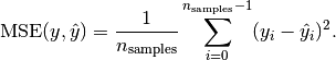
-
MAE: Mean absolute error
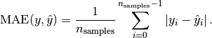
-
rsquared: coefficient of determination
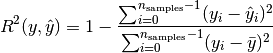
-
explained_variance
-
fscore
(1 + beta˄2) * precison * recall / (beta˄2 * precision + recall)
beta equals 1 by default
-
auc_roc: AUC of ROC using the specified number of bins, by default 100
-
auc_prc: AUC of PRC using the specified number of bins, by default 100
-
counts: Shortcut that resolves to four other metrics: TP, FP, TN, and FN
-
count: Valid only in JSON syntax, counts the number of cases labeled by one class (case-class-label) but predicted as another class (predicted-class-label):
cv_metrics='[{"count":[case-class-label, predicted-class-label]}]'
cv_fold_count- The number of folds to split the data.
Default: 5
cv_hyperparams- A JSON string that describes the combination of parameters for use in grid search of hyper parameters. The JSON string contains pairs of the hyper parameter name. The value of each hyper parameter can be specified as an array or sequence. For example:
{"param1":[value1,value2,...], "param2":{"first":first_value, "step":step_size, "count":number_of_values} }
Hyper parameter names and string values should be quoted using the JSON standard. These parameters are passed to the training function.
cv_prediction_cutoff- The cutoff threshold that is passed to the prediction stage of logistic regression, a FLOAT between 0 and 1, exclusive
Default: 0.5
Model attributes
call_string- The value of all input arguments that were specified at the time
CROSS_VALIDATE was called.
run_average- The average across all folds of all metrics specified in parameter
cv_metrics, if specified; otherwise, average accuracy.
fold_info- The number of rows in each fold:
counters- All counters for the function, including:
-
accepted_row_count: The total number of rows in the input_relation, minus the number of rejected rows.
-
rejected_row_count: The number of rows of the input_relation that were skipped because they contained an invalid value.
-
feature_count: The number of features input to the machine learning model.
run_details- Information about each run, where a run means training a single model, and then testing that model on the one held-out fold:
-
fold_id: The index of the fold held out for testing.
-
iteration_count: The number of iterations used in model training on non-held-out folds.
-
accuracy: All metrics specified in parameter cv_metrics, or accuracy if cv_metrics is not provided.
-
error_rate: All metrics specified in parameter cv_metrics, or accuracy if the parameter is omitted.
Privileges
Non-superusers:
-
SELECT privileges on the input relation
-
CREATE and USAGE privileges on the default schema where machine learning algorithms generate models. If cv_model_name is provided, the cross validation results are saved as a model in the same schema.
Specifying metrics in JSON
Parameter cv_metrics can specify metrics as an array of JSON objects, where each object specifies a metric name . For example, the following expression sets cv_metrics to two metrics specified as JSON objects, accuracy and error_rate:
cv_metrics='["accuracy", "error_rate"]'
In the next example, cv_metrics is set to two metrics, accuracy and TPR (true positive rate). Here, the TPR metric is specified as a JSON object that takes an array of two class label arguments, 2 and 3:
cv_metrics='[ "accuracy", {"TPR":[2,3] } ]'
Metrics specified as JSON objects can accept parameters. In the following example, the fscore metric specifies parameter beta, which is set to 0.5:
cv_metrics='[ {"fscore":{"beta":0.5} } ]'
Parameter support can be especially useful for certain metrics. For example, metrics auc_roc and auc_prc build a curve, and then compute the area under that curve. For ROC, the curve is formed by plotting metrics TPR against FPR; for PRC, PPV (precision) against TPR (recall). The accuracy of such curves can be increased by setting parameter num_bins to a value greater than the default value of 100. For example, the following expression computes AUC for an ROC curve built with 1000 bins:
cv_metrics='[{"auc_roc":{"num_bins":1000}}]'
Using metrics with Multi-class classifier functions
All supported metrics are defined for binary classifier functions
LOGISTIC_REG and
SVM_CLASSIFIER. For multi-class classifier functions such as
NAIVE_BAYES, these metrics can be calculated for each one-versus-the-rest binary classifier. Use arguments to request the metrics for each classifier. For example, if training data has integer class labels, you can set cv_metrics with the precision (PPV) metric as follows:
cv_metrics='[{"precision":[0,4]}]'
This setting specifies to return two columns with precision computed for two classifiers:
If you omit class label arguments, the class with index 1 is used. Instead of computing metrics for individual one-versus-the-rest classifiers, the average is computed in one of the following styles: macro, micro, or weighted (default). For example, the following cv_metrics setting returns the average weighted by class sizes:
cv_metrics='[{"precision":{"avg":"weighted"}}]'
AUC-type metrics can be similarly defined for multi-class classifiers. For example, the following cv_metrics setting computes the area under the ROC curve for each one-versus-the-rest classifier, and then returns the average weighted by class sizes.
cv_metrics='[{"auc_roc":{"avg":"weighted", "num_bins":1000}}]'
Examples
=> SELECT CROSS_VALIDATE('svm_classifier', 'mtcars', 'am', 'mpg'
USING PARAMETERS cv_fold_count= 6,
cv_hyperparams='{"C":[1,5]}',
cv_model_name='cv_svm',
cv_metrics='accuracy, error_rate');
CROSS_VALIDATE
----------------------------
Finished
===========
run_average
===========
C |accuracy |error_rate
---+--------------+----------
1 | 0.75556 | 0.24444
5 | 0.78333 | 0.21667
(1 row)
12.3.3 - ERROR_RATE
Using an input table, returns a table that calculates the rate of incorrect classifications and displays them as FLOAT values.
Using an input table, returns a table that calculates the rate of incorrect classifications and displays them as FLOAT values. ERROR_RATE returns a table with the following dimensions:
Syntax
ERROR_RATE ( targets, predictions [ USING PARAMETERS num_classes = num-classes ] ) OVER()
Arguments
targets- An input column that contains the true values of the response variable.
predictions- An input column that contains the predicted class labels.
Arguments targets and predictions must be set to input columns of the same data type, one of the following: INTEGER, BOOLEAN, or CHAR/VARCHAR. Depending on their data type, these columns identify classes as follows:
-
INTEGER: Zero-based consecutive integers between 0 and (num-classes-1) inclusive, where num-classes is the number of classes. For example, given the following input column values— {0, 1, 2, 3, 4}—Vertica assumes five classes.
Note
If input column values are not consecutive, Vertica interpolates the missing values. Thus, given the following input values— {0, 1, 3, 5, 6,}— Vertica assumes seven classes.
-
BOOLEAN: Yes or No
-
CHAR/VARCHAR: Class names. If the input columns are of type CHAR/VARCHAR columns, you must also set parameter num_classes to the number of classes.
Note
Vertica computes the number of classes as the union of values in both input columns. For example, given the following sets of values in the targets and predictions input columns, Vertica counts four classes:
{'milk', 'soy milk', 'cream'}
{'soy milk', 'almond milk'}
Parameters
num_classesAn integer > 1, specifies the number of classes to pass to the function.
You must set this parameter if the specified input columns are of type CHAR/VARCHAR. Otherwise, the function processes this parameter according to the column data types:
-
INTEGER: By default set to 2, you must set this parameter correctly if the number of classes is any other value.
-
BOOLEAN: By default set to 2, cannot be set to any other value.
Privileges
Non-superusers: model owner, or USAGE privileges on the model
Examples
This example shows how to execute the ERROR_RATE function on an input table named mtcars. The response variables appear in the column obs, while the prediction variables appear in the column pred. Because this example is a classification problem, all response variable values and prediction variable values are either 0 or 1, indicating binary classification.
In the table returned by the function, the first column displays the class id column. The second column displays the corresponding error rate for the class id. The third column indicates how many rows were successfully used by the function and whether any rows were ignored.
=> SELECT ERROR_RATE(obs::int, pred::int USING PARAMETERS num_classes=2) OVER()
FROM (SELECT am AS obs, PREDICT_LOGISTIC_REG (mpg, cyl, disp, drat, wt, qsec, vs, gear, carb
USING PARAMETERS model_name='myLogisticRegModel', type='response') AS pred
FROM mtcars) AS prediction_output;
class | error_rate | comment
-------+--------------------+---------------------------------------------
0 | 0 |
1 | 0.0769230797886848 |
| 0.03125 | Of 32 rows, 32 were used and 0 were ignored
(3 rows)
12.3.4 - LIFT_TABLE
Returns a table that compares the predictive quality of a machine learning model.
Returns a table that compares the predictive quality of a machine learning model. This function is also known as a lift chart.
Syntax
LIFT_TABLE ( targets, probabilities
[ USING PARAMETERS [num_bins = num-bins] [, main_class = class-name ] ] )
OVER()
Arguments
targets- An input column that contains the true values of the response variable, one of the following data types: INTEGER, BOOLEAN, or CHAR/VARCHAR. Depending on the column data type, the function processes column data as follows:
-
INTEGER: Uses the input column as containing the true value of the response variable.
-
BOOLEAN: Resolves Yes to 1, 0 to No.
-
CHAR/VARCHAR: Resolves the value specified by parameter main_class to 1, all other values to 0.
Note
If the input column is of data type INTEGER or BOOLEAN, the function ignores parameter main_class.
probabilities- A FLOAT input column that contains the predicted probability of response being the main class, set to 1 if
targets is of type INTEGER.
Parameters
num_binsAn integer value that determines the number of decision boundaries. Decision boundaries are set at equally spaced intervals between 0 and 1, inclusive. The function computes the table at each num-bin + 1 point.
Default: 100
main_classUsed only if targets is of type CHAR/VARCHAR, specifies the class to associate with the probabilities argument.
Examples
Execute LIFT_TABLE on an input table mtcars.
=> SELECT LIFT_TABLE(obs::int, prob::float USING PARAMETERS num_bins=2) OVER()
FROM (SELECT am AS obs, PREDICT_LOGISTIC_REG(mpg, cyl, disp, drat, wt, qsec, vs, gear, carb
USING PARAMETERS model_name='myLogisticRegModel',
type='probability') AS prob
FROM mtcars) AS prediction_output;
decision_boundary | positive_prediction_ratio | lift | comment
-------------------+---------------------------+------------------+---------------------------------------------
1 | 0 | NaN |
0.5 | 0.40625 | 2.46153846153846 |
0 | 1 | 1 | Of 32 rows, 32 were used and 0 were ignored
(3 rows)
The first column, decision_boundary, indicates the cut-off point for whether to classify a response as 0 or 1. For instance, for each row, if prob is greater than or equal to decision_boundary, the response is classified as 1. If prob is less than decision_boundary, the response is classified as 0.
The second column, positive_prediction_ratio, shows the percentage of samples in class 1 that the function classified correctly using the corresponding decision_boundary value.
For the third column, lift, the function divides the positive_prediction_ratio by the percentage of rows correctly or incorrectly classified as class 1.
12.3.5 - MSE
Returns a table that displays the mean squared error of the prediction and response columns in a machine learning model.
Returns a table that displays the mean squared error of the prediction and response columns in a machine learning model.
Syntax
MSE ( targets, predictions ) OVER()
Arguments
targets- The model response variable, of type FLOAT.
predictions- A FLOAT input column that contains predicted values for the response variable.
Examples
Execute the MSE function on input table faithful_testing. The response variables appear in the column obs, while the prediction variables appear in the column prediction.
=> SELECT MSE(obs, prediction) OVER()
FROM (SELECT eruptions AS obs,
PREDICT_LINEAR_REG (waiting USING PARAMETERS model_name='myLinearRegModel') AS prediction
FROM faithful_testing) AS prediction_output;
mse | Comments
-------------------+-----------------------------------------------
0.252925741352641 | Of 110 rows, 110 were used and 0 were ignored
(1 row)
12.3.6 - PRC
Returns a table that displays the points on a receiver precision recall (PR) curve.
Returns a table that displays the points on a receiver precision recall (PR) curve.
Syntax
PRC ( targets, probabilities
[ USING PARAMETERS
[num_bins = num-bins]
[, f1_score = return-score ]
[, main_class = class-name ] )
OVER()
Arguments
targets- An input column that contains the true values of the response variable, one of the following data types: INTEGER, BOOLEAN, or CHAR/VARCHAR. Depending on the column data type, the function processes column data as follows:
-
INTEGER: Uses the input column as containing the true value of the response variable.
-
BOOLEAN: Resolves Yes to 1, 0 to No.
-
CHAR/VARCHAR: Resolves the value specified by parameter main_class to 1, all other values to 0.
Note
If the input column is of data type INTEGER or BOOLEAN, the function ignores parameter main_class.
probabilities- A FLOAT input column that contains the predicted probability of response being the main class, set to 1 if
targets is of type INTEGER.
Parameters
num_binsAn integer value that determines the number of decision boundaries. Decision boundaries are set at equally spaced intervals between 0 and 1, inclusive. The function computes the table at each num-bin + 1 point.
Default: 100
f1_score- A Boolean that specifies whether to return a column that contains the f1 score—the harmonic average of the precision and recall measures, where an F1 score reaches its best value at 1 (perfect precision and recall) and worst at 0.
Default: false
main_classUsed only if targets is of type CHAR/VARCHAR, specifies the class to associate with the probabilities argument.
Examples
Execute the PRC function on an input table named mtcars. The response variables appear in the column obs, while the prediction variables appear in column pred.
=> SELECT PRC(obs::int, prob::float USING PARAMETERS num_bins=2, f1_score=true) OVER()
FROM (SELECT am AS obs,
PREDICT_LOGISTIC_REG (mpg, cyl, disp, drat, wt, qsec, vs, gear, carb
USING PARAMETERS model_name='myLogisticRegModel',
type='probability') AS prob
FROM mtcars) AS prediction_output;
decision_boundary | recall | precision | f1_score | comment
------------------+--------+-----------+-------------------+--------------------------------------------
0 | 1 | 0.40625 | 0.577777777777778 |
0.5 | 1 | 1 | 1 | Of 32 rows, 32 were used and 0 were ignored
(2 rows)
The first column, decision_boundary, indicates the cut-off point for whether to classify a response as 0 or 1. For example, in each row, if the probability is equal to or greater than decision_boundary, the response is classified as 1. If the probability is less than decision_boundary, the response is classified as 0.
12.3.7 - READ_TREE
Reads the contents of trees within the random forest or XGBoost model.
Reads the contents of trees within the random forest or XGBoost model.
Syntax
READ_TREE ( USING PARAMETERS model_name = 'model-name' [, tree_id = tree-id] [, format = 'format'] )
Parameters
model_name- Identifies the model that is stored as a result of training, where
model-name conforms to conventions described in Identifiers. It must also be unique among all names of sequences, tables, projections, views, and models within the same schema.
tree_id- The tree identifier, an integer between 0 and
n-1, where n is the number of trees in the random forest or XGBoost model. If you omit this parameter, all trees are returned.
format- Output format of the returned tree, one of the following:
Privileges
Non-superusers: USAGE privileges on the model
Examples
Get tabular output from READ_TREE for a random forest model:
=> SELECT READ_TREE ( USING PARAMETERS model_name='myRFModel', tree_id=1 ,
format= 'tabular') LIMIT 2;
-[ RECORD 1 ]-------------+-------------------
tree_id | 1
node_id | 1
node_depth | 0
is_leaf | f
is_categorical_split | f
split_predictor | petal_length
split_value | 1.921875
weighted_information_gain | 0.111242236024845
left_child_id | 2
right_child_id | 3
prediction |
probability/variance |
-[ RECORD 2 ]-------------+-------------------
tree_id | 1
node_id | 2
node_depth | 1
is_leaf | t
is_categorical_split |
split_predictor |
split_value |
weighted_information_gain |
left_child_id |
right_child_id |
prediction | setosa
probability/variance | 1
Get graphviz-formatted output from READ_TREE:
=> SELECT READ_TREE ( USING PARAMETERS model_name='myRFModel', tree_id=1 ,
format= 'graphviz')LIMIT 1;
-[ RECORD 1 ]+-------------------------------------------------------------------
---------------------------------------------------------------------------------
tree_id | 1
tree_digraph | digraph Tree{
1 [label="petal_length < 1.921875 ?", color="blue"];
1 -> 2 [label="yes", color="black"];
1 -> 3 [label="no", color="black"];
2 [label="prediction: setosa, probability: 1", color="red"];
3 [label="petal_length < 4.871875 ?", color="blue"];
3 -> 6 [label="yes", color="black"];
3 -> 7 [label="no", color="black"];
6 [label="prediction: versicolor, probability: 1", color="red"];
7 [label="prediction: virginica, probability: 1", color="red"];
}
This renders as follows:
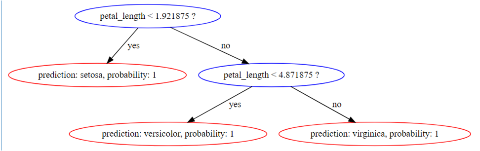
See also
12.3.8 - RF_PREDICTOR_IMPORTANCE
Measures the importance of the predictors in a random forest model using the Mean Decrease Impurity (MDI) approach.
Measures the importance of the predictors in a random forest model using the Mean Decrease Impurity (MDI) approach. The importance vector is normalized to sum to 1.
Syntax
RF_PREDICTOR_IMPORTANCE ( USING PARAMETERS model_name = 'model-name' [, tree_id = tree-id] )
Parameters
model_name- Identifies the model that is stored as a result of the training, where
model-name must be of type rf_classifier or rf_regressor.
tree_id- Identifies the tree to process, an integer between 0 and
n-1, where n is the number of trees in the forest. If you omit this parameter, the function uses all trees to measure importance values.
Privileges
Non-superusers: USAGE privileges on the model
Examples
This example shows how you can use the RF_PREDICTOR_IMPORTANCE function.
=> SELECT RF_PREDICTOR_IMPORTANCE ( USING PARAMETERS model_name = 'myRFModel');
predictor_index | predictor_name | importance_value
-----------------+----------------+--------------------
0 | sepal.length | 0.106763318092655
1 | sepal.width | 0.0279536658041994
2 | petal.length | 0.499198722346586
3 | petal.width | 0.366084293756561
(4 rows)
See also
12.3.9 - ROC
Returns a table that displays the points on a receiver operating characteristic curve.
Returns a table that displays the points on a receiver operating characteristic curve. The ROC function tells you the accuracy of a classification model as you raise the discrimination threshold for the model.
Syntax
ROC ( targets, probabilities
[ USING PARAMETERS
[num_bins = num-bins]
[, AUC = output]
[, main_class = class-name ] ) ] )
OVER()
Arguments
targets- An input column that contains the true values of the response variable, one of the following data types: INTEGER, BOOLEAN, or CHAR/VARCHAR. Depending on the column data type, the function processes column data as follows:
-
INTEGER: Uses the input column as containing the true value of the response variable.
-
BOOLEAN: Resolves Yes to 1, 0 to No.
-
CHAR/VARCHAR: Resolves the value specified by parameter main_class to 1, all other values to 0.
Note
If the input column is of data type INTEGER or BOOLEAN, the function ignores parameter main_class.
probabilities- A FLOAT input column that contains the predicted probability of response being the main class, set to 1 if
targets is of type INTEGER.
Parameters
num_binsAn integer value that determines the number of decision boundaries. Decision boundaries are set at equally spaced intervals between 0 and 1, inclusive. The function computes the table at each num-bin + 1 point.
Default: 100
Greater values result in more precise approximations of the AUC.
AUC- A Boolean value that specifies whether to output the area under the curve (AUC) value.
Default: True
main_classUsed only if targets is of type CHAR/VARCHAR, specifies the class to associate with the probabilities argument.
Examples
Execute ROC on input table mtcars. Observed class labels are in column obs, predicted class labels are in column prob:
=> SELECT ROC(obs::int, prob::float USING PARAMETERS num_bins=5, AUC = True) OVER()
FROM (SELECT am AS obs,
PREDICT_LOGISTIC_REG (mpg, cyl, disp, drat, wt, qsec, vs, gear, carb
USING PARAMETERS
model_name='myLogisticRegModel', type='probability') AS prob
FROM mtcars) AS prediction_output;
decision_boundary | false_positive_rate | true_positive_rate | AUC |comment
-------------------+---------------------+--------------------+-----+-----------------------------------
0 | 1 | 1 | |
0.5 | 0 | 1 | |
1 | 0 | 0 | 1 | Of 32 rows,32 were used and 0 were ignoreded
(3 rows)
The function returns a table with the following results:
-
decision_boundary indicates the cut-off point for whether to classify a response as 0 or 1. In each row, if prob is equal to or greater than decision_boundary, the response is classified as 1. If prob is less than decision_boundary, the response is classified as 0.
-
false_positive_rate shows the percentage of false positives (when 0 is classified as 1) in the corresponding decision_boundary.
-
true_positive_rate shows the percentage of rows that were classified as 1 and also belong to class 1.
12.3.10 - RSQUARED
Returns a table with the R-squared value of the predictions in a regression model.
Returns a table with the R-squared value of the predictions in a regression model.
Syntax
RSQUARED ( targets, predictions ) OVER()
Important
The OVER() clause must be empty.
Arguments
targets- A FLOAT response variable for the model.
predictions- A FLOAT input column that contains the predicted values for the response variable.
Examples
This example shows how to execute the RSQUARED function on an input table named faithful_testing. The observed values of the response variable appear in the column, obs, while the predicted values of the response variable appear in the column, pred.
=> SELECT RSQUARED(obs, prediction) OVER()
FROM (SELECT eruptions AS obs,
PREDICT_LINEAR_REG (waiting
USING PARAMETERS model_name='myLinearRegModel') AS prediction
FROM faithful_testing) AS prediction_output;
rsq | comment
-------------------+-----------------------------------------------
0.801392981147911 | Of 110 rows, 110 were used and 0 were ignored
(1 row)
12.3.11 - XGB_PREDICTOR_IMPORTANCE
Measures the importance of the predictors in an XGBoost model.
Measures the importance of the predictors in an XGBoost model. The function outputs three measures of importance for each predictor:
-
frequency: relative number of times the model uses a predictor to split the data.
-
total_gain: relative contribution of a predictor to the model based on the total information gain across a predictor's splits. A higher value means more predictive importance.
-
avg_gain: relative contribution of a predictor to the model based on the average information gain across a predictor's splits.
The sum of each importance measure is normalized to one across all predictors.
Syntax
XGB_PREDICTOR_IMPORTANCE ( USING PARAMETERS param=value[,...] )
Parameters
model_name- Name of the model, which must be of type
xgb_classifier or xgb_regressor.
tree_id- Integer in the range [0,
n-1], where n is the number of trees in model_name, that specifies the tree to process. If you omit this parameter, the function uses all trees in the model to measure predictor importance values.
Privileges
Non-superusers: USAGE privileges on the model
Examples
The following example measures the importance of the predictors in the model 'xgb_iris', an XGBoost classifier model, across all trees:
=> SELECT XGB_PREDICTOR_IMPORTANCE( USING PARAMETERS model_name = 'xgb_iris' );
predictor_index | predictor_name | frequency | total_gain | avg_gain
-----------------+----------------+-------------------+--------------------+--------------------
0 | sepal_length | 0.15384615957737 | 0.0183021749937 | 0.0370849960701401
1 | sepal_width | 0.215384617447853 | 0.0154729501420881 | 0.0223944615251752
2 | petal_length | 0.369230777025223 | 0.607349886817728 | 0.512770753876444
3 | petal_width | 0.261538475751877 | 0.358874988046484 | 0.427749788528241
(4 rows)
To sort the predictors by importance values, you can use a nested query with an ORDER BY clause. The following sorts the model predictors by descending avg_gain:
=> SELECT * FROM (SELECT XGB_PREDICTOR_IMPORTANCE( USING PARAMETERS model_name = 'xgb_iris' )) AS importances ORDER BY avg_gain DESC;
predictor_index | predictor_name | frequency | total_gain | avg_gain
-----------------+----------------+-------------------+--------------------+--------------------
2 | petal_length | 0.369230777025223 | 0.607349886817728 | 0.512770753876444
3 | petal_width | 0.261538475751877 | 0.358874988046484 | 0.427749788528241
0 | sepal_length | 0.15384615957737 | 0.0183021749937 | 0.0370849960701401
1 | sepal_width | 0.215384617447853 | 0.0154729501420881 | 0.0223944615251752
(4 rows)
See also
12.4 - Model management
Vertica provides several functions for managing models.
Vertica provides several functions for managing models.
12.4.1 - CHANGE_MODEL_STATUS
Changes the status of a registered model.
Changes the status of a registered model. Only dbadmin and users with the MLSUPERVISOR role can call this function.
The following diagram depicts the valid status transitions:
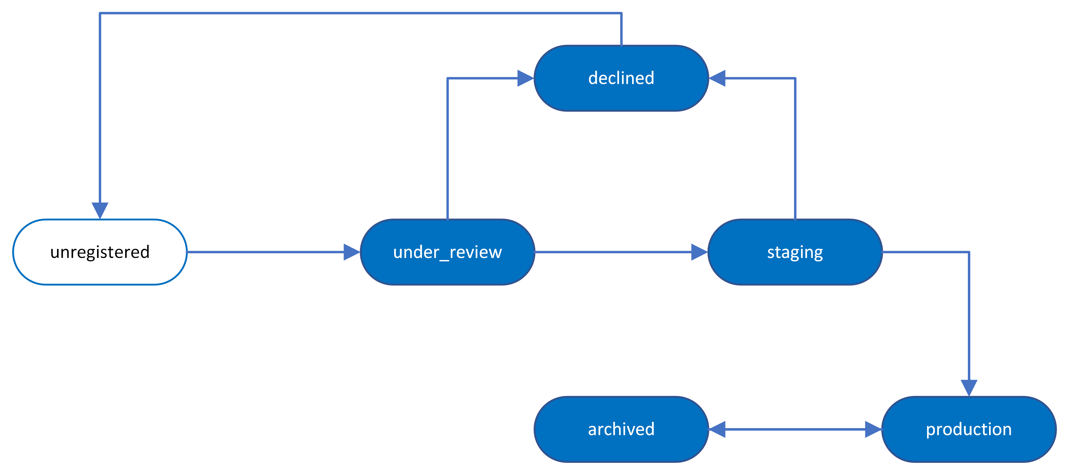
This is a meta-function. You must call meta-functions in a top-level SELECT statement.
Behavior type
Stable
Syntax
CHANGE_MODEL_STATUS( 'registered_name', registered_version, 'new_status' )
Arguments
registered_name- Identifies the abstract name to which the model is registered. This
registered_name can represent a group of models for a higher-level application, where each model in the group has a unique version number.
registered_version- Unique version number of the model under the specified
registered_name.
If there is no registered model with the given registered_name and registered_version, the function errors.
new_status- New status of the registered model. Must be one of the following strings and adhere to the valid status transitions depicted in the above diagram:
-
under_review: Status assigned to newly registered models.
-
staging: Model is targeted for A/B testing against the model currently in production.
-
production: Model is in production for its specified application. Only one model can be in production for a given registered_name at one time.
-
archived: Status of models that were previously in production. Archived models can be returned to production at any time.
-
declined: Model is no longer in consideration for production.
-
unregistered: Model is removed from the versioning environment. The model does not appear in the REGISTERED_MODELS system table.
If you change the status of a model to 'production' and there is already a model in production under the given registered_name, the status of the model in production is set to 'archived' and the status of the new model is set to 'production'.
Privileges
One of the following:
Examples
In the following example, the linear_reg_spark1 model, which is uniquely identified by the registered_name 'linear_reg_app' and the registered_version of two, is set to 'production' status:
=> SELECT * FROM REGISTERED_MODELS;
registered_name | registered_version | status | registered_time | model_id | schema_name | model_name | model_type | category
------------------+--------------------+--------------+-------------------------------+-------------------+-------------+-------------------+-----------------------+----------------
linear_reg_app | 2 | STAGING | 2023-01-29 05:49:00.082166-04 | 45035996273714020 | public | linear_reg_spark1 | PMML_REGRESSION_MODEL | PMML
linear_reg_app | 1 | PRODUCTION | 2023-01-24 09:19:04.553102-05 | 45035996273850350 | public | native_linear_reg | LINEAR_REGRESSION | VERTICA_MODELS
logistic_reg_app | 1 | DECLINED | 2023-01-11 02:47:25.990626-02 | 45035996273853740 | public | log_reg_bfgs | LOGISTIC_REGRESSION | VERTICA_MODELS
(3 rows)
=> SELECT CHANGE_MODEL_STATUS('linear_reg_app', 2, 'production');
CHANGE_MODEL_STATUS
-----------------------------------------------------------------------------
The status of model [linear_reg_app] - version [2] is changed to [production]
(1 row)
You can query the REGISTERED_MODELS system table to confirm that the linear_reg_spark1 model is now in 'production' and the native_linear_reg model, which was currently in 'production', is moved to 'archived':
=> SELECT * FROM REGISTERED_MODELS;
registered_name | registered_version | status | registered_time | model_id | schema_name | model_name | model_type | category
------------------+--------------------+--------------+-------------------------------+-------------------+-------------+-------------------+-----------------------+----------------
linear_reg_app | 2 | PRODUCTION | 2023-01-29 05:49:00.082166-04 | 45035996273714020 | public | linear_reg_spark1 | PMML_REGRESSION_MODEL | PMML
linear_reg_app | 1 | ARCHIVED | 2023-01-24 09:19:04.553102-05 | 45035996273850350 | public | native_linear_reg | LINEAR_REGRESSION | VERTICA_MODELS
logistic_reg_app | 1 | DECLINED | 2023-01-11 02:47:25.990626-02 | 45035996273853740 | public | log_reg_bfgs | LOGISTIC_REGRESSION | VERTICA_MODELS
(2 rows)
If you change a model's status to 'unregistered', the model is removed from the model versioning environment and no longer appears in the REGISTERED_MODELS system table:
=> SELECT CHANGE_MODEL_STATUS('logistic_reg_app', 1, 'unregistered');
CHANGE_MODEL_STATUS
----------------------------------------------------------------------------------
The status of model [logistic_reg_app] - version [1] is changed to [unregistered]
(1 row)
=> SELECT * FROM REGISTERED_MODELS;
registered_name | registered_version | status | registered_time | model_id | schema_name | model_name | model_type | category
------------------+--------------------+--------------+-------------------------------+-------------------+-------------+-------------------+-----------------------+----------------
linear_reg_app | 2 | STAGING | 2023-01-29 05:49:00.082166-04 | 45035996273714020 | public | linear_reg_spark1 | PMML_REGRESSION_MODEL | PMML
linear_reg_app | 1 | PRODUCTION | 2023-01-24 09:19:04.553102-05 | 45035996273850350 | public | native_linear_reg | LINEAR_REGRESSION | VERTICA_MODELS
(2 rows)
See also
12.4.2 - EXPORT_MODELS
Exports machine learning models.
Exports machine learning models. Vertica supports three model formats:
This is a meta-function. You must call meta-functions in a top-level SELECT statement.
Behavior type
Volatile
Syntax
EXPORT_MODELS ( 'output-dir', 'export-target' [ USING PARAMETERS category = 'model-category' ] )
Arguments
output-dir- Absolute path of an output directory to store the exported models, either an absolute path on the initiator node file system or a URI for a supported file system or object store.
export-target- Models to export:
[schema.]{model-name | * }
schema specifies the schema from which models are exported. If omitted, EXPORT_MODELS uses the default schema. Supply * (asterisk) to batch export all models from the schema.
If a model in a batch fails to export, the function issues a warning and then continues to export any remaining models in the batch. Details about any failed model exports are available in the log file generated at the output-dir location.
Parameters
category- The category of models to export, one of the following:
-
VERTICA_MODELS
-
PMML
-
TENSORFLOW
EXPORT_MODELS exports models of the specified category according to the scope of the export operation—that is, whether it applies to a single model, or to all models within a schema. See Export Scope and Category Processing below.
Exported Files below describes the files that EXPORT_MODELS exports for each category.
If you omit this parameter, EXPORT_MODELS exports the model, or models in the specified schema, according to their model type.
Privileges
Superuser or MLSUPERVISOR
Export scope and category processing
EXPORT_MODELS executes according to the following parameter settings:
-
Scope of the export operation: single model, or all models within a given schema
-
Category specified or omitted
The following table shows how these two parameters control the export process:
|
Export scope |
If category specified... |
If category omitted... |
|
Single model |
Convert the model to the specified category, provided the model and category are compatible; otherwise, return with a mismatch error. |
Export the model according to model type. |
|
All models in schema |
Export only models that are compatible with the specified category and issue mismatch warnings on all other models in the schema. |
Export all models in the schema according to model type. |
Exported files
EXPORT_MODELS exports the following files for each model category:
VERTICA_MODELS
-
Multiple binary files (exact number dependent on model type)
-
metadata.json: Metadata file with model information, including model name, category, type, and Vertica version on export.
-
crc.json: Used on import to validate other files of this model.
PMML
-
XML file with the same name as the model and complying with PMML standard.
-
metadata.json: Metadata file with model information, including model name, category, type, and Vertica version on export.
-
crc.json: Used on import to validate other files of this model.
TENSORFLOW
-
model-name.pb: Contains the TensorFlow model, saved in 'frozen graph' format.
-
metadata.json: Metadata file with model information, including model name, category, type, and Vertica version on export.
-
tf_model_desc.json: Summary model description.
-
model.json: Verbose model description.
-
crc.json: Used on import to validate other files of this model.
Categories and compatible models
If EXPORT_MODELS specifies a single model and also sets the category parameter, the function succeeds if the model type and category are compatible; otherwise, it returns with an error. The following model types are compatible with the listed categories:
PMMLPMMLTensorFlowTENSORFLOWVERTICA_MODELSPMML
VERTICA_MODELS
If EXPORT_MODELS specifies to export all models from a schema and sets a category, it issues a warning message on each model that is incompatible with that category. The function then continues to process remaining models in that schema.
EXPORT_MODELS logs all errors and warnings in output-dir/export_log.json.
Examples
Export models without changing their category
Export model myschema.mykmeansmodel without changing its category:
=> SELECT EXPORT_MODELS ('/home/dbadmin', 'myschema.mykmeansmodel');
EXPORT_MODELS
----------------
Success
(1 row)
Export all models in schema myschema without changing their categories:
=> SELECT EXPORT_MODELS ('/home/dbadmin', 'myschema.*');
EXPORT_MODELS
----------------
Success
(1 row)
Export all the models in schema models to an S3 bucket without changing the model categories:
SELECT export_models('s3://vertica/ml_models', 'models.*');
EXPORT_MODELS
---------------
Success
(1 row)
Export models that are compatible with the specified category
Note
When you import a model of category VERTICA_MODELS trained in a different version of Vertica, Vertica automatically upgrades the model version to match that of the database. If this fails, you must run UPGRADE_MODEL.
If both methods fail, the model cannot be used for in-database scoring and cannot be exported as a PMML model.
The category is set to PMML. Models of type PMML and VERTICA_MODELS are compatible with the PMML category, so the export operation succeeds if my_keans is of either type:
=> SELECT EXPORT_MODELS ('/tmp/', 'my_kmeans' USING PARAMETERS category='PMML');
The category is set to VERTICA_MODELS. Only models of type VERTICA_MODELS are compatible with the VERTICA_MODELS category, so the export operation succeeds only if my_keans is of that type:
=> SELECT EXPORT_MODELS ('/tmp/', 'public.my_kmeans' USING PARAMETERS category='VERTICA_MODELS');
The category is set to TENSORFLOW. Only models of type TensorFlow are compatible with the TENSORFLOW category, so the model tf_mnist_keras must be of type TensorFlow:
=> SELECT EXPORT_MODELS ('/tmp/', 'tf_mnist_keras', USING PARAMETERS category='TENSORFLOW');
export_models
---------------
Success
(1 row)
After exporting the TensorFlow model tf_mnist_keras, list the exported files:
$ ls tf_mnist_keras/
crc.json metadata.json mnist_keras.pb model.json tf_model_desc.json
See also
IMPORT_MODELS
12.4.3 - GET_MODEL_ATTRIBUTE
Extracts either a specific attribute from a model or all attributes from a model.
Extracts either a specific attribute from a model or all attributes from a model. Use this function to view a list of attributes and row counts or view detailed information about a single attribute. The output of GET_MODEL_ATTRIBUTE is a table format where users can select particular columns or rows.
Syntax
GET_MODEL_ATTRIBUTE ( USING PARAMETERS model_name = 'model-name' [, attr_name = 'attribute' ] )
Parameters
model_nameName of the model (case-insensitive).
attr_name- Name of the model attribute to extract. If omitted, the function shows all available attributes. Attribute names are case-sensitive.
Privileges
Non-superusers: model owner, or USAGE privileges on the model
Examples
This example returns a summary of all model attributes.
=> SELECT GET_MODEL_ATTRIBUTE ( USING PARAMETERS model_name='myLinearRegModel');
attr_name | attr_fields | #_of_rows
-------------------+---------------------------------------------------+-----------
details | predictor, coefficient, std_err, t_value, p_value | 2
regularization | type, lambda | 1
iteration_count | iteration_count | 1
rejected_row_count | rejected_row_count | 1
accepted_row_count | accepted_row_count | 1
call_string | call_string | 1
(6 rows)
This example extracts the details attribute from the myLinearRegModel model.
=> SELECT GET_MODEL_ATTRIBUTE ( USING PARAMETERS model_name='myLinearRegModel', attr_name='details');
coeffNames | coeff | stdErr | zValue | pValue
-----------+--------------------+---------------------+-------------------+-----------------------
Intercept | -1.87401598641074 | 0.160143331525544 | -11.7021169008952 | 7.3592939615234e-26
waiting | 0.0756279479518627 | 0.00221854185633525 | 34.0890336307608 | 8.13028381124448e-100
(2 rows)
12.4.4 - GET_MODEL_SUMMARY
Returns summary information of a model.
Returns summary information of a model.
Syntax
GET_MODEL_SUMMARY ( USING PARAMETERS model_name = 'model-name' )
Parameters
- model_name
Name of the model (case-insensitive).
Privileges
Non-superusers: model owner, or USAGE privileges on the model
Examples
This example shows how you can view the summary of a linear regression model.
=> SELECT GET_MODEL_SUMMARY( USING PARAMETERS model_name='myLinearRegModel');
--------------------------------------------------------------------------------
=======
details
=======
predictor|coefficient|std_err |t_value |p_value
---------+-----------+--------+--------+--------
Intercept| -2.06795 | 0.21063|-9.81782| 0.00000
waiting | 0.07876 | 0.00292|26.96925| 0.00000
==============
regularization
==============
type| lambda
----+--------
none| 1.00000
===========
call_string
===========
linear_reg('public.linear_reg_faithful', 'faithful_training', '"eruptions"', 'waiting'
USING PARAMETERS optimizer='bfgs', epsilon=1e-06, max_iterations=100,
regularization='none', lambda=1)
===============
Additional Info
===============
Name |Value
------------------+-----
iteration_count | 3
rejected_row_count| 0
accepted_row_count| 162
(1 row)
12.4.5 - IMPORT_MODELS
Imports models into Vertica, either Vertica models that were exported with EXPORT_MODELS, or models in Predictive Model Markup Language (PMML) or TensorFlow format.
Imports models into Vertica, either Vertica models that were exported with EXPORT_MODELS, or models in Predictive Model Markup Language (PMML) or TensorFlow format. You can use this function to move models between Vertica clusters, or to import PMML and TensorFlow models trained elsewhere.
Other Vertica model management operations such as GET_MODEL_SUMMARY and GET_MODEL_ATTRIBUTE support imported models.
Caution
Changing the exported model files causes the import functionality to fail on attempted re-import.
This is a meta-function. You must call meta-functions in a top-level SELECT statement.
Behavior type
Volatile
Syntax
IMPORT_MODELS ( 'source'
[ USING PARAMETERS [ new_schema = 'schema-name' ] [, category = 'model-category' ] ] )
Arguments
source- Path from which to import models, either an absolute path on the initiator node file system or a URI for a supported file system or object store. The path format depends on whether you are importing a single model or a batch of models:
-
To import a single model, provide the path to the model's directory:
path/model-directory
-
To import a batch of models, provide the path to a parent directory that contains the model directories for each model in the batch:
parent-dir-path/*
If a model in a batch fails to import, the function issues a warning and then continues to import any remaining models in the batch. Details about any failed model import are available in the log file generated at the source location.
Parameters
new_schema- An existing schema where the machine learning models are imported. If omitted, models are imported to the default schema.
IMPORT_MODELS extracts the name of the imported model from its metadata.json file, if it exists. Otherwise, the function uses the name of the model directory.
category- Specifies the category of the model to import, one of the following:
-
VERTICA_MODELS
-
PMML
-
TENSORFLOW
This parameter is required if the model directory has no metadata.json file. IMPORT_MODELS returns with an error if one of the following cases is true:
Note
If the category is TENSORFLOW, IMPORT_MODELS only imports the following files from the model directory:
Privileges
Superuser or MLSUPERVISOR
Requirements and restrictions
The following requirements and restrictions apply:
-
If you export a model, then import it again, the export and import model directory names must match. If naming conflicts occur, import the model to a different schema by using the new_schema parameter, and then rename the model.
-
The machine learning configuration parameter MaxModelSizeKB sets the maximum size of a model that can be imported into Vertica.
-
Some PMML features and attributes are not currently supported. See PMML features and attributes for details.
-
If you import a PMML model with both metadata.json and crc.json files, the CRC file must contain the metadata file's CRC value. Otherwise, the import operation returns with an error.
Examples
If no model category is specified, IMPORT_MODELS uses the model's metadata.json file to determine its category.
Import a single model mykmeansmodel into the newschema schema:
=> SELECT IMPORT_MODELS ('/home/dbadmin/myschema/mykmeansmodel' USING PARAMETERS new_schema='newschema')
IMPORT_MODELS
----------------
Success
(1 row)
Import all models in the myschema directory into the newschema schema:
=> SELECT IMPORT_MODELS ('/home/dbadmin/myschema/*' USING PARAMETERS new_schema='newschema')
IMPORT_MODELS
----------------
Success
(1 row)
Import the model tf_mnsit_estimator from an S3 bucket into the ml_models schema:
=> SELECT IMPORT_MODELS ('s3://ml-models/tensorflow/mnist' USING PARAMETERS new_schema='ml_models')
IMPORT MODELS
---------------
Success
(1 row)
When you set the category parameter, the specified category must match the model type of the imported models; otherwise, the function returns an error.
Import kmeans_pmml as a PMML model:
SELECT IMPORT_MODELS ('/root/user/kmeans_pmml' USING PARAMETERS category='PMML')
import_models
---------------
Success
(1 row)
Attempt to import kmeans_pmml, a PMML model, as a TENSORFLOW model:
SELECT IMPORT_MODELS ('/root/user/kmeans_pmml' USING PARAMETERS category='TENSORFLOW')
import_models
-------------------------------------------------
Has failure. Please check import_log.json file
(1 row)
Import tf_mnist_estimator as a TensorFlow model:
=> SELECT IMPORT_MODELS ( '/path/tf_models/tf_mnist_estimator' USING PARAMETERS category='TENSORFLOW');
import_models
---------------
Success
(1 row)
Import all TensorFlow models from the specified directory:
=> SELECT IMPORT_MODELS ( '/path/tf_models/*' USING PARAMETERS category='TENSORFLOW');
import_models
---------------
Success
(1 row)
See also
EXPORT_MODELS
12.4.6 - REGISTER_MODEL
Registers a trained model and adds it to Model Versioning environment with a status of 'under_review'.
Registers a trained model and adds it to Model versioning environment with a status of 'under_review'. The model must be registered by the owner of the model, dbadmin, or MLSUPERVISOR.
After a model is registered, the model owner is automatically changed to Superuser and the previous owner is given USAGE privileges. Users with the MLSUPERVISOR role or dbamin can call the CHANGE_MODEL_STATUS function to alter the status of registered models.
This is a meta-function. You must call meta-functions in a top-level SELECT statement.
Behavior type
Stable
Syntax
REGISTER_MODEL( 'model_name', 'registered_name' )
Arguments
model_name- Identifies the model to register. If the model has already been registered, the function throws an error.
registered_name- Identifies an abstract name to which the model is registered. This
registered_name can represent a group of models for a higher-level application, where each model in the group has a unique version number.
If a model is the first to be registered to a given registered_name, the model is assigned a registered_version of one. Otherwise, newly registered models are assigned an incremented registered_version of n + 1, where n is the number of models already registered to the given registered_name. Each registered model can be uniquely identified by the combination of registered_name and registered_version.
Privileges
Non-superusers: model owner
Examples
In the following example, the model log_reg_bfgs is registered to the logistic_reg_app application:
=> SELECT REGISTER_MODEL('log_reg_bfgs', 'logistic_reg_app');
REGISTER_MODEL
----------------------------------------------------------------------
Model [log_reg_bfgs] is registered as [logistic_reg_app], version [1]
(1 row)
You can query the REGISTERED_MODELS system table to view details about the newly registered model:
=> SELECT * FROM REGISTERED_MODELS;
registered_name | registered_version | status | registered_time | model_id | schema_name | model_name | model_type | category
------------------+--------------------+--------------+-------------------------------+-------------------+-------------+-------------------+-----------------------+----------------
logistic_reg_app | 1 | UNDER_REVIEW | 2023-01-22 09:49:25.990626-02 | 45035996273853740 | public | log_reg_bfgs | LOGISTIC_REGRESSION | VERTICA_MODELS
(1 row)
See also
12.4.7 - UPGRADE_MODEL
Upgrades a model from a previous Vertica version.
Upgrades a model from a previous Vertica version. Vertica automatically runs this function during a database upgrade and if you run the IMPORT_MODELS function. Manually call this function to upgrade models after a backup or restore.
If UPGRADE_MODEL fails to upgrade the model and the model is of category VERTICA_MODELS, it cannot be used for in-database scoring and cannot be exported as a PMML model.
This is a meta-function. You must call meta-functions in a top-level SELECT statement.
Behavior type
Volatile
Syntax
UPGRADE_MODEL ( [ USING PARAMETERS [model_name = 'model-name'] ] )
Parameters
model_name- Name of the model to upgrade. If you omit this parameter, Vertica upgrades all models on which you have privileges.
Privileges
Non-superuser: Upgrades only models that the user owns.
Examples
Upgrade model myLogisticRegModel:
=> SELECT UPGRADE_MODEL( USING PARAMETERS model_name = 'myLogisticRegModel');
UPGRADE_MODEL
----------------------------
1 model(s) upgrade
(1 row)
Upgrade all models that the user owns:
=> SELECT UPGRADE_MODEL();
UPGRADE_MODEL
----------------------------
20 model(s) upgrade
(1 row)
12.5 - Transformation functions
The machine learning API includes a set of UDx functions that transform the columns of each input row to one or more corresponding output columns.
The machine learning API includes a set of UDx functions that transform the columns of each input row to one or more corresponding output columns. These transformations follow rules that are defined in models that were created earlier. For example,
APPLY_SVD uses an SVD model to transform input data.
Unless otherwise indicated, these functions require the following privileges for non-superusers:
In general, given an invalid input row, the return value for these functions is NULL.
12.5.1 - APPLY_BISECTING_KMEANS
Applies a trained bisecting k-means model to an input relation, and assigns each new data point to the closest matching cluster in the trained model.
Applies a trained bisecting k-means model to an input relation, and assigns each new data point to the closest matching cluster in the trained model.
Note
If the input relation is defined in Hive, use
SYNC_WITH_HCATALOG_SCHEMA to sync the
hcatalog schema, and then run the machine learning function.
Syntax
SELECT APPLY_BISECTING_KMEANS( 'input-columns'
USING PARAMETERS model_name = 'model-name'
[, num_clusters = 'num-clusters']
[, match_by_pos = match-by-position] ] )
Arguments
input-columns- Comma-separated list of columns to use from the input relation, or asterisk (*) to select all columns. Input columns must be of data type numeric.
Parameters
model_nameName of the model (case-insensitive).
num_clusters- Integer between 1 and
k inclusive, where k is the number of centers in the model, specifies the number of clusters to use for prediction.
Default: Value that the model specifies for k
match_by_posBoolean value that specifies how input columns are matched to model features:
Privileges
Non-superusers: model owner, or USAGE privileges on the model
12.5.2 - APPLY_IFOREST
Applies an isolation forest (iForest) model to an input relation.
Applies an isolation forest (iForest) model to an input relation. For each input row, the function returns an output row with two fields:
anomaly_score: A float value that represents the average path length across all trees in the model normalized by the training sample size.is_anomaly: A Boolean value that indicates whether the input row is an anomaly. This value is true when anomaly_score is equal to or larger than a given threshold; otherwise, it's false.
Syntax
APPLY_IFOREST( input-columns USING PARAMETERS param=value[,...] )
Arguments
input-columns- Comma-separated list of columns to use from the input relation, or asterisk (*) to select all columns. Column types must match the types of the predictors in
model_name.
Parameters
model_nameName of the model (case-insensitive).
threshold- Optional. Float in the range (0.0, 1.0), specifies the threshold that determines if a data point is an anomaly. If the
anomaly_score for a data point is equal to or larger than the value of threshold, the data point is marked as an outlier.
Alternatively, you can specify a contamination value that sets a threshold where the percentage of training data points labeled as outliers is approximately equal to the value of contamination. You cannot set both contamination and threshold in the same function call.
Default: 0.7
match_by_pos- Optional. Boolean value that specifies how input columns are matched to model columns:
Default: false
contamination- Optional. Float in the range (0.0, 1.0), the approximate ratio of data points in the training data that are labeled as outliers. The function calculates a threshold based on this
contamination value. If you do not set this parameter, the function marks outliers using the specified or default threshold value.
You cannot set both contamination and threshold in the same function call.
Privileges
Non-superusers:
Examples
The following example demonstrates how different threshold values can affect outlier detection on an input relation:
=> SELECT * FROM (SELECT first_name, last_name, APPLY_IFOREST(team, hr, hits, avg, salary USING PARAMETERS model_name='baseball_anomalies',
threshold=0.75) AS predictions FROM baseball) AS outliers WHERE predictions.is_anomaly IS true;
first_name | last_name | predictions
------------+-----------+-------------------------------------------------------
Jacqueline | Richards | {"anomaly_score":0.777757463074347,"is_anomaly":true}
(1 row)
=> SELECT * FROM (SELECT first_name, last_name, APPLY_IFOREST(team, hr, hits, avg, salary USING PARAMETERS model_name='baseball_anomalies',
threshold=0.55) AS predictions FROM baseball) AS outliers WHERE predictions.is_anomaly IS true;
first_name | last_name | predictions
------------+-----------+--------------------------------------------------------
Jacqueline | Richards | {"anomaly_score":0.777757463074347,"is_anomaly":true}
Debra | Hall | {"anomaly_score":0.5714649698133808,"is_anomaly":true}
Gerald | Fuller | {"anomaly_score":0.5980549926114661,"is_anomaly":true}
(3 rows)
You can also use different contamination values to alter the outlier threshold:
=> SELECT * FROM (SELECT first_name, last_name, APPLY_IFOREST(team, hr, hits, avg, salary USING PARAMETERS model_name='baseball_anomalies',
contamination = 0.1) AS predictions FROM baseball) AS outliers WHERE predictions.is_anomaly IS true;
first_name | last_name | predictions
------------+-----------+--------------------------------------------------------
Marie | Fields | {"anomaly_score":0.5307715717521868,"is_anomaly":true}
Jacqueline | Richards | {"anomaly_score":0.777757463074347,"is_anomaly":true}
Debra | Hall | {"anomaly_score":0.5714649698133808,"is_anomaly":true}
Gerald | Fuller | {"anomaly_score":0.5980549926114661,"is_anomaly":true}
(4 rows)
=> SELECT * FROM (SELECT first_name, last_name, APPLY_IFOREST(team, hr, hits, avg, salary USING PARAMETERS model_name='baseball_anomalies',
contamination = 0.01) AS predictions FROM baseball) AS outliers WHERE predictions.is_anomaly IS true;
first_name | last_name | predictions
------------+-----------+--------------------------------------------------------
Jacqueline | Richards | {"anomaly_score":0.777757463074347,"is_anomaly":true}
Debra | Hall | {"anomaly_score":0.5714649698133808,"is_anomaly":true}
Gerald | Fuller | {"anomaly_score":0.5980549926114661,"is_anomaly":true}
(3 rows)
See also
12.5.3 - APPLY_INVERSE_PCA
Inverts the APPLY_PCA-generated transform back to the original coordinate system.
Inverts the APPLY_PCA-generated transform back to the original coordinate system.
Syntax
APPLY_INVERSE_PCA ( input-columns
USING PARAMETERS model_name = 'model-name'
[, exclude_columns = 'excluded-columns']
[, key_columns = 'key-columns'] )
Arguments
input-columns- Comma-separated list of columns to use from the input relation, or asterisk (*) to select all columns. The following requirements apply:
Parameters
model_nameName of the model (case-insensitive).
exclude_columnsComma-separated list of column names from input-columns to exclude from processing.
key_columns- Comma-separated list of column names from
input-columns that identify its data rows. These columns are included in the output table.
Examples
The following example shows how to use the APPLY_INVERSE_PCA function. It shows the output for the first record.
=> SELECT PCA ('pcamodel', 'world','country,HDI,em1970,em1971,em1972,em1973,em1974,em1975,em1976,em1977,
em1978,em1979,em1980,em1981,em1982,em1983,em1984 ,em1985,em1986,em1987,em1988,em1989,em1990,em1991,em1992,
em1993,em1994,em1995,em1996,em1997,em1998,em1999,em2000,em2001,em2002,em2003,em2004,em2005,em2006,em2007,
em2008,em2009,em2010,gdp1970,gdp1971,gdp1972,gdp1973,gdp1974,gdp1975,gdp1976,gdp1977,gdp1978,gdp1979,gdp1980,
gdp1981,gdp1982,gdp1983,gdp1984,gdp1985,gdp1986,gdp1987,gdp1988,gdp1989,gdp1990,gdp1991,gdp1992,gdp1993,
gdp1994,gdp1995,gdp1996,gdp1997,gdp1998,gdp1999,gdp2000,gdp2001,gdp2002,gdp2003,gdp2004,gdp2005,gdp2006,
gdp2007,gdp2008,gdp2009,gdp2010' USING PARAMETERS exclude_columns='HDI,country');
PCA
---------------------------------------------------------------
Finished in 1 iterations.
Accepted Rows: 96 Rejected Rows: 0
(1 row)
=> CREATE TABLE worldPCA AS SELECT
APPLY_PCA (HDI,country,em1970,em1971,em1972,em1973,em1974,em1975,em1976,em1977,em1978,em1979,
em1980,em1981,em1982,em1983,em1984 ,em1985,em1986,em1987,em1988,em1989,em1990,em1991,em1992,em1993,em1994,
em1995,em1996,em1997,em1998,em1999,em2000,em2001,em2002,em2003,em2004,em2005,em2006,em2007,em2008,em2009,
em2010,gdp1970,gdp1971,gdp1972,gdp1973,gdp1974,gdp1975,gdp1976,gdp1977,gdp1978,gdp1979,gdp1980,gdp1981,gdp1982,
gdp1983,gdp1984,gdp1985,gdp1986,gdp1987,gdp1988,gdp1989,gdp1990,gdp1991,gdp1992,gdp1993,gdp1994,gdp1995,
gdp1996,gdp1997,gdp1998,gdp1999,gdp2000,gdp2001,gdp2002,gdp2003,gdp2004,gdp2005,gdp2006,gdp2007,gdp2008,
gdp2009,gdp2010 USING PARAMETERS model_name='pcamodel', exclude_columns='HDI, country', key_columns='HDI,
country',cutoff=.3)OVER () FROM world;
CREATE TABLE
=> SELECT * FROM worldPCA;
HDI | country | col1
------+---------------------+-------------------
0.886 | Belgium | 79002.2946705704
0.699 | Belize | -25631.6670012556
0.427 | Benin | -40373.4104598122
0.805 | Chile | -16805.7940082156
0.687 | China | -37279.2893141103
0.744 | Costa Rica | -19505.5631231635
0.4 | Cote d'Ivoire | -38058.2060339272
0.776 | Cuba | -23724.5779612041
0.895 | Denmark | 117325.594028813
0.644 | Egypt | -34609.9941604549
...
(96 rows)
=> SELECT APPLY_INVERSE_PCA (HDI, country, col1
USING PARAMETERS model_name = 'pcamodel', exclude_columns='HDI,country',
key_columns = 'HDI, country') OVER () FROM worldPCA;
HDI | country | em1970 | em1971 | em1972 | em1973 |
em1974 | em1975 | em1976| em1977 | em1978 | em1979
| em1980 | em1981 | em1982 | em1983 | em1984 |em1985
| em1986 | em1987 | em1988 | em1989 | em1990 | em1991
| em1992 | em1993| em1994 | em1995 | em1996 | em1997
| em1998 | em1999 | em2000 | em2001 |em2002 |
em2003 | em2004 | em2005 | em2006 | em2007 | em2008
| em2009 | em2010 | gdp1970 | gdp1971 | gdp1972 | gdp1973
| gdp1974 | gdp1975 | gdp1976 | gdp1977 |gdp1978 | gdp1979
| gdp1980 | gdp1981 | gdp1982 | gdp1983 | gdp1984 | gdp1985
| gdp1986| gdp1987 | gdp1988 | gdp1989 | gdp1990 | gdp1991
| gdp1992 | gdp1993 | gdp1994 | gdp1995 | gdp1996 |
gdp1997 | gdp1998 | gdp1999 | gdp2000 | gdp2001 | gdp2002
| gdp2003 |gdp2004 | gdp2005 | gdp2006 | gdp2007 | gdp2008
| gdp2009 | gdp2010
-------+---------------------+-------------------+-------------------+------------------+------------------
+------------------+-------------------+------------------+------------------+-------------------+---------
----------+-------------------+------------------+-------------------+-------------------+-----------------
--+------------------+-------------------+-------------------+-------------------+------------------+-------
-----------+------------------+-------------------+-------------------+------------------+------------------
-+-------------------+------------------+-------------------+-------------------+-------------------+-------
------------+--------------------+------------------+-------------------+------------------+----------------
---+-------------------+-------------------+------------------+-------------------+------------------+------
------------+------------------+------------------+------------------+------------------+------------------+
------------------+------------------+------------------+------------------+------------------+-------------
-----+------------------+------------------+------------------+------------------+------------------+-------
-----------+------------------+------------------+------------------+------------------+------------------+-
-----------------+------------------+------------------+------------------+------------------+--------------
----+------------------+------------------+------------------+------------------+------------------+--------
----------+------------------+------------------+------------------+------------------+------------------
0.886 | Belgium | 18585.6613572407 | -16145.6374560074 | 26938.956253415 | 8094.30475779595 |
12073.5461203817 | -11069.0567600181 | 19133.8584911727| 5500.312894949 | -4227.94863799987 | 6265.77925410752
| -10884.749295608 | 30929.4669575201 | -7831.49439429977 | 3235.81760508742 | -22765.9285442662 | 27200
.6767714485 | -10554.9550160917 | 1169.4144482273 | -16783.7961289161 | 27932.2660829329 | 17227.9083196848
| 13956.0524012749 | -40175.6286481088 | -10889.4785920499 | 22703.6576872859 | -14635.5832197402 |
2857.12270512168 | 20473.5044214494 | -52199.4895696423 | -11038.7346460738 | 18466.7298633088 | -17410.4225137703 |
-3475.63826305462 | 29305.6753822341 | 1242.5724942049 | 17491.0096310849 | -12609.9984515902 | -17909.3603476248
| 6276.58431412381 | 21851.9475485178 | -2614.33738160397 | 3777.74134131349 | 4522.08854282736 | 4251.90446379366
| 4512.15101396876 | 4265.49424538129 | 5190.06845330997 | 4543.80444817989 | 5639.81122679089 | 4420.44705213467
| 5658.8820279283 | 5172.69025294376 | 5019.63640408663 | 5938.84979495903 | 4976.57073629812 | 4710.49525137591
| 6523.65700286465 | 5067.82520773578 | 6789.13070219317 | 5525.94643553563 | 6894.68336419297 | 5961.58442474331
| 5661.21093840818 | 7721.56088518218 | 5959.7301109143 | 6453.43604137202 | 6739.39384033096 | 7517.97645468455
| 6907.49136910647 | 7049.03921764209 | 7726.49091035527 | 8552.65909911844 | 7963.94487647115 | 7187.45827585515
| 7994.02955410523 | 9532.89844418041 | 7962.25713582666 | 7846.68238907624 | 10230.9878908643 | 8642.76044946519
| 8886.79860331866 | 8718.3731386891
...
(96 rows)
See also
12.5.4 - APPLY_INVERSE_SVD
Transforms the data back to the original domain.
Transforms the data back to the original domain. This essentially computes the approximated version of the original data by multiplying three matrices: matrix U (input to this function), matrices S and V (stored in the model).
Syntax
APPLY_INVERSE_SVD ( 'input-columns'
USING PARAMETERS model_name = 'model-name'
[, exclude_columns = 'excluded-columns']
[, key_columns = 'key-columns'] )
Arguments
input-columns- Comma-separated list of columns to use from the input relation, or asterisk (*) to select all columns. The following requirements apply:
Parameters
model_nameName of the model (case-insensitive).
exclude_columnsComma-separated list of column names from input-columns to exclude from processing.
key_columns- Comma-separated list of column names from
input-columns that identify its data rows. These columns are included in the output table.
Examples
=> SELECT SVD ('svdmodel', 'small_svd', 'x1,x2,x3,x4');
SVD
--------------------------------------------------------------
Finished in 1 iterations.
Accepted Rows: 8 Rejected Rows: 0
(1 row)
=> CREATE TABLE transform_svd AS SELECT
APPLY_SVD (id, x1, x2, x3, x4 USING PARAMETERS model_name='svdmodel', exclude_columns='id', key_columns='id')
OVER () FROM small_svd;
CREATE TABLE
=> SELECT * FROM transform_svd;
id | col1 | col2 | col3 | col4
----+-------------------+---------------------+---------------------+--------------------
4 | 0.44849499240202 | -0.347260956311326 | 0.186958376368345 | 0.378561270493651
6 | 0.17652411036246 | -0.0753183783382909 | -0.678196192333598 | 0.0567124770173372
1 | 0.494871802886819 | 0.161721379259287 | 0.0712816417153664 | -0.473145877877408
2 | 0.17652411036246 | -0.0753183783382909 | -0.678196192333598 | 0.0567124770173372
3 | 0.150974762654569 | 0.589561842046029 | 0.00392654610109522 | 0.360011163271921
5 | 0.494871802886819 | 0.161721379259287 | 0.0712816417153664 | -0.473145877877408
8 | 0.44849499240202 | -0.347260956311326 | 0.186958376368345 | 0.378561270493651
7 | 0.150974762654569 | 0.589561842046029 | 0.00392654610109522 | 0.360011163271921
(8 rows)
=> SELECT APPLY_INVERSE_SVD (* USING PARAMETERS model_name='svdmodel', exclude_columns='id',
key_columns='id') OVER () FROM transform_svd;
id | x1 | x2 | x3 | x4
----+------------------+------------------+------------------+------------------
4 | 91.4056627665577 | 44.7629617207482 | 83.1704961993117 | 38.9274292265543
6 | 20.6468626294368 | 9.30974906868751 | 8.71006863405534 | 6.5855928603967
7 | 31.2494347777156 | 20.6336519003026 | 27.5668287751507 | 5.84427645886865
1 | 107.93376580719 | 51.6980548011917 | 97.9665796560552 | 40.4918236881051
2 | 20.6468626294368 | 9.30974906868751 | 8.71006863405534 | 6.5855928603967
3 | 31.2494347777156 | 20.6336519003026 | 27.5668287751507 | 5.84427645886865
5 | 107.93376580719 | 51.6980548011917 | 97.9665796560552 | 40.4918236881051
8 | 91.4056627665577 | 44.7629617207482 | 83.1704961993117 | 38.9274292265543
(8 rows)
See also
12.5.5 - APPLY_KMEANS
Assigns each row of an input relation to a cluster center from an existing k-means model.
Assigns each row of an input relation to a cluster center from an existing k-means model.
Syntax
APPLY_KMEANS ( input-columns
USING PARAMETERS model_name = 'model-name' [, match_by_pos = match-by-position] )
Arguments
input-columns- Comma-separated list of columns to use from the input relation, or asterisk (*) to select all columns.
Parameters
model_nameName of the model (case-insensitive).
match_by_posBoolean value that specifies how input columns are matched to model features:
Privileges
Non-superusers: model owner, or USAGE privileges on the model
Examples
The following example creates k-means model myKmeansModel and applies it to input table iris1. The call to APPLY_KMEANS mixes column names and constants. When a constant is passed in place of a column name, the constant is substituted for the value of the column in all rows:
=> SELECT KMEANS('myKmeansModel', 'iris1', '*', 5
USING PARAMETERS max_iterations=20, output_view='myKmeansView', key_columns='id', exclude_columns='Species, id');
KMEANS
----------------------------
Finished in 12 iterations
(1 row)
=> SELECT id, APPLY_KMEANS(Sepal_Length, 2.2, 1.3, Petal_Width
USING PARAMETERS model_name='myKmeansModel', match_by_pos='true') FROM iris2;
id | APPLY_KMEANS
-----+--------------
5 | 1
10 | 1
14 | 1
15 | 1
21 | 1
22 | 1
24 | 1
25 | 1
32 | 1
33 | 1
34 | 1
35 | 1
38 | 1
39 | 1
42 | 1
...
(60 rows)
See also
12.5.6 - APPLY_KPROTOTYPES
Assigns each row of an input relation to a cluster center from an existing k-prototypes model.
Assigns each row of an input relation to a cluster center from an existing k-prototypes model.
Syntax
APPLY_KPROTOTYPES ( input-columns
USING PARAMETERS model_name = 'model-name' [, match_by_pos = match-by-position] )
Arguments
input-columns- Comma-separated list of columns to use from the input relation, or asterisk (*) to select all columns.
Parameters
model_nameName of the model (case-insensitive).
match_by_posBoolean value that specifies how input columns are matched to model features:
Privileges
Non-superusers: model owner, or USAGE privileges on the model
Examples
The following example creates k-prototypes model small_model and applies it to input table small_test_mixed:
=> SELECT KPROTOTYPES('small_model_initcenters', 'small_test_mixed', 'x0, country', 3 USING PARAMETERS initial_centers_table='small_test_mixed_centers', key_columns='pid');
KPROTOTYPES
---------------------------
Finished in 2 iterations
(1 row)
=> SELECT country, x0, APPLY_KPROTOTYPES(country, x0
USING PARAMETERS model_name='small_model')
FROM small_test_mixed;
country | x0 | apply_kprototypes
------------+-----+-------------------
'China' | 20 | 0
'US' | 85 | 2
'Russia' | 80 | 1
'Brazil' | 78 | 1
'US' | 23 | 0
'US' | 50 | 0
'Canada' | 24 | 0
'Canada' | 18 | 0
'Russia' | 90 | 2
'Russia' | 98 | 2
'Brazil' | 89 | 2
...
(45 rows)
See also
12.5.7 - APPLY_NORMALIZE
A UDTF function that applies the normalization parameters saved in a model to a set of specified input columns.
A UDTF function that applies the normalization parameters saved in a model to a set of specified input columns. If any column specified in the function is not in the model, its data passes through unchanged to APPLY_NORMALIZE.
Note
Note: If a column contains only one distinct value, APPLY_NORMALIZE returns NaN for values in that column.
Syntax
APPLY_NORMALIZE ( input-columns USING PARAMETERS model_name = 'model-name');
Arguments
input-columns- Comma-separated list of columns to use from the input relation, or asterisk (*) to select all columns. If you supply an asterisk,
APPLY_NORMALIZE normalizes all columns in the model.
Parameters
model_nameName of the model (case-insensitive).
Examples
The following example creates a model with NORMALIZE_FIT using the wt and hp columns in table mtcars , and then uses this model in successive calls to APPLY_NORMALIZE and REVERSE_NORMALIZE.
=> SELECT NORMALIZE_FIT('mtcars_normfit', 'mtcars', 'wt,hp', 'minmax');
NORMALIZE_FIT
---------------
Success
(1 row)
The following call to APPLY_NORMALIZE specifies the hp and cyl columns in table mtcars, where hp is in the normalization model and cyl is not in the normalization model:
=> CREATE TABLE mtcars_normalized AS SELECT APPLY_NORMALIZE (hp, cyl USING PARAMETERS model_name = 'mtcars_normfit') FROM mtcars;
CREATE TABLE
=> SELECT * FROM mtcars_normalized;
hp | cyl
--------------------+-----
0.434628975265018 | 8
0.681978798586572 | 8
0.434628975265018 | 6
1 | 8
0.540636042402827 | 8
0 | 4
0.681978798586572 | 8
0.0459363957597173 | 4
0.434628975265018 | 8
0.204946996466431 | 6
0.250883392226148 | 6
0.049469964664311 | 4
0.204946996466431 | 6
0.201413427561837 | 4
0.204946996466431 | 6
0.250883392226148 | 6
0.049469964664311 | 4
0.215547703180212 | 4
0.0353356890459364 | 4
0.187279151943463 | 6
0.452296819787986 | 8
0.628975265017668 | 8
0.346289752650177 | 8
0.137809187279152 | 4
0.749116607773852 | 8
0.144876325088339 | 4
0.151943462897526 | 4
0.452296819787986 | 8
0.452296819787986 | 8
0.575971731448763 | 8
0.159010600706714 | 4
0.346289752650177 | 8
(32 rows)
=> SELECT REVERSE_NORMALIZE (hp, cyl USING PARAMETERS model_name='mtcars_normfit') FROM mtcars_normalized;
hp | cyl
-----+-----
175 | 8
245 | 8
175 | 6
335 | 8
205 | 8
52 | 4
245 | 8
65 | 4
175 | 8
110 | 6
123 | 6
66 | 4
110 | 6
109 | 4
110 | 6
123 | 6
66 | 4
113 | 4
62 | 4
105 | 6
180 | 8
230 | 8
150 | 8
91 | 4
264 | 8
93 | 4
95 | 4
180 | 8
180 | 8
215 | 8
97 | 4
150 | 8
(32 rows)
The following call to REVERSE_NORMALIZE also specifies the hp and cyl columns in table mtcars, where hp is in normalization model mtcars_normfit, and cyl is not in the normalization model.
=> SELECT REVERSE_NORMALIZE (hp, cyl USING PARAMETERS model_name='mtcars_normfit') FROM mtcars_normalized;
hp | cyl
-----------------+-----
205.000005722046 | 8
150.000000357628 | 8
150.000000357628 | 8
93.0000016987324 | 4
174.99999666214 | 8
94.9999992102385 | 4
214.999997496605 | 8
97.0000009387732 | 4
245.000006556511 | 8
174.99999666214 | 6
335 | 8
245.000006556511 | 8
62.0000002086163 | 4
174.99999666214 | 8
230.000002026558 | 8
52 | 4
263.999997675419 | 8
109.999999523163 | 6
123.000002324581 | 6
64.9999996386468 | 4
66.0000005029142 | 4
112.999997898936 | 4
109.999999523163 | 6
180.000000983477 | 8
180.000000983477 | 8
108.999998658895 | 4
109.999999523163 | 6
104.999999418855 | 6
123.000002324581 | 6
180.000000983477 | 8
66.0000005029142 | 4
90.9999999701977 | 4
(32 rows)
See also
12.5.8 - APPLY_ONE_HOT_ENCODER
A user-defined transform function (UDTF) that loads the one hot encoder model and writes out a table that contains the encoded columns.
A user-defined transform function (UDTF) that loads the one hot encoder model and writes out a table that contains the encoded columns.
Syntax
APPLY_ONE_HOT_ENCODER( input-columns
USING PARAMETERS model_name = 'model-name'
[, drop_first = 'is-first']
[, ignore_null = 'ignore']
[, separator = 'separator-character']
[, column_naming = 'name-output']
[, null_column_name = 'null-column-name'] )
Arguments
input-columns- Comma-separated list of columns to use from the input relation, or asterisk (*) to select all columns.
Parameters
model_nameName of the model (case-insensitive).
, stores the categories and their corresponding levels.drop_first- Boolean value, one of the following:
ignore_null- Boolean value, one of the following:
separator- The character that separates the input variable name and the indicator variable level in the output table.To avoid using any separator, set this parameter to null value.
Default: Underscore (_)
column_naming- Appends categorical levels to column names according to the specified method:
-
indices (default): Uses integer indices to represent categorical levels.
-
values/values_relaxed: Both methods use categorical level names. If duplicate column names occur, the function attempts to disambiguate them by appending _n, where n is a zero-based integer index (_0, _1,...).
If the function cannot produce unique column names , it handles this according to the chosen method:
Important
The following column naming rules apply if column_naming is set to values or values_relaxed:
-
Input column names with more than 128 characters are truncated.
-
Column names can contain special characters.
-
If parameter ignore_null is set to true, APPLY_ONE_HOT_ENCODER constructs the column name from the value set in parameter null_column_name. If this parameter is omitted, the string null is used.
null_column_name- The string used in naming the indicator column for null values, used only if
ignore_null is set to false and column_naming is set to values or values_relaxed.
Default:null
Note
Note: If an input row contains a level not stored in the model, the output row columns corresponding to that categorical level are returned as null values.
Examples
=> SELECT APPLY_ONE_HOT_ENCODER(cyl USING PARAMETERS model_name='one_hot_encoder_model',
drop_first='true', ignore_null='false') FROM mtcars;
cyl | cyl_1 | cyl_2
----+-------+-------
8 | 0 | 1
4 | 0 | 0
4 | 0 | 0
8 | 0 | 1
8 | 0 | 1
8 | 0 | 1
4 | 0 | 0
8 | 0 | 1
8 | 0 | 1
4 | 0 | 0
8 | 0 | 1
6 | 1 | 0
4 | 0 | 0
4 | 0 | 0
6 | 1 | 0
6 | 1 | 0
8 | 0 | 1
8 | 0 | 1
4 | 0 | 0
4 | 0 | 0
6 | 1 | 0
8 | 0 | 1
8 | 0 | 1
6 | 1 | 0
4 | 0 | 0
8 | 0 | 1
8 | 0 | 1
8 | 0 | 1
6 | 1 | 0
6 | 1 | 0
4 | 0 | 0
4 | 0 | 0
(32 rows)
See also
12.5.9 - APPLY_PCA
Transforms the data using a PCA model.
Transforms the data using a PCA model. This returns new coordinates of each data point.
Syntax
APPLY_PCA ( input-columns
USING PARAMETERS model_name = 'model-name'
[, num_components = num-components]
[, cutoff = cutoff-value]
[, match_by_pos = match-by-position]
[, exclude_columns = 'excluded-columns']
[, key_columns = 'key-columns'] )
Arguments
input-columns- Comma-separated list of columns that contain the data matrix, or asterisk (*) to select all columns. The following requirements apply:
Parameters
model_nameName of the model (case-insensitive).
num_components- The number of components to keep in the model. This is the number of output columns that will be generated. If you omit this parameter and the
cutoff parameter, all model components are kept.
cutoff- Set to 1, specifies the minimum accumulated explained variance. Components are taken until the accumulated explained variance reaches this value.
match_by_posBoolean value that specifies how input columns are matched to model features:
exclude_columnsComma-separated list of column names from input-columns to exclude from processing.
key_columns- Comma-separated list of column names from
input-columns that identify its data rows. These columns are included in the output table.
Examples
=> SELECT PCA ('pcamodel', 'world','country,HDI,em1970,em1971,em1972,em1973,em1974,em1975,em1976,em1977,
em1978,em1979,em1980,em1981,em1982,em1983,em1984 ,em1985,em1986,em1987,em1988,em1989,em1990,em1991,em1992,
em1993,em1994,em1995,em1996,em1997,em1998,em1999,em2000,em2001,em2002,em2003,em2004,em2005,em2006,em2007,
em2008,em2009,em2010,gdp1970,gdp1971,gdp1972,gdp1973,gdp1974,gdp1975,gdp1976,gdp1977,gdp1978,gdp1979,gdp1980,
gdp1981,gdp1982,gdp1983,gdp1984,gdp1985,gdp1986,gdp1987,gdp1988,gdp1989,gdp1990,gdp1991,gdp1992,gdp1993,
gdp1994,gdp1995,gdp1996,gdp1997,gdp1998,gdp1999,gdp2000,gdp2001,gdp2002,gdp2003,gdp2004,gdp2005,gdp2006,
gdp2007,gdp2008,gdp2009,gdp2010' USING PARAMETERS exclude_columns='HDI,country');
PCA
---------------------------------------------------------------
Finished in 1 iterations.
Accepted Rows: 96 Rejected Rows: 0
(1 row)
=> CREATE TABLE worldPCA AS SELECT
APPLY_PCA (HDI,country,em1970,em1971,em1972,em1973,em1974,em1975,em1976,em1977,em1978,em1979,
em1980,em1981,em1982,em1983,em1984 ,em1985,em1986,em1987,em1988,em1989,em1990,em1991,em1992,em1993,em1994,
em1995,em1996,em1997,em1998,em1999,em2000,em2001,em2002,em2003,em2004,em2005,em2006,em2007,em2008,em2009,
em2010,gdp1970,gdp1971,gdp1972,gdp1973,gdp1974,gdp1975,gdp1976,gdp1977,gdp1978,gdp1979,gdp1980,gdp1981,gdp1982,
gdp1983,gdp1984,gdp1985,gdp1986,gdp1987,gdp1988,gdp1989,gdp1990,gdp1991,gdp1992,gdp1993,gdp1994,gdp1995,
gdp1996,gdp1997,gdp1998,gdp1999,gdp2000,gdp2001,gdp2002,gdp2003,gdp2004,gdp2005,gdp2006,gdp2007,gdp2008,
gdp2009,gdp2010 USING PARAMETERS model_name='pcamodel', exclude_columns='HDI, country', key_columns='HDI,
country',cutoff=.3)OVER () FROM world;
CREATE TABLE
=> SELECT * FROM worldPCA;
HDI | country | col1
------+---------------------+-------------------
0.886 | Belgium | 79002.2946705704
0.699 | Belize | -25631.6670012556
0.427 | Benin | -40373.4104598122
0.805 | Chile | -16805.7940082156
0.687 | China | -37279.2893141103
0.744 | Costa Rica | -19505.5631231635
0.4 | Cote d'Ivoire | -38058.2060339272
0.776 | Cuba | -23724.5779612041
0.895 | Denmark | 117325.594028813
0.644 | Egypt | -34609.9941604549
...
(96 rows)
=> SELECT APPLY_INVERSE_PCA (HDI, country, col1
USING PARAMETERS model_name = 'pcamodel', exclude_columns='HDI,country',
key_columns = 'HDI, country') OVER () FROM worldPCA;
HDI | country | em1970 | em1971 | em1972 | em1973 |
em1974 | em1975 | em1976| em1977 | em1978 | em1979
| em1980 | em1981 | em1982 | em1983 | em1984 |em1985
| em1986 | em1987 | em1988 | em1989 | em1990 | em1991
| em1992 | em1993| em1994 | em1995 | em1996 | em1997
| em1998 | em1999 | em2000 | em2001 |em2002 |
em2003 | em2004 | em2005 | em2006 | em2007 | em2008
| em2009 | em2010 | gdp1970 | gdp1971 | gdp1972 | gdp1973
| gdp1974 | gdp1975 | gdp1976 | gdp1977 |gdp1978 | gdp1979
| gdp1980 | gdp1981 | gdp1982 | gdp1983 | gdp1984 | gdp1985
| gdp1986| gdp1987 | gdp1988 | gdp1989 | gdp1990 | gdp1991
| gdp1992 | gdp1993 | gdp1994 | gdp1995 | gdp1996 |
gdp1997 | gdp1998 | gdp1999 | gdp2000 | gdp2001 | gdp2002
| gdp2003 |gdp2004 | gdp2005 | gdp2006 | gdp2007 | gdp2008
| gdp2009 | gdp2010
-------+---------------------+-------------------+-------------------+------------------+------------------
+------------------+-------------------+------------------+------------------+-------------------+---------
----------+-------------------+------------------+-------------------+-------------------+-----------------
--+------------------+-------------------+-------------------+-------------------+------------------+-------
-----------+------------------+-------------------+-------------------+------------------+------------------
-+-------------------+------------------+-------------------+-------------------+-------------------+-------
------------+--------------------+------------------+-------------------+------------------+----------------
---+-------------------+-------------------+------------------+-------------------+------------------+------
------------+------------------+------------------+------------------+------------------+------------------+
------------------+------------------+------------------+------------------+------------------+-------------
-----+------------------+------------------+------------------+------------------+------------------+-------
-----------+------------------+------------------+------------------+------------------+------------------+-
-----------------+------------------+------------------+------------------+------------------+--------------
----+------------------+------------------+------------------+------------------+------------------+--------
----------+------------------+------------------+------------------+------------------+------------------
0.886 | Belgium | 18585.6613572407 | -16145.6374560074 | 26938.956253415 | 8094.30475779595 |
12073.5461203817 | -11069.0567600181 | 19133.8584911727| 5500.312894949 | -4227.94863799987 | 6265.77925410752
| -10884.749295608 | 30929.4669575201 | -7831.49439429977 | 3235.81760508742 | -22765.9285442662 | 27200
.6767714485 | -10554.9550160917 | 1169.4144482273 | -16783.7961289161 | 27932.2660829329 | 17227.9083196848
| 13956.0524012749 | -40175.6286481088 | -10889.4785920499 | 22703.6576872859 | -14635.5832197402 |
2857.12270512168 | 20473.5044214494 | -52199.4895696423 | -11038.7346460738 | 18466.7298633088 | -17410.4225137703 |
-3475.63826305462 | 29305.6753822341 | 1242.5724942049 | 17491.0096310849 | -12609.9984515902 | -17909.3603476248
| 6276.58431412381 | 21851.9475485178 | -2614.33738160397 | 3777.74134131349 | 4522.08854282736 | 4251.90446379366
| 4512.15101396876 | 4265.49424538129 | 5190.06845330997 | 4543.80444817989 | 5639.81122679089 | 4420.44705213467
| 5658.8820279283 | 5172.69025294376 | 5019.63640408663 | 5938.84979495903 | 4976.57073629812 | 4710.49525137591
| 6523.65700286465 | 5067.82520773578 | 6789.13070219317 | 5525.94643553563 | 6894.68336419297 | 5961.58442474331
| 5661.21093840818 | 7721.56088518218 | 5959.7301109143 | 6453.43604137202 | 6739.39384033096 | 7517.97645468455
| 6907.49136910647 | 7049.03921764209 | 7726.49091035527 | 8552.65909911844 | 7963.94487647115 | 7187.45827585515
| 7994.02955410523 | 9532.89844418041 | 7962.25713582666 | 7846.68238907624 | 10230.9878908643 | 8642.76044946519
| 8886.79860331866 | 8718.3731386891
...
(96 rows)
See also
12.5.10 - APPLY_SVD
Transforms the data using an SVD model.
Transforms the data using an SVD model. This computes the matrix U of the SVD decomposition.
Syntax
APPLY_SVD ( input-columns
USING PARAMETERS model_name = 'model-name'
[, num_components = num-components]
[, cutoff = cutoff-value]
[, match_by_pos = match-by-position]
[, exclude_columns = 'excluded-columns']
[, key_columns = 'key-columns'] )
Arguments
input-columns- Comma-separated list of columns that contain the data matrix, or asterisk (*) to select all columns. The following requirements apply:
Parameters
model_nameName of the model (case-insensitive).
num_components- The number of components to keep in the model. This is the number of output columns that will be generated. If neither this parameter nor the
cutoff parameter is provided, all components from the model are kept.
cutoff- Set to 1, specifies the minimum accumulated explained variance. Components are taken until the accumulated explained variance reaches this value. If you omit this parameter and the
num_components parameter, all model components are kept.
match_by_pos- Boolean value that specifies how input columns are matched to model columns:
exclude_columnsComma-separated list of column names from input-columns to exclude from processing.
key_columns- Comma-separated list of column names from
input-columns that identify its data rows. These columns are included in the output table.
Examples
=> SELECT SVD ('svdmodel', 'small_svd', 'x1,x2,x3,x4');
SVD
--------------------------------------------------------------
Finished in 1 iterations.
Accepted Rows: 8 Rejected Rows: 0
(1 row)
=> CREATE TABLE transform_svd AS SELECT
APPLY_SVD (id, x1, x2, x3, x4 USING PARAMETERS model_name='svdmodel', exclude_columns='id', key_columns='id')
OVER () FROM small_svd;
CREATE TABLE
=> SELECT * FROM transform_svd;
id | col1 | col2 | col3 | col4
----+-------------------+---------------------+---------------------+--------------------
4 | 0.44849499240202 | -0.347260956311326 | 0.186958376368345 | 0.378561270493651
6 | 0.17652411036246 | -0.0753183783382909 | -0.678196192333598 | 0.0567124770173372
1 | 0.494871802886819 | 0.161721379259287 | 0.0712816417153664 | -0.473145877877408
2 | 0.17652411036246 | -0.0753183783382909 | -0.678196192333598 | 0.0567124770173372
3 | 0.150974762654569 | 0.589561842046029 | 0.00392654610109522 | 0.360011163271921
5 | 0.494871802886819 | 0.161721379259287 | 0.0712816417153664 | -0.473145877877408
8 | 0.44849499240202 | -0.347260956311326 | 0.186958376368345 | 0.378561270493651
7 | 0.150974762654569 | 0.589561842046029 | 0.00392654610109522 | 0.360011163271921
(8 rows)
=> SELECT APPLY_INVERSE_SVD (* USING PARAMETERS model_name='svdmodel', exclude_columns='id',
key_columns='id') OVER () FROM transform_svd;
id | x1 | x2 | x3 | x4
----+------------------+------------------+------------------+------------------
4 | 91.4056627665577 | 44.7629617207482 | 83.1704961993117 | 38.9274292265543
6 | 20.6468626294368 | 9.30974906868751 | 8.71006863405534 | 6.5855928603967
7 | 31.2494347777156 | 20.6336519003026 | 27.5668287751507 | 5.84427645886865
1 | 107.93376580719 | 51.6980548011917 | 97.9665796560552 | 40.4918236881051
2 | 20.6468626294368 | 9.30974906868751 | 8.71006863405534 | 6.5855928603967
3 | 31.2494347777156 | 20.6336519003026 | 27.5668287751507 | 5.84427645886865
5 | 107.93376580719 | 51.6980548011917 | 97.9665796560552 | 40.4918236881051
8 | 91.4056627665577 | 44.7629617207482 | 83.1704961993117 | 38.9274292265543
(8 rows)
See also
12.5.11 - PREDICT_ARIMA
Applies an autoregressive integrated moving average (ARIMA) model to an input relation or makes predictions using the in-sample data.
Applies an autoregressive integrated moving average (ARIMA) model to an input relation or makes predictions using the in-sample data. ARIMA models make predictions based on preceding time series values and errors of previous predictions. The function, by default, returns the predicted values plus the mean of the model.
Behavior type
Immutable
Syntax
Apply to an input relation:
PREDICT_ARIMA ( timeseries-column
USING PARAMETERS param=value[,...] )
OVER (ORDER BY timestamp-column)
FROM input-relation
Make predictions using the in-sample data:
PREDICT_ARIMA ( USING PARAMETERS model_name = 'ARIMA-model'
[, start = prediction-start ]
[, npredictions = num-predictions ]
[, output_standard_errors = boolean ] )
OVER ()
Arguments
timeseries-column- Name of a NUMERIC column in
input-relation used to make predictions.
timestamp-column- Name of an INTEGER, FLOAT, or TIMESTAMP column in
input-relation that represents the timestamp variable. The timestep between consecutive entries should be consistent throughout the timestamp-column.
input-relation- Input relation containing
timeseries-column and timestamp-column.
Parameters
model_name- Name of a trained ARIMA model.
start- The behavior of the
start parameter and its range of accepted values depends on whether you provide a timeseries-column:
- No provided
timeseries-column: start must be an integer ≥0, where zero indicates to start prediction at the end of the in-sample data. If start is a positive value, the function predicts the values between the end of the in-sample data and the start index, and then uses the predicted values as time series inputs for the subsequent npredictions.
timeseries-column provided: start must be an integer ≥1 and identifies the index (row) of the timeseries-column at which to begin prediction. If the start index is greater than the number of rows, N, in the input data, the function predicts the values between N and start and uses the predicted values as time series inputs for the subsequent npredictions.
Default:
npredictions- Integer ≥1, the number of predicted timesteps.
Default: 10
missing- Methods for handling missing values, one of the following strings:
-
'drop': Missing values are ignored.
-
'error': Missing values raise an error.
-
'zero': Missing values are replaced with 0.
-
'linear_interpolation': Missing values are replaced by linearly-interpolated values based on the nearest valid entries before and after the missing value. If all values before or after a missing value in the prediction range are missing or invalid, interpolation is impossible and the function errors.
Default: Method used when training the model
add_mean- Boolean, whether to add the model mean to the predicted value.
Default: True
output_standard_errors- Boolean, whether to return estimates of the standard error of each prediction.
Default: False
Examples
The following example makes predictions using the in-sample data that the arima_temp model was trained on:
=> SELECT PREDICT_ARIMA(USING PARAMETERS model_name='arima_temp', npredictions=10) OVER();
index | prediction
-------+------------------
1 | 12.9794640462952
2 | 13.3759980774506
3 | 13.4596213753292
4 | 13.4670492239575
5 | 13.4559956810351
6 | 13.4405315951159
7 | 13.424086943584
8 | 13.4074973032696
9 | 13.3909657020137
10 | 13.374540947803
(10 rows)
You can also apply the model to an input relation:
=> SELECT PREDICT_ARIMA(temperature USING PARAMETERS model_name='arima_temp', start=100, npredictions=10) OVER(ORDER BY time) FROM temp_data;
index | prediction
-------+------------------
1 | 15.0373821404594
2 | 13.4707358943239
3 | 10.5714574755414
4 | 13.1957213344543
5 | 13.5606204019976
6 | 13.1604413418938
7 | 13.3998222399722
8 | 12.6110939669533
9 | 12.9015211253485
10 | 13.2382768006631
(10 rows)
For an in-depth example that trains and makes predictions with an ARIMA model, see ARIMA model example.
See also
12.5.12 - PREDICT_AUTOREGRESSOR
Applies an autoregressor (AR) model to an input relation.
Applies an autoregressor (AR) or vector autoregression (VAR) model to an input relation. The function returns predictions for each value column specified during model creation.
AR and VAR models use previous values to make predictions. During model training, the user specifies the number of lagged timesteps taken into account during computation. The model predicts future values as a linear combination of the timeseries values at each lag.
Syntax
PREDICT_AUTOREGRESSOR ( timeseries-columns
USING PARAMETERS model_name = 'model-name' [, param=value[,...] ] )
OVER (ORDER BY timestamp-column)
FROM input-relation
Note
The following argument, as written, is required and cannot be omitted nor substituted with another type of clause.
OVER (ORDER BY timestamp-column)
Arguments
timeseries-columns- The timeseries columns used to make predictions. The number of
timeseries-columns must be the same as the number of value columns provided during model training.
For each prediction, the model only considers the previous P values of each column, where P is the lag set during model creation.
timestamp-column- The timestamp column, with consistent timesteps, used to make the prediction.
input-relation- The input relation containing the
timeseries-columns and timestamp-column.
The input-relation cannot have missing values in any of the P rows preceding start, where P is the lag set during model creation. To handle missing values, see IMPUTE or Linear interpolation.
Parameters
model_nameName of the model (case-insensitive).
start- INTEGER >p or ≤0, the index (row) of the
input-relation at which to start the prediction. If omitted, the prediction starts at the end of the input-relation.
If the start index is greater than the number of rows N in timeseries-columns, then the values between N and start are predicted and used for the prediction.
If negative, the start index is identified by counting backwards from the end of the input-relation.
For an input-relation of N rows, negative values have a lower limit of either -1000 or -(N-p), whichever is greater.
Default: the end of input-relation
npredictions- INTEGER ≥1, the number of predicted timesteps.
Default: 10
missing- One of the following methods for handling missing values:
-
drop: Missing values are ignored.
-
error: Missing values raise an error.
-
zero: Missing values are replaced with 0.
-
linear_interpolation: Missing values are replaced by linearly-interpolated values based on the nearest valid entries before and after the missing value. If all values before or after a missing value in the prediction range are missing or invalid, interpolation is impossible and the function errors. VAR models do not support linear interpolation.
Default: Method used when training the model
Examples
The following example makes predictions using an AR model for 10 timesteps after the end of the input relation:
=> SELECT PREDICT_AUTOREGRESSOR(Temperature USING PARAMETERS model_name='AR_temperature', npredictions=10)
OVER(ORDER BY time) FROM temp_data;
index | prediction
-------+------------------
1 | 12.6235419917807
2 | 12.9387860506032
3 | 12.6683380680058
4 | 12.3886937385419
5 | 12.2689506237424
6 | 12.1503023330142
7 | 12.0211734746741
8 | 11.9150531529328
9 | 11.825870404008
10 | 11.7451846722395
(10 rows)
The following example makes predictions using a VAR model for 10 timesteps after the end of the input relation:
=> SELECT PREDICT_AUTOREGRESSOR(temp_location1, temp_location2 USING PARAMETERS
model_name='VAR_temperature', npredictions=10) OVER(ORDER BY time) FROM temp_data_VAR;
index | temp_location1 | temp_location2
-------+------------------+------------------
1 | 11.7583950082813 | 12.7193948948294
2 | 11.8492948294829 | 12.2400294852222
3 | 11.9917382847772 | 13.8385038582000
4 | 11.2302988673747 | 13.1174827497563
5 | 11.8920481717273 | 13.1948776593788
6 | 12.1737583757385 | 12.7362846366622
7 | 12.0397364321183 | 12.9274628462844
8 | 12.0395726450372 | 12.1749275028444
9 | 11.8249947849488 | 12.3274926927433
10 | 11.1129497288422 | 12.1749274927493
(10 rows)
See Autoregressive model example and VAR model example for extended examples.
See also
12.5.13 - PREDICT_LINEAR_REG
Applies a linear regression model on an input relation and returns the predicted value as a FLOAT.
Applies a linear regression model on an input relation and returns the predicted value as a FLOAT.
Syntax
PREDICT_LINEAR_REG ( input-columns
USING PARAMETERS model_name = 'model-name' [, match_by_pos = match-by-position] )
Arguments
input-columns- Comma-separated list of columns to use from the input relation, or asterisk (*) to select all columns.
Parameters
model_nameName of the model (case-insensitive).
match_by_posBoolean value that specifies how input columns are matched to model features:
Examples
=> SELECT PREDICT_LINEAR_REG(waiting USING PARAMETERS model_name='myLinearRegModel')FROM
faithful ORDER BY id;
PREDICT_LINEAR_REG
--------------------
4.15403481386324
2.18505296804024
3.76023844469864
2.8151271587036
4.62659045686076
2.26381224187316
4.86286827835952
4.62659045686076
1.94877514654148
4.62659045686076
2.18505296804024
...
(272 rows)
The following example shows how to use the PREDICT_LINEAR_REG function on an input table, using the match_by_pos parameter. Note that you can replace the column argument with a constant that does not match an input column:
=> SELECT PREDICT_LINEAR_REG(55 USING PARAMETERS model_name='linear_reg_faithful',
match_by_pos='true')FROM faithful ORDER BY id;
PREDICT_LINEAR_REG
--------------------
2.28552115094171
2.28552115094171
2.28552115094171
2.28552115094171
2.28552115094171
2.28552115094171
2.28552115094171
...
(272 rows)
12.5.14 - PREDICT_LOGISTIC_REG
Applies a logistic regression model on an input relation.
Applies a logistic regression model on an input relation.
PREDICT_LOGISTIC_REG returns as a FLOAT the predicted class or the probability of the predicted class, depending on how the type parameter is set. You can cast the return value to INTEGER or another numeric type when the return is in the probability of the predicted class.
Syntax
PREDICT_LOGISTIC_REG ( input-columns
USING PARAMETERS model_name = 'model-name'
[, type = 'prediction-type']
[, cutoff = probability-cutoff]
[, match_by_pos = match-by-position] )
Arguments
input-columns- Comma-separated list of columns to use from the input relation, or asterisk (*) to select all columns.
Parameters
model_nameName of the model (case-insensitive).
type- Type of prediction for logistic regression, one of the following:
cutoff- Used in conjunction with the
type parameter, a FLOAT between 0 and 1, exclusive. When type is set to response, the returned value of prediction is 1 if its corresponding probability is greater than or equal to the value of cutoff; otherwise, it is 0.
Default: 0.5
match_by_posBoolean value that specifies how input columns are matched to model features:
Examples
=> SELECT car_model,
PREDICT_LOGISTIC_REG(mpg, cyl, disp, drat, wt, qsec, vs, gear, carb
USING PARAMETERS model_name='myLogisticRegModel')
FROM mtcars;
car_model | PREDICT_LOGISTIC_REG
---------------------+----------------------
Camaro Z28 | 0
Fiat 128 | 1
Fiat X1-9 | 1
Ford Pantera L | 1
Merc 450SE | 0
Merc 450SL | 0
Toyota Corona | 0
AMC Javelin | 0
Cadillac Fleetwood | 0
Datsun 710 | 1
Dodge Challenger | 0
Hornet 4 Drive | 0
Lotus Europa | 1
Merc 230 | 0
Merc 280 | 0
Merc 280C | 0
Merc 450SLC | 0
Pontiac Firebird | 0
Porsche 914-2 | 1
Toyota Corolla | 1
Valiant | 0
Chrysler Imperial | 0
Duster 360 | 0
Ferrari Dino | 1
Honda Civic | 1
Hornet Sportabout | 0
Lincoln Continental | 0
Maserati Bora | 1
Mazda RX4 | 1
Mazda RX4 Wag | 1
Merc 240D | 0
Volvo 142E | 1
(32 rows)
The following example shows how to use PREDICT_LOGISTIC_REG on an input table, using the match_by_pos parameter. Note that you can replace any of the column inputs with a constant that does not match an input column. In this example, column mpg was replaced with the constant 20:
=> SELECT car_model,
PREDICT_LOGISTIC_REG(20, cyl, disp, drat, wt, qsec, vs, gear, carb
USING PARAMETERS model_name='myLogisticRegModel', match_by_pos='true')
FROM mtcars;
car_model | PREDICT_LOGISTIC_REG
--------------------+----------------------
AMC Javelin | 0
Cadillac Fleetwood | 0
Camaro Z28 | 0
Chrysler Imperial | 0
Datsun 710 | 1
Dodge Challenger | 0
Duster 360 | 0
Ferrari Dino | 1
Fiat 128 | 1
Fiat X1-9 | 1
Ford Pantera L | 1
Honda Civic | 1
Hornet 4 Drive | 0
Hornet Sportabout | 0
Lincoln Continental | 0
Lotus Europa | 1
Maserati Bora | 1
Mazda RX4 | 1
Mazda RX4 Wag | 1
Merc 230 | 0
Merc 240D | 0
Merc 280 | 0
Merc 280C | 0
Merc 450SE | 0
Merc 450SL | 0
Merc 450SLC | 0
Pontiac Firebird | 0
Porsche 914-2 | 1
Toyota Corolla | 1
Toyota Corona | 0
Valiant | 0
Volvo 142E | 1
(32 rows)
12.5.15 - PREDICT_MOVING_AVERAGE
Applies a moving-average (MA) model, created by MOVING_AVERAGE, to an input relation.
Applies a moving-average (MA) model, created by MOVING_AVERAGE, to an input relation.
Moving average models use the errors of previous predictions to make future predictions. More specifically, the user-specified "lag" determines how many previous predictions and errors it takes into account during computation.
Syntax
PREDICT_MOVING_AVERAGE ( timeseries-column
USING PARAMETERS
model_name = 'model-name'
[, start = starting-index]
[, npredictions = npredictions]
[, missing = "imputation-method" ] )
OVER (ORDER BY timestamp-column)
FROM input-relation
Note
The following argument, as written, is required and cannot be omitted nor substituted with another type of clause.
OVER (ORDER BY timestamp-column)
Arguments
timeseries-column- The timeseries column used to make the prediction (only the last
q values, specified during model creation, are used).
timestamp-column- The timestamp column, with consistent timesteps, used to make the prediction.
input-relation- The input relation containing the
timeseries-column and timestamp-column.
Note that input-relation cannot have missing values in any of the q (set during training) rows preceding start. To handle missing values, see IMPUTE or Linear interpolation.
Parameters
model_nameName of the model (case-insensitive).
start- INTEGER >q or ≤0, the index (row) of the
input-relation at which to start the prediction. If omitted, the prediction starts at the end of the input-relation.
If the start index is greater than the number of rows N in timeseries-column, then the values between N and start are predicted and used for the prediction.
If negative, the start index is identified by counting backwards from the end of the input-relation.
For an input-relation of N rows, negative values have a lower limit of either -1000 or -(N-q), whichever is greater.
Default: the end of input-relation
npredictions- INTEGER ≥1, the number of predicted timesteps.
Default: 10
missing- One of the following methods for handling missing values:
-
drop: Missing values are ignored.
-
error: Missing values raise an error.
-
zero: Missing values are replaced with 0.
-
linear_interpolation: Missing values are replaced by linearly-interpolated values based on the nearest valid entries before and after the missing value. If all values before or after a missing value in the prediction range are missing or invalid, interpolation is impossible and the function errors.
Default: Method used when training the model
Examples
See Moving-average model example.
See also
12.5.16 - PREDICT_NAIVE_BAYES
Applies a Naive Bayes model on an input relation.
Applies a Naive Bayes model on an input relation.
Depending on how the type parameter is set, PREDICT_NAIVE_BAYES returns a VARCHAR that specifies either the predicted class or probability of the predicted class. If the function returns probability, you can cast the return value to an INTEGER or another numeric data type.
Syntax
PREDICT_NAIVE_BAYES ( input-columns
USING PARAMETERS model_name = 'model-name'
[, type = ' return-type ']
[, class = 'user-input-class']
[, match_by_pos = match-by-position] )
Arguments
input-columns- Comma-separated list of columns to use from the input relation, or asterisk (*) to select all columns.
Parameters
model_nameName of the model (case-insensitive).
type- One of the following:
-
response (default): Returns the class with the highest probability.
-
probability: Valid only if class parameter is set, returns the probability of belonging to the specified class argument.
class- Required if
type parameter is set to probability. If you omit this parameter, PREDICT_NAIVE_BAYES returns the class that it predicts as having the highest probability.
match_by_posBoolean value that specifies how input columns are matched to model features:
Examples
=> SELECT party, PREDICT_NAIVE_BAYES (vote1, vote2, vote3
USING PARAMETERS model_name='naive_house84_model',
type='response')
AS Predicted_Party
FROM house84_test;
party | Predicted_Party
------------+-----------------
democrat | democrat
democrat | democrat
democrat | democrat
republican | republican
democrat | democrat
democrat | democrat
democrat | democrat
democrat | democrat
democrat | democrat
republican | republican
democrat | democrat
democrat | democrat
democrat | democrat
democrat | republican
republican | republican
democrat | democrat
republican | republican
...
(99 rows)
See also
12.5.17 - PREDICT_NAIVE_BAYES_CLASSES
Applies a Naive Bayes model on an input relation and returns the probabilities of classes:.
Applies a Naive Bayes model on an input relation and returns the probabilities of classes:
-
VARCHAR predicted column contains the class label with the highest probability.
-
Multiple FLOAT columns, where the first probability column contains the probability for the class specified in the predicted column. Other columns contain the probability of belonging to each class specified in the classes parameter.
Syntax
PREDICT_NAIVE_BAYES_CLASSES ( predictor-columns
USING PARAMETERS model_name = 'model-name'
[, key_columns = 'key-columns']
[, exclude_columns = 'excluded-columns]
[, classes = 'classes']
[, match_by_pos = match-by-position] )
OVER( [window-partition-clause] )
Arguments
predictor-columns- Comma-separated list of columns to use from the input relation, or asterisk (*) to select all columns.
Parameters
model_nameName of the model (case-insensitive).
key_columnsComma-separated list of predictor column names that identify the output rows. To exclude these and other predictor columns from being used for prediction, include them in the argument list for parameter exclude_columns.
exclude_columns- Comma-separated list of columns from
predictor-columns to exclude from processing.
classes- Comma-separated list of class labels in the model. The probability of belonging to this given class as predicted by the classifier. The values are case sensitive.
match_by_pos- Boolean value that specifies how predictor columns are matched to model features:
Examples
=> SELECT PREDICT_NAIVE_BAYES_CLASSES (id, vote1, vote2 USING PARAMETERS
model_name='naive_house84_model',key_columns='id',exclude_columns='id',
classes='democrat, republican', match_by_pos='false')
OVER() FROM house84_test;
id | Predicted | Probability | democrat | republican
-----+------------+-------------------+-------------------+-------------------
21 | democrat | 0.775473383353576 | 0.775473383353576 | 0.224526616646424
28 | democrat | 0.775473383353576 | 0.775473383353576 | 0.224526616646424
83 | republican | 0.592510497724379 | 0.407489502275621 | 0.592510497724379
102 | democrat | 0.779889432167111 | 0.779889432167111 | 0.220110567832889
107 | republican | 0.598662714551597 | 0.401337285448403 | 0.598662714551597
125 | republican | 0.598662714551597 | 0.401337285448403 | 0.598662714551597
132 | republican | 0.592510497724379 | 0.407489502275621 | 0.592510497724379
136 | republican | 0.592510497724379 | 0.407489502275621 | 0.592510497724379
155 | republican | 0.598662714551597 | 0.401337285448403 | 0.598662714551597
174 | republican | 0.592510497724379 | 0.407489502275621 | 0.592510497724379
...
(1 row)
See also
12.5.18 - PREDICT_PLS_REG
Applies a PLS regression model on an input relation and returns the predicted values.
Applies a PLS_REG model to an input relation and returns a predicted FLOAT value for each row in the input relation.
Syntax
PREDICT_PLS_REG ( input-columns
USING PARAMETERS param=value[,...] )
Arguments
input-columns- Comma-separated list of predictor columns to use from the input relation or asterisk (*) to select all columns.
Parameters
model_nameName of the model (case-insensitive).
match_by_posBoolean value that specifies how input columns are matched to model features:
Examples
The following example uses the monarch_pls model to make predictions on the monarch_test input relation:
=> SELECT PREDICT_PLS_REG (* USING PARAMETERS model_name='monarch_pls') FROM monarch_test;
PREDICT_PLS_REG
------------------
2.88462577469318
2.86535009598611
2.84138719904564
2.7222022770597
3.96163608455087
3.30690898656628
2.99904802221049
(7 rows)
For an in-depth example, see PLS regression.
See also
12.5.19 - PREDICT_PMML
Applies an imported PMML model on an input relation.
Applies an imported PMML model on an input relation. The function returns the result that would be expected for the model type encoded in the PMML model.
PREDICT_PMML returns NULL in the following cases:
Note
PREDICT_PMML returns values of complex type ROW for models that use the Output tag. Currently, Vertica does not support directly inserting this data into a table.
You can work around this limitation by changing the output to JSON with TO_JSON before inserting it into a table:
=> CREATE TABLE predicted_output AS SELECT TO_JSON(PREDICT_PMML(X1,X2,X3
USING PARAMETERS model_name='pmml_imported_model'))
AS predicted_value
FROM input_table;
Syntax
PREDICT_PMML ( input-columns
USING PARAMETERS model_name = 'model-name' [, match_by_pos = match-by-position] )
Arguments
input-columns- Comma-separated list of columns to use from the input relation, or asterisk (*) to select all columns.
Parameters
model_name- Name of the model (case-insensitive). For a list of supported PMML model types and tags, see PMML features and attributes.
match_by_posBoolean value that specifies how input columns are matched to model features:
Examples
In this example, the function call uses all the columns from the table as predictors and predicts the value using the 'my_kmeans' model in PMML format:
SELECT PREDICT_PMML(* USING PARAMETERS model_name='my_kmeans') AS predicted_label FROM table;
In this example, the function call takes only columns col1, col2 as predictors, and predicts the value for each row using the 'my_kmeans' model from schema 'my_schema':
SELECT PREDICT_PMML(col1, col2 USING PARAMETERS model_name='my_schema.my_kmeans') AS predicted_label FROM table;
In this example, the function call returns an error as neither schema nor model-name can accept * as a value:
SELECT PREDICT_PMML(* USING PARAMETERS model_name='*.*') AS predicted_label FROM table;
SELECT PREDICT_PMML(* USING PARAMETERS model_name='*') AS predicted_label FROM table;
SELECT PREDICT_PMML(* USING PARAMETERS model_name='models.*') AS predicted_label FROM table;
See also
12.5.20 - PREDICT_POISSON_REG
Applies a Poisson regression model on an input relation and returns the predicted value as a FLOAT.
Applies a Poisson regression model on an input relation and returns the predicted value as a FLOAT.
Syntax
PREDICT_POISSON_REG ( input-columns
USING PARAMETERS model_name = 'model-name' [, match_by_pos = match-by-position] )
Arguments
input-columns- Comma-separated list of columns to use from the input relation, or asterisk (*) to select all columns.
Parameters
model_nameName of the model (case-insensitive).
match_by_posBoolean value that specifies how input columns are matched to model features:
Examples
=> SELECT PREDICT_POISSON_REG(waiting USING PARAMETERS model_name='MYModel')::numeric(20,10) FROM lin.faithful ORDER BY id;
predict_poisson_reg
---------------------
4.0230080811
2.2284857176
3.5747254723
2.6921731651
4.6357580051
2.2817680621
4.9762900161
4.6357580051
2.0759884314
(9 rows)
12.5.21 - PREDICT_RF_CLASSIFIER
Applies a random forest model on an input relation.
Applies a random forest model on an input relation. PREDICT_RF_CLASSIFIER returns a VARCHAR data type that specifies one of the following, as determined by how the type parameter is set:
Note
The predicted class is selected only based on the popular vote of the decision trees in the forest. Therefore, in special cases the calculated probability of the predicted class may not be the highest.
Syntax
PREDICT_RF_CLASSIFIER ( input-columns
USING PARAMETERS model_name = 'model-name'
[, type = 'prediction-type']
[, class = 'user-input-class']
[, match_by_pos = match-by-position] )
Arguments
input-columns- Comma-separated list of columns to use from the input relation, or asterisk (*) to select all columns.
Parameters
model_nameName of the model (case-insensitive).
type- Type of prediction to return, one of the following:
-
response (default): The class with the highest probability among all possible classes.
-
probability: Valid only if the class parameter is set, returns the probability of the specified class.
class- Class to use when the
type parameter is set to probability. If you omit this parameter, the function uses the predicted class—the one with the popular vote. Thus, the predict function returns the probability that the input instance belongs to its predicted class.
match_by_posBoolean value that specifies how input columns are matched to model features:
Examples
=> SELECT PREDICT_RF_CLASSIFIER (Sepal_Length, Sepal_Width, Petal_Length, Petal_Width
USING PARAMETERS model_name='myRFModel') FROM iris;
PREDICT_RF_CLASSIFIER
-----------------------
setosa
setosa
setosa
...
versicolor
versicolor
versicolor
...
virginica
virginica
virginica
...
(150 rows)
This example shows how you can use the PREDICT_RF_CLASSIFIER function, using the match_by_pos parameter:
=> SELECT PREDICT_RF_CLASSIFIER (Sepal_Length, Sepal_Width, Petal_Length, Petal_Width
USING PARAMETERS model_name='myRFModel', match_by_pos='true') FROM iris;
PREDICT_RF_CLASSIFIER
-----------------------
setosa
setosa
setosa
...
versicolor
versicolor
versicolor
...
virginica
virginica
virginica
...
(150 rows)
See also
12.5.22 - PREDICT_RF_CLASSIFIER_CLASSES
Applies a random forest model on an input relation and returns the probabilities of classes:.
Applies a random forest model on an input relation and returns the probabilities of classes:
-
VARCHAR predicted column contains the class label with the highest vote (popular vote).
-
Multiple FLOAT columns, where the first probability column contains the probability for the class reported in the predicted column. Other columns contain the probability of each class specified in the classes parameter.
-
Key columns with the same value and data type as matching input columns specified in parameter key_columns.
Note
Selection of the predicted class is based on the popular vote of decision trees in the forest. Thus, in special cases the calculated probability of the predicted class might not be the highest.
Syntax
PREDICT_RF_CLASSIFIER_CLASSES ( predictor-columns
USING PARAMETERS model_name = 'model-name'
[, key_columns = 'key-columns']
[, exclude_columns = 'excluded-columns']
[, classes = 'classes']
[, match_by_pos = match-by-position] )
OVER( [window-partition-clause] )
Arguments
predictor-columns- Comma-separated list of columns to use from the input relation, or asterisk (*) to select all columns.
Parameters
model_nameName of the model (case-insensitive).
key_columnsComma-separated list of predictor column names that identify the output rows. To exclude these and other predictor columns from being used for prediction, include them in the argument list for parameter exclude_columns.
exclude_columns- Comma-separated list of columns from
predictor-columns to exclude from processing.
classes- Comma-separated list of class labels in the model. The probability of belonging to this given class is predicted by the classifier. Values are case sensitive.
match_by_pos- Boolean value that specifies how predictor columns are matched to model features:
Examples
=> SELECT PREDICT_RF_CLASSIFIER_CLASSES(Sepal_Length, Sepal_Width, Petal_Length, Petal_Width
USING PARAMETERS model_name='myRFModel') OVER () FROM iris;
predicted | probability
-----------+-------------------
setosa | 1
setosa | 0.99
setosa | 1
setosa | 1
setosa | 1
setosa | 0.97
setosa | 1
setosa | 1
setosa | 1
setosa | 1
setosa | 0.99
...
(150 rows)
This example shows how to use function PREDICT_RF_CLASSIFIER_CLASSES, using the match_by_pos parameter:
=> SELECT PREDICT_RF_CLASSIFIER_CLASSES(Sepal_Length, Sepal_Width, Petal_Length, Petal_Width
USING PARAMETERS model_name='myRFModel', match_by_pos='true') OVER () FROM iris;
predicted | probability
-----------+-------------------
setosa | 1
setosa | 1
setosa | 1
setosa | 1
setosa | 1
setosa | 1
setosa | 1
setosa | 1
setosa | 1
setosa | 1
setosa | 1
...
(150 rows)s
See also
12.5.23 - PREDICT_RF_REGRESSOR
Applies a random forest model on an input relation, and returns with a FLOAT data type that specifies the predicted value of the random forest model—the average of the prediction of the trees in the forest.
Applies a random forest model on an input relation, and returns with a FLOAT data type that specifies the predicted value of the random forest model—the average of the prediction of the trees in the forest.
Syntax
PREDICT_RF_REGRESSOR ( input-columns
USING PARAMETERS model_name = 'model-name' [, match_by_pos = match-by-position] )
Arguments
input-columns- Comma-separated list of columns to use from the input relation, or asterisk (*) to select all columns.
Parameters
model_nameName of the model (case-insensitive).
match_by_posBoolean value that specifies how input columns are matched to model features:
Examples
=> SELECT PREDICT_RF_REGRESSOR (mpg,cyl,hp,drat,wt
USING PARAMETERS model_name='myRFRegressorModel')FROM mtcars;
PREDICT_RF_REGRESSOR
----------------------
2.94774203574204
2.6954087024087
2.6954087024087
2.89906346431346
2.97688489288489
2.97688489288489
2.7086587024087
2.92078965478965
2.97688489288489
2.7086587024087
2.95621822621823
2.82255155955156
2.7086587024087
2.7086587024087
2.85650394050394
2.85650394050394
2.97688489288489
2.95621822621823
2.6954087024087
2.6954087024087
2.84493251193251
2.97688489288489
2.97688489288489
2.8856467976468
2.6954087024087
2.92078965478965
2.97688489288489
2.97688489288489
2.7934087024087
2.7934087024087
2.7086587024087
2.72469441669442
(32 rows)
See also
12.5.24 - PREDICT_SVM_CLASSIFIER
Uses an SVM model to predict class labels for samples in an input relation, and returns the predicted value as a FLOAT data type.
Uses an SVM model to predict class labels for samples in an input relation, and returns the predicted value as a FLOAT data type.
Syntax
PREDICT_SVM_CLASSIFIER (input-columns
USING PARAMETERS model_name = 'model-name'
[, match_by_pos = match-by-position]
[, type = 'return-type']
[, cutoff = 'cutoff-value'] ] )
Arguments
input-columns- Comma-separated list of columns to use from the input relation, or asterisk (*) to select all columns.
Parameters
model_nameName of the model (case-insensitive).
match_by_posBoolean value that specifies how input columns are matched to model features:
type- A string that specifies the output to return for each input row, one of the following:
-
response: Outputs the predicted class of 0 or 1.
-
probability: Outputs a value in the range (0,1), the prediction score transformed using the logistic function.
cutoff- Valid only if the
type parameter is set to probability, a FLOAT value that is compared to the transformed prediction score to determine the predicted class.
Default: 0
Examples
=> SELECT PREDICT_SVM_CLASSIFIER (mpg,cyl,disp,wt,qsec,vs,gear,carb
USING PARAMETERS model_name='mySvmClassModel') FROM mtcars;
PREDICT_SVM_CLASSIFIER
------------------------
0
0
1
0
0
1
1
1
1
0
0
1
0
0
1
0
0
0
0
0
0
1
1
0
0
1
1
1
1
0
0
0
(32 rows)
This example shows how to use PREDICT_SVM_CLASSIFIER on the mtcars table, using the match_by_pos parameter. In this example, column mpg was replaced with the constant 40:
=> SELECT PREDICT_SVM_CLASSIFIER (40,cyl,disp,wt,qsec,vs,gear,carb
USING PARAMETERS model_name='mySvmClassModel', match_by_pos ='true') FROM mtcars;
PREDICT_SVM_CLASSIFIER
------------------------
0
0
0
0
1
0
0
1
1
1
1
1
0
0
0
1
1
1
1
0
0
0
0
0
0
0
0
1
1
0
0
1
(32 rows)
See also
12.5.25 - PREDICT_SVM_REGRESSOR
Uses an SVM model to perform regression on samples in an input relation, and returns the predicted value as a FLOAT data type.
Uses an SVM model to perform regression on samples in an input relation, and returns the predicted value as a FLOAT data type.
Syntax
PREDICT_SVM_REGRESSOR(input-columns
USING PARAMETERS model_name = 'model-name' [, match_by_pos = match-by-position] )
Arguments
input-columns- Comma-separated list of columns to use from the input relation, or asterisk (*) to select all columns.
Parameters
model_nameName of the model (case-insensitive).
match_by_posBoolean value that specifies how input columns are matched to model features:
Examples
=> SELECT PREDICT_SVM_REGRESSOR(waiting USING PARAMETERS model_name='mySvmRegModel')
FROM faithful ORDER BY id;
PREDICT_SVM_REGRESSOR
--------------------
4.06488248694445
2.30392277646291
3.71269054484815
2.867429883817
4.48751281746003
2.37436116488217
4.69882798271781
4.48751281746003
2.09260761120512
...
(272 rows)
This example shows how you can use the PREDICT_SVM_REGRESSOR function on the faithful table, using the match_by_pos parameter. In this example, the waiting column was replaced with the constant 40:
=> SELECT PREDICT_SVM_REGRESSOR(40 USING PARAMETERS model_name='mySvmRegModel', match_by_pos='true')
FROM faithful ORDER BY id;
PREDICT_SVM_REGRESSOR
--------------------
1.31778533859324
1.31778533859324
1.31778533859324
1.31778533859324
1.31778533859324
1.31778533859324
1.31778533859324
1.31778533859324
1.31778533859324
...
(272 rows)
See also
12.5.26 - PREDICT_TENSORFLOW
Applies a TensorFlow model on an input relation, and returns with the result expected for the encoded model type.
Applies a TensorFlow model on an input relation, and returns with the result expected for the encoded model type.
Syntax
PREDICT_TENSORFLOW ( input-columns
USING PARAMETERS model_name = 'model-name' [, num_passthru_cols = 'n-first-columns-to-ignore'] )
OVER( [window-partition-clause] )
Arguments
input-columns- Comma-separated list of columns to use from the input relation, or asterisk (*) to select all columns.
Parameters
model_nameName of the model (case-insensitive).
num_passthru_cols- Integer that specifies the number of input columns to skip.
Examples
Use PREDICT_TENSORFLOW with the num_passthru_cols parameter to skip the first two input columns:
=> SELECT PREDICT_TENSORFLOW ( pid,label,x1,x2
USING PARAMETERS model_name='spiral_demo', num_passthru_cols=2 )
OVER(PARTITION BEST) as predicted_class FROM points;
--example output, the skipped columns are displayed as the first columns of the output
pid | label | col0 | col1
-------+-------+----------------------+----------------------
0 | 0 | 0.990638732910156 | 0.00936129689216614
1 | 0 | 0.999036073684692 | 0.000963933940511197
2 | 1 | 0.0103802494704723 | 0.989619791507721
See also
12.5.27 - PREDICT_TENSORFLOW_SCALAR
Applies a TensorFlow model on an input relation, and returns with the result expected for the encoded model type. This function supports 1D complex types as input and output.
Applies an imported TensorFlow model on an input relation. This function, unlike PREDICT_TENSORFLOW, accepts one input column of type ROW, where each field corresponds to an input tensor, and returns one output column of type ROW, where each field corresponds to an output tensor.
For details about importing TensorFlow models into Vertica, see TensorFlow integration and directory structure.
Syntax
PREDICT_TENSORFLOW_SCALAR ( inputs
USING PARAMETERS model_name = 'model-name' )
Arguments
inputs- Input column of type ROW with fields of 1D ARRAYs that represent input tensors. These tensors can represent outputs for various input operations.
Parameters
model_nameName of the model (case-insensitive).
Examples
This function can simplify the process for making predictions on data with many input features.
For instance, the MNIST handwritten digit classification dataset contains 784 input features for each input row, one feature for each pixel in the images of handwritten digits. The PREDICT_TENSORFLOW function requires that each of these input features are contained in a separate input column. By encapsulating these features into a single ARRAY, the PREDICT_TENSORFLOW_SCALAR function only needs a single input column of type ROW, where the pixel values are the array elements for an input field:
--Each array for the "image" field has 784 elements.
=> SELECT * FROM mnist_train;
id | inputs
---+---------------------------------------------
1 | {"image":[0, 0, 0,..., 244, 222, 210,...]}
2 | {"image":[0, 0, 0,..., 185, 84, 223,...]}
3 | {"image":[0, 0, 0,..., 133, 254, 78,...]}
...
In this case, the function output consists of a single opeartion with one tensor. The value of this field is an array of ten elements, which are all zero except for the element whose index is the predicted digit:
=> SELECT id, PREDICT_TENSORFLOW_SCALAR(inputs USING PARAMETERS model_name='tf_mnist_ct') FROM mnist_test;
id | PREDICT_TENSORFLOW_SCALAR
----+-------------------------------------------------------------------
1 | {"prediction:0":["0", "0", "0", "0", "1", "0", "0", "0", "0", "0"]}
2 | {"prediction:0":["0", "1", "0", "0", "0", "0", "0", "0", "0", "0"]}
3 | {"prediction:0":["0", "0", "0", "0", "0", "0", "0", "1", "0", "0"]}
...
To view the expected input and output tensors for an imported TensorFlow model, call GET_MODEL_SUMMARY:
=> SELECT GET_MODEL_SUMMARY(USING PARAMETERS model_name='tf_mnist_ct');
GET_MODEL_SUMMARY
---------------------------------------------------------------------------
=============
input_tensors
=============
name |type |dimensions
-------+-----+----------
image |int32| [-1,784]
==============
output_tensors
==============
name | type |dimensions
--------------+------+----------
prediction:0 |int32 | [-1,10]
(1 row)
See also
12.5.28 - PREDICT_XGB_CLASSIFIER
Applies an XGBoost classifier model on an input relation.
Applies an XGBoost classifier model on an input relation. PREDICT_XGB_CLASSIFIER returns a VARCHAR data type that specifies one of the following, as determined by how the type parameter is set:
Syntax
PREDICT_XGB_CLASSIFIER ( input-columns
USING PARAMETERS model_name = 'model-name'
[, type = 'prediction-type' ]
[, class = 'user-input-class' ]
[, match_by_pos = 'match-by-position' ]
[, probability_normalization = 'prob-normalization' ] )
Arguments
input-columns- Comma-separated list of columns to use from the input relation, or asterisk (*) to select all columns.
Parameters
model_nameName of the model (case-insensitive).
type- Type of prediction to return, one of the following:
-
response (default): The class with the highest probability among all possible classes.
-
probability: Valid only if the class parameter is set, returns for each input instance the probability of the specified class or predicted class.
class- Class to use when the
type parameter is set to probability. If you omit this parameter, the function uses the predicted class—the one with the highest probability score. Thus, the predict function returns the probability that the input instance belongs to the specified or predicted class.
match_by_posBoolean value that specifies how input columns are matched to model features:
probability_normalizationThe classifier's normalization method, either softmax (multi-class classifier) or logit (binary classifier). If unspecified, the default logit function is used for normalization.
Examples
Use
PREDICT_XGB_CLASSIFIER to apply the classifier to the test data:
=> SELECT PREDICT_XGB_CLASSIFIER (Sepal_Length, Sepal_Width, Petal_Length, Petal_Width
USING PARAMETERS model_name='xgb_iris', probability_normalization='logit') FROM iris1;
PREDICT_XGB_CLASSIFIER
------------------------
setosa
setosa
setosa
.
.
.
versicolor
versicolor
versicolor
.
.
.
virginica
virginica
virginica
.
.
.
(90 rows)
See XGBoost for classification for more examples.
12.5.29 - PREDICT_XGB_CLASSIFIER_CLASSES
Applies an XGBoost classifier model on an input relation and returns the probabilities of classes:.
Applies an XGBoost classifier model on an input relation and returns the probabilities of classes:
-
VARCHAR predicted column contains the class label with the highest probability.
-
Multiple FLOAT columns, where the first probability column contains the probability for the class reported in the predicted column. Other columns contain the probability of each class specified in the classes parameter.
-
Key columns with the same value and data type as matching input columns specified in parameter key_columns.
All trees contribute to a predicted probability for each response class, and the highest probability class is chosen.
Syntax
PREDICT_XGB_CLASSIFIER_CLASSES ( predictor-columns)
USING PARAMETERS model_name = 'model-name'
[, key_columns = 'key-columns']
[, exclude_columns = 'excluded-columns']
[, classes = 'classes']
[, match_by_pos = match-by-position]
[, probability_normalization = 'prob-normalization' ] )
OVER( [window-partition-clause] )
Arguments
input-columns- Comma-separated list of columns to use from the input relation, or asterisk (*) to select all columns.
Parameters
model_nameName of the model (case-insensitive).
key_columnsComma-separated list of predictor column names that identify the output rows. To exclude these and other predictor columns from being used for prediction, include them in the argument list for parameter exclude_columns.
exclude_columns- Comma-separated list of columns from
predictor-columns to exclude from processing.
classes- Comma-separated list of class labels in the model. The probability of belonging to each given class is predicted by the classifier. Values are case sensitive.
match_by_pos- Boolean value that specifies how predictor columns are matched to model features:
probability_normalizationThe classifier's normalization method, either softmax (multi-class classifier) or logit (binary classifier). If unspecified, the default logit function is used for normalization.
Examples
After creating an XGBoost classifier model with
XGB_CLASSIFIER, you can use PREDICT_XGB_CLASSIFIER_CLASSES to view the probability of each classification. In this example, the XGBoost classifier model "xgb_iris" is used to predict the probability that a given flower belongs to a species of iris:
=> SELECT PREDICT_XGB_CLASSIFIER_CLASSES(Sepal_Length, Sepal_Width, Petal_Length, Petal_Width
USING PARAMETERS model_name='xgb_iris') OVER (PARTITION BEST) FROM iris1;
predicted | probability
------------+-------------------
setosa | 0.9999650465368
setosa | 0.9999650465368
setosa | 0.9999650465368
setosa | 0.9999650465368
setosa | 0.999911552783011
setosa | 0.9999650465368
setosa | 0.9999650465368
setosa | 0.9999650465368
setosa | 0.9999650465368
setosa | 0.9999650465368
setosa | 0.9999650465368
setosa | 0.9999650465368
versicolor | 0.99991871763563
.
.
.
(90 rows)
You can also specify additional classes. In this example, PREDICT_XGB_CLASSIFIER_CLASSES makes the same prediction as the previous example, but also returns the probability that a flower belongs to the specified classes "virginica" and "versicolor":
=> SELECT PREDICT_XGB_CLASSIFIER_CLASSES(Sepal_Length, Sepal_Width, Petal_Length, Petal_Width
USING PARAMETERS model_name='xgb_iris', classes='virginica,versicolor', probability_normalization='logit') OVER (PARTITION BEST) FROM iris1;
predicted | probability | virginica | versicolor
------------+-------------------+----------------------+----------------------
setosa | 0.9999650465368 | 1.16160301545536e-05 | 2.33374330460065e-05
setosa | 0.9999650465368 | 1.16160301545536e-05 | 2.33374330460065e-05
setosa | 0.9999650465368 | 1.16160301545536e-05 | 2.33374330460065e-05
.
.
.
versicolor | 0.99991871763563 | 6.45697562080953e-05 | 0.99991871763563
versicolor | 0.999967282051702 | 1.60052775404199e-05 | 0.999967282051702
versicolor | 0.999648819964864 | 0.00028366342010669 | 0.999648819964864
.
.
.
virginica | 0.999977039257386 | 0.999977039257386 | 1.13305901169304e-05
virginica | 0.999977085131063 | 0.999977085131063 | 1.12847163501674e-05
virginica | 0.999977039257386 | 0.999977039257386 | 1.13305901169304e-05
(90 rows)
12.5.30 - PREDICT_XGB_REGRESSOR
Applies an XGBoost regressor model on an input relation.
Applies an XGBoost regressor model on an input relation. PREDICT_XGB_REGRESSOR returns a FLOAT data type that specifies the predicted value by the XGBoost model: a weighted sum of contributions by each tree in the model.
Syntax
PREDICT_XGB_REGRESSOR ( input-columns
USING PARAMETERS model_name = 'model-name' [, match_by_pos = match-by-position] )
Arguments
input-columns- Comma-separated list of columns to use from the input relation, or asterisk (*) to select all columns.
Parameters
model_nameName of the model (case-insensitive).
match_by_posBoolean value that specifies how input columns are matched to model features:
Examples
See XGBoost for regression.
12.5.31 - REVERSE_NORMALIZE
Reverses the normalization transformation on normalized data, thereby de-normalizing the normalized data.
Reverses the normalization transformation on normalized data, thereby de-normalizing the normalized data. If you specify a column that is not in the specified model, REVERSE_NORMALIZE returns that column unchanged.
Syntax
REVERSE_NORMALIZE ( input-columns USING PARAMETERS model_name = 'model-name' );
Arguments
input-columns- The columns to use from the input relation, or asterisk (*) to select all columns.
Parameters
model_nameName of the model (case-insensitive).
Examples
Use REVERSE_NORMALIZE on the hp and cyl columns in table mtcars, where hp is in normalization model mtcars_normfit, and cyl is not in the normalization model.
=> SELECT REVERSE_NORMALIZE (hp, cyl USING PARAMETERS model_name='mtcars_normfit') FROM mtcars;
hp | cyl
------+-----
42502 | 8
58067 | 8
26371 | 4
42502 | 8
31182 | 6
32031 | 4
26937 | 4
34861 | 6
34861 | 6
50992 | 8
50992 | 8
49577 | 8
25805 | 4
18447 | 4
29767 | 6
65142 | 8
69387 | 8
14768 | 4
49577 | 8
60897 | 8
94857 | 8
31182 | 6
31182 | 6
30899 | 4
69387 | 8
49577 | 6
18730 | 4
18730 | 4
74764 | 8
17598 | 4
50992 | 8
27503 | 4
(32 rows)
See also
13 - Management functions
Vertica has functions to manage various aspects of database operation, such as sessions, privileges, projections, and the catalog.
Vertica has functions to manage various aspects of database operation, such as sessions, privileges, projections, and the catalog.
13.1 - Catalog functions
This section contains catalog management functions specific to Vertica.
This section contains catalog management functions specific to Vertica.
13.1.1 - DROP_LICENSE
Drops a license key from the global catalog.
Drops a license key from the global catalog. Dropping expired keys is optional. Vertica automatically ignores expired license keys if a valid, alternative license key is installed.
This is a meta-function. You must call meta-functions in a top-level SELECT statement.
Behavior type
Volatile
Syntax
DROP_LICENSE( 'license-name' )
Parameters
license-name- The name of the license to drop. Use the name (or long license key) in the
NAME column of system table
LICENSES.
Privileges
Superuser
Examples
=> SELECT DROP_LICENSE('9b2d81e2-aab1-4cfb-bc07-fa9a696e8f5e');
See also
Managing licenses
13.1.2 - DUMP_CATALOG
Returns an internal representation of the Vertica catalog.
Returns an internal representation of the Vertica catalog. This function is used for diagnostic purposes.
DUMP_CATALOG returns only the objects that are visible to the user.
This is a meta-function. You must call meta-functions in a top-level SELECT statement.
Behavior type
Volatile
Syntax
DUMP_CATALOG()
Privileges
None
Examples
The following query obtains an internal representation of the Vertica catalog:
=> SELECT DUMP_CATALOG();
The output is written to the specified file:
\o /tmp/catalog.txt
SELECT DUMP_CATALOG();
\o
13.1.3 - EXPORT_CATALOG
This function and EXPORT_OBJECTS return equivalent output.
Generates a SQL script you can use to recreate a physical schema design on another cluster.
If you omit all arguments, this function exports to standard output all objects to which you have access.
The SQL script:
-
Only includes objects to which the user has access.
-
Orders CREATE statements based on object dependencies so they can be recreated in the correct sequence. For example, if a table is in a non-public schema, the required CREATE SCHEMA statement precedes the CREATE TABLE statement. Similarly, a table's CREATE ACCESS POLICY statement follows the table's CREATE TABLE statement.
-
If possible, creates projections with a KSAFE clause, if any, otherwise with an OFFSET clause.
This is a meta-function. You must call meta-functions in a top-level SELECT statement.
Behavior type
Volatile
Syntax
EXPORT_CATALOG ( [ '[destination]' [, 'scope'] ] )
Arguments
destination- Where to send output. To write the script to standard output, use an empty string (
''). A superusers can specify a file path. If you specify only a file name, Vertica creates it in the catalog directory. If the file already exists, the function silently overwrites its contents.
scope- What to export. Within the specified scope, EXPORT_CATALOG exports all the objects to which you have access:
-
DESIGN: Exports all catalog objects, including schemas, tables, constraints, views, access policies, projections, SQL macros, and stored procedures.
-
DESIGN_ALL: Deprecated.
-
TABLES: Exports all tables and their access policies. See also EXPORT_TABLES.
-
DIRECTED_QUERIES: Exports all directed queries that are stored in the database. For details, see Managing directed queries.
Default: DESIGN
Privileges
None
Examples
Export all design elements in order of their dependencies:
=> SELECT EXPORT_CATALOG(
'/home/dbadmin/xtest/sql_cat_design.sql',
'DESIGN' );
EXPORT_CATALOG
-------------------------------------
Catalog data exported successfully
(1 row)
Export only tables and their dependencies:
=> SELECT EXPORT_CATALOG (
'/home/dbadmin/xtest/sql_cat_tables.sql',
'TABLES');
EXPORT_CATALOG
-------------------------------------
Catalog data exported successfully
(1 row)
See also
13.1.4 - EXPORT_OBJECTS
This function and EXPORT_CATALOG return equivalent output.
Generates a SQL script you can use to recreate non-virtual catalog objects on another cluster.
If you omit all arguments, this function exports to standard output all objects to which you have access.
The SQL script:
-
Only includes objects to which the user has access.
-
Orders CREATE statements based on object dependencies so they can be recreated in the correct sequence. For example, if a table is in a non-public schema, the required CREATE SCHEMA statement precedes the CREATE TABLE statement. Similarly, a table's CREATE ACCESS POLICY statement follows the table's CREATE TABLE statement.
-
If possible, creates projections with a KSAFE clause, if any, otherwise with an OFFSET clause.
This is a meta-function. You must call meta-functions in a top-level SELECT statement.
Behavior type
Volatile
Syntax
EXPORT_OBJECTS( ['[destination]' [, '[scope]'] [, 'mark-ksafe']] )
Arguments
destination- Where to send output. To write the script to standard output, use an empty string (
''). A superusers can specify a file path. If you specify only a file name, Vertica creates it in the catalog directory. If the file already exists, the function silently overwrites its contents.
scope- The objects to export, a comma-delimited list, or an empty string to export all objects to which the user has access. If you specify a schema, the function exports all accessible objects in that schema.
For stored procedures with the same name but different formal parameters, you can export all implementations by exporting the parent schema, or specify the types or types and names of the formal parameters to identify the implementation to export.
mark-ksafe- Boolean, whether the generated script calls the MARK_DESIGN_KSAFE function. If true (default), MARK_DESIGN_KSAFE uses the correct K-safe argument for the current database.
Privileges
None
Examples
The following query exports all accessible objects to a named file:
=> SELECT EXPORT_OBJECTS(
'/home/dbadmin/xtest/sql_objects_all.sql',
'',
'true');
EXPORT_OBJECTS
-------------------------------------
Catalog data exported successfully
(1 row)
To export a particular implementation of a stored procedure, specify either the types or both the names and types of the procedure's formal parameters. The following example specifies the types:
=> SELECT EXPORT_OBJECTS('','raiseXY(int, int)');
EXPORT_OBJECTS
----------------------
CREATE PROCEDURE public.raiseXY(x int, y int)
LANGUAGE 'PL/vSQL'
SECURITY INVOKER
AS '
BEGIN
RAISE NOTICE ''x = %'', x;
RAISE NOTICE ''y = %'', y;
-- some processing statements
END
';
SELECT MARK_DESIGN_KSAFE(0);
(1 row)
To export all implementations of an overloaded stored procedure, export its parent schema:
=> SELECT EXPORT_OBJECTS('','public');
EXPORT_OBJECTS
----------------------
...
CREATE PROCEDURE public.raiseXY(x int, y varchar)
LANGUAGE 'PL/vSQL'
SECURITY INVOKER
AS '
BEGIN
RAISE NOTICE ''x = %'', x;
RAISE NOTICE ''y = %'', y;
-- some processing statements
END
';
CREATE PROCEDURE public.raiseXY(x int, y int)
LANGUAGE 'PL/vSQL'
SECURITY INVOKER
AS '
BEGIN
RAISE NOTICE ''x = %'', x;
RAISE NOTICE ''y = %'', y;
-- some processing statements
END
';
SELECT MARK_DESIGN_KSAFE(0);
(1 row)
See also
13.1.5 - EXPORT_TABLES
Generates a SQL script that can be used to recreate a logical schema—schemas, tables, constraints, and views—on another cluster.
Generates a SQL script that can be used to recreate a logical schema—schemas, tables, constraints, and views—on another cluster. EXPORT_TABLES only exports objects to which the user has access.
The SQL script conforms to the following requirements:
-
Only includes objects to which the user has access.
-
Orders CREATE statements according to object dependencies so they can be recreated in the correct sequence. For example, if a table references a named sequence, a CREATE SEQUENCE statement precedes the CREATE TABLE statement. Similarly, a table's CREATE ACCESS POLICY statement follows the table's CREATE TABLE statement.
This is a meta-function. You must call meta-functions in a top-level SELECT statement.
Behavior type
Volatile
Syntax
EXPORT_TABLES( ['[destination]' [, '[scope]']] )
Note
If you omit all parameters, EXPORT_CATALOG exports to standard output all tables to which you have access.
Parameters
destination- Specifies where to send output, one of the following:
-
An empty string ('') writes the script to standard output.
-
The path and name of a SQL output file. This option is valid only for superusers. If you specify a file that does not exist, the function creates one. If you specify only a file name, Vertica creates it in the catalog directory. If the file already exists, the function silently overwrites its contents.
scope- Specifies one or more tables to export, as follows:
[database.]schema[.table][,...]
- If set to an empty string, Vertica exports all non-virtual table objects to which you have access, including table schemas, sequences, and constraints.
- If you specify a schema, Vertica exports all non-virtual table objects in that schema.
- If you specify a database, it must be the current database.
Privileges
None
Examples
See Exporting tables.
See also
13.1.6 - INSTALL_LICENSE
Installs the license key in the global catalog.
Installs the license key in the global catalog.
This is a meta-function. You must call meta-functions in a top-level SELECT statement.
Behavior type
Volatile
Syntax
INSTALL_LICENSE( 'filename' )
Parameters
filename- The absolute path name of a valid license file.
Privileges
Superuser
Examples
=> SELECT INSTALL_LICENSE('/tmp/vlicense.dat');
See also
Managing licenses
13.1.7 - MARK_DESIGN_KSAFE
Enables or disables high availability in your environment, in case of a failure.
Enables or disables high availability in your environment, in case of a failure. Before enabling recovery, MARK_DESIGN_KSAFE queries the catalog to determine whether a cluster's physical schema design meets the following requirements:
-
Small, unsegmented tables are replicated on all nodes.
-
Large table superprojections are segmented with each segment on a different node.
-
Each large table projection has at least one buddy projection for K-safety=1 (or two buddy projections for K-safety=2).
Buddy projections are also segmented across database nodes, but the distribution is modified so segments that contain the same data are distributed to different nodes. See High availability with projections.
MARK_DESIGN_KSAFE does not change the physical schema.
This is a meta-function. You must call meta-functions in a top-level SELECT statement.
Behavior type
Volatile
Syntax
MARK_DESIGN_KSAFE ( k )
Parameters
k- Specifies the level of K-safety, one of the following:
-
2: Enables high availability if the schema design meets requirements for K-safety=2
-
1: Enables high availability if the schema design meets requirements for K-safety=1
-
0: Disables high availability
Privileges
Superuser
Return messages
If you specify a k value of 1 or 2, Vertica returns one of the following messages.
Success:
Marked design n-safe
Failure:
The schema does not meet requirements for K=n.
Fact table projection projection-name
has insufficient "buddy" projections.
where n is a K-safety setting.
Notes
-
The database's internal recovery state persists across database restarts but it is not checked at startup time.
-
When one node fails on a system marked K-safe=1, the remaining nodes are available for DML operations.
Examples
=> SELECT MARK_DESIGN_KSAFE(1);
mark_design_ksafe
----------------------
Marked design 1-safe
(1 row)
If the physical schema design is not K-safe, messages indicate which projections do not have a buddy:
=> SELECT MARK_DESIGN_KSAFE(1);
The given K value is not correct;
the schema is 0-safe
Projection pp1 has 0 buddies,
which is smaller that the given K of 1
Projection pp2 has 0 buddies,
which is smaller that the given K of 1
.
.
.
(1 row)
See also
13.1.8 - RELOAD_ADMINTOOLS_CONF
Updates the admintools.conf on each UP node in the cluster.
Updates the admintools.conf on each UP node in the cluster. Updates include:
This function provides a manual method to instruct the server to update admintools.conf on all UP nodes. For example, if you restart a node, call this function to confirm its admintools.conf file is accurate.
This is a meta-function. You must call meta-functions in a top-level SELECT statement.
Behavior type
Volatile
Syntax
RELOAD_ADMINTOOLS_CONF()
Privileges
Superuser
Examples
Update admintools.conf on each UP node in the cluster:
=> SELECT RELOAD_ADMINTOOLS_CONF();
RELOAD_ADMINTOOLS_CONF
--------------------------
admintools.conf reloaded
(1 row)
13.2 - Cloud functions
This section contains functions for managing cloud integrations.
This section contains functions for managing cloud integrations. See also Hadoop functions for HDFS.
13.2.1 - AZURE_TOKEN_CACHE_CLEAR
Clears the cached access token for Azure.
Clears the cached access token for Azure. Call this function after changing the configuration of Azure managed identities.
An Azure object store can support and manage multiple identities. If multiple identities are in use, Vertica looks for an Azure tag with a key of VerticaManagedIdentityClientId, the value of which must be the client_id attribute of the managed identity to be used. If the Azure configuration changes, use this function to clear the cache.
This is a meta-function. You must call meta-functions in a top-level SELECT statement.
Behavior type
Volatile
Syntax
AZURE_TOKEN_CACHE_CLEAR ( )
Privileges
Superuser
13.3 - Cluster functions
This section contains functions that manage deployment on large, distributed database clusters and functions that control how the cluster organizes data for rebalancing.
This section contains functions that manage spread deployment on large, distributed database clusters and functions that control how the cluster organizes data for rebalancing.
13.3.1 - CANCEL_REBALANCE_CLUSTER
Stops any rebalance task that is currently in progress or is waiting to execute.
Stops any rebalance task that is currently in progress or is waiting to execute.
This is a meta-function. You must call meta-functions in a top-level SELECT statement.
Behavior type
Volatile
Syntax
CANCEL_REBALANCE_CLUSTER()
Privileges
Superuser
Examples
=> SELECT CANCEL_REBALANCE_CLUSTER();
CANCEL_REBALANCE_CLUSTER
--------------------------
CANCELED
(1 row)
See also
13.3.2 - DISABLE_LOCAL_SEGMENTS
Disables local data segmentation, which breaks projections segments on nodes into containers that can be easily moved to other nodes.
Disables local data segmentation, which breaks projections segments on nodes into containers that can be easily moved to other nodes. See Local data segmentation for details.
This is a meta-function. You must call meta-functions in a top-level SELECT statement.
Behavior type
Volatile
Syntax
DISABLE_LOCAL_SEGMENTS()
Privileges
Superuser
Examples
=> SELECT DISABLE_LOCAL_SEGMENTS();
DISABLE_LOCAL_SEGMENTS
------------------------
DISABLED
(1 row)
13.3.3 - ENABLE_ELASTIC_CLUSTER
Enables elastic cluster scaling, which makes enlarging or reducing the size of your database cluster more efficient by segmenting a node's data into chunks that can be easily moved to other hosts.
Enables elastic cluster scaling, which makes enlarging or reducing the size of your database cluster more efficient by segmenting a node's data into chunks that can be easily moved to other hosts.
This is a meta-function. You must call meta-functions in a top-level SELECT statement.
Behavior type
Volatile
Syntax
ENABLE_ELASTIC_CLUSTER()
Privileges
Superuser
Examples
=> SELECT ENABLE_ELASTIC_CLUSTER();
ENABLE_ELASTIC_CLUSTER
------------------------
ENABLED
(1 row)
13.3.4 - ENABLE_LOCAL_SEGMENTS
Enables local storage segmentation, which breaks projections segments on nodes into containers that can be easily moved to other nodes.
Enables local storage segmentation, which breaks projections segments on nodes into containers that can be easily moved to other nodes. See Local data segmentation for more information.
This is a meta-function. You must call meta-functions in a top-level SELECT statement.
Behavior type
Volatile
Syntax
ENABLE_LOCAL_SEGMENTS()
Privileges
Superuser
Examples
=> SELECT ENABLE_LOCAL_SEGMENTS();
ENABLE_LOCAL_SEGMENTS
-----------------------
ENABLED
(1 row)
13.3.5 - REALIGN_CONTROL_NODES
Causes Vertica to re-evaluate which nodes in the cluster or subcluster are and which nodes are assigned to them as dependents when large cluster is enabled.
Causes Vertica to re-evaluate which nodes in the cluster or subcluster are control nodes and which nodes are assigned to them as dependents when large cluster is enabled. Call this function after altering fault groups in an Enterprise Mode database, or changing the number of control nodes in either database mode. After calling this function, query the
V_CATALOG.CLUSTER_LAYOUT system table to see the proposed new layout for nodes in the cluster. You must also take additional steps before the new control node assignments take effect. See Changing the number of control nodes and realigning for details.
Note
In Vertica versions prior to 10.0.1, control node assignments weren't restricted to be within the same Eon Mode subcluster. If you attempt to realign control nodes in a subcluster whose control nodes have dependents in other subclusters, this function returns an error. In this case, you must realign the control nodes in those other subclusters first. Realigning the other subclusters fixes the cross-subcluster dependencies, allowing you to realign the control nodes in the original subcluster you attempted to realign.
This is a meta-function. You must call meta-functions in a top-level SELECT statement.
Behavior type
Volatile
Syntax
In Enterprise Mode:
REALIGN_CONTROL_NODES()
In Eon Mode:
REALIGN_CONTROL_NODES('subcluster_name')
Parameters
subcluster_name- The name of the subcluster where you want to realign control nodes. Only the nodes in this subcluster are affected. Other subclusters are unaffected. Only allowed when the database is running in Eon Mode.
Privileges
Superuser
Examples
In an Enterprise Mode database, choose control nodes from all nodes and assign the remaining nodes to a control node:
=> SELECT REALIGN_CONTROL_NODES();
In an Eon Mode database, re-evaluate the control node assignments in the subcluster named analytics:
=> SELECT REALIGN_CONTROL_NODES('analytics');
See also
13.3.6 - REBALANCE_CLUSTER
Rebalances the database cluster synchronously as a session foreground task.
Rebalances the database cluster synchronously as a session foreground task. REBALANCE_CLUSTER returns only after the rebalance operation is complete. If the current session ends, the operation immediately aborts. To rebalance the cluster as a background task, call START_REBALANCE_CLUSTER.
On large cluster arrangements, you typically call REBALANCE_CLUSTER in a flow (see Changing the number of control nodes and realigning). After you change the number and distribution of control nodes (spread hosts), run REBALANCE_CLUSTER to achieve fault tolerance.
For detailed information about rebalancing tasks, see Rebalancing data across nodes.
Tip
By default, before performing a rebalance, Vertica queries system tables to compute the size of all projections involved in the rebalance task. This query can add significant overhead to the rebalance operation. To disable this query, set projection configuration parameter
RebalanceQueryStorageContainers to 0.
This is a meta-function. You must call meta-functions in a top-level SELECT statement.
Behavior type
Volatile
Syntax
REBALANCE_CLUSTER()
Privileges
Superuser
Examples
=> SELECT REBALANCE_CLUSTER();
REBALANCE_CLUSTER
-------------------
REBALANCED
(1 row)
13.3.7 - RELOAD_SPREAD
Updates cluster changes to the catalog's Spread configuration file.
Updates cluster changes to the catalog's Spread configuration file. These changes include:
-
New or realigned control nodes
-
New Spread hosts or fault group
-
New or dropped cluster nodes
This function is often used in a multi-step process for large and elastic cluster arrangements. Calling it might require you to restart the database. You must then rebalance the cluster to realize fault tolerance. For details, see Defining and Realigning Control Nodes.
Caution
In an Eon Mode database, using this function could result in the database becoming read-only. Nodes may become disconnected after you call this function. If the database no longer has
primary shard coverage without these nodes, it goes into read-only mode to maintain data integrity. Once the nodes rejoin the cluster, the database will resume normal operation. See
Maintaining Shard Coverage.
This is a meta-function. You must call meta-functions in a top-level SELECT statement.
Behavior type
Volatile
Syntax
RELOAD_SPREAD( true )
Parameters
true- Updates cluster changes related to control message responsibilities to the Spread configuration file.
Privileges
Superuser
Examples
Update the cluster with changes to control messaging:
=> SELECT reload_spread(true);
reload_spread
---------------
reloaded
(1 row)
See also
REBALANCE_CLUSTER
13.3.8 - SET_CONTROL_SET_SIZE
Sets the number of that participate in the spread service when large cluster is enabled.
Sets the number of control nodes that participate in the spread service when large cluster is enabled. If the database is running in Enterprise Mode, this function sets the number of control nodes for the entire database cluster. If the database is running in Eon Mode, this function sets the number of control nodes in the subcluster you specify. See Large cluster for more information.
This is a meta-function. You must call meta-functions in a top-level SELECT statement.
Behavior type
Volatile
Syntax
In Enterprise Mode:
SET_CONTROL_SET_SIZE( control_nodes )
In Eon Mode:
SET_CONTROL_SET_SIZE('subcluster_name', control_nodes )
Parameters
subcluster_name- The name of the subcluster where you want to set the number of control nodes. Only allowed when the database is running in Eon Mode.
control_nodes- The number of control nodes to assign to the cluster (when in Enterprise Mode) or subcluster (when in Eon Mode). Value can be one of the following:
-
Positive integer value: Vertica assigns the number of control nodes you specify to the cluster or subcluster. This value can be larger than the current node count. This value cannot be larger than 120 (the maximum number of control nodes for a database). In Eon Mode, the total of this value plus the number of control nodes set for all other subclusters cannot be more than 120.
-
-1: Makes every node in the cluster or subcluster into control nodes. This value effectively disables large cluster for the cluster or subcluster.
Privileges
Superuser
Examples
In an Enterprise Mode database, set the number of control nodes for the entire cluster to 5:
=> SELECT set_control_set_size(5);
SET_CONTROL_SET_SIZE
----------------------
Control size set
(1 row)
See also
13.3.9 - SET_SCALING_FACTOR
Sets the scaling factor that determines the number of storage containers used when rebalancing the database and when using local data segmentation is enabled.
Sets the scaling factor that determines the number of storage containers used when rebalancing the database and when using local data segmentation is enabled. See Cluster Scaling for details.
This is a meta-function. You must call meta-functions in a top-level SELECT statement.
Behavior type
Volatile
Syntax
SET_SCALING_FACTOR( factor )
Parameters
factor- An integer value between 1 and 32. Vertica uses this value to calculate the number of storage containers each projection is broken into when rebalancing or when local data segmentation is enabled.
Privileges
Superuser
Best practices
The scaling factor determines the number of storage containers that Vertica uses to store each projection across the database during rebalancing when local segmentation is enabled. When setting the scaling factor, follow these guidelines:
-
The number of storage containers should be greater than or equal to the number of partitions multiplied by the number of local segments:
num-storage-containers>= (num-partitions*num-local-segments )
-
Set the scaling factor high enough so rebalance can transfer local segments to satisfy the skew threshold, but small enough so the number of storage containers does not result in too many ROS containers, and cause ROS pushback. The maximum number of ROS containers (by default 1024) is set by configuration parameter ContainersPerProjectionLimit.
Examples
=> SELECT SET_SCALING_FACTOR(12);
SET_SCALING_FACTOR
--------------------
SET
(1 row)
13.3.10 - START_REBALANCE_CLUSTER
Asynchronously rebalances the database cluster as a background task.
Asynchronously rebalances the database cluster as a background task. This function returns immediately after the rebalancing operation is complete. Rebalancing persists until the operation is complete, even if you close the current session or the database shuts down. In the case of shutdown, rebalancing resumes after the cluster restarts. To stop the rebalance operation, call
CANCEL_REBALANCE_CLUSTER.
For detailed information about rebalancing tasks, see Rebalancing data across nodes.
This is a meta-function. You must call meta-functions in a top-level SELECT statement.
Behavior type
Volatile
Syntax
START_REBALANCE_CLUSTER()
Privileges
Superuser
Examples
=> SELECT START_REBALANCE_CLUSTER();
START_REBALANCE_CLUSTER
-------------------------
REBALANCING
(1 row)
See also
REBALANCE_CLUSTER
13.4 - Data Collector functions
The Vertica Data Collector is a utility that extends system table functionality by providing a framework for recording events.
The Vertica Data Collector is a utility that extends system table functionality by providing a framework for recording events. It gathers and retains monitoring information about your database cluster and makes that information available in system tables with negligble performance impact.
Collected data is stored on disk in the DataCollector directory under the Vertica /catalog path. You can use the information the Data Collector retains in the following ways:
-
Query the past state of system tables and extract aggregate information
-
See what actions users have taken
-
Locate performance bottlenecks
-
Identify potential improvements to Vertica configuration
Data Collector works in conjunction with an advisor tool called Workload Analyzer, which intelligently monitors the performance of SQL queries and workloads and recommends tuning actions based on observations of the actual workload history.
By default, Data Collector is enabled and retains information for all sessions. If performance issues arise, a superuser can disable Data Collector by setting the EnableDataCollector configuration parameter to 0.
13.4.1 - CLEAR_DATA_COLLECTOR
Clears all memory and disk records from Data Collector tables and logs, and resets collection statistics in system table DATA_COLLECTOR.
Clears all memory and disk records from Data Collector tables and logs, and resets collection statistics in the DATA_COLLECTOR system table.
This is a meta-function. You must call meta-functions in a top-level SELECT statement.
Behavior type
Volatile
Syntax
CLEAR_DATA_COLLECTOR( [ 'component' ] )
Arguments
component- Component to clear. If not specified, the function clears memory and disk records for all components.
Query DATA_COLLECTOR to get a list of components:
=> SELECT DISTINCT component, description FROM DATA_COLLECTOR
WHERE component ILIKE '%Depot%' ORDER BY component;
component | description
----------------+-------------------------------
DepotEvictions | Files evicted from the Depot
DepotFetches | Files fetched to the Depot
DepotUploads | Files Uploaded from the Depot
(3 rows)
Privileges
Superuser
Examples
By default, the function clears data collection for all components:
=> SELECT CLEAR_DATA_COLLECTOR();
CLEAR_DATA_COLLECTOR
----------------------
CLEAR
(1 row)
To clear memory and disk records for only one component, specify the component:
=> SELECT CLEAR_DATA_COLLECTOR('ResourceAcquisitions');
CLEAR_DATA_COLLECTOR
----------------------
CLEAR
(1 row)
See also
Data Collector utility
13.4.2 - DATA_COLLECTOR_HELP
Returns online usage instructions about the Data Collector, the V_MONITOR.DATA_COLLECTOR system table, and the Data Collector control functions.
Returns online usage instructions about the Data Collector, the
DATA_COLLECTOR system table, and the Data Collector control functions.
This is a meta-function. You must call meta-functions in a top-level SELECT statement.
Behavior type
Volatile
Syntax
DATA_COLLECTOR_HELP()
Privileges
None
Returns
The function returns information like the following (exact contents might differ from this example):
=> SELECT DATA_COLLECTOR_HELP();
-----------------------------------------------------------------------------
Usage Data Collector
The data collector retains history of important system activities.
This data can be used as a reference of what actions have been taken
by users, but it can also be used to locate performance bottlenecks,
or identify potential improvements to the Vertica configuration.
This data is queryable via Vertica system tables.
Acccess a list of data collector components, and some statistics, by running:
SELECT * FROM v_monitor.data_collector;
The amount of data retained by size and time can be controlled with several
functions.
To just set the size amount:
set_data_collector_policy(<component>,
<memory retention (KB)>,
<disk retention (KB)>);
To set both the size and time amounts (the smaller one will dominate):
set_data_collector_policy(<component>,
<memory retention (KB)>,
<disk retention (KB)>,
<interval>);
To set just the time amount:
set_data_collector_time_policy(<component>,
<interval>);
To set the time amount for all tables:
set_data_collector_time_policy(<interval>);
The current retention policy for a component can be queried with:
get_data_collector_policy(<component>);
Data on disk is kept in the "DataCollector" directory under the Vertica
\catalog path. This directory also contains instructions on how to load
the monitoring data into another Vertica database.
To move the data collector logs and instructions to other storage locations,
create labeled storage locations using add_location and then use:
set_data_collector_storage_location(<storage_label>);
Additional commands can be used to configure the data collection logs.
The log can be cleared with:
clear_data_collector([<optional component>]);
The log can be synchronized with the disk storage using:
flush_data_collector([<optional component>]);
See also
13.4.3 - FLUSH_DATA_COLLECTOR
Waits until memory logs are moved to disk and then flushes the Data Collector, synchronizing the log with disk storage.
Waits until memory logs are moved to disk and then flushes the Data Collector, synchronizing the log with disk storage.
This is a meta-function. You must call meta-functions in a top-level SELECT statement.
Behavior type
Volatile
Syntax
FLUSH_DATA_COLLECTOR( [ 'component' ] )
Arguments
component- Component to flush. If not specified, the function flushes data for all components.
Query DATA_COLLECTOR to get a list of components:
=> SELECT DISTINCT component, description FROM DATA_COLLECTOR
WHERE component ILIKE '%Depot%' ORDER BY component;
component | description
----------------+-------------------------------
DepotEvictions | Files evicted from the Depot
DepotFetches | Files fetched to the Depot
DepotUploads | Files Uploaded from the Depot
(3 rows)
Privileges
Superuser
Examples
By default, the function flushes the Data Collector for all components:
=> SELECT FLUSH_DATA_COLLECTOR();
FLUSH_DATA_COLLECTOR
----------------------
FLUSH
(1 row)
To flush only one component, specify it:
=> SELECT FLUSH_DATA_COLLECTOR('ResourceAcquisitions');
FLUSH_DATA_COLLECTOR
----------------------
FLUSH
(1 row)
See also
Data Collector utility
13.4.4 - GET_DATA_COLLECTOR_POLICY
Retrieves a brief statement about the retention policy for the specified component.
Returns a brief statement about the retention policy for the specified component.
This is a meta-function. You must call meta-functions in a top-level SELECT statement.
Behavior type
Volatile
Syntax
GET_DATA_COLLECTOR_POLICY( 'component' )
Arguments
component- Component to query.
Query DATA_COLLECTOR to get a list of components:
=> SELECT DISTINCT component, description FROM DATA_COLLECTOR
WHERE component ILIKE '%Depot%' ORDER BY component;
component | description
----------------+-------------------------------
DepotEvictions | Files evicted from the Depot
DepotFetches | Files fetched to the Depot
DepotUploads | Files Uploaded from the Depot
(3 rows)
Privileges
None
Examples
=> SELECT GET_DATA_COLLECTOR_POLICY('ResourceAcquisitions');
GET_DATA_COLLECTOR_POLICY
----------------------------------------------
1000KB kept in memory, 10000KB kept on disk. Synchronous logging disabled. Time based retention disabled.
(1 row)
See also
13.4.5 - SET_DATA_COLLECTOR_POLICY
Updates the following retention policy properties for the specified component:.
Updates selected retention policy properties for a specified component. SET_DATA_COLLECTOR_POLICY (using parameters) is another version of this function that uses named parameters instead of positional arguments.
Before you change a retention policy, you can view its current settings by querying the DATA_COLLECTOR table or by calling the GET_DATA_COLLECTOR_POLICY function.
This is a meta-function. You must call meta-functions in a top-level SELECT statement.
Behavior type
Volatile
Syntax
SET_DATA_COLLECTOR_POLICY('component', 'memory-buffer-size', 'disk-size' [,'interval-time'] )
Arguments
component- The retention policy to update.
Query DATA_COLLECTOR to get a list of components:
=> SELECT DISTINCT component, description FROM DATA_COLLECTOR
WHERE component ILIKE '%Depot%' ORDER BY component;
component | description
----------------+-------------------------------
DepotEvictions | Files evicted from the Depot
DepotFetches | Files fetched to the Depot
DepotUploads | Files Uploaded from the Depot
(3 rows)
memory-buffer-size- Maximum amount of data, in kilobytes, that is buffered in memory before moving it to disk. The retention policy property MEMORY_BUFFER_SIZE_KB is set from this value. This value must be positive and greater than 0.
Consider setting this parameter to a high value in the following cases:
-
Unusually high levels of data collection. If the value is too low, the Data Collector might be unable to flush buffered data to disk quickly enough to keep up with the activity level, which can lead to loss of in-memory data.
-
Very large data collector records—for example, records with very long query strings. The Data Collector uses double-buffering, so it cannot retain in-memory records that are more than half the size of the memory buffer.
disk-size- Maximum disk space, in kilobytes, allocated for this component's Data Collector table. The retention policy property DISK_SIZE_KB is set from this value. If set to 0, the Data Collector retains only as much component data as it can buffer in memory, as specified by
memory-buffer-size.
interval-timeHow long to retain data in the component's Data Collector table, an INTERVAL. The INTERVAL_TIME retention policy property is set from this value. If the value is positive, it also sets the INTERVAL_SET policy property to true.
For example, if you specify the TupleMoverEvents component and set this value to two days ('2 days'::interval), the DC_TUPLE_MOVER_EVENTS Data Collector table retains records over the last 48 hours. Older Tuple Mover data is automatically dropped from this table.
Setting a component's policy's INTERVAL_TIME property has no effect on how much data storage the Data Collector retains on disk for that component. Maximum disk storage capacity is determined by the DISK_SIZE_KB property. Setting the INTERVAL_TIME property only affects how long data is retained by the component's Data Collector table. For details, see Configuring data retention policies.
To disable the INTERVAL_TIME policy property, set this value to a negative integer. Doing so reverts two retention policy properties to their default settings:
-
INTERVAL_SET: false
-
INTERVAL_TIME: 0
With these two properties thus set, the component's Data Collector table retains data on all component events until it reaches its maximum limit, as set by the DISK_SIZE_KB retention policy property.
Privileges
Superuser
Examples
=> SELECT SET_DATA_COLLECTOR_POLICY('ResourceAcquisitions', '1500', '25000');
SET_DATA_COLLECTOR_POLICY
---------------------------
SET
(1 row)
See also
13.4.6 - SET_DATA_COLLECTOR_POLICY (using parameters)
Updates selected retention policy properties for a component.
Updates selected retention policy properties for a specified component. SET_DATA_COLLECTOR_POLICY is another version of this function that uses positional arguments instead of named parameters.
Before you change a retention policy, you can view its current settings by querying the DATA_COLLECTOR table or by calling the GET_DATA_COLLECTOR_POLICY function.
This is a meta-function. You must call meta-functions in a top-level SELECT statement.
Behavior type
Volatile
Syntax
SET_DATA_COLLECTOR_POLICY('component' USING PARAMETERS param=value[,...] )
Arguments
component- The retention policy to update.
Query DATA_COLLECTOR to get a list of components:
=> SELECT DISTINCT component, description FROM DATA_COLLECTOR
WHERE component ILIKE '%Depot%' ORDER BY component;
component | description
----------------+-------------------------------
DepotEvictions | Files evicted from the Depot
DepotFetches | Files fetched to the Depot
DepotUploads | Files Uploaded from the Depot
(3 rows)
Parameters
memKB (INTEGER)- Maximum amount of data, in kilobytes, that is buffered in memory before moving it to disk. The retention policy property MEMORY_BUFFER_SIZE_KB is set from this value. This value must be positive and greater than 0.
Consider setting this parameter to a high value in the following cases:
-
Unusually high levels of data collection. If the value is too low, the Data Collector might be unable to flush buffered data to disk quickly enough to keep up with the activity level, which can lead to loss of in-memory data.
-
Very large data collector records—for example, records with very long query strings. The Data Collector uses double-buffering, so it cannot retain in-memory records that are more than half the size of the memory buffer.
diskKB (INTEGER)- Maximum disk space, in kilobytes, allocated for this component's Data Collector table. The retention policy property DISK_SIZE_KB is set from this value. If set to 0, the Data Collector retains only as much component data as it can buffer in memory, as specified by
memory-buffer-size.
synchronous (BOOLEAN)- Whether to ensure that no data is lost by performing synchronous writes. By default, if the Data Collector cannot keep up with the activity level, it can drop data buffered in memory before writing it to disk. If it is important to retain all activity records, set this parameter to true.
retention (INTERVAL)How long to retain data in the component's Data Collector table, an INTERVAL. The INTERVAL_TIME retention policy property is set from this value. If the value is positive, it also sets the INTERVAL_SET policy property to true.
For example, if you specify the TupleMoverEvents component and set this value to two days ('2 days'::interval), the DC_TUPLE_MOVER_EVENTS Data Collector table retains records over the last 48 hours. Older Tuple Mover data is automatically dropped from this table.
Setting a component's policy's INTERVAL_TIME property has no effect on how much data storage the Data Collector retains on disk for that component. Maximum disk storage capacity is determined by the DISK_SIZE_KB property. Setting the INTERVAL_TIME property only affects how long data is retained by the component's Data Collector table. For details, see Configuring data retention policies.
To disable the INTERVAL_TIME policy property, set this value to a negative integer. Doing so reverts two retention policy properties to their default settings:
-
INTERVAL_SET: false
-
INTERVAL_TIME: 0
With these two properties thus set, the component's Data Collector table retains data on all component events until it reaches its maximum limit, as set by the DISK_SIZE_KB retention policy property.
Privileges
Superuser
Examples
=> SELECT SET_DATA_COLLECTOR_POLICY('ResourceAcquisitions'
USING PARAMETERS synchronous=TRUE, memKB=100, diskKB=50000);
set_data_collector_policy
---------------------------
SET
(1 row)
13.4.7 - SET_DATA_COLLECTOR_TIME_POLICY
Updates the retention policy property INTERVAL_TIME for the specified component.
Updates the INTERVAL_TIME retention policy property for a specified component or globally. Calling this function has no effect on other properties of the same component.
You can also set the retention policy using SET_DATA_COLLECTOR_POLICY (using parameters).
This is a meta-function. You must call meta-functions in a top-level SELECT statement.
Behavior type
Volatile
Syntax
SET_DATA_COLLECTOR_TIME_POLICY( ['component',] 'interval-time' )
Arguments
component- Component to update. If not specified, the function updates the retention policy of all Data Collector components.
Query DATA_COLLECTOR to get a list of components:
=> SELECT DISTINCT component, description FROM DATA_COLLECTOR
WHERE component ILIKE '%Depot%' ORDER BY component;
component | description
----------------+-------------------------------
DepotEvictions | Files evicted from the Depot
DepotFetches | Files fetched to the Depot
DepotUploads | Files Uploaded from the Depot
(3 rows)
interval-timeHow long to retain data in the component's Data Collector table, an INTERVAL. The INTERVAL_TIME retention policy property is set from this value. If the value is positive, it also sets the INTERVAL_SET policy property to true.
For example, if you specify the TupleMoverEvents component and set this value to two days ('2 days'::interval), the DC_TUPLE_MOVER_EVENTS Data Collector table retains records over the last 48 hours. Older Tuple Mover data is automatically dropped from this table.
Setting a component's policy's INTERVAL_TIME property has no effect on how much data storage the Data Collector retains on disk for that component. Maximum disk storage capacity is determined by the DISK_SIZE_KB property. Setting the INTERVAL_TIME property only affects how long data is retained by the component's Data Collector table. For details, see Configuring data retention policies.
To disable the INTERVAL_TIME policy property, set this value to a negative integer. Doing so reverts two retention policy properties to their default settings:
-
INTERVAL_SET: false
-
INTERVAL_TIME: 0
With these two properties thus set, the component's Data Collector table retains data on all component events until it reaches its maximum limit, as set by the DISK_SIZE_KB retention policy property.
Privileges
Superuser
Examples
The following example sets a retention time for a single component. Other components are unaffected:
=> SELECT SET_DATA_COLLECTOR_TIME_POLICY('TupleMoverEvents ', '30 minutes'::INTERVAL);
SET_DATA_COLLECTOR_TIME_POLICY
--------------------------------
SET
(1 row)
To set a retention time for all components, omit the first argument:
=> SELECT SET_DATA_COLLECTOR_TIME_POLICY('1 day'::INTERVAL);
SET_DATA_COLLECTOR_TIME_POLICY
--------------------------------
SET
(1 row)
13.5 - Database functions
This section contains the database management functions specific to Vertica.
This section contains the database management functions specific to Vertica.
13.5.1 - CLEAR_RESOURCE_REJECTIONS
Clears the content of the RESOURCE_REJECTIONS and DISK_RESOURCE_REJECTIONS system tables.
Clears the content of the RESOURCE_REJECTIONS and DISK_RESOURCE_REJECTIONS system tables. Normally, these tables are only cleared during a node restart. This function lets you clear the tables whenever you need. For example, you might want to clear the system tables after you resolved a disk space issue that was causing disk resource rejections.
This is a meta-function. You must call meta-functions in a top-level SELECT statement.
Behavior type
Immutable
Syntax
CLEAR_RESOURCE_REJECTIONS();
Privileges
Superuser
Examples
The following command clears the content of the RESOURCE_REJECTIONS and DISK_RESOURCE_REJECTIONS system tables:
=> SELECT clear_resource_rejections();
clear_resource_rejections
---------------------------
OK
(1 row)
See also
13.5.2 - COMPACT_STORAGE
Bundles existing data (.fdb) and index (.pidx) files into the .gt file format.
Bundles existing data (.fdb) and index (.pidx) files into the .gt file format. The .gt format is enabled by default for data files created version 7.2 or later. If you upgrade a database from an earlier version, use COMPACT_STORAGE to bundle storage files into the .gt format. Your database can continue to operate with a mix of file storage formats.
If the settings you specify for COMPACT_STORAGE vary from the limit specified in configuration parameter MaxBundleableROSSizeKB, Vertica does not change the size of the automatically created bundles.
Note
Run this function during periods of low demand.
This is a meta-function. You must call meta-functions in a top-level SELECT statement.
Behavior type
Volatile
Syntax
SELECT COMPACT_STORAGE ('[[[database.]schema.]object-name]', min-ros-filesize-kb, 'small-or-all-files', 'simulate');
Parameters
[database.]schemaDatabase and schema. The default schema is public. If you specify a database, it must be the current database.
object-name- Specifies the table or projection to bundle. If set to an empty string, COMPACT_STORAGE evaluates the data of all projections in the database for bundling.
min-ros-filesize-kb- Integer ≥ 1, specifies in kilobytes the minimum size of an independent ROS file. COMPACT_STORAGE bundles storage container ROS files below this size into a single file.
small-or-all-files- One of the following:
-
small: Bundles only files smaller than the limit specified in min-ros-filesize-kb
-
all: Bundles files smaller than the limit specified in min-ros-filesize-kb and bundles the .fdb and .pidx files for larger storage containers.
simulate- Specifies whether to simulate the storage settings and produce a report describing the impact of those settings.
Privileges
Superuser
Bundling reduces the number of files in your file system by at least fifty percent and improves the performance of file-intensive operations. Improved operations include backups, restores, and mergeout.
Vertica creates small files for the following reasons:
-
Tables contain hundreds of columns.
-
Partition ranges are small (partition by minute).
-
Local segmentation is enabled and your factor is set to a high value.
Examples
The following example describes the impact of bundling the table EMPLOYEES:
=> SELECT COMPACT_STORAGE('employees', 1024,'small','true');
Task: compact_storage
On node v_vmart_node0001:
Projection Name :public.employees_b0 | selected_storage_containers :0 |
selected_files_to_compact :0 | files_after_compact : 0 | modified_storage_KB :0
On node v_vmart_node0002:
Projection Name :public.employees_b0 | selected_storage_containers :1 |
selected_files_to_compact :6 | files_after_compact : 1 | modified_storage_KB :0
On node v_vmart_node0003:
Projection Name :public.employees_b0 | selected_storage_containers :2 |
selected_files_to_compact :12 | files_after_compact : 2 | modified_storage_KB :0
On node v_vmart_node0001:
Projection Name :public.employees_b1 | selected_storage_containers :2 |
selected_files_to_compact :12 | files_after_compact : 2 | modified_storage_KB :0
On node v_vmart_node0002:
Projection Name :public.employees_b1 | selected_storage_containers :0 |
selected_files_to_compact :0 | files_after_compact : 0 | modified_storage_KB :0
On node v_vmart_node0003:
Projection Name :public.employees_b1 | selected_storage_containers :1 |
selected_files_to_compact :6 | files_after_compact : 1 | modified_storage_KB :0
Success
(1 row)
13.5.3 - DO_LOGROTATE_LOCAL
Rotates logs and removes rotated logs on the current node.
If the following files exceed the specified maximum size, they are rotated:
vertica.logUDxFencedProcesses.logMemoryReport.logeditor.logdbLog
Rotated files are compressed and marked with a timestamp in the same location as the original log file: path/to/logfile.logtimestamp.gz. For example, /scratch_b/qa/VMart/v_vmart_node0001_catalog/vertica.log is rotated to /scratch_b/qa/VMart/v_vmart_node0001_catalog/vertica.log.2023-11-08-14-09-02-381909-05.gz.
If a log file was rotated, the previously rotated logs (.gz) in that directory are checked against the specified maximum age. Rotated logs older than the maximum age are deleted.
To view previous rotation events, see LOG_ROTATE_EVENTS
This is a meta-function. You must call meta-functions in a top-level SELECT statement.
Behavior type
Volatile
Syntax
DO_LOGROTATE_LOCAL('[ max_size=log_size{K|M|G|T};max_age=log_age;force=force_value ]')
Parameters
max_size=log_size{K|M|G|T}- String, the maximum size of logs (
.log) to keep, where K is kibibytes, M is mebibytes, G is gibibytes, and T is tebibytes. This overrides the LogRotateMaxSize parameter.
Default: The default (not current) value of LogRotateMaxSize
max_age=log_age- Interval literal of rotated logs (
.gz) to keep. This overrides the LogRotateMaxAge configuration parameter. If the unit is not specified, the unit is assumed to be days.
Default: The default (not current) value of LogRotateMaxAge
force=force_value- Boolean, whether to force rotation, ignoring the maximum size. You can also specify
true by specifying force without the boolean value.
Default: false
Privileges
Superuser
Examples
To rotate logs that are larger than 1 kilobyte, and then remove rotated logs that are older than 1 day:
=> SELECT do_logrotate_local('max_size=1K;max_age=1 day');
do_logrotate_local
-----------------------------------------------------------------------------------------------------------
Doing Logrotate
Considering file /scratch_b/qa/VMart/v_vmart_node0001_catalog/vertica.log
File size: 35753 Bytes
Force rotate? no
Renaming to /scratch_b/qa/VMart/v_vmart_node0001_catalog/vertica.log.2023-11-08-13-55-51-651129-05
Opening new log file /scratch_b/qa/VMart/v_vmart_node0001_catalog/vertica.log
Compressing /scratch_b/qa/VMart/v_vmart_node0001_catalog/vertica.log.2023-11-08-13-55-51-651129-05 to /scratch_b/qa/VMart/v_vmart_node0001_catalog/vertica.log.2023-11-08-13-55-51-651129-05.gz
Done with /scratch_b/qa/VMart/v_vmart_node0001_catalog/vertica.log
Considering file /scratch_b/qa/VMart/v_vmart_node0001_catalog/UDxLogs/UDxFencedProcesses.log
File size: 68 Bytes
Force rotate? no
Rotation not required for file /scratch_b/qa/VMart/v_vmart_node0001_catalog/UDxLogs/UDxFencedProcesses.log
Done with /scratch_b/qa/VMart/v_vmart_node0001_catalog/UDxLogs/UDxFencedProcesses.log
(1 row)
To force rotation and then remove all logs older than 4 days (default value of LogRotateMaxAge):
=> SELECT do_logrotate_local('force;max_age=4 days');
do_logrotate_local
-----------------------------------------------------------------------------------------------------------
Doing Logrotate
Considering file /scratch_b/qa/VMart/v_vmart_node0001_catalog/vertica.log
File size: 4310245 Bytes
Force rotate? yes
Renaming to /scratch_b/qa/VMart/v_vmart_node0001_catalog/vertica.log.2023-11-10-13-45-15-53837-05
Opening new log file /scratch_b/qa/VMart/v_vmart_node0001_catalog/vertica.log
Compressing /scratch_b/qa/VMart/v_vmart_node0001_catalog/vertica.log.2023-11-10-13-45-15-53837-05 to /scratch_b/qa/VMart/v_vmart_node0001_catalog/vertica.log.2023-11-10-13-45-15-53837-05.gz
Done with /scratch_b/qa/VMart/v_vmart_node0001_catalog/vertica.log
Considering file /scratch_b/qa/VMart/v_vmart_node0001_catalog/UDxLogs/UDxFencedProcesses.log
File size: 68 Bytes
Force rotate? yes
Remove old log file /scratch_b/qa/VMart/v_vmart_node0001_catalog/UDxLogs/UDxFencedProcesses.log.2023-11-06-13-18-27-23141-05.gz
Remove old log file /scratch_b/qa/VMart/v_vmart_node0001_catalog/UDxLogs/UDxFencedProcesses.log.2023-11-07-13-18-30-059008-05.gz
Remove old log file /scratch_b/qa/VMart/v_vmart_node0001_catalog/UDxLogs/UDxFencedProcesses.log.2023-11-08-13-47-11-707903-05.gz
Remove old log file /scratch_b/qa/VMart/v_vmart_node0001_catalog/UDxLogs/UDxFencedProcesses.log.2023-11-09-14-09-02-386402-05.gz
Renaming to /scratch_b/qa/VMart/v_vmart_node0001_catalog/UDxLogs/UDxFencedProcesses.log.2023-11-10-13-45-15-647762-05
Opening new log file /scratch_b/qa/VMart/v_vmart_node0001_catalog/UDxLogs/UDxFencedProcesses.log
Compressing /scratch_b/qa/VMart/v_vmart_node0001_catalog/UDxLogs/UDxFencedProcesses.log.2023-11-10-13-45-15-647762-05 to /scratch_b/qa/VMart/v_vmart_node0001_catalog/UDxLogs/UDxFencedProcesses.log.2023-11-10-13-45-15-647762-05.gz
Done with /scratch_b/qa/VMart/v_vmart_node0001_catalog/UDxLogs/UDxFencedProcesses.log
(1 row)
13.5.4 - DUMP_LOCKTABLE
Returns information about deadlocked clients and the resources they are waiting for.
Returns information about deadlocked clients and the resources they are waiting for.
This is a meta-function. You must call meta-functions in a top-level SELECT statement.
Behavior type
Volatile
Syntax
DUMP_LOCKTABLE()
Privileges
None
Notes
Use DUMP_LOCKTABLE if Vertica becomes unresponsive:
-
Open an additional vsql connection.
-
Execute the query:
=> SELECT DUMP_LOCKTABLE();
The output is written to vsql. See Monitoring the Log Files.
You can also see who is connected using the following command:
=> SELECT * FROM SESSIONS;
Close all sessions using the following command:
=> SELECT CLOSE_ALL_SESSIONS();
Close a single session using the following command:
=> SELECT CLOSE_SESSION('session_id');
You get the session_id value from the V_MONITOR.SESSIONS system table.
See also
13.5.5 - DUMP_PARTITION_KEYS
Dumps the partition keys of all projections in the system.
Dumps the partition keys of all projections in the system.
This is a meta-function. You must call meta-functions in a top-level SELECT statement.
Behavior type
Volatile
Syntax
DUMP_PARTITION_KEYS( )
Note
The
ROS objects of partitioned tables without partition keys are ignored by the tuple mover and are not merged during automatic tuple mover operations.
Privileges
User must have select privileges on the table or usage privileges on the schema.
Examples
=> SELECT DUMP_PARTITION_KEYS( );
Partition keys on node v_vmart_node0001
Projection 'states_b0'
Storage [ROS container]
No of partition keys: 1
Partition keys: NH
Storage [ROS container]
No of partition keys: 1
Partition keys: MA
Projection 'states_b1'
Storage [ROS container]
No of partition keys: 1
Partition keys: VT
Storage [ROS container]
No of partition keys: 1
Partition keys: ME
Storage [ROS container]
No of partition keys: 1
Partition keys: CT
See also
13.5.6 - GET_CONFIG_PARAMETER
Gets the value of a configuration parameter at the specified level.
Gets the value of a configuration parameter at the specified level. If no value is set at that level, the function returns an empty row.
This is a meta-function. You must call meta-functions in a top-level SELECT statement.
Behavior type
Volatile
Syntax
GET_CONFIG_PARAMETER( 'parameter-name' [, 'level' | NULL] )
Parameters
parameter-name- Name of the configuration parameter value to get.
level- Level at which to get
parameter-name's setting, one of the following string values:
If level is omitted or set to NULL, GET_CONFIG_PARAMETER returns the database setting.
Privileges
None
Examples
Get the AnalyzeRowCountInterval parameter at the database level:
=> SELECT GET_CONFIG_PARAMETER ('AnalyzeRowCountInterval');
GET_CONFIG_PARAMETER
----------------------
3600
Get the MaxSessionUDParameterSize parameter at the session level:
=> SELECT GET_CONFIG_PARAMETER ('MaxSessionUDParameterSize','session');
GET_CONFIG_PARAMETER
----------------------
2000
(1 row)
Get the UseDepotForReads parameter at the user level:
=> SELECT GET_CONFIG_PARAMETER ('UseDepotForReads', 'user');
GET_CONFIG_PARAMETER
----------------------
1
(1 row)
See also
13.5.7 - KERBEROS_CONFIG_CHECK
Tests the Kerberos configuration of a Vertica cluster.
Tests the Kerberos configuration of a Vertica cluster. The function succeeds if it can kinit with both the keytab file and the current user's credential, and reports errors otherwise.
This is a meta-function. You must call meta-functions in a top-level SELECT statement.
Behavior type
Volatile
Syntax
KERBEROS_CONFIG_CHECK( )
Parameters
This function has no parameters.
Privileges
This function does not require privileges.
Examples
The following example shows the results when the Kerberos configuration is valid.
=> SELECT KERBEROS_CONFIG_CHECK();
kerberos_config_check
-----------------------------------------------------------------------------
ok: krb5 exists at [/etc/krb5.conf]
ok: Vertica Keytab file is set to [/etc/vertica.keytab]
ok: Vertica Keytab file exists at [/etc/vertica.keytab]
[INFO] KerberosCredentialCache [/tmp/vertica_D4/vertica450676899262134963.cc]
Kerberos configuration parameters set in the database
KerberosServiceName : [vertica]
KerberosHostname : [data.hadoop.com]
KerberosRealm : [EXAMPLE.COM]
KerberosKeytabFile : [/etc/vertica.keytab]
Vertica Principal: [vertica/data.hadoop.com@EXAMPLE.COM]
[OK] Vertica can kinit using keytab file
[OK] User [bob] has valid client authentication for kerberos principal [bob@EXAMPLE.COM]]
(1 row)
13.5.8 - MEMORY_TRIM
Calls glibc function malloc_trim() to reclaim free memory from malloc and return it to the operating system.
Calls glibc function
malloc_trim() to reclaim free memory from malloc and return it to the operating system. Details on the trim operation are written to system table
MEMORY_EVENTS.
Unless you turn off memory polling, Vertica automatically detects when glibc accumulates an excessive amount of free memory in its allocation arena. When this occurs, Vertica consolidates much of this memory and returns it to the operating system. Call this function if you disable memory polling and wish to reduce glibc-allocated memory manually.
For more information, see Memory trimming.
This is a meta-function. You must call meta-functions in a top-level SELECT statement.
Behavior type
Volatile
Syntax
MEMORY_TRIM()
Privileges
Superuser
Examples
=> SELECT memory_trim();
memory_trim
-----------------------------------------------------------------
Pre-RSS: [378822656] Post-RSS: [372129792] Benefit: [0.0176675]
(1 row)
13.5.9 - PURGE
Permanently removes delete vectors from ROS storage containers so disk space can be reused.
Permanently removes delete vectors from ROS storage containers so disk space can be reused. PURGE removes all historical data up to and including the Ancient History Mark epoch.
PURGE does not delete temporary tables.
Caution
PURGE can temporarily use significant disk space.
This is a meta-function. You must call meta-functions in a top-level SELECT statement.
Behavior type
Volatile
Syntax
SELECT PURGE()
Privileges
Examples
After you delete data from a Vertica table, that data is marked for deletion. To see the data that is marked for deletion, query system table
DELETE_VECTORS.
Run PURGE to remove the delete vectors from ROS containers.
=> SELECT * FROM test1;
number
--------
3
12
33
87
43
99
(6 rows)
=> DELETE FROM test1 WHERE number > 50;
OUTPUT
--------
2
(1 row)
=> SELECT * FROM test1;
number
--------
43
3
12
33
(4 rows)
=> SELECT node_name, projection_name, deleted_row_count FROM DELETE_VECTORS;
node_name | projection_name | deleted_row_count
------------------+-----------------+-------------------
v_vmart_node0002 | test1_b1 | 1
v_vmart_node0001 | test1_b1 | 1
v_vmart_node0001 | test1_b0 | 1
v_vmart_node0003 | test1_b0 | 1
(4 rows)
=> SELECT PURGE();
...
(Table: public.test1) (Projection: public.test1_b0)
(Table: public.test1) (Projection: public.test1_b1)
...
(4 rows)
After the ancient history mark (AHM) advances:
=> SELECT * FROM DELETE_VECTORS;
(No rows)
See also
13.5.10 - RUN_INDEX_TOOL
Runs the Index tool on a Vertica database to perform one of these tasks:.
Runs the Index tool on a Vertica database to perform one of these tasks:
The function writes summary information about its operation to standard output; detailed information on results is logged in vertica.log on the current node. For more about evaluating tool output, see:
You can also run the Index tool on a database that is down, from the Linux command line. For details, see CRC and sort order check.
Caution
Use this function only under guidance from Vertica Support.
This is a meta-function. You must call meta-functions in a top-level SELECT statement.
Behavior type
Volatile
Syntax
RUN_INDEX_TOOL ( 'taskType', global, '[projFilter]' [, numThreads ] );
Parameters
taskType- Specifies the operation to run, one of the following:
-
checkcrc: Run a cyclic redundancy check (CRC) on each block of existing data storage to check the data integrity of ROS data blocks.
-
checksort: Evaluate each ROS row to determine whether it is sorted correctly. If ROS data is not sorted correctly in the projection's order, query results that rely on sorted data will be incorrect.
global- Boolean, specifies whether to run the specified task on all nodes (true), or the current one (false).
projFilter- Specifies the scope of the operation:
numThreads- An unsigned (positive) or signed (negative) integer that specifies the number of threads used to run this operation:
-
n: Number of threads, ≥ 1
-
-n: Negative integer, denotes a fraction of all CPU cores as follows:
num-cores / n
Thus, -1 specifies all cores, -2, half the cores, -3, a third of all cores, and so on.
Default: 1
Privileges
Superuser
You can optimize meta-function performance by setting two parameters:
13.5.11 - SECURITY_CONFIG_CHECK
Returns the status of various security-related parameters.
Returns the status of various security-related parameters. Use this function to verify completeness of your TLS configuration.
This is a meta-function. You must call meta-functions in a top-level SELECT statement.
Behavior type
Volatile
Syntax
SECURITY_CONFIG_CHECK( 'db-component' )
Parameters
db-component- The component to check. Currently,
NETWORK is the only supported component.
NETWORK: Returns the status and parameters for spread encryption, internode TLS, and client-server TLS.
Examples
In this example, SECURITY_CONFIG_CHECK shows that spread encryption and data channel TLS are disabled because EncryptSpreadComm is disabled and the data_channel TLS Configuration is not configured.
Similarly, client-server TLS is disabled because the TLS Configuration "server" has a server certificate, but its TLSMODE is disabled. Setting TLSMODE to 'Enable' enables server mode client-server TLS. See TLS protocol for details.
=> SELECT SECURITY_CONFIG_CHECK('NETWORK');
SECURITY_CONFIG_CHECK
----------------------------------------------------------------------------------------------------------------------
Spread security details:
* EncryptSpreadComm = []
Spread encryption is disabled
It is NOT safe to set/change other security config parameters while spread is not encrypted!
Please set EncryptSpreadComm to enable spread encryption first
Data Channel security details:
TLS Configuration 'data_channel' TLSMODE is DISABLE
TLS on the data channel is disabled
Please set EncryptSpreadComm and configure TLS Configuration 'data_channel' to enable TLS on the data channel
Client-Server network security details:
* TLS Configuration 'server' TLSMODE is DISABLE
* TLS Configuration 'server' has a certificate set
Client-Server TLS is disabled
To enable Client-Server TLS set a certificate on TLS Configuration 'server' and/or set the tlsmode to 'ENABLE' or higher
(1 row)
See also
13.5.12 - SET_CONFIG_PARAMETER
Sets or clears a configuration parameter at the specified level.
Sets or clears a configuration parameter at the specified level.
Important
You can only use this function to set configuration parameters with string or integer values. To set configuration parameters that accept other data types, use the
appropriate ALTER statement.
This is a meta-function. You must call meta-functions in a top-level SELECT statement.
Behavior type
Volatile
Syntax
SET_CONFIG_PARAMETER( 'param-name', { param-value | NULL}, ['level'| NULL])
Arguments
param-name- Name of the configuration parameter to set.
param-value- Value to set for
param-name, either a string or integer. If a string, enclose in single quotes; if an integer, single quotes are optional.
To clear param-name at the specified level, set to NULL.
level- Level at which to set
param-name, one of the following string values:
-
user: Current user.
-
session: Current session, overrides the database setting.
-
node-name: Name of database node, overrides session and database settings.
If level is omitted or set to NULL, param-name is set at the database level.
Note
Some parameters require restart for the value to take effect.
Privileges
Superuser
Examples
Set the AnalyzeRowCountInterval parameter to 3600 at the database level:
=> SELECT SET_CONFIG_PARAMETER('AnalyzeRowCountInterval',3600);
SET_CONFIG_PARAMETER
----------------------------
Parameter set successfully
(1 row)
Note
You can achieve the same result with ALTER DATABASE:
ALTER DATABASE DEFAULT SET PARAMETER AnalyzeRowCountInterval = 3600;
Set the MaxSessionUDParameterSize parameter to 2000 at the session level.
=> SELECT SET_CONFIG_PARAMETER('MaxSessionUDParameterSize',2000,'SESSION');
SET_CONFIG_PARAMETER
----------------------------
Parameter set successfully
(1 row)
See also
13.5.13 - SET_SPREAD_OPTION
Changes daemon settings.
Changes spread daemon settings. This function is mainly used to set the timeout before spread assumes a node has gone down.
Note
Changing Spread settings with SET_SPREAD_OPTION has minor impact on your cluster as it pauses while the new settings are propagated across the cluster. Because of this delay, changes to the Spread timeout are not immediately visible in system table SPREAD_STATE.
This is a meta-function. You must call meta-functions in a top-level SELECT statement.
Behavior type
Volatile
Syntax
SET_SPREAD_OPTION( option-name, option-value )
Parameters
option-name- String containing the spread daemon setting to change.
Currently, this function supports only one option: TokenTimeout. This setting controls how long spread waits for a node to respond to a message before assuming it is lost. See Adjusting Spread Daemon timeouts for virtual environments for more information.
option-value- The new setting for
option-name.
Examples
=> SELECT SET_SPREAD_OPTION( 'TokenTimeout', '35000');
NOTICE 9003: Spread has been notified about the change
SET_SPREAD_OPTION
--------------------------------------------------------
Spread option 'TokenTimeout' has been set to '35000'.
(1 row)
=> SELECT * FROM V_MONITOR.SPREAD_STATE;
node_name | token_timeout
------------------+---------------
v_vmart_node0001 | 35000
v_vmart_node0002 | 35000
v_vmart_node0003 | 35000
(3 rows);
See also
13.5.14 - SHUTDOWN
Shuts down a Vertica database.
Shuts down a Vertica database. By default, the shutdown fails if any users are connected. You can check the status of the shutdown operation in the
vertica.log file.
In Eon Mode, you can call SHUTDOWN_WITH_DRAIN to perform a graceful shutdown that drains client connections and then shuts down the database.
Tip
Before calling SHUTDOWN, you can close all current user connections and prevent further connection attempts as follows:
-
Temporarily set configuration parameter MaxClientSessions to 0.
-
Call CLOSE_ALL_SESSIONS to close all non-dbamin connections.
This is a meta-function. You must call meta-functions in a top-level SELECT statement.
Behavior type
Volatile
Syntax
SHUTDOWN ( [ 'false' | 'true' ] )
Parameters
false- Default, returns a message if users are connected and aborts the shutdown.
true- Forces the database to shut down, disallowing further connections.
Privileges
Superuser
Examples
The following command attempts to shut down the database. Because users are connected, the command fails:
=> SELECT SHUTDOWN('false');
NOTICE: Cannot shut down while users are connected
SHUTDOWN
-----------------------------
Shutdown: aborting shutdown
(1 row)
See also
SESSIONS
13.6 - Eon Mode functions
The following functions are meant to be used in Eon Mode.
The following functions are meant to be used in Eon Mode.
13.6.1 - ALTER_LOCATION_SIZE
Resizes on one node, all nodes in a subcluster, or all nodes in the database.
Eon Mode only
Resizes the depot on one node, all nodes in a subcluster, or all nodes in the database.
Important
Reducing the size of the depot is liable to increase contention over depot usage and require frequent
evictions. This behavior can increase the number of queries and load operations that are routed to communal storage for processing, which can incur slower performance and increased access charges.
This is a meta-function. You must call meta-functions in a top-level SELECT statement.
Behavior type
Immutable
Syntax
ALTER_LOCATION_SIZE( 'location', '[target]', 'size')
Parameters
location- Specifies the location to resize, one of the following:
-
depot: Resizes the node's current depot.
-
The depot's absolute path in the Linux filesystem. If you change the depot size on multiple nodes and specify a path, the path must be identical on all affected nodes . By default, this is not the case, as the node's name is typically this path. For example, the default depot path for node 1 in the verticadb database is /vertica/data/verticadb/v_verticadb_node0001_depot.
target- The node or nodes on which to change the depot, one of the following:
-
Node name: Resize the specified node.
-
Subcluster name: Resize depots of all nodes in the specified subcluster.
-
Empty string: Resize all depots in the database.
sizeValid only if the storage location usage type is set to DEPOT, specifies the maximum amount of disk space that the depot can allocate from the storage location's file system.
You can specify size in two ways:
-
integer%: Percentage of storage location disk size.
-
integer{K|M|G|T}: Amount of storage location disk size in kilobytes, megabytes, gigabytes, or terabytes.
Important
The depot size cannot exceed 80 percent of the file system disk space where the depot is stored. If you specify a value that is too large, Vertica issues a warning and automatically changes the value to 80 percent of the file system size.
Privileges
Superuser
Examples
Increase depot size on all nodes to 80 percent of file system:
=> SELECT node_name, location_label, location_path, max_size, disk_percent FROM storage_locations WHERE location_usage = 'DEPOT' ORDER BY node_name;
node_name | location_label | location_path | max_size | disk_percent
------------------+-----------------+-------------------------+-------------+--------------
v_vmart_node0001 | auto-data-depot | /home/dbadmin/verticadb | 36060108800 | 70%
v_vmart_node0002 | auto-data-depot | /home/dbadmin/verticadb | 36059377664 | 70%
v_vmart_node0003 | auto-data-depot | /home/dbadmin/verticadb | 36060108800 | 70%
(3 rows)
=> SELECT alter_location_size('depot', '','80%');
alter_location_size
---------------------
depotSize changed.
(1 row)
=> SELECT node_name, location_label, location_path, max_size, disk_percent FROM storage_locations WHERE location_usage = 'DEPOT' ORDER BY node_name;
node_name | location_label | location_path | max_size | disk_percent
------------------+-----------------+-------------------------+-------------+--------------
v_vmart_node0001 | auto-data-depot | /home/dbadmin/verticadb | 41211552768 | 80%
v_vmart_node0002 | auto-data-depot | /home/dbadmin/verticadb | 41210717184 | 80%
v_vmart_node0003 | auto-data-depot | /home/dbadmin/verticadb | 41211552768 | 80%
(3 rows)
Change the depot size to 75% of the filesystem size for all nodes in the analytics subcluster:
=> SELECT subcluster_name, subclusters.node_name, storage_locations.max_size, storage_locations.disk_percent FROM subclusters INNER JOIN storage_locations ON subclusters.node_name = storage_locations.node_name WHERE storage_locations.location_usage='DEPOT';
subcluster_name | node_name | max_size | disk_percent
--------------------+----------------------+----------------------------
default_subcluster | v_verticadb_node0001 | 25264737485 | 60%
default_subcluster | v_verticadb_node0002 | 25264737485 | 60%
default_subcluster | v_verticadb_node0003 | 25264737485 | 60%
analytics | v_verticadb_node0004 | 25264737485 | 60%
analytics | v_verticadb_node0005 | 25264737485 | 60%
analytics | v_verticadb_node0006 | 25264737485 | 60%
analytics | v_verticadb_node0007 | 25264737485 | 60%
analytics | v_verticadb_node0008 | 25264737485 | 60%
analytics | v_verticadb_node0009 | 25264737485 | 60%
(9 rows)
=> SELECT ALTER_LOCATION_SIZE('depot','analytics','75%');
ALTER_LOCATION_SIZE
---------------------
depotSize changed.
(1 row)
=> SELECT subcluster_name, subclusters.node_name, storage_locations.max_size, storage_locations.disk_percent FROM subclusters INNER JOIN storage_locations ON subclusters.node_name = storage_locations.node_name WHERE storage_locations.location_usage='DEPOT';
subcluster_name | node_name | max_size | disk_percent
--------------------+----------------------+----------------------------
default_subcluster | v_verticadb_node0001 | 25264737485 | 60%
default_subcluster | v_verticadb_node0002 | 25264737485 | 60%
default_subcluster | v_verticadb_node0003 | 25264737485 | 60%
analytics | v_verticadb_node0004 | 31580921856 | 75%
analytics | v_verticadb_node0005 | 31580921856 | 75%
analytics | v_verticadb_node0006 | 31580921856 | 75%
analytics | v_verticadb_node0007 | 31580921856 | 75%
analytics | v_verticadb_node0008 | 31580921856 | 75%
analytics | v_verticadb_node0009 | 31580921856 | 75%
(9 rows)
See also
Eon Mode architecture
13.6.2 - BACKGROUND_DEPOT_WARMING
Vertica version 10.0.0 removes support for foreground depot warming.
Eon Mode only
Deprecated
Vertica version 10.0.0 removes support for foreground depot warming. When enabled, depot warming always happens in the background. Because foreground depot warming no longer exists, this function serves no purpose and has been deprecated. Calling it has no effect.
Forces a node that is warming its depot to start processing queries while continuing to warm its depot in the background. Depot warming only occurs when a node is joining the database and is activating its subscriptions. This function only has an effect if:
-
The database is running in Eon Mode.
-
The node is currently warming its depot.
-
The node is warming its depot from communal storage. This is the case when the UseCommunalStorageForBatchDepotWarming configuration parameter is set to the default value of 1. See Eon Mode parameters for more information about this parameter.
After calling this function, the node warms its depot in the background while taking part in queries.
This function has no effect on a node that is not warming its depot.
This is a meta-function. You must call meta-functions in a top-level SELECT statement.
Behavior type
Volatile
Syntax
BACKGROUND_DEPOT_WARMING('node-name' [, 'subscription-name'])
Arguments
node-name- The name of the node that you want to warm its depot in the background.
subscription-name- The name of a shard that the node subscribes to that you want the node to warm in the background. You can find the names of the shards a node subscribes to in the SHARD_NAME column of the NODE_SUBSCRIPTIONS system table.
Note
When you supply the name of a specific shard subscription to warm in the background, the node may not immediately begin processing queries. It continues to warm any other shard subscriptions in the foreground if they are not yet warm. The node does not begin taking part in queries until it finishes warming the other subscriptions.
Return value
A message indicating that the node's warming will continue in the background.
Privileges
The user must be a
superuser .
Examples
The following example demonstrates having node 6 of the verticadb database warm its depot in the background:
=> SELECT BACKGROUND_DEPOT_WARMING('v_verticadb_node0006');
BACKGROUND_DEPOT_WARMING
----------------------------------------------------------------------------
Depot warming running in background. Check monitoring tables for progress.
(1 row)
See also
13.6.3 - CANCEL_DEPOT_WARMING
Cancels depot warming on a node.
Eon Mode only
Cancels depot warming on a node. Depot warming only occurs when a node is joining the database and is activating its subscriptions. You can choose to cancel all warming on the node, or cancel the warming of a specific shard's subscription. The node finishes whatever data transfers it is currently carrying out to warm its depot and removes pending warming-related transfers from its queue. It keeps any data it has already loaded into its depot. If you cancel warming for a specific subscription, it stops warming its depot if all of its other subscriptions are warmed. If they aren't warmed, the node continues to warm those other subscriptions.
This function only has an effect if:
This is a meta-function. You must call meta-functions in a top-level SELECT statement.
Behavior type
Volatile
Syntax
CANCEL_DEPOT_WARMING('node-name' [, 'subscription-name'])
Arguments
'node-name'- The name of the node whose depot warming you want canceled.
'subscription-name'- The name of a shard that the node subscribes to that you want the node to stop warming. You can find the names of the shards a node subscribes to in the SHARD_NAME column of the NODE_SUBSCRIPTIONS system table.
Return value
Returns a message indicating warming has been canceled.
Privileges
The user must be a
superuser.
Usage considerations
Canceling depot warming can negatively impact the performance of your queries. A node with a cold depot may have to retrieve much of its data from communal storage, which is slower than accessing the depot.
Examples
The following demonstrates canceling the depot warming taking place on node 7:
=> SELECT CANCEL_DEPOT_WARMING('v_verticadb_node0007');
CANCEL_DEPOT_WARMING
--------------------------
Depot warming cancelled.
(1 row)
See also
13.6.4 - CANCEL_DRAIN_SUBCLUSTER
Cancels the draining of a subcluster or subclusters.
Eon Mode only
Cancels the draining of a subcluster or subclusters. This function can cancel draining operations that were started by either START_DRAIN_SUBCLUSTER or the draining portion of the SHUTDOWN_WITH_DRAIN function. CANCEL_DRAIN_SUBCLUSTER marks all nodes in the designated subclusters as not draining. The previously draining nodes again accept new client connections and connections redirected from load-balancing.
This is a meta-function. You must call meta-functions in a top-level SELECT statement.
Behavior type
Volatile
Syntax
CANCEL_DRAIN_SUBCLUSTER( 'subcluster-name' )
Arguments
subcluster-name- Name of the subcluster whose draining operation to cancel. Enter an empty string to cancel the draining operation on all subclusters.
Privileges
Superuser
Examples
The following example demonstrates how to cancel a draining operation on a subcluster.
First, you can query the DRAINING_STATUS system table to view which subclusters are currently draining:
=> SELECT node_name, subcluster_name, is_draining FROM draining_status ORDER BY 1;
node_name | subcluster_name | is_draining
-------------------+--------------------+-------
verticadb_node0001 | default_subcluster | f
verticadb_node0002 | default_subcluster | f
verticadb_node0003 | default_subcluster | f
verticadb_node0004 | analytics | t
verticadb_node0005 | analytics | t
verticadb_node0006 | analytics | t
The following function call cancels the draining of the analytics subcluster:
=> SELECT CANCEL_DRAIN_SUBCLUSTER('analytics');
CANCEL_DRAIN_SUBCLUSTER
--------------------------------------------------------
Targeted subcluster: 'analytics'
Action: CANCEL DRAIN
(1 row)
To confirm that the subcluster is no longer draining, you can again query the DRAINING_STATUS system table:
=> SELECT node_name, subcluster_name, is_draining FROM draining_status ORDER BY 1;
node_name | subcluster_name | is_draining
-------------------+--------------------+-------
verticadb_node0001 | default_subcluster | f
verticadb_node0002 | default_subcluster | f
verticadb_node0003 | default_subcluster | f
verticadb_node0004 | analytics | f
verticadb_node0005 | analytics | f
verticadb_node0006 | analytics | f
(6 rows)
See also
13.6.5 - CLEAN_COMMUNAL_STORAGE
Marks for deletion invalid data in communal storage, often data that leaked due to an event where Vertica cleanup mechanisms failed.
Eon Mode only
Marks for deletion invalid data in communal storage, often data that leaked due to an event where Vertica cleanup mechanisms failed. Events that require calling this function include:
Tip
It is generally good practice to call CLEAN_COMMUNAL_STORAGE soon after completing an
Enterprise-to-Eon migration, and reviving the migrated Eon database.
This is a meta-function. You must call meta-functions in a top-level SELECT statement.
Behavior type
Volatile
Syntax
CLEAN_COMMUNAL_STORAGE ( ['actually-delete'] )
Parameters
actually-delete- BOOLEAN, specifies whether to queue data files for deletion:
-
true (default): Add files to the reaper queue and return immediately. The queued files are removed automatically by the reaper service, or can be removed manually by calling FLUSH_REAPER_QUEUE.
-
false: Report information about extra files but do not queue them for deletion.
Privileges
Superuser
Examples
=> SELECT CLEAN_COMMUNAL_STORAGE('true')
CLEAN_COMMUNAL_STORAGE
------------------------------------------------------------------
CLEAN COMMUNAL STORAGE
Task was canceled.
Total leaked files: 9265
Total size: 4236501526
Files have been queued for deletion.
Check communal_cleanup_records for more information.
(1 row)
13.6.6 - CLEAR_DATA_DEPOT
Deletes the specified depot data.
Eon Mode only
Deletes the specified depot data. You can clear depot data of a single table or all tables, from one subcluster, a single node, or the entire database cluster. Clearing depot data can incur extra processing time for any subsequent queries that require that data and must now fetch it from communal storage. Clearing depot data has no effect on communal storage.
This is a meta-function. You must call meta-functions in a top-level SELECT statement.
Behavior type
Volatile
Syntax
CLEAR_DATA_DEPOT( [ '[table-name]' [, '[target-depots]'] ] )
Arguments
To clear all depot data from the database cluster, call this function with no arguments.
table-name- Name of the table to delete from the target depots. If you omit a table name or supply an empty string, data of all tables is deleted from the target depots.
target-depots- The depots to clear, one of the following:
subcluster-name: Name of the depot subcluster, default_subcluster to specify the default database subcluster.node-name: Clears depot data from the specified node. Depot data on other nodes in the same subcluster are unaffected.
This argument optionally qualifies the argument for table-name. If you omit this argument or supply an empty string, Vertica clears all depot data from the database cluster.
Privileges
Superuser
Examples
Clear the cached data of one table from the specified subcluster depot:
=> SELECT CLEAR_DATA_DEPOT('t1', 'subcluster_1');
clear_data_depot
------------------
Depot cleared
(1 row)
Clear all depot data that is cached on the specified subcluster:.
=> SELECT CLEAR_DATA_DEPOT('', 'subcluster_1');
clear_data_depot
------------------
Depot cleared
(1 row)
Clear all depot data that is cached on the specified node:
=> select clear_data_depot('','v_vmart_node0001');
clear_data_depot
------------------
Depot cleared
(1 row)
Clear all data of the specified table from the depots of all cluster nodes:
=> SELECT CLEAR_DATA_DEPOT('t1');
clear_data_depot
------------------
Depot cleared
(1 row)
Clear all depot data from the database cluster:
=> SELECT CLEAR_DATA_DEPOT();
clear_data_depot
------------------
Depot cleared
(1 row)
See also
Managing depot caching
13.6.7 - CLEAR_DEPOT_ANTI_PIN_POLICY_PARTITION
Removes an anti-pinning policy from the specified partition.
Eon Mode only
Removes an anti-pinning policy from the specified partition.
This is a meta-function. You must call meta-functions in a top-level SELECT statement.
Behavior type
Volatile
Syntax
CLEAR_DEPOT_ANTI_PIN_POLICY_PARTITION( '[[database.]schema.]object-name', 'min-range-value', 'max-range-value' [, 'subcluster'] )
Arguments
[database.]schemaDatabase and schema. The default schema is public. If you specify a database, it must be the current database.
object-name- Table or projection with a partition anti-pinning policy to clear.
min-range-value, max-range-value- Range of partition keys in
table from which to clear an anti-pinning policy, where min‑range‑value must be ≤ max‑range‑value. To specify a single partition key, min‑range‑value and max‑range‑value must be equal.
subclusterName of a depot subcluster, default_subcluster to specify the default database subcluster. If this argument is omitted, all database depots are targeted.
Privileges
Superuser
See also
13.6.8 - CLEAR_DEPOT_ANTI_PIN_POLICY_PROJECTION
Removes an anti-pinning policy from the specified projection.
Eon Mode only
Removes an anti-pinning policy from the specified projection.
This is a meta-function. You must call meta-functions in a top-level SELECT statement.
Behavior type
Volatile
Syntax
CLEAR_DEPOT_ANTI_PIN_POLICY_PROJECTION( '[[database.]schema.]projection' [, 'subcluster' ] )
Arguments
[database.]schemaDatabase and schema. The default schema is public. If you specify a database, it must be the current database.
projection- Projection with the anti-pinning policy to clear.
subclusterName of a depot subcluster, default_subcluster to specify the default database subcluster. If this argument is omitted, all database depots are targeted.
Privileges
Superuser
See also
13.6.9 - CLEAR_DEPOT_ANTI_PIN_POLICY_TABLE
Removes an anti-pinning policy from the specified table.
Eon Mode only
Removes an anti-pinning policy from the specified table.
This is a meta-function. You must call meta-functions in a top-level SELECT statement.
Behavior type
Volatile
Syntax
CLEAR_DEPOT_PIN_POLICY_TABLE( '[[database.]schema.]table' [, 'subcluster' ] )
Arguments
[database.]schemaDatabase and schema. The default schema is public. If you specify a database, it must be the current database.
table- Table with the anti-pinning policy to clear.
subclusterName of a depot subcluster, default_subcluster to specify the default database subcluster. If this argument is omitted, all database depots are targeted.
Privileges
Superuser
See also
13.6.10 - CLEAR_DEPOT_PIN_POLICY_PARTITION
Clears a depot pinning policy from the specified table or projection partitions.
Eon Mode only
Clears a depot pinning policy from the specified table or projection partitions. After the object is unpinned, it can be evicted from the depot by any unpinned or pinned object.
This is a meta-function. You must call meta-functions in a top-level SELECT statement.
Behavior type
Volatile
Syntax
CLEAR_DEPOT_PIN_POLICY_PARTITION( '[[database.]schema.]object-name', 'min-range-value', 'max-range-value' [, subcluster ] )
Arguments
[database.]schemaDatabase and schema. The default schema is public. If you specify a database, it must be the current database.
object-name- Table or projection with a partition pinning policy to clear.
min-range-value, max-range-value- Range of partition keys in
table from which to clear a pinning policy, where min‑range‑value must be ≤ max‑range‑value. To specify a single partition key, min‑range‑value and max‑range‑value must be equal.
subclusterName of a depot subcluster, default_subcluster to specify the default database subcluster. If this argument is omitted, all database depots are targeted.
Privileges
Superuser
See also
13.6.11 - CLEAR_DEPOT_PIN_POLICY_PROJECTION
Clears a depot pinning policy from the specified projection.
Eon Mode only
Clears a depot pinning policy from the specified projection. After the object is unpinned, it can be evicted from the depot by any unpinned or pinned object.
This is a meta-function. You must call meta-functions in a top-level SELECT statement.
Behavior type
Volatile
Syntax
CLEAR_DEPOT_PIN_POLICY_PROJECTION( '[[database.]schema.]projection' [, 'subcluster' ] )
Parameters
[database.]schemaDatabase and schema. The default schema is public. If you specify a database, it must be the current database.
projection- Projection with a pinning policy to clear.
subclusterName of a depot subcluster, default_subcluster to specify the default database subcluster. If this argument is omitted, all database depots are targeted.
Privileges
Superuser
See also
13.6.12 - CLEAR_DEPOT_PIN_POLICY_TABLE
Clears a depot pinning policy from the specified table.
Eon Mode only
Clears a depot pinning policy from the specified table. After the object is unpinned, it can be evicted from the depot by any unpinned or pinned object.
This is a meta-function. You must call meta-functions in a top-level SELECT statement.
Behavior type
Volatile
Syntax
CLEAR_DEPOT_PIN_POLICY_TABLE( '[[database.]schema.]table' [, 'subcluster' ] )
Parameters
[database.]schemaDatabase and schema. The default schema is public. If you specify a database, it must be the current database.
table- Table with a pinning policy to clear.
subclusterName of a depot subcluster, default_subcluster to specify the default database subcluster. If this argument is omitted, all database depots are targeted.
Privileges
Superuser
See also
13.6.13 - CLEAR_FETCH_QUEUE
Removes all entries or entries for a specific transaction from the queue of fetch requests of data from the communal storage.
Eon Mode only
Removes all entries or entries for a specific transaction from the queue of fetch requests of data from the communal storage. You can view the fetch queue by querying the DEPOT_FETCH_QUEUE system table. This function removes all of the queued requests synchronously. It returns after all the fetches have been removed from the queue.
This is a meta-function. You must call meta-functions in a top-level SELECT statement.
Behavior type
Volatile
Syntax
CLEAR_FETCH_QUEUE([transaction_id])
Parameters
*transaction_id*- The id of the transaction whose fetches will be cleared from the queue. If this value is not specified, all fetches are removed from the fetch queue.
Examples
This example clears all of the queued fetches for all transactions.
=> SELECT CLEAR_FETCH_QUEUE();
CLEAR_FETCH_QUEUE
--------------------------
Cleared the fetch queue.
(1 row)
This example clears the fetch queue for a specific transaction.
=> SELECT node_name,transaction_id FROM depot_fetch_queue;
node_name | transaction_id
----------------------+-------------------
v_verticadb_node0001 | 45035996273719510
v_verticadb_node0003 | 45035996273719510
v_verticadb_node0002 | 45035996273719510
v_verticadb_node0001 | 45035996273719777
v_verticadb_node0003 | 45035996273719777
v_verticadb_node0002 | 45035996273719777
(6 rows)
=> SELECT clear_fetch_queue(45035996273719510);
clear_fetch_queue
--------------------------
Cleared the fetch queue.
(1 row)
=> SELECT node_name,transaction_id from depot_fetch_queue;
node_name | transaction_id
----------------------+-------------------
v_verticadb_node0001 | 45035996273719777
v_verticadb_node0003 | 45035996273719777
v_verticadb_node0002 | 45035996273719777
(3 rows)
13.6.14 - DEMOTE_SUBCLUSTER_TO_SECONDARY
Converts a to a .
Eon Mode only
Converts a primary subcluster to a secondary subcluster.
Vertica will not allow you to demote a primary subcluster if any of the following are true:
-
The subcluster contains a critical node.
-
The subcluster is the only primary subcluster in the database. You must have at least one primary subcluster.
-
The initiator node is a member of the subcluster you are trying to demote. You must call DEMOTE_SUBCLUSTER_TO_SECONDARY from another subcluster.
Important
This function call can take a long time to complete because all the nodes in the subcluster you are promoting or demoting take a global catalog lock, write a checkpoint, and then commit. This global catalog lock can cause other database tasks to fail with errors.
Schedule calls to this function when other database activity is low.
This is a meta-function. You must call meta-functions in a top-level SELECT statement.
Behavior type
Volatile
Syntax
DEMOTE_SUBCLUSTER_TO_SECONDARY('subcluster-name')
Parameters
subcluster-name- The name of the primary subcluster to demote to a secondary subcluster.
Privileges
Superuser
Examples
The following example demotes the subcluster analytics_cluster to a secondary subcluster:
=> SELECT DISTINCT subcluster_name, is_primary from subclusters;
subcluster_name | is_primary
-------------------+------------
analytics_cluster | t
load_subcluster | t
(2 rows)
=> SELECT DEMOTE_SUBCLUSTER_TO_SECONDARY('analytics_cluster');
DEMOTE_SUBCLUSTER_TO_SECONDARY
--------------------------------
DEMOTE SUBCLUSTER TO SECONDARY
(1 row)
=> SELECT DISTINCT subcluster_name, is_primary from subclusters;
subcluster_name | is_primary
-------------------+------------
analytics_cluster | f
load_subcluster | t
(2 rows)
Attempting to demote the subcluster that contains the initiator node results in an error:
=> SELECT node_name FROM sessions WHERE user_name = 'dbadmin'
AND client_type = 'vsql';
node_name
----------------------
v_verticadb_node0004
(1 row)
=> SELECT node_name, is_primary FROM subclusters WHERE subcluster_name = 'analytics';
node_name | is_primary
----------------------+------------
v_verticadb_node0004 | t
v_verticadb_node0005 | t
v_verticadb_node0006 | t
(3 rows)
=> SELECT DEMOTE_SUBCLUSTER_TO_SECONDARY('analytics');
ERROR 9204: Cannot promote or demote subcluster including the initiator node
HINT: Run this command on another subcluster
See also
13.6.15 - FINISH_FETCHING_FILES
Fetches to the depot all files that are queued for download from communal storage.
Eon Mode only
Fetches to the depot all files that are queued for download from communal storage.
This is a meta-function. You must call meta-functions in a top-level SELECT statement.
Behavior type
Volatile
Syntax
FINISH_FETCHING_FILES()
Privileges
Superuser
Examples
Get all files queued for download:
=> SELECT FINISH_FETCHING_FILES();
FINISH_FETCHING_FILES
---------------------------------
Finished fetching all the files
(1 row)
See also
Eon Mode concepts
13.6.16 - FLUSH_REAPER_QUEUE
Deletes all data marked for deletion in the database.
Eon Mode only
Deletes all data marked for deletion in the database. Use this function to remove all data marked for deletion before the reaper service deletes disk files.
This is a meta-function. You must call meta-functions in a top-level SELECT statement.
Behavior type
Volatile
Syntax
FLUSH_REAPER_QUEUE( [sync-catalog] )
Parameters
*sync-catalog*- Specifies to sync metadata in the database catalog on all nodes before the function executes:
Privileges
Superuser
Examples
Remove all files that are marked for deletion:
=> SELECT FLUSH_REAPER_QUEUE();
FLUSH_REAPER_QUEUE
-----------------------------------------------------
Sync'd catalog and deleted all files in the reaper queue.
(1 row)
See also
CLEAN_COMMUNAL_STORAGE
13.6.17 - MIGRATE_ENTERPRISE_TO_EON
Migrates an Enterprise database to an Eon Mode database.
Enterprise Mode only
Migrates an Enterprise database to an Eon Mode database. MIGRATE_ENTERPRISE_TO_EON runs in the foreground; until it returns—either with success or an error—it blocks all operations in the same session on the source Enterprise database. If successful, MIGRATE_ENTERPRISE_TO_EON returns with a list of nodes in the migrated database.
If migration is interrupted before the meta-function returns—for example, the client disconnects, or a network outage occurs—the migration returns an error. In this case, call MIGRATE_ENTERPRISE_TO_EON again to restart migration. For details, see Handling Interrupted Migration.
You can repeat migration multiple times to the same communal storage location—for example, to capture changes that occurred in the source database during the previous migration. For details, see Repeating Migration.
This is a meta-function. You must call meta-functions in a top-level SELECT statement.
Behavior type
Volatile
Syntax
MIGRATE_ENTERPRISE_TO_EON ( 'communal-storage-location', 'depot-location' [, is-dry-run] )
communal-storage-location- URI of communal storage location. For URI syntax examples for each supported schema, see File systems and object stores.
depot-location- Path of Eon depot location, typically:
/vertica/depot
Important
Management Console requires this convention to enable access to depot data and activity.
is-dry-run- Boolean. If set to true, MIGRATE_ENTERPRISE_TO_EON only checks whether the Enterprise source database complies with all migration prerequisites. If the meta-function discovers any compliance issues, it writes these to the migration error log
migrate_enterprise_to_eon_error.log in the database directory.
Default: false
Privileges
Superuser
Examples
Migrate an Enterprise database to Eon Mode on AWS:
=> SELECT MIGRATE_ENTERPRISE_TO_EON ('s3://verticadbbucket', '/vertica/depot');
migrate_enterprise_to_eon
---------------------------------------------------------------------
v_vmart_node0001,v_vmart_node0002,v_vmart_node0003,v_vmart_node0004
(1 row)
See also
Migrating an enterprise database to Eon Mode
13.6.18 - PROMOTE_SUBCLUSTER_TO_PRIMARY
Converts a secondary subcluster to a.
Eon Mode only
Converts a secondary subcluster to a primary subcluster. You cannot use this function to promote the subcluster that contains the initiator node. You must call it while connected to a node in another subcluster.
Important
This function call can take a long time to complete because all the nodes in the subcluster you are promoting or demoting take a global catalog lock, write a checkpoint, and then commit. This global catalog lock can cause other database tasks to fail with errors.
Schedule calls to this function when other database activity is low.
This is a meta-function. You must call meta-functions in a top-level SELECT statement.
Behavior type
Volatile
Syntax
PROMOTE_SUBCLUSTER_TO_PRIMARY('subcluster-name')
Parameters
subcluster-name- The name of the secondary cluster to promote to a primary subcluster.
Privileges
Superuser
Examples
The following example promotes the subcluster named analytics_cluster to a primary cluster:
=> SELECT DISTINCT subcluster_name, is_primary from subclusters;
subcluster_name | is_primary
-------------------+------------
analytics_cluster | f
load_subcluster | t
(2 rows)
=> SELECT PROMOTE_SUBCLUSTER_TO_PRIMARY('analytics_cluster');
PROMOTE_SUBCLUSTER_TO_PRIMARY
-------------------------------
PROMOTE SUBCLUSTER TO PRIMARY
(1 row)
=> SELECT DISTINCT subcluster_name, is_primary from subclusters;
subcluster_name | is_primary
-------------------+------------
analytics_cluster | t
load_subcluster | t
(2 rows)
See also
13.6.19 - REBALANCE_SHARDS
Rebalances shard assignments in a subcluster or across the entire cluster in Eon Mode.
Eon Mode only
Rebalances shard assignments in a subcluster or across the entire cluster in Eon Mode. If the current session ends, the operation immediately aborts. The amount of time required to rebalance shards scales in a roughly linear fashion based on the number of objects in your database.
Important
If your database has multiple
namespaces, REBALANCE_SHARDS rebalances the shards across all namespaces.
Run REBALANCE_SHARDS after you modify your cluster using ALTER NODE or when you add nodes to a subcluster.
Note
Vertica rebalances shards in a subcluster automatically when you:
After you rebalance shards, you will no longer be able to restore objects from a backup taken before the rebalancing. (Full backups are always possible.) After you rebalance, make another full backup so you will be able to restore objects from it in the future.
This is a meta-function. You must call meta-functions in a top-level SELECT statement.
Behavior type
Volatile
Syntax
REBALANCE_SHARDS(['subcluster-name'])
Parameters
subcluster-name- The name of the subcluster where shards will be rebalanced. If you do not supply this parameter, all subclusters in the database rebalance their shards.
Privileges
Superuser
Examples
The following shows that the nodes in the in the newly-added analytics_subcluster do not yet have shard subscriptions:
=> SELECT subcluster_name, n.node_name, shard_name, subscription_state FROM
v_catalog.nodes n LEFT JOIN v_catalog.node_subscriptions ns ON (n.node_name
= ns.node_name) ORDER BY 1,2,3;
subcluster_name | node_name | shard_name | subscription_state
----------------------+----------------------+-------------+--------------------
analytics_subcluster | v_verticadb_node0004 | |
analytics_subcluster | v_verticadb_node0005 | |
analytics_subcluster | v_verticadb_node0006 | |
default_subcluster | v_verticadb_node0001 | replica | ACTIVE
default_subcluster | v_verticadb_node0001 | segment0001 | ACTIVE
default_subcluster | v_verticadb_node0001 | segment0003 | ACTIVE
default_subcluster | v_verticadb_node0002 | replica | ACTIVE
default_subcluster | v_verticadb_node0002 | segment0001 | ACTIVE
default_subcluster | v_verticadb_node0002 | segment0002 | ACTIVE
default_subcluster | v_verticadb_node0003 | replica | ACTIVE
default_subcluster | v_verticadb_node0003 | segment0002 | ACTIVE
default_subcluster | v_verticadb_node0003 | segment0003 | ACTIVE
(12 rows)
Rebalance the shards to analytics_subcluster, then confirm the rebalance was successful by querying the NODES system table:
=> SELECT REBALANCE_SHARDS('analytics_subcluster');
REBALANCE_SHARDS
-------------------
REBALANCED SHARDS
(1 row)
=> SELECT subcluster_name, n.node_name, shard_name, subscription_state FROM
v_catalog.nodes n LEFT JOIN v_catalog.node_subscriptions ns ON (n.node_name
= ns.node_name) ORDER BY 1,2,3;
subcluster_name | node_name | shard_name | subscription_state
----------------------+----------------------+-------------+--------------------
analytics_subcluster | v_verticadb_node0004 | replica | ACTIVE
analytics_subcluster | v_verticadb_node0004 | segment0001 | ACTIVE
analytics_subcluster | v_verticadb_node0004 | segment0003 | ACTIVE
analytics_subcluster | v_verticadb_node0005 | replica | ACTIVE
analytics_subcluster | v_verticadb_node0005 | segment0001 | ACTIVE
analytics_subcluster | v_verticadb_node0005 | segment0002 | ACTIVE
analytics_subcluster | v_verticadb_node0006 | replica | ACTIVE
analytics_subcluster | v_verticadb_node0006 | segment0002 | ACTIVE
analytics_subcluster | v_verticadb_node0006 | segment0003 | ACTIVE
default_subcluster | v_verticadb_node0001 | replica | ACTIVE
default_subcluster | v_verticadb_node0001 | segment0001 | ACTIVE
default_subcluster | v_verticadb_node0001 | segment0003 | ACTIVE
default_subcluster | v_verticadb_node0002 | replica | ACTIVE
default_subcluster | v_verticadb_node0002 | segment0001 | ACTIVE
default_subcluster | v_verticadb_node0002 | segment0002 | ACTIVE
default_subcluster | v_verticadb_node0003 | replica | ACTIVE
default_subcluster | v_verticadb_node0003 | segment0002 | ACTIVE
default_subcluster | v_verticadb_node0003 | segment0003 | ACTIVE
(18 rows)
If your database has multiple namespaces, you can run the following query to confirm the rebalance was successful across all namespaces:
=> SELECT nodes.subcluster_name AS subcluster_name, vs_namespaces.name AS namespace_name, vs_shards.shardname, vs_nodes.name AS nodename, vs_node_subscriptions.type, vs_node_subscriptions.state
FROM vs_node_subscriptions
INNER JOIN vs_shards
ON vs_node_subscriptions.shardoid=vs_shards.oid
INNER JOIN vs_shard_groups ON vs_shard_groups.oid=vs_shards.shardgroupoid
INNER JOIN vs_nodes ON vs_nodes.oid=vs_node_subscriptions.nodeoid
INNER JOIN nodes ON nodes.node_id=vs_nodes.oid
INNER JOIN vs_namespaces ON vs_namespaces.oid=vs_shard_groups.namespaceoid;
subcluster_name | namespace_name | shardname | nodename | type | state
-----------------------+--------------------+-------------+----------------------+-----------+--------
default_subcluster | default_namespace | replica | v_verticadb_node0002 | SECONDARY | ACTIVE
default_subcluster | default_namespace | replica | v_verticadb_node0003 | SECONDARY | ACTIVE
default_subcluster | default_namespace | replica | v_verticadb_node0001 | PRIMARY | ACTIVE
default_subcluster | default_namespace | segment0001 | v_verticadb_node0002 | SECONDARY | ACTIVE
default_subcluster | default_namespace | segment0001 | v_verticadb_node0001 | PRIMARY | ACTIVE
default_subcluster | default_namespace | segment0002 | v_verticadb_node0002 | PRIMARY | ACTIVE
default_subcluster | default_namespace | segment0002 | v_verticadb_node0003 | SECONDARY | ACTIVE
default_subcluster | default_namespace | segment0003 | v_verticadb_node0003 | SECONDARY | ACTIVE
default_subcluster | default_namespace | segment0003 | v_verticadb_node0001 | PRIMARY | ACTIVE
default_subcluster | ns1 | replica | v_verticadb_node0002 | SECONDARY | ACTIVE
default_subcluster | ns1 | replica | v_verticadb_node0003 | SECONDARY | ACTIVE
default_subcluster | ns1 | replica | v_verticadb_node0001 | PRIMARY | ACTIVE
default_subcluster | ns1 | segment0001 | v_verticadb_node0002 | SECONDARY | ACTIVE
default_subcluster | ns1 | segment0001 | v_verticadb_node0001 | PRIMARY | ACTIVE
default_subcluster | ns1 | segment0002 | v_verticadb_node0002 | PRIMARY | ACTIVE
default_subcluster | ns1 | segment0002 | v_verticadb_node0003 | SECONDARY | ACTIVE
default_subcluster | ns1 | segment0003 | v_verticadb_node0003 | PRIMARY | ACTIVE
default_subcluster | ns1 | segment0003 | v_verticadb_node0001 | SECONDARY | ACTIVE
default_subcluster | ns1 | segment0004 | v_verticadb_node0002 | SECONDARY | ACTIVE
default_subcluster | ns1 | segment0004 | v_verticadb_node0001 | PRIMARY | ACTIVE
analytics_subcluster | default_namespace | replica | v_verticadb_node0005 | SECONDARY | ACTIVE
analytics_subcluster | default_namespace | replica | v_verticadb_node0006 | SECONDARY | ACTIVE
analytics_subcluster | default_namespace | replica | v_verticadb_node0004 | PRIMARY | ACTIVE
analytics_subcluster | default_namespace | segment0001 | v_verticadb_node0005 | SECONDARY | ACTIVE
analytics_subcluster | default_namespace | segment0001 | v_verticadb_node0004 | PRIMARY | ACTIVE
analytics_subcluster | default_namespace | segment0002 | v_verticadb_node0005 | PRIMARY | ACTIVE
analytics_subcluster | default_namespace | segment0002 | v_verticadb_node0006 | SECONDARY | ACTIVE
analytics_subcluster | default_namespace | segment0003 | v_verticadb_node0006 | SECONDARY | ACTIVE
analytics_subcluster | default_namespace | segment0003 | v_verticadb_node0004 | PRIMARY | ACTIVE
analytics_subcluster | ns1 | replica | v_verticadb_node0005 | SECONDARY | ACTIVE
analytics_subcluster | ns1 | replica | v_verticadb_node0006 | SECONDARY | ACTIVE
analytics_subcluster | ns1 | replica | v_verticadb_node0004 | PRIMARY | ACTIVE
analytics_subcluster | ns1 | segment0001 | v_verticadb_node0005 | SECONDARY | ACTIVE
analytics_subcluster | ns1 | segment0001 | v_verticadb_node0004 | PRIMARY | ACTIVE
analytics_subcluster | ns1 | segment0002 | v_verticadb_node0006 | PRIMARY | ACTIVE
analytics_subcluster | ns1 | segment0002 | v_verticadb_node0006 | SECONDARY | ACTIVE
analytics_subcluster | ns1 | segment0003 | v_verticadb_node0006 | PRIMARY | ACTIVE
analytics_subcluster | ns1 | segment0003 | v_verticadb_node0004 | SECONDARY | ACTIVE
analytics_subcluster | ns1 | segment0004 | v_verticadb_node0005 | SECONDARY | ACTIVE
analytics_subcluster | ns1 | segment0004 | v_verticadb_node0004 | PRIMARY | ACTIVE
(40 rows)
See also
13.6.20 - RESHARD_DATABASE
Changes the number of shards in a database.
Eon Mode only
Changes the number of shards in the default_namespace. You can only change the number of shards in the default_namespace if it is the only namespace in your database. If your database contains any non-default namespaces, running RESHARD_DATABASE results in an error.
RESHARD_DATABASE does not immediately affect the storage containers in communal storage. After re-sharding, the new shards still point to the existing containers. If you increase the number of shards in the namespace, multiple shards will point to the same storage containers. Eventually, the Tuple Mover (TM) mergeout tasks will realign the storage containers with the new shard segmentation bounds. If you want the TM to immediately realign storage containers, call DO_TM_TASK to run a 'RESHARDMERGEOUT' task.
This function requires a global catalog lock (GCLX) during runtime. The runtime depends on the size of your catalog. The function does not disrupt most queries. However, the global catalog lock might affect data loads and DDL statements.
Important
RESHARD_DATABASE might be rolled back if you call
REBALANCE_SHARDS during runtime. In some cases, rollback is caused by down nodes or nodes that fail during the re-shard process.
Syntax
RESHARD_DATABASE(shard-count)
Arguments
shard-count- A positive integer, the number of shards in the re-sharded
default_namespace. For information about choosing a suitable shard-count, see Choosing the initial node and shard counts.
Privileges
Superuser
Examples
See Reshard the default namespace.
See also
13.6.21 - SANDBOX_SUBCLUSTER
Creates a sandbox for a secondary subcluster.
Creates a sandbox for a secondary subcluster.
Note
Vertica recommends using the admintools sandbox_subcluster command to create sandboxes. This command includes additional sanity checks and validates that the sandboxed nodes are UP after sandbox creation. However, you must use the SANDBOX_SUBCLUSTER function to add additional subclusters to an existing sandbox.
If sandboxing the first subcluster in a sandbox, the nodes in the specified subcluster create a checkpoint of the catalog at function runtime. When these nodes auto-restart in the sandbox cluster, they form a primary subcluster that uses the data and catalog checkpoint from the main cluster. After the nodes successfully restart, the sandbox cluster and the main cluster are mutually isolated and can diverge.
While the nodes in the main cluster sync their metadata to /path-to-communal-storage/metadata/db_name, the nodes in the sandbox sync to /path-to-communal-storage/metadata/sandbox_name.
You can perform standard database operations and queries, such as loading data or creating new tables, in either cluster without affecting the other cluster. For example, dropping a table in the sandbox cluster does not drop the table in the main cluster, and vice versa.
Because both clusters reference the same data files, neither cluster can delete files that existed at the time of sandbox creation. However, files that are created in the sandbox can be removed. Files in the main cluster can be queued for removal, but they are not processed until all active sandboxes are removed.
You cannot nest sandboxes, but you can have more than one subcluster in a sandbox and multiple sandboxes active at the same time. To add an additional secondary subcluster to an existing sandbox, you must first call SANDBOX_SUBCLUSTER in the sandbox cluster and then in the main cluster. For details, see Adding subclusters to existing sandboxes.
This is a meta-function. You must call-meta-functions in a top-level SELECT statement. The function also requires a global catalog lock (GCLX) during runtime.
Behavior type
Volatile
Syntax
SANDBOX_SUBCLUSTER( 'sandbox-name', 'subcluster-name', 'options' )
Arguments
sandbox-name- Name of the sandbox. The name must conform to the following rules:
-
Consist of at most 30 characters, all of which must have an ASCII code between 36 and 126
-
Begin with a letter
-
Unique among all existing databases and sandboxes
subcluster-name- Name of the secondary subcluster to sandbox. Attempting to sandbox a primary subcluster or a subcluster that is already sandboxed results in an error. The nodes in the subcluster must all have a status of UP and provide full subscription coverage for all shards.
options- Currently, there are no options for this function.
Privileges
Superuser
Examples
The following example sandboxes the sc02 secondary subcluster into a sandbox named sand:
=> SELECT SANDBOX_SUBCLUSTER('sand', 'sc_02', '');
SANDBOX_SUBCLUSTER
-----------------------------------------------------------------------------------------------
Subcluster 'sc_02' has been sandboxed to 'sand'. It is going to auto-restart and re-form.
(1 row)
If you query the NODES system table from the main cluster, you can see that the nodes of sc_02 have a status of UNKNOWN and are listed as member of the sand sandbox:
=> SELECT node_name, subcluster_name, node_state, sandbox FROM NODES;
node_name | subcluster_name | node_state | sandbox
----------------------+--------------------+------------+---------
v_verticadb_node0001 | default_subcluster | UP |
v_verticadb_node0002 | default_subcluster | UP |
v_verticadb_node0003 | default_subcluster | UP |
v_verticadb_node0004 | sc_02 | UNKNOWN | sand
v_verticadb_node0005 | sc_02 | UNKNOWN | sand
v_verticadb_node0006 | sc_02 | UNKNOWN | sand
(6 rows)
When you issue the same query on one of the sandboxed nodes, the table shows that the sandboxed nodes are UP and the nodes from the main cluster are UNKNOWN, confirming that the cluster is successfully sandboxed:
=> SELECT node_name, subcluster_name, node_state, sandbox FROM NODES;
node_name | subcluster_name | node_state | sandbox
----------------------+--------------------+------------+---------
v_verticadb_node0001 | default_subcluster | UNKNOWN |
v_verticadb_node0002 | default_subcluster | UNKNOWN |
v_verticadb_node0003 | default_subcluster | UNKNOWN |
v_verticadb_node0004 | sc_02 | UP | sand
v_verticadb_node0005 | sc_02 | UP | sand
v_verticadb_node0006 | sc_02 | UP | sand
(6 rows)
You can now perform standard database operations in either cluster without impacting the other cluster. For instance, if you create a machine learning dataset named train_data in the sandboxed subcluster, the new table does not propagate to the main cluster:
--In the sandboxed subcluster
=> CREATE TABLE train_data(time timestamp, Temperature float);
CREATE TABLE
=> COPY train_data FROM LOCAL 'daily-min-temperatures.csv' DELIMITER ',';
Rows Loaded
-------------
3650
(1 row)
=> SELECT * FROM train_data LIMIT 5;
time | Temperature
---------------------+-------------
1981-01-27 00:00:00 | 19.4
1981-02-20 00:00:00 | 15.7
1981-02-27 00:00:00 | 17.5
1981-03-04 00:00:00 | 16
1981-04-24 00:00:00 | 11.5
(5 rows)
--In the main cluster
=> SELECT * FROM train_data LIMIT 5;
ERROR 4566: Relation "train_data" does not exist
See also
13.6.22 - SET_DEPOT_ANTI_PIN_POLICY_PARTITION
Assigns the highest depot eviction priority to a partition.
Eon Mode only
Assigns the highest depot eviction priority to a partition.
Among other depot-cached objects, objects with an anti-pinning policy are the most susceptible to eviction from the depot. After eviction, the object must be read directly from communal storage the next time it is needed.
If the table has another partition-level eviction policy already set on it, then Vertica combines the policies based on policy type.
If you alter or remove table partitioning, Vertica automatically clears all eviction policies previously set on partitions of that table. The table's eviction policy, if any, is unaffected.
This is a meta-function. You must call meta-functions in a top-level SELECT statement.
Behavior type
Volatile
Syntax
SET_DEPOT_ANTI_PIN_POLICY_PARTITION (
'[[database.]schema.]object-name', 'min-range-value', 'max-range-value' [, 'subcluster' ] )
Arguments
[database.]schemaDatabase and schema. The default schema is public. If you specify a database, it must be the current database.
object-name- Target of this policy.
min-range-value, max-range-value- Minimum and maximum value of partition keys in
object-name to anti-pin, where min‑range‑value must be ≤ max‑range‑value. To specify a single partition key, min‑range‑value and max‑range‑value must be equal.
If the new policy's partition key range overlaps the range of an existing partition-level eviction policy, Vertica gives precedence to the new policy, as described in Overlapping Policies.
subclusterName of a depot subcluster, default_subcluster to specify the default database subcluster. If this argument is omitted, all database depots are targeted.
Privileges
Superuser
See also
13.6.23 - SET_DEPOT_ANTI_PIN_POLICY_PROJECTION
Assigns the highest depot eviction priority to a projection.
Eon Mode only
Assigns the highest depot eviction priority to a projection.
Among other depot-cached objects, objects with an anti-pinning policy are the most susceptible to eviction from the depot. After eviction, the object must be read directly from communal storage the next time it is needed.
If the projection has another eviction policy already set on it, the new policy supersedes it.
This is a meta-function. You must call meta-functions in a top-level SELECT statement.
Behavior type
Volatile
Syntax
SET_DEPOT_ANTI_PIN_POLICY_PROJECTION ( '[[database.]schema.]projection' [, 'subcluster' ] )
Arguments
[database.]schemaDatabase and schema. The default schema is public. If you specify a database, it must be the current database.
projection- Target of this policy.
subclusterName of a depot subcluster, default_subcluster to specify the default database subcluster. If this argument is omitted, all database depots are targeted.
Privileges
Superuser
See also
13.6.24 - SET_DEPOT_ANTI_PIN_POLICY_TABLE
Assigns the highest depot eviction priority to a table.
Eon Mode only
Assigns the highest depot eviction priority to a table.
Among other depot-cached objects, objects with an anti-pinning policy are the most susceptible to eviction from the depot. After eviction, the object must be read directly from communal storage the next time it is needed.
If the table has another eviction policy already set on it, the new policy supersedes it.
This is a meta-function. You must call meta-functions in a top-level SELECT statement.
Behavior type
Volatile
Syntax
SET_DEPOT_ANTI_PIN_POLICY_TABLE ( '[[database.]schema.]table' [, 'subcluster' ] )
Arguments
[database.]schemaDatabase and schema. The default schema is public. If you specify a database, it must be the current database.
table- Target of this policy.
subclusterName of a depot subcluster, default_subcluster to specify the default database subcluster. If this argument is omitted, all database depots are targeted.
Privileges
Superuser
See also
13.6.25 - SET_DEPOT_PIN_POLICY_PARTITION
Pins the specified partitions of a table or projection to a subcluster depot, or all database depots, to reduce exposure to depot eviction.
Eon Mode only
Pins the specified partitions of a table or projection to a subcluster depot, or all database depots, to reduce exposure to depot eviction.
If the table has another partition-level eviction policy already set on it, then Vertica combines the policies based on policy type.
If you alter or remove table partitioning, Vertica automatically clears all eviction policies previously set on partitions of that table. The table's eviction policy, if any, is unaffected.
This is a meta-function. You must call meta-functions in a top-level SELECT statement.
Behavior type
Volatile
Syntax
SET_DEPOT_PIN_POLICY_PARTITION (
'[[database.]schema.]object-name', 'min-range-value', 'max-range-value' [, 'subcluster' ] [, 'download' ] )
Arguments
[database.]schemaDatabase and schema. The default schema is public. If you specify a database, it must be the current database.
object-name- Table or projection to pin. If you specify a projection, it must store the partition keys.
min-range-value, max-range-value- Minimum and maximum value of partition keys in
object-name to pin, where min‑range‑value must be ≤ max‑range‑value. To specify a single partition key, min‑range‑value and max‑range‑value must be equal.
If the new policy's partition key range overlaps the range of an existing partition-level eviction policy, Vertica gives precedence to the new policy, as described in Overlapping Policies below.
subclusterName of a depot subcluster, default_subcluster to specify the default database subcluster. If this argument is omitted, all database depots are targeted.
download- Boolean, if true, SET_DEPOT_PIN_POLICY_PARTITION immediately queues the specified partitions for download from communal storage.
Default: false
Privileges
Superuser
Overlapping policies
If a new partition pinning policy overlaps the partition key range of an existing eviction policy, Vertica determines how to apply the policy based on the type of the new and existing policies.
Both policies are pinning policies
If both the new and existing policies are pining policies, then Vertica collates the two ranges. For example, if you create two partition pinning policies with key ranges of 1-3 and 2-10, Vertica creates a single policy with a key range of 1-10.
Partition pinning policy overlaps anti-pinning policy
If the new partition pinning policy overlaps an anti-pinning policy, then Vertica issues a warning and informational message that it reassigned the range of overlapping keys from the anti-pinning policy to the new pinning policy.
For example, if you create an anti-partition pinning policy and then a pinning policy with key ranges of 1-10 and 5-20, respectively, Vertica truncates the earlier anti-pinning policy's key range:
|
policy_type |
min_value |
max_value |
|
PIN |
5 |
20 |
|
ANTI_PIN |
1 |
4 |
If the new pinning policy's partition range falls inside the range of an older anti-pinning policy, Vertica splits the anti-pinning policy. So, given an existing partition anti-pinning policy with a key range of 1-20, a new partition pinning policy with a key range of 5-10 splits the anti-pinning policy:
|
policy_type |
min_value |
max_value |
|
ANTI_PIN |
1 |
4 |
|
PIN |
5 |
10 |
|
ANTI_PIN |
11 |
20 |
Precedence of pinning policies
In general, partition management functions that involve two partitioned tables give precedence to the target table's pinning policy, as follows:
-
COPY_PARTITIONS_TO_TABLE: Partition-level pinning is reliable if the source and target tables have pinning policies on the same partition keys. If the two tables have different pinning policies, then the partition pinning policies of the target table apply.
-
MOVE_PARTITIONS_TO_TABLE: Partition-level pinning policies of the target table apply.
-
SWAP_PARTITIONS_BETWEEN_TABLES: Partition-level pinning policies of the target table apply.
For example, the following statement copies partitions from table t1 to table t2:
=> SELECT COPY_PARTITIONS_TO_TABLE('t1', '1', '5', 't2');
In this case, the following logic applies:
-
If the two tables have different partition pinning policies, then the pinning policy of target table t2 for partition keys 1-5 applies.
-
If table t2 does not exist, then Vertica creates it from table t1, and copies t1's policy on partition keys 1-5. Subsequently, if you clear the partition pinning policy from either table, it is also cleared from the other.
See also
13.6.26 - SET_DEPOT_PIN_POLICY_PROJECTION
Pins a projection to a subcluster depot, or all database depots, to reduce its exposure to depot eviction.
Eon Mode only
Pins a projection to a subcluster depot, or all database depots, to reduce its exposure to depot eviction. For details on pinning policies and usage guidelines, see Pinning Policies.
If the projection has another eviction policy already set on it, the new policy supersedes it.
This is a meta-function. You must call meta-functions in a top-level SELECT statement.
Behavior type
Volatile
Syntax
SET_DEPOT_PIN_POLICY_PROJECTION ( '[[database.]schema.]projection' [, 'subcluster' ] [, download ] )
Arguments
[database.]schemaDatabase and schema. The default schema is public. If you specify a database, it must be the current database.
projection- Projection to pin.
subclusterName of a depot subcluster, default_subcluster to specify the default database subcluster. If this argument is omitted, all database depots are targeted.
download- Boolean, if true SET_DEPOT_PIN_POLICY_PROJECTION immediately queues the specified projection for download from communal storage.
Default: false
Privileges
Superuser
See also
13.6.27 - SET_DEPOT_PIN_POLICY_TABLE
Pins a table to a subcluster depot, or all database depots, to reduce its exposure to depot eviction.
Eon Mode only
Pins a table to a subcluster depot, or all database depots, to reduce its exposure to depot eviction.
If the table has another eviction policy already set on it, the new policy supersedes it. After you pin a table to a subcluster depot, you cannot subsequently pin any of its partitions and projections in that depot.
This is a meta-function. You must call meta-functions in a top-level SELECT statement.
Behavior type
Volatile
Syntax
SET_DEPOT_PIN_POLICY_TABLE ( '[[database.]schema.]table' [, 'subcluster' ] [, download ] )
Arguments
[database.]schemaDatabase and schema. The default schema is public. If you specify a database, it must be the current database.
table- Table to pin.
subclusterName of a depot subcluster, default_subcluster to specify the default database subcluster. If this argument is omitted, all database depots are targeted.
download- Boolean, if true, SET_DEPOT_PIN_POLICY_TABLE immediately queues the specified table for download from communal storage.
Default: false
Privileges
Superuser
See also
13.6.28 - SHUTDOWN_SUBCLUSTER
Shuts down a subcluster.
Eon Mode only
Shuts down a subcluster. This function shuts down the subcluster synchronously, returning when shutdown is complete with the message Subcluster shutdown. If the subcluster is already down, the function returns with no error.
Stopping a subcluster does not warn you if there are active user sessions connected to the subcluster. This behavior is the same as stopping an individual node. Before stopping a subcluster, verify that no users are connected to it.
If you want to drain client connections before shutting down a subcluster, you can gracefully shutdown the subcluster using SHUTDOWN_WITH_DRAIN.
Caution
This function does not test whether the target subcluster is critical (a subcluster whose loss would cause the database to shut down). Using this function to shut down a critical subcluster results in the database shutting down. Always verify that the subcluster you want to shut down is not critical by querying the
CRITICAL_SUBCLUSTERS system table before calling this function.
This is a meta-function. You must call meta-functions in a top-level SELECT statement.
Behavior type
Volatile
Syntax
SHUTDOWN_SUBCLUSTER('subcluster-name')
Arguments
subcluster-name- Name of the subcluster to shut down.
Privileges
Superuser
Examples
The following example demonstrates shutting down the subcluster analytics:
=> SELECT subcluster_name, node_name, node_state FROM nodes order by 1,2;
subcluster_name | node_name | node_state
--------------------+----------------------+------------
analytics | v_verticadb_node0004 | UP
analytics | v_verticadb_node0005 | UP
analytics | v_verticadb_node0006 | UP
default_subcluster | v_verticadb_node0001 | UP
default_subcluster | v_verticadb_node0002 | UP
default_subcluster | v_verticadb_node0003 | UP
(6 rows)
=> SELECT SHUTDOWN_SUBCLUSTER('analytics');
WARNING 4539: Received no response from v_verticadb_node0004 in stop subcluster
WARNING 4539: Received no response from v_verticadb_node0005 in stop subcluster
WARNING 4539: Received no response from v_verticadb_node0006 in stop subcluster
SHUTDOWN_SUBCLUSTER
---------------------
Subcluster shutdown
(1 row)
=> SELECT subcluster_name, node_name, node_state FROM nodes order by 1,2;
subcluster_name | node_name | node_state
--------------------+----------------------+------------
analytics | v_verticadb_node0004 | DOWN
analytics | v_verticadb_node0005 | DOWN
analytics | v_verticadb_node0006 | DOWN
default_subcluster | v_verticadb_node0001 | UP
default_subcluster | v_verticadb_node0002 | UP
default_subcluster | v_verticadb_node0003 | UP
(6 rows)
Note
The "WARNING 4539" messages after calling SHUTDOWN_SUBCLUSTER occur because the nodes are in the process of shutting down. They are expected.
See also
13.6.29 - SHUTDOWN_WITH_DRAIN
Gracefully shuts down a subcluster or subclusters.
Eon Mode only
Gracefully shuts down a subcluster or subclusters. The function drains client connections on the subcluster's nodes and then shuts down the subcluster. This is synchronous function that returns when the shutdown message has been sent to the subcluster.
Work from existing user sessions continues on draining nodes, but the nodes refuse new client connections and are excluded from load-balancing operations. dbadmin can still connect to draining nodes.
The nodes drain until either the existing connections complete their work and close or the user-specified timeout is reached. When one of these conditions is met, the function proceeds to shut down the subcluster.
For more information about the graceful shutdown process, see Graceful Shutdown.
Caution
This function does not test whether the target subcluster is critical (a subcluster whose loss would cause the database to shut down). Using this function to shut down a critical subcluster results in the database shutting down. Always verify that the subcluster you want to shut down is not critical by querying the
CRITICAL_SUBCLUSTERS system table before calling this function.
This is a meta-function. You must call meta-functions in a top-level SELECT statement.
Behavior type
Volatile
Syntax
SHUTDOWN_WITH_DRAIN( 'subcluster-name', timeout-seconds )
Arguments
subcluster-name- Name of the subcluster to shutdown. Enter an empty string to shutdown all subclusters in a database.
timeout-seconds- Number of seconds to wait before forcefully closing
subcluster-name's client connections and shutting down. The behavior depends on the sign of timeout-seconds:
- Positive integer: The function waits until either the runtime reaches
timeout-seconds or the client connections finish their work and close. As soon as one of these conditions is met, the function immediately proceeds to shut down the subcluster.
- Zero: The function immediately closes any open client connections and shuts down the subcluster.
- Negative integer: The function marks the subcluster as draining and waits indefinitely to shut down the subcluster until all active user sessions disconnect.
Privileges
Superuser
Examples
In the following example, the function marks the subcluster named analytics as draining and then shuts it down as soon as either the existing client connections close or 300 seconds pass:
=> SELECT SHUTDOWN_WITH_DRAIN('analytics', 120);
NOTICE 0: Draining has started on subcluster (analytics)
NOTICE 0: Begin shutdown of subcluster (analytics)
SHUTDOWN_WITH_DRAIN
--------------------------------------------------------------------------------------------------------------------
Set subcluster (analytics) to draining state
Waited for 3 nodes to drain
Shutdown message sent to subcluster (analytics)
(1 row)
You can query the DC_DRAINING_EVENTS table to see more information about draining and shutdown events, such as whether any user sessions were forcibly closed. This subcluster had one active user session when the shutdown began, but it closed before the timeout was reached:
=> SELECT event_type, event_type_name, event_description, event_result, event_result_name FROM dc_draining_events;
event_type | event_type_name | event_description | event_result | event_result_name
------------+------------------------------+---------------------------------------------------------------------+--------------+-------------------
0 | START_DRAIN_SUBCLUSTER | START_DRAIN for SHUTDOWN of subcluster (analytics) | 0 | SUCCESS
2 | START_WAIT_FOR_NODE_DRAIN | Wait timeout is 120 seconds | 4 | INFORMATIONAL
4 | INTERVAL_WAIT_FOR_NODE_DRAIN | 1 sessions remain after 0 seconds | 4 | INFORMATIONAL
4 | INTERVAL_WAIT_FOR_NODE_DRAIN | 1 sessions remain after 30 seconds | 4 | INFORMATIONAL
3 | END_WAIT_FOR_NODE_DRAIN | Wait for drain ended with 0 sessions remaining | 0 | SUCCESS
5 | BEGIN_SHUTDOWN_AFTER_DRAIN | Starting shutdown of subcluster (analytics) following drain | 4 | INFORMATIONAL
(6 rows)
See also
13.6.30 - START_DRAIN_SUBCLUSTER
Drains a subcluster or subclusters.
Eon Mode only
Drains a subcluster or subclusters. The function marks all nodes in the designated subcluster as draining. Work from existing user sessions continues on draining nodes, but the nodes refuse new client connections and are excluded from load balancing operations. dbadmin can still connect to draining nodes.
To drain connections on a subcluster as part of a graceful shutdown process, you can call SHUTDOWN_WITH_DRAIN. For details, see Graceful Shutdown.
To cancel a draining operation on a subcluster, call CANCEL_DRAIN_SUBCLUSTER. If all draining nodes in a subcluster are stopped, they are marked as not draining upon restart.
This is a meta-function. You must call meta-functions in a top-level SELECT statement.
Behavior type
Volatile
Syntax
START_DRAIN_SUBCLUSTER( 'subcluster-name' )
Arguments
subcluster-name- Name of the subcluster to drain. Enter an empty string to drain all subclusters in the database.
Privileges
Superuser
Examples
The following example demonstrates how to drain a subcluster named analytics:
=> SELECT subcluster_name, node_name, node_state FROM nodes;
subcluster_name | node_name | node_state
-------------------+--------------------+------------
default_subcluster | verticadb_node0001 | UP
default_subcluster | verticadb_node0002 | UP
default_subcluster | verticadb_node0003 | UP
analytics | verticadb_node0004 | UP
analytics | verticadb_node0005 | UP
analytics | verticadb_node0006 | UP
(6 rows)
=> SELECT START_DRAIN_SUBCLUSTER('analytics');
START_DRAIN_SUBCLUSTER
-------------------------------------------------------
Targeted subcluster: 'analytics'
Action: START DRAIN
(1 row)
You can confirm that the subcluster is draining by querying the DRAINING_STATUS system table:
=> SELECT node_name, subcluster_name, is_draining FROM draining_status ORDER BY 1;
node_name | subcluster_name | is_draining
-------------------+--------------------+-------
verticadb_node0001 | default_subcluster | f
verticadb_node0002 | default_subcluster | f
verticadb_node0003 | default_subcluster | f
verticadb_node0004 | analytics | t
verticadb_node0005 | analytics | t
verticadb_node0006 | analytics | t
See also
13.6.31 - START_REAPING_FILES
Starts the disk file deletion in the background as an asynchronous function.
Eon Mode only
Starts the disk file deletion in the background as an asynchronous function. By default, this meta-function syncs the catalog before beginning deletion. Disk file deletion is handled in the foreground by FLUSH_REAPER_QUEUE.
This is a meta-function. You must call meta-functions in a top-level SELECT statement.
Behavior type
Volatile
Syntax
START_REAPING_FILES( [sync-catalog] )
Parameters
*sync-catalog*- Specifies to sync metadata in the database catalog on all nodes before the function executes:
Privileges
Superuser
Examples
Start the reaper service:
=> SELECT START_REAPING_FILES();
Start the reaper service and skip the initial catalog sync:
=> SELECT START_REAPING_FILES(false);
13.6.32 - SYNC_CATALOG
Synchronizes the catalog to communal storage to enable reviving the current catalog version in the case of an imminent crash.
Eon Mode only
Synchronizes the catalog to communal storage to enable reviving the current catalog version in the case of an imminent crash. Vertica synchronizes all pending checkpoint and transaction logs to communal storage.
This is a meta-function. You must call meta-functions in a top-level SELECT statement.
Behavior type
Volatile
Syntax
SYNC_CATALOG( [ 'node-name' ] )
Parameters
node-name- The node to synchronize. If you omit this argument, Vertica synchronizes the catalog on all nodes.
Privileges
Superuser
Examples
Synchronize the catalog on all nodes:
=> SELECT SYNC_CATALOG();
Synchronize the catalog on one node:
=> SELECT SYNC_CATALOG( 'node001' );
13.6.33 - UNSANDBOX_SUBCLUSTER
Removes a subcluster from a sandbox.
Removes a subcluster from a sandbox.
Note
Vertica recommends using the admintools unsandbox_subcluster command to remove the sandbox's primary subcluster. This command automatically stops the sandboxed nodes, wipes the node's catalog subdirectories, and restarts the nodes. If you use the UNSANDBOX_SUBCLUSTER function, these steps must be completed manually.
After stopping the nodes in the sandboxed subcluster, you must run this function in the main cluster from which the sandboxed subcluster was spun-off. The function changes the metadata in the main cluster that designates the specified subcluster as sandboxed, but does not restart the subcluster and rejoin it to the main cluster.
If you are unsandboxing a secondary subcluster from the sandbox, Vertica recommends that you also call the UNSANDBOX_SUBCLUSTER function in the sandbox cluster. This makes sure that both clusters are aware of the state of the subcluster and that relevant system tables accurately reflect the subcluster's status.
To rejoin the subcluster to the main cluster and return the nodes to their normal state, you must complete the following tasks:
-
Wipe the catalog subdirectory from the sandboxed nodes. The main cluster provides the current catalog information on node restart.
-
Restart the nodes. On successful restart, the nodes should rejoin the main cluster.
-
If unsandboxing the last subcluster in a sandbox, remove the sandbox metadata prefix from the shared communal storage location. This helps avoid problems that might arise form reusing the same sandbox name.
Note
If you upgraded the Vertica version of the sandboxed subcluster, you must downgrade the version of the subcluster before rejoining it to the main cluster.
If there are no more active sandboxes, you can run CLEAN_COMMUNAL_STORAGE to remove any data created in the sandbox. The main cluster can also resume processing data queued for deletion.
This is a meta-function. You must call meta-functions in a top-level SELECT statement.
Behavior type
Volatile
Syntax
UNSANDBOX_SUBCLUSTER( 'subcluster-name', 'options' )
Arguments
subcluster-name- Identifies the subcluster to unsandbox. This must be a currently sandboxed subcluster.
options- Currently, there are no options for this function.
Privileges
Superuser
Examples
In the following example, the function unsandboxes the sc_02 secondary subcluster from the sand sandbox. After stopping the nodes in the subcluster, you can unsandbox the subcluster by calling the UNSANDBOX_SUBCLUSTER function from the main cluster:
=> SELECT UNSANDBOX_SUBCLUSTER('sc_02', '');
UNSANDBOX_SUBCLUSTER
---------------------------------------------------------------------------------------------------------------
Subcluster 'sc_02' has been unsandboxed. If wiped out and restarted, it should be able to rejoin the cluster.
(1 row)
To rejoin the nodes to the main cluster, you must wipe the local catalog from each of the previously sandboxed nodes—whose catalog location can be found by querying NODES—and then restart the nodes:
$ rm -rf paths-to-node-catalogs
$ admintools -t restart_node -s list-of-nodes -p password
After the nodes restart, you can query the NODES system table to confirm that the previously sandboxed nodes are UP and are no longer a member of sand:
=> SELECT node_name, subcluster_name, node_state, sandbox FROM NODES;
node_name | subcluster_name | node_state | sandbox
----------------------+--------------------+------------+---------
v_verticadb_node0001 | default_subcluster | UP |
v_verticadb_node0002 | default_subcluster | UP |
v_verticadb_node0003 | default_subcluster | UP |
v_verticadb_node0004 | sc_01 | UNKNOWN | sand
v_verticadb_node0005 | sc_01 | UNKNOWN | sand
v_verticadb_node0006 | sc_01 | UNKNOWN | sand
v_verticadb_node0007 | sc_02 | UP |
v_verticadb_node0008 | sc_02 | UP |
v_verticadb_node0009 | sc_02 | UP |
(9 rows)
Because sc_02 was a secondary subcluster in the sandbox, you should also call the UNSANDBOX_SUBCLUSTER function in the sandbox cluster. This makes sure that both clusters are aware of the state of the subcluster and that relevant system tables accurately reflect the subcluster's status:
=> SELECT UNSANDBOX_SUBCLUSTER('sc_02', '');
UNSANDBOX_SUBCLUSTER
-------------------------------------------------------------------------------------------------------------------
Subcluster 'sc_02' has been unsandboxed from 'sand'. This command should be executed in the main cluster as well.
(1 row)
If there are no more active sandboxes, you can run the CLEAN_COMMUNAL_STORAGE function to remove any data created in the sandbox. You should also remove the sandbox's metadata from the shared communal storage location, which can be found at /path-to-communal-storage/metadata/sandbox_name.
The following example removes the sandbox's metadata from an S3 bucket and then calls CLEAN_COMMUNAL_STORAGE to cleanup any data from the sandbox:
$ aws s3 rm /path-to-communal/metadata/sandbox_name
=> SELECT CLEAN_COMMUNAL_STORAGE('true');
CLEAN_COMMUNAL_STORAGE
-----------------------------------------------------------------
CLEAN COMMUNAL STORAGE
Total leaked files: 143
Files have been queued for deletion.
Check communal_cleanup_records for more information.
(1 row)
See also
13.7 - Epoch functions
This section contains the epoch management functions specific to Vertica.
This section contains the epoch management functions specific to Vertica.
13.7.1 - ADVANCE_EPOCH
Manually closes the current epoch and begins a new epoch.
Manually closes the current epoch and begins a new epoch.
This is a meta-function. You must call meta-functions in a top-level SELECT statement.
Behavior type
Volatile
Syntax
ADVANCE_EPOCH ( [ integer ] )
Parameters
integer- Specifies the number of epochs to advance.
Privileges
Superuser
Notes
This function is primarily maintained for backward compatibility with earlier versions of Vertica.
Examples
The following command increments the epoch number by 1:
=> SELECT ADVANCE_EPOCH(1);
13.7.2 - GET_AHM_EPOCH
Returns the number of the in which the is located.
Returns the number of the epoch in which the Ancient History Mark is located. Data deleted up to and including the AHM epoch can be purged from physical storage.
This is a meta-function. You must call meta-functions in a top-level SELECT statement.
Behavior type
Volatile
Syntax
GET_AHM_EPOCH()
Note
The AHM epoch is 0 (zero) by default (purge is disabled).
Privileges
None
Examples
=> SELECT GET_AHM_EPOCH();
GET_AHM_EPOCH
----------------------
Current AHM epoch: 0
(1 row)
13.7.3 - GET_AHM_TIME
Returns a TIMESTAMP value representing the.
Returns a TIMESTAMP value representing the Ancient History Mark. Data deleted up to and including the AHM epoch can be purged from physical storage.
This is a meta-function. You must call meta-functions in a top-level SELECT statement.
Behavior type
Volatile
Syntax
GET_AHM_TIME()
Privileges
None
Examples
=> SELECT GET_AHM_TIME();
GET_AHM_TIME
-------------------------------------------------
Current AHM Time: 2010-05-13 12:48:10.532332-04
(1 row)
13.7.4 - GET_CURRENT_EPOCH
Returns the number of the current epoch.
The epoch into which data (COPY, INSERT, UPDATE, and DELETE operations) is currently being written.
Returns the number of the current epoch.
This is a meta-function. You must call meta-functions in a top-level SELECT statement.
Behavior type
Volatile
Syntax
GET_CURRENT_EPOCH()
Privileges
None
Examples
=> SELECT GET_CURRENT_EPOCH();
GET_CURRENT_EPOCH
-------------------
683
(1 row)
13.7.5 - GET_LAST_GOOD_EPOCH
Returns the number.
Returns the last good epoch number. If the database has no projections, the function returns an error.
This is a meta-function. You must call meta-functions in a top-level SELECT statement.
Behavior type
Volatile
Syntax
GET_LAST_GOOD_EPOCH()
Privileges
None
Examples
=> SELECT GET_LAST_GOOD_EPOCH();
GET_LAST_GOOD_EPOCH
---------------------
682
(1 row)
13.7.6 - MAKE_AHM_NOW
Sets the (AHM) to the greatest allowable value.
Sets the Ancient History Mark (AHM) to the greatest allowable value. This lets you purge all deleted data.
Caution
After running this function, you cannot query historical data that precedes the current epoch. Only database administrators should use this function.
MAKE_AHM_NOW performs the following operations:
This is a meta-function. You must call meta-functions in a top-level SELECT statement.
Behavior type
Volatile
Syntax
MAKE_AHM_NOW ( [ true ] )
Parameters
true - Allows AHM to advance when one of the following conditions is true:
In both cases , you must supply this argument to MAKE_AHM_NOW, otherwise Vertica returns an error. If you execute MAKE_AHM_NOW(true) during retentive refresh, Vertica rolls back the refresh operation and advances the AHM.
Caution
If the function advances AHM beyond the last good epoch of the down nodes, those nodes must recover all data from scratch.
Privileges
Superuser
Setting AHM when nodes are down
If any node in the cluster is down, you must call MAKE_AHM_NOW with an argument of true; otherwise, the function returns an error.
Note
This requirement applies only to Enterprise mode; in Eon mode, it is ignored.
In the following example, MAKE_AHM_NOW advances the AHM even though a node is down:
=> SELECT MAKE_AHM_NOW(true);
WARNING: Received no response from v_vmartdb_node0002 in get cluster LGE
WARNING: Received no response from v_vmartdb_node0002 in get cluster LGE
WARNING: Received no response from v_vmartdb_node0002 in set AHM
MAKE_AHM_NOW
------------------------------
AHM set (New AHM Epoch: 684)
(1 row)
See also
13.7.7 - SET_AHM_EPOCH
Sets the (AHM) to the specified epoch.
Sets the Ancient History Mark (AHM) to the specified epoch. This function allows deleted data up to and including the AHM epoch to be purged from physical storage.
SET_AHM_EPOCH is normally used for testing purposes. Instead, consider using
SET_AHM_TIME which is easier to use.
This is a meta-function. You must call meta-functions in a top-level SELECT statement.
Behavior type
Volatile
Syntax
SET_AHM_EPOCH ( epoch, [ true ] )
Parameters
epoch - Specifies one of the following:
Important
The number of the specified epoch must be:
Query the SYSTEM table to view current epoch values relative to the AHM.
true - Allows the AHM to advance when nodes are down.
Caution
If you advance AHM beyond the
last good epoch of the down nodes, those nodes must recover all data from scratch.
Privileges
Superuser
Setting AHM when nodes are down
If any node in the cluster is down, you must call SET_AHM_EPOCH with an argument of true; otherwise, the function returns an error.
Note
This requirement applies only to Enterprise mode; in Eon mode, it is ignored.
Examples
The following command sets the AHM to a specified epoch of 12:
=> SELECT SET_AHM_EPOCH(12);
The following command sets the AHM to a specified epoch of 2 and allows the AHM to advance despite a failed node:
=> SELECT SET_AHM_EPOCH(2, true);
See also
13.7.8 - SET_AHM_TIME
Sets the (AHM) to the epoch corresponding to the specified time on the initiator node.
Sets the Ancient History Mark (AHM) to the epoch corresponding to the specified time on the initiator node. This function allows historical data up to and including the AHM epoch to be purged from physical storage. SET_AHM_TIME returns a TIMESTAMPTZ that represents the end point of the AHM epoch.
This is a meta-function. You must call meta-functions in a top-level SELECT statement.
Behavior type
Volatile
Syntax
SET_AHM_TIME ( time, [ true ] )
Parameters
time- A TIMESTAMP/TIMESTAMPTZ value that is automatically converted to the appropriate epoch number.
true- Allows the AHM to advance when nodes are down.
Caution
If you advance AHM beyond the
last good epoch of the down nodes, those nodes must recover all data from scratch.
Privileges
Superuser
Setting AHM when nodes are down
If any node in the cluster is down, you must call SET_AHM_TIME with an argument of true; otherwise, the function returns an error.
Note
This requirement applies only to Enterprise mode; in Eon mode, it is ignored.
Examples
Epochs depend on a configured epoch advancement interval. If an epoch includes a three-minute range of time, the purge operation is accurate only to within minus three minutes of the specified timestamp:
=> SELECT SET_AHM_TIME('2008-02-27 18:13');
set_ahm_time
------------------------------------
AHM set to '2008-02-27 18:11:50-05'
(1 row)
Note
The –05 part of the output string is a time zone value, an offset in hours from UTC (Universal Coordinated Time, traditionally known as Greenwich Mean Time, or GMT).
In the previous example, the actual AHM epoch ends at 18:11:50, roughly one minute before the specified timestamp. This is because SET_AHM_TIME selects the epoch that ends at or before the specified timestamp. It does not select the epoch that ends after the specified timestamp because that would purge data deleted as much as three minutes after the AHM.
For example, using only hours and minutes, suppose that epoch 9000 runs from 08:50 to 11:50 and epoch 9001 runs from 11:50 to 15:50. SET_AHM_TIME('11:51') chooses epoch 9000 because it ends roughly one minute before the specified timestamp.
In the next example, suppose that a node went down at 11:00:00 AM on January 1st 2017. At noon, you want to advance the AHM to 11:15:00, but the node is still down.
Suppose you try to set the AHM using this command:
=> SELECT SET_AHM_TIME('2017-01-01 11:15:00');
Then you will receive an error message. Vertica prevents you from moving the AHM past the point where a node went down. Vertica returns this error to prevent the AHM from advancing past the down node's last good epoch. You can force the AHM to advance by supplying the optional second parameter:
=> SELECT SET_AHM_TIME('2017-01-01 11:15:00', true);
However, if you force the AHM past the last good epoch, the failed node will have to recover from scratch.
See also
13.8 - LDAP link functions
This section contains the functions associated with the Vertica LDAP Link service.
This section contains the functions associated with the Vertica LDAP Link service.
13.8.1 - LDAP_LINK_DRYRUN_CONNECT
Takes a set of LDAP Link connection parameters as arguments and begins a dry run connection between the LDAP server and Vertica.
Takes a set of LDAP Link connection parameters as arguments and begins a dry run connection between the LDAP server and Vertica.
By providing an empty string for the LDAPLinkBindPswd argument, you can also perform an anonymous bind if your LDAP server allows unauthenticated binds.
The dryrun and LDAP_LINK_SYNC_START functions must be run from the clerk node. To determine the clerk node, query NODE_RESOURCES:
=> SELECT node_name, dbclerk FROM node_resources WHERE dbclerk='t';
node_name | dbclerk
------------------+---------
v_vmart_node0001 | t
(1 row)
This is a meta-function. You must call meta-functions in a top-level SELECT statement.
Behavior type
Volatile
Syntax
LDAP_LINK_DRYRUN_CONNECT (
'LDAPLinkURL',
'LDAPLinkBindDN',
'LDAPLinkBindPswd'
)
Privileges
Superuser
Examples
This tests the connection to an LDAP server at ldap://example.dc.com with the DN CN=amir,OU=QA,DC=dc,DC=com.
=> SELECT LDAP_LINK_DRYRUN_CONNECT('ldap://example.dc.com','CN=amir,OU=QA,DC=dc,DC=com','password');
ldap_link_dryrun_connect
---------------------------------------------------------------------------------
Dry Run Connect Completed. Query v_monitor.ldap_link_dryrun_events for results.
To check the results of the bind, query the system table LDAP_LINK_DRYRUN_EVENTS.
=> SELECT event_timestamp, event_type, entry_name, role_name, link_scope, search_base from LDAP_LINK_DRYRUN_EVENTS;
event_timestamp | event_type | entry_name | link_scope | search_base
------------------------------+-----------------------+----------------------+------------+-------------
2019-12-09 15:41:43.589398-05 | BIND_STARTED | -------------------- | ---------- | -----------
2019-12-09 15:41:43.590504-05 | BIND_FINISHED | -------------------- | ---------- | -----------
See also
13.8.2 - LDAP_LINK_DRYRUN_SEARCH
Takes a set of LDAP Link connection and search parameters as arguments and begins a dry run search for users and groups that would get imported from the LDAP server.
Takes a set of LDAP Link connection and search parameters as arguments and begins a dry run search for users and groups that would get imported from the LDAP server.
By providing an empty string for the LDAPLinkBindPswd argument, you can also perform an anonymous search if your LDAP server's Access Control List (ACL) is configured to allow unauthenticated searches. The settings for allowing anonymous binds are different from the ACL settings for allowing anonymous searches.
The dryrun and LDAP_LINK_SYNC_START functions must be run from the clerk node. To determine the clerk node, query NODE_RESOURCES:
=> SELECT node_name, dbclerk FROM node_resources WHERE dbclerk='t';
node_name | dbclerk
------------------+---------
v_vmart_node0001 | t
(1 row)
This is a meta-function. You must call meta-functions in a top-level SELECT statement.
Behavior type
Volatile
Syntax
LDAP_LINK_DRYRUN_SEARCH (
'LDAPLinkURL',
'LDAPLinkBindDN',
'LDAPLinkBindPswd',
'LDAPLinkSearchBase',
'LDAPLinkScope',
'LDAPLinkFilterUser',
'LDAPLinkFilterGroup',
'LDAPLinkUserName',
'LDAPLinkGroupName',
'LDAPLinkGroupMembers',
[LDAPLinkSearchTimeout],
['LDAPLinkJoinAttr']
)
Privileges
Superuser
Examples
This searches for users and groups in the LDAP server. In this case, the LDAPLinkSearchBase parameter specifies the dc.com domain and a sub scope, which replicates the entire subtree under the DN.
To further filter results, the function checks for users and groups with the person and group objectClass attributes. It then searches the group attribute cn, identifying members of that group with the member attribute, and then identifying those individual users with the attribute uid.
=> SELECT LDAP_LINK_DRYRUN_SEARCH('ldap://example.dc.com','CN=amir,OU=QA,DC=dc,DC=com','$vertica$','dc=DC,dc=com','sub',
'(objectClass=person)','(objectClass=group)','uid','cn','member',10,'dn');
ldap_link_dryrun_search
--------------------------------------------------------------------------------
Dry Run Search Completed. Query v_monitor.ldap_link_dryrun_events for results.
To check the results of the search, query the system table LDAP_LINK_DRYRUN_EVENTS.
=> SELECT event_timestamp, event_type, entry_name, ldapurihash, link_scope, search_base from LDAP_LINK_DRYRUN_EVENTS;
event_timestamp | event_type | entry_name | ldapurihash | link_scope | search_base
---------------------------------+------------------+------------------------+-------------+------------+--------------
2020-01-03 21:03:26.411753+05:30 | BIND_STARTED | ---------------------- | 0 | sub | dc=DC,dc=com
2020-01-03 21:03:26.422188+05:30 | BIND_FINISHED | ---------------------- | 0 | sub | dc=DC,dc=com
2020-01-03 21:03:26.422223+05:30 | SYNC_STARTED | ---------------------- | 0 | sub | dc=DC,dc=com
2020-01-03 21:03:26.422229+05:30 | SEARCH_STARTED | ********** | 0 | sub | dc=DC,dc=com
2020-01-03 21:03:32.043107+05:30 | LDAP_GROUP_FOUND | Account Operators | 0 | sub | dc=DC,dc=com
2020-01-03 21:03:32.04312+05:30 | LDAP_GROUP_FOUND | Administrators | 0 | sub | dc=DC,dc=com
2020-01-03 21:03:32.043182+05:30 | LDAP_USER_FOUND | user1 | 0 | sub | dc=DC,dc=com
2020-01-03 21:03:32.043186+05:30 | LDAP_USER_FOUND | user2 | 0 | sub | dc=DC,dc=com
2020-01-03 21:03:32.04319+05:30 | SEARCH_FINISHED | ********** | 0 | sub | dc=DC,dc=com
See also
13.8.3 - LDAP_LINK_DRYRUN_SYNC
Takes a set of LDAP Link connection and search parameters as arguments and begins a dry run synchronization between the database and the LDAP server, which maps and synchronizes the LDAP server's users and groups with their equivalents in Vertica.
Takes a set of LDAP Link connection and search parameters as arguments and begins a dry run synchronization between the database and the LDAP server, which maps and synchronizes the LDAP server's users and groups with their equivalents in Vertica. This meta-function also dry runs the creation and orphaning of users and roles in Vertica.
The dryrun and LDAP_LINK_SYNC_START functions must be run from the clerk node. To determine the clerk node, query NODE_RESOURCES:
=> SELECT node_name, dbclerk FROM node_resources WHERE dbclerk='t';
node_name | dbclerk
------------------+---------
v_vmart_node0001 | t
(1 row)
You can view the results of the dry run in the system table LDAP_LINK_DRYRUN_EVENTS.
To cancel an in-progress synchronization, use LDAP_LINK_SYNC_CANCEL.
This is a meta-function. You must call meta-functions in a top-level SELECT statement.
Behavior type
Volatile
Syntax
LDAP_LINK_DRYRUN_SYNC (
'LDAPLinkURL',
'LDAPLinkBindDN',
'LDAPLinkBindPswd',
'LDAPLinkSearchBase',
'LDAPLinkScope',
'LDAPLinkFilterUser',
'LDAPLinkFilterGroup',
'LDAPLinkUserName',
'LDAPLinkGroupName',
'LDAPLinkGroupMembers',
[LDAPLinkSearchTimeout],
['LDAPLinkJoinAttr']
)
Privileges
Superuser
Examples
To perform a dry run to map the users and groups returned from LDAP_LINK_DRYRUN_SEARCH, pass the same parameters as arguments to LDAP_LINK_DRYRUN_SYNC.
=> SELECT LDAP_LINK_DRYRUN_SYNC('ldap://example.dc.com','CN=amir,OU=QA,DC=dc,DC=com','$vertica$','dc=DC,dc=com','sub',
'(objectClass=person)','(objectClass=group)','uid','cn','member',10,'dn');
LDAP_LINK_DRYRUN_SYNC
------------------------------------------------------------------------------------------
Dry Run Connect and Sync Completed. Query v_monitor.ldap_link_dryrun_events for results.
To check the results of the sync, query the system table LDAP_LINK_DRYRUN_EVENTS.
=> SELECT event_timestamp, event_type, entry_name, ldapurihash, link_scope, search_base from LDAP_LINK_DRYRUN_EVENTS;
event_timestamp | event_type | entry_name | ldapurihash | link_scope | search_base
---------------------------------+---------------------+------------------------+-------------+------------+--------------
2020-01-03 21:08:30.883783+05:30 | BIND_STARTED | ---------------------- | 0 | sub | dc=DC,dc=com
2020-01-03 21:08:30.890574+05:30 | BIND_FINISHED | ---------------------- | 0 | sub | dc=DC,dc=com
2020-01-03 21:08:30.890602+05:30 | SYNC_STARTED | ---------------------- | 0 | sub | dc=DC,dc=com
2020-01-03 21:08:30.890605+05:30 | SEARCH_STARTED | ********** | 0 | sub | dc=DC,dc=com
2020-01-03 21:08:31.939369+05:30 | LDAP_GROUP_FOUND | Account Operators | 0 | sub | dc=DC,dc=com
2020-01-03 21:08:31.939395+05:30 | LDAP_GROUP_FOUND | Administrators | 0 | sub | dc=DC,dc=com
2020-01-03 21:08:31.939461+05:30 | LDAP_USER_FOUND | user1 | 0 | sub | dc=DC,dc=com
2020-01-03 21:08:31.939463+05:30 | LDAP_USER_FOUND | user2 | 0 | sub | dc=DC,dc=com
2020-01-03 21:08:31.939468+05:30 | SEARCH_FINISHED | ********** | 0 | sub | dc=DC,dc=com
2020-01-03 21:08:31.939718+05:30 | PROCESSING_STARTED | ********** | 0 | sub | dc=DC,dc=com
2020-01-03 21:08:31.939887+05:30 | USER_CREATED | user1 | 0 | sub | dc=DC,dc=com
2020-01-03 21:08:31.939895+05:30 | USER_CREATED | user2 | 0 | sub | dc=DC,dc=com
2020-01-03 21:08:31.939949+05:30 | ROLE_CREATED | Account Operators | 0 | sub | dc=DC,dc=com
2020-01-03 21:08:31.939959+05:30 | ROLE_CREATED | Administrators | 0 | sub | dc=DC,dc=com
2020-01-03 21:08:31.940603+05:30 | PROCESSING_FINISHED | ********** | 0 | sub | dc=DC,dc=com
2020-01-03 21:08:31.940613+05:30 | SYNC_FINISHED | ---------------------- | 0 | sub | dc=DC,dc=com
See also
13.8.4 - LDAP_LINK_SYNC_CANCEL
Cancels in-progress LDAP Link synchronizations (including those started by LDAP_LINK_DRYRUN_SYNC) between the LDAP server and Vertica.
Cancels in-progress LDAP Link synchronizations (including those started by LDAP_LINK_DRYRUN_SYNC) between the LDAP server and Vertica.
This is a meta-function. You must call meta-functions in a top-level SELECT statement.
Behavior type
Volatile
Syntax
ldap_link_sync_cancel()
Privileges
Superuser
Examples
=> SELECT ldap_link_sync_cancel();
See also
13.8.5 - LDAP_LINK_SYNC_START
Begins the synchronization between the LDAP and Vertica servers immediately rather than waiting for the next scheduled run set by the parameters LDAPLinkInterval and LDAPLinkCron.
Begins the synchronization between the LDAP server and Vertica immediately rather than waiting for the next scheduled run set by the parameters LDAPLinkInterval and LDAPLinkCron.
The dryrun and LDAP_LINK_SYNC_START functions must be run from the clerk node. To determine the clerk node, query NODE_RESOURCES:
=> SELECT node_name, dbclerk FROM node_resources WHERE dbclerk='t';
node_name | dbclerk
------------------+---------
v_vmart_node0001 | t
(1 row)
This is a meta-function. You must call meta-functions in a top-level SELECT statement.
Behavior type
Volatile
Syntax
ldap_link_sync_start()
Privileges
Superuser
Examples
=> SELECT ldap_link_sync_start();
See also
LDAP link parameters
13.9 - License functions
This section contains functions that monitor Vertica license status and compliance.
This section contains functions that monitor Vertica license status and compliance.
13.9.1 - AUDIT
Returns the raw data size (in bytes) of a database, schema, or table as it is counted in an audit of the database size.
Returns the raw data size (in bytes) of a database, schema, or table as it is counted in an audit of the database size. Unless you specify zero error tolerance and 100 percent confidence level, AUDIT returns only approximate results that can vary over multiple iterations.
Important
The data size returned by
AUDIT should not be compared with the compressed data size of objects reported in the
USED_BYTES column of system tables like
STORAGE_CONTAINERS and
PROJECTION_STORAGE.
AUDIT estimates the size for data in Vertica tables using the same data sampling method that Vertica uses to determine if a database complies with the licensed database size allowance. Vertica does not use these results to determine whether the size of the database complies with the Vertica license's data allowance. For details, see Auditing database size.
For data stored in external tables based on ORC or Parquet format, AUDIT uses the total size of the data files. This value is never estimated—it is read from the file system storing the ORC or Parquet files (either the Vertica node's local file system, S3, or HDFS).
This is a meta-function. You must call meta-functions in a top-level SELECT statement.
Behavior type
Volatile
Syntax
AUDIT('[[[database.]schema.]scope ]'[, 'granularity'] [, error-tolerance[, confidence-level]] )
Parameters
[database.]schemaDatabase and schema. The default schema is public. If you specify a database, it must be the current database.
scope- Specifies the extent of the audit:
The schema or table to audit. To audit the database, set this parameter to an empty string.
granularity- The level at which the audit reports its results, one of the following strings:
The level of granularity must be equal to or less than the granularity of scope. If you omit this parameter, granularity is set to the same level as scope. Thus, if online_sales is a schema, the following statements are identical:
AUDIT('online_sales', 'schema');
AUDIT('online_sales');
If AUDIT sets granularity to a level lower than the target object, it returns with a message that refers you to system table
USER_AUDITS. For details, see Querying V_CATALOG.USER_AUDITS, below.
error-tolerance- Specifies the percentage margin of error allowed in the audit estimate. Enter the tolerance value as a decimal number, between 0 and 100. The default value is 5, for a 5% margin of error.
This argument has no effect on audits of external tables based on ORC or Parquet files. Audits of these tables always returns the actual size of the underlying data files.
Setting this value to 0 results in a full database audit, which is very resource intensive, as AUDIT analyzes the entire database. A full database audit significantly impacts performance, so Vertica does not recommend it for a production database.
Caution
Due to the iterative sampling that the auditing process uses, setting the error tolerance to a small fraction of a percent (for example, 0.00001) can cause AUDIT to run for a longer period than a full database audit. The lower you specify this value, the more resources the audit uses, as it performs more data sampling.
confidence-level- Specifies the statistical confidence level percentage of the estimate. Enter the confidence value as a decimal number, between 0 and 100. The default value is 99, indicating a confidence level of 99%.
This argument has no effect on audits of external tables based on ORC or Parquet files. Audits of these tables always returns the actual size of the underlying data files.
The higher the confidence value, the more resources the function uses, as it performs more data sampling. Setting this value to 100 results in a full audit of the database, which is very resource intensive, as the function analyzes all of the database. A full database audit significantly impacts performance, so Vertica does not recommend it for a production database.
Privileges
Superuser, or the following privileges:
Note
If you audit a schema or the database, Vertica only returns the size of all objects that you have privileges to access within the audited object, as described above.
Querying V_CATALOG.USER_AUDITS
If AUDIT sets granularity to a level lower than the target object, it returns with a message that refers you to system table
USER_AUDITS. To obtain audit data on objects of the specified granularity, query this table. For example, the following query seeks to audit all tables in the store schema:
=> SELECT AUDIT('store', 'table');
AUDIT
-----------------------------------------------------------
See table sizes in v_catalog.user_audits for schema store
(1 row)
The next query queries USER_AUDITS and obtains the latest audits on those tables:
=> SELECT object_name, AVG(size_bytes)::int size_bytes, MAX(audit_start_timestamp::date) audit_start
FROM user_audits WHERE object_schema='store'
GROUP BY rollup(object_name) HAVING GROUPING_ID(object_name) < 1 ORDER BY GROUPING_ID();
object_name | size_bytes | audit_start
-------------------+------------+-------------
store_dimension | 22067 | 2017-10-26
store_orders_fact | 27201312 | 2017-10-26
store_sales_fact | 301260170 | 2017-10-26
(3 rows)
Examples
See Auditing database size.
13.9.2 - AUDIT_FLEX
Returns the estimated ROS size of raw columns, equivalent to the export size of the flex data in the audited objects.
Returns the estimated ROS size of __raw__ columns, equivalent to the export size of the flex data in the audited objects. You can audit all flex data in the database, or narrow the audit scope to a specific flex table, projection, or schema. Vertica stores the audit results in system table
USER_AUDITS.
The audit excludes the following:
This is a meta-function. You must call meta-functions in a top-level SELECT statement.
Behavior type
Volatile
Syntax
AUDIT_FLEX ('[scope]')
Parameters
scope- Specifies the extent of the audit:
-
Empty string ('') audits all flexible tables in the database.
-
The name of a schema, projection, or flex table.
Privileges
Superuser, or the following privileges:
Note
If you audit a schema or the database, Vertica only returns the size of all objects that you have privileges to access within the audited object, as described above.
Examples
Audit all flex tables in the current database:
dbs=> select audit_flex('');
audit_flex
------------
8567679
(1 row)
Audit the flex tables in schema public:
dbs=> select audit_flex('public');
audit_flex
------------
8567679
(1 row)
Audit the flex data in projection bakery_b0:
dbs=> select audit_flex('bakery_b0');
audit_flex
------------
8566723
(1 row)
Audit flex table bakery:
dbs=> select audit_flex('bakery');
audit_flex
------------
8566723
(1 row)
To report the results of all audits saved in the USER_AUDITS, the following shows part of an extended display from the system table showing an audit run on a schema called test, and the entire database, dbs:
dbs=> \x
Expanded display is on.
dbs=> select * from user_audits;
-[ RECORD 1 ]-------------------------+------------------------------
size_bytes | 0
user_id | 45035996273704962
user_name | release
object_id | 45035996273736664
object_type | SCHEMA
object_schema |
object_name | test
audit_start_timestamp | 2014-02-04 14:52:15.126592-05
audit_end_timestamp | 2014-02-04 14:52:15.139475-05
confidence_level_percent | 99
error_tolerance_percent | 5
used_sampling | f
confidence_interval_lower_bound_bytes | 0
confidence_interval_upper_bound_bytes | 0
sample_count | 0
cell_count | 0
-[ RECORD 2 ]-------------------------+------------------------------
size_bytes | 38051
user_id | 45035996273704962
user_name | release
object_id | 45035996273704974
object_type | DATABASE
object_schema |
object_name | dbs
audit_start_timestamp | 2014-02-05 13:44:41.11926-05
audit_end_timestamp | 2014-02-05 13:44:41.227035-05
confidence_level_percent | 99
error_tolerance_percent | 5
used_sampling | f
confidence_interval_lower_bound_bytes | 38051
confidence_interval_upper_bound_bytes | 38051
sample_count | 0
cell_count | 0
-[ RECORD 3 ]-------------------------+------------------------------
...
13.9.3 - AUDIT_LICENSE_SIZE
Triggers an immediate audit of the database size to determine if it is in compliance with the raw data storage allowance included in your Vertica licenses.
Triggers an immediate audit of the database size to determine if it is in compliance with the raw data storage allowance included in your Vertica licenses.
If you use ORC or Parquet data stored in HDFS, results are only accurate if you run this function as a user who has access to all HDFS data. Either run the query with a principal that has read access to all such data, or use a Hadoop delegation token that grants this access. For more information about using delegation tokens, see Accessing kerberized HDFS data.
This is a meta-function. You must call meta-functions in a top-level SELECT statement.
Behavior type
Volatile
Syntax
AUDIT_LICENSE_SIZE()
Privileges
Superuser
Examples
=> SELECT audit_license_size();
audit_license_size
--------------------
Raw Data Size: 0.00TB +/- 0.00TB
License Size : 10.00TB
Utilization : 0%
Audit Time : 2015-09-24 12:19:15.425486-04
Compliance Status : The database is in compliance with respect to raw data size.
License End Date: 2015-11-23 00:00:00 Days Remaining: 60.53
(1 row)
13.9.4 - AUDIT_LICENSE_TERM
Triggers an immediate audit to determine if the Vertica license has expired.
Triggers an immediate audit to determine if the Vertica license has expired.
This is a meta-function. You must call meta-functions in a top-level SELECT statement.
Behavior type
Volatile
Syntax
AUDIT_LICENSE_TERM()
Privileges
Superuser
Examples
=> SELECT audit_license_term();
audit_license_term
--------------------
Raw Data Size: 0.00TB +/- 0.00TB
License Size : 10.00TB
Utilization : 0%
Audit Time : 2015-09-24 12:19:15.425486-04
Compliance Status : The database is in compliance with respect to raw data size.
License End Date: 2015-11-23 00:00:00 Days Remaining: 60.53
(1 row)
13.9.5 - DISPLAY_LICENSE
Returns the terms of your Vertica license.
Returns the terms of your Vertica license. The information this function displays is:
-
The start and end dates for which the license is valid (or "Perpetual" if the license has no expiration).
-
The number of days you are allowed to use Vertica after your license term expires (the grace period)
-
The amount of data your database can store, if your license includes a data allowance.
This is a meta-function. You must call meta-functions in a top-level SELECT statement.
Behavior type
Volatile
Syntax
DISPLAY_LICENSE()
Privileges
None
Examples
=> SELECT DISPLAY_LICENSE();
DISPLAY_LICENSE
---------------------------------------------------
Vertica Systems, Inc.
2007-08-03
Perpetual
500GB
(1 row)
13.9.6 - GET_AUDIT_TIME
Reports the time when the automatic audit of database size occurs.
Reports the time when the automatic audit of database size occurs. Vertica performs this audit if your Vertica license includes a data size allowance. For details of this audit, see Managing licenses in the Administrator's Guide. To change the time the audit runs, use the SET_AUDIT_TIME function.
This is a meta-function. You must call meta-functions in a top-level SELECT statement.
Behavior type
Volatile
Syntax
GET_AUDIT_TIME()
Privileges
None
Examples
=> SELECT get_audit_time();
get_audit_time
-----------------------------------------------------
The audit is scheduled to run at 11:59 PM each day.
(1 row)
13.9.7 - GET_COMPLIANCE_STATUS
Displays whether your database is in compliance with your Vertica license agreement.
Displays whether your database is in compliance with your Vertica license agreement. This information includes the results of Vertica's most recent audit of the database size (if your license has a data allowance as part of its terms), the license term (if your license has an end date), and the number of nodes (if your license has a node limit).
GET_COMPLIANCE_STATUS measures data allowance by TBs (where a TB equals 10244 bytes).
The information displayed by GET_COMPLIANCE_STATUS includes:
-
The estimated size of the database (see Auditing database size for an explanation of the size estimate).
-
The raw data size allowed by your Vertica license.
-
The percentage of your allowance that your database is currently using.
-
The number of nodes and license limit.
-
The date and time of the last audit.
-
Whether your database complies with the data allowance terms of your license agreement.
-
The end date of your license.
-
How many days remain until your license expires.
Note
If your license does not have a data allowance, end date, or node limit, some of the values might not appear in the output for GET_COMPLIANCE_STATUS.
If the audit shows your license is not in compliance with your data allowance, you should either delete data to bring the size of the database under the licensed amount, or upgrade your license. If your license term has expired, you should contact Vertica immediately to renew your license. See Managing licenses for further details.
This is a meta-function. You must call meta-functions in a top-level SELECT statement.
Behavior type
Volatile
Syntax
GET_COMPLIANCE_STATUS()
Privileges
None
Examples
=> SELECT GET_COMPLIANCE_STATUS();
get_compliance_status
--------------------
Raw Data Size: 0.00TB +/- 0.00TB
License Size : 10.00TB
Utilization : 0%
Audit Time : 2015-09-24 12:19:15.425486-04
Compliance Status : The database is in compliance with respect to raw data size.
License End Date: 2015-11-23 00:00:00 Days Remaining: 60.53
(1 row)
The following example shows output for a Vertica for SQL on Apache Hadoop cluster.
=> SELECT GET_COMPLIANCE_STATUS();
get_compliance_status
--------------------
Node count : 4
License Node limit : 5
No size-compliance concerns for an Unlimited license
No expiration date for a Perpetual license
(1 row)
13.9.8 - SET_AUDIT_TIME
Sets the time that Vertica performs automatic database size audit to determine if the size of the database is compliant with the raw data allowance in your Vertica license.
Sets the time that Vertica performs automatic database size audit to determine if the size of the database is compliant with the raw data allowance in your Vertica license. Use this function if the audits are currently scheduled to occur during your database's peak activity time. This is normally not a concern, since the automatic audit has little impact on database performance.
Audits are scheduled by the preceding audit, so changing the audit time does not affect the next scheduled audit. For example, if your next audit is scheduled to take place at 11:59PM and you use SET_AUDIT_TIME to change the audit schedule 3AM, the previously scheduled 11:59PM audit still runs. As that audit finishes, it schedules the next audit to occur at 3AM.
Vertica always performs the next scheduled audit even where you have changed the audit time using SET_AUDIT_TIME and then triggered an automatic audit by issuing the statement, SELECT AUDIT_LICENSE_SIZE. Only after the next scheduled audit does Vertica begin auditing at the new time you set using SET_AUDIT_TIME. Thereafter, Vertica audits at the new time.
This is a meta-function. You must call meta-functions in a top-level SELECT statement.
Behavior type
Volatile
Syntax
SET_AUDIT_TIME(time)
time- A string containing the time in
'HH:MM AM/PM' format (for example, '1:00 AM') when the audit should run daily.
Privileges
Superuser
Examples
=> SELECT SET_AUDIT_TIME('3:00 AM');
SET_AUDIT_TIME
-----------------------------------------------------------------------
The scheduled audit time will be set to 3:00 AM after the next audit.
(1 row)
13.10 - Notifier functions
This section contains functions for using and managing the notifier.
This section contains functions for using and managing the notifier.
13.10.1 - GET_DATA_COLLECTOR_NOTIFY_POLICY
Lists any notification policies set on a component.
Lists any notification policies set on a Data collector component.
This is a meta-function. You must call meta-functions in a top-level SELECT statement.
Behavior type
Volatile
Syntax
GET_DATA_COLLECTOR_NOTIFY_POLICY('component')
component- Name of the Data Collector component to check for notification policies.
Query DATA_COLLECTOR to get a list of components:
=> SELECT DISTINCT component, description FROM DATA_COLLECTOR
WHERE component ILIKE '%Depot%' ORDER BY component;
component | description
----------------+-------------------------------
DepotEvictions | Files evicted from the Depot
DepotFetches | Files fetched to the Depot
DepotUploads | Files Uploaded from the Depot
(3 rows)
Examples
=> SELECT GET_DATA_COLLECTOR_NOTIFY_POLICY('LoginFailures');
GET_DATA_COLLECTOR_NOTIFY_POLICY
----------------------------------------------------------------------
Notifiable; Notifier: vertica_stats; Channel: vertica_notifications
(1 row)
The following example shows the output from the function when there is no notification policy for the component:
=> SELECT GET_DATA_COLLECTOR_NOTIFY_POLICY('LoginFailures');
GET_DATA_COLLECTOR_NOTIFY_POLICY
----------------------------------
Not notifiable;
(1 row)
See also
13.10.2 - NOTIFY
Sends a specified message to a NOTIFIER.
Sends a specified message to a NOTIFIER.
This is a meta-function. You must call meta-functions in a top-level SELECT statement.
Behavior type
Volatile
Syntax
NOTIFY ( 'message', 'notifier', 'target-topic' )
Parameters
message- The message to send to the endpoint.
notifier- The name of the NOTIFIER.
target-topic- String that specifies one of the following based on the
notifier type:
Privileges
Superuser
Examples
Send a message to confirm that an ETL job is complete:
=> SELECT NOTIFY('ETL Done!', 'my_notifier', 'DB_activity_topic');
13.10.3 - SET_DATA_COLLECTOR_NOTIFY_POLICY
Creates/enables notification policies for a component.
Creates/enables notification policies for a Data collector component. Notification policies automatically send messages to the specified NOTIFIER when certain events occur.
To view existing notification policies on a Data Collector component, see GET_DATA_COLLECTOR_NOTIFY_POLICY.
This is a meta-function. You must call meta-functions in a top-level SELECT statement.
Behavior type
Volatile
Syntax
SET_DATA_COLLECTOR_NOTIFY_POLICY('component','notifier', 'topic', enabled)
component- Name of the component whose change will be reported via the notifier.
Query DATA_COLLECTOR to get a list of components:
=> SELECT DISTINCT component, description FROM DATA_COLLECTOR
WHERE component ILIKE '%Depot%' ORDER BY component;
component | description
----------------+-------------------------------
DepotEvictions | Files evicted from the Depot
DepotFetches | Files fetched to the Depot
DepotUploads | Files Uploaded from the Depot
(3 rows)
notifier- Name of the notifier that will send the message.
topic- One of the following:
enabled- Boolean value that specifies whether this policy is enabled. Set to TRUE to enable reporting component changes. Set to FALSE to disable the notifier.
Examples
SNS notifier
The following example creates an SNS topic, subscribes to it with an SQS queue, and then configures an SNS notifier for the DC component LoginFailures:
-
Create an SNS topic.
-
Create an SQS queue.
-
Subscribe the SQS queue to the SNS topic.
-
Set SNSAuth with your AWS credentials:
=> ALTER DATABASE DEFAULT SET SNSAuth='VNDDNVOPIUQF917O5PDB:+mcnVONVIbjOnf1ekNis7nm3mE83u9fjdwmlq36Z';
-
Set SNSRegion:
=> ALTER DATABASE DEFAULT SET SNSRegion='us-east-1'
-
Enable HTTPS:
=> ALTER DATABASE DEFAULT SET SNSEnableHttps=1;
-
Create an SNS notifier:
=> CREATE NOTIFIER v_sns_notifier ACTION 'sns' MAXPAYLOAD '256K' MAXMEMORYSIZE '10M' CHECK COMMITTED;
-
Verify that the SNS notifier, SNS topic, and SQS queue are properly configured:
-
Manually send a message from the notifier to the SNS topic with NOTIFY:
=> SELECT NOTIFY('test message', 'v_sns_notifier', 'arn:aws:sns:us-east-1:123456789012:MyTopic')
-
Poll the SQS queue for your message.
-
Attach the SNS notifier to the LoginFailures component with SET_DATA_COLLECTOR_NOTIFY_POLICY:
=> SELECT SET_DATA_COLLECTOR_NOTIFY_POLICY('LoginFailures', 'v_sns_notifier', 'Login failed!', true)
Kafka notifier
To be notified of failed login attempts, you can create a notifier that sends a notification when the DC component LoginFailures updates. The TLSMODE 'verify-ca' verifies that the server's certificate is signed by a trusted CA.
=> CREATE NOTIFIER vertica_stats ACTION 'kafka://kafka01.example.com:9092' MAXMEMORYSIZE '10M' TLSMODE 'verify-ca';
CREATE NOTIFIER
=> SELECT SET_DATA_COLLECTOR_NOTIFY_POLICY('LoginFailures','vertica_stats', 'vertica_notifications', true);
SET_DATA_COLLECTOR_NOTIFY_POLICY
----------------------------------
SET
(1 row)
The following example shows how to disable the policy created in the previous example:
=> SELECT SET_DATA_COLLECTOR_NOTIFY_POLICY('LoginFailures','vertica_stats', 'vertica_notifications', false);
SET_DATA_COLLECTOR_NOTIFY_POLICY
----------------------------------
SET
(1 row)
=> SELECT GET_DATA_COLLECTOR_NOTIFY_POLICY('LoginFailures');
GET_DATA_COLLECTOR_NOTIFY_POLICY
----------------------------------
Not notifiable;
(1 row)
Syslog notifier
The following example creates a notifier that writes a message to syslog when the Data collector (DC) component LoginFailures updates:
-
Enable syslog notifiers for the current database:
=> ALTER DATABASE DEFAULT SET SyslogEnabled = 1;
-
Create and enable a syslog notifier v_syslog_notifier:
=> CREATE NOTIFIER v_syslog_notifier ACTION 'syslog'
ENABLE
MAXMEMORYSIZE '10M'
IDENTIFIED BY 'f8b0278a-3282-4e1a-9c86-e0f3f042a971'
PARAMETERS 'eventSeverity = 5';
-
Configure the syslog notifier v_syslog_notifier for updates to the LoginFailures DC component with SET_DATA_COLLECTOR_NOTIFY_POLICY:
=> SELECT SET_DATA_COLLECTOR_NOTIFY_POLICY('LoginFailures','v_syslog_notifier', 'Login failed!', true);
This notifier writes the following message to syslog (default location: /var/log/messages) when a user fails to authenticate as the user Bob:
Apr 25 16:04:58
vertica_host_01
vertica:
Event Posted:
Event Code:21
Event Id:0
Event Severity: Notice [5]
PostedTimestamp: 2022-04-25 16:04:58.083063
ExpirationTimestamp: 2022-04-25 16:04:58.083063
EventCodeDescription: Notifier
ProblemDescription: (Login failed!)
{
"_db":"VMart",
"_schema":"v_internal",
"_table":"dc_login_failures",
"_uuid":"f8b0278a-3282-4e1a-9c86-e0f3f042a971",
"authentication_method":"Reject",
"client_authentication_name":"default: Reject",
"client_hostname":"::1",
"client_label":"",
"client_os_user_name":"dbadmin",
"client_pid":523418,
"client_version":"",
"database_name":"dbadmin",
"effective_protocol":"3.8",
"node_name":"v_vmart_node0001",
"reason":"REJECT",
"requested_protocol":"3.8",
"ssl_client_fingerprint":"",
"ssl_client_subject":"",
"time":"2022-04-25 16:04:58.082568-05",
"user_name":"Bob"
}#012
DatabaseName: VMart
Hostname: vertica_host_01
See also
13.11 - Partition functions
This section contains partition management functions specific to Vertica.
This section contains partition management functions specific to Vertica.
13.11.1 - CALENDAR_HIERARCHY_DAY
Groups DATE partition keys into a hierarchy of years, months, and days.
Groups DATE partition keys into a hierarchy of years, months, and days. The Tuple Mover regularly evaluates partition keys against the current date, and merges partitions as needed into the appropriate year and month partition groups.
This is a meta-function. You must call meta-functions in a top-level SELECT statement.
Behavior type
Volatile
Syntax
CALENDAR_HIERARCHY_DAY( partition-expression[, active-months[, active-years] ] )
Arguments
partition-expression- The DATE expression on which to group partition keys, which must be identical to the table's
PARTITION BY expression.
active-months- How many months preceding the current month to store unique partition keys in separate partitions, a positive integer.
A value of 1 means only partition keys of the current month are stored in separate partitions.
A value of 0 means all partition keys of the current month are merged into a partition group for that month.
For details, see Hierarchical partitioning.
Default: 2
active-years- How many years preceding the current year to partition group keys by month in separate partitions, a positive integer.
A value of 1 means only partition keys of the current year are stored in month partition groups.
A value of 0 means all partition keys of the current and previous years are merged into year partition groups.
For details, see Hierarchical partitioning.
Default: 2
Important
The CALENDAR_HIERARCHY_DAY algorithm assumes that most table activity is focused on recent dates. Setting active-years and active-months to a low number ≥ 2 serves to isolate most merge activity to date-specific containers, and incurs minimal overhead. Vertica recommends that you use the default setting of 2 for active-years and active-months. For most users, these settings achieve an optimal balance between ROS storage and performance.
As a best practice, never set active-years and active-months to 0.
Usage
Use this function in the GROUP BY expression of a table partition clause:
PARTITION BY partition-expression
GROUP BY CALENDAR_HIERARCHY_DAY(
group-expression [, active-months[, active-years] ] )
For example:
=> CREATE TABLE public.store_orders
(
order_no int,
order_date timestamp NOT NULL,
shipper varchar(20),
ship_date date
);
...
=> ALTER TABLE public.store_orders
PARTITION BY order_date::DATE
GROUP BY CALENDAR_HIERARCHY_DAY(order_date::DATE, 3, 2) REORGANIZE;
Examples
See Hierarchical partitioning.
13.11.2 - COPY_PARTITIONS_TO_TABLE
Copies partitions from one table to another.
Copies partitions from one table to another. This lightweight partition copy increases performance by initially sharing the same storage between two tables. After the copy operation is complete, the tables are independent of each other. Users can perform operations on one table without impacting the other. These operations can increase the overall storage required for both tables.
Note
Although they share storage space, Vertica considers the partitions as discrete objects for license capacity purposes. For example, copying a one TB partition would only consume one TB of space. Your Vertica license, however, considers them as separate objects consuming two TB of space.
This is a meta-function. You must call meta-functions in a top-level SELECT statement.
Behavior type
Volatile
Syntax
COPY_PARTITIONS_TO_TABLE (
'[[{namespace. | database. }]schema.]source-table',
'min-range-value',
'max-range-value',
'[[{namespace. | database. }]schema.]target-table'
[, 'force-split']
)
Arguments
{ namespace. | database. }- Name of the database or namespace that contains
table:
- Database name: If specified, it must be the current database. In Eon Mode databases, the database name is valid only if the object is in the default namespace.
- Namespace name (Eon Mode only): You must specify the namespace of objects in non-default namespaces. If no namespace is provided, Vertica assumes the object is in the default namespace.
You cannot specify both a database and namespace name.
For Eon Mode databases, the namespaces of staging-table and target-table must have the same shard count.
schema- Name of the schema, by default
public. If you specify the namespace or database name, you must provide the schema name, even if the schema is public.
source-table- The source table of the partitions to copy.
min-range-value, max-range-value- The minimum and maximum value of partition keys to copy, where
min‑range‑value must be ≤ max‑range‑value. To specify a single partition key, min‑range‑value and max‑range‑value must be equal.
target-table- The target table of the partitions to copy. If the table does not exist, Vertica creates a table from the source table's definition, by calling
CREATE TABLE with LIKE and INCLUDING PROJECTIONS clause. The new table inherits ownership from the source table. For details, see Replicating a table.
force-splitOptional Boolean argument, specifies whether to split ROS containers if the range of partition keys spans multiple containers or part of a single container:
Privileges
Non-superuser, one of the following:
-
Owner of source and target tables
-
TRUNCATE (if force-split is true) and SELECT on the source table, INSERT on the target table
If the target table does not exist, you must also have CREATE privileges on the target schema to enable table creation.
Table attribute requirements
The following attributes of both tables must be identical:
-
Column definitions, including NULL/NOT NULL constraints
-
Segmentation
-
Partition clause
-
Number of projections
-
Shard count (Eon Mode only)
-
Projection sort order
-
Primary and unique key constraints. However, the key constraints do not have to be identically enabled. For more information on constraints, see Constraints.
Note
If the target table has primary or unique key constraints enabled and copying or moving the partitions will insert duplicate key values into the target table, Vertica rolls back the operation.
-
Check constraints. For MOVE_PARTITIONS_TO_TABLE and COPY_PARTITIONS_TO_TABLE, Vertica enforces enabled check constraints on the target table only. For SWAP_PARTITIONS_BETWEEN_TABLES, Vertica enforces enabled check constraints on both tables. If there is a violation of an enabled check constraint, Vertica rolls back the operation.
-
Number and definitions of text indices.
Additionally, If access policies exist on the source table, the following must be true:
Table restrictions
The following restrictions apply to the source and target tables:
-
If the source and target partitions are in different storage tiers, Vertica returns a warning but the operation proceeds. The partitions remain in their existing storage tier.
-
The target table cannot be immutable.
-
The following tables cannot be used as sources or targets:
-
Temporary tables
-
Virtual tables
-
System tables
-
External tables
Examples
If you call COPY_PARTITIONS_TO_TABLE and the target table does not exist, the function creates the table automatically. In the following example, the target table partn_backup.tradfes_200801 does not exist. COPY_PARTITIONS_TO_TABLE creates the table and replicates the partition. Vertica also copies all the constraints associated with the source table except foreign key constraints.
=> SELECT COPY_PARTITIONS_TO_TABLE (
'prod_trades',
'200801',
'200801',
'partn_backup.trades_200801');
COPY_PARTITIONS_TO_TABLE
-------------------------------------------------
1 distinct partition values copied at epoch 15.
(1 row)
See also
Archiving partitions
13.11.3 - DROP_PARTITIONS
Drops the specified table partition keys.
Note
This function supersedes meta-function DROP_PARTITION, which was deprecated in Vertica 9.0.
Drops the specified table partition keys.
This is a meta-function. You must call meta-functions in a top-level SELECT statement.
Behavior type
Volatile
Syntax
DROP_PARTITIONS (
'[[database.]schema.]table-name',
'min-range-value',
'max-range-value'
[, 'force-split']
)
Arguments
[database.]schemaDatabase and schema. The default schema is public. If you specify a database, it must be the current database.
table-name- The target table. The table cannot be used as a dimension table in a pre-join projection and cannot have out-of-date (unrefreshed) projections.
min-range-value, max-range-value- The minimum and maximum value of partition keys to drop, where
min‑range‑value must be ≤ max‑range‑value. To specify a single partition key, min‑range‑value and max‑range‑value must be equal.
force-splitOptional Boolean argument, specifies whether to split ROS containers if the range of partition keys spans multiple containers or part of a single container:
Note
In rare cases, DROP_PARTITIONS executes at the same time as a
mergeout operation on the same ROS container. As a result, the function cannot split the container as specified and returns with an error. When this happens, call DROP_PARTITIONS again.
Privileges
One of the following:
Examples
See Dropping partitions.
See also
PARTITION_TABLE
13.11.4 - DUMP_PROJECTION_PARTITION_KEYS
Dumps the partition keys of the specified projection.
Dumps the partition keys of the specified projection.
This is a meta-function. You must call meta-functions in a top-level SELECT statement.
Behavior type
Volatile
Syntax
DUMP_PROJECTION_PARTITION_KEYS( '[[database.]schema.]projection-name')
Parameters
[database.]schemaDatabase and schema. The default schema is public. If you specify a database, it must be the current database.
projection-name- Projection name
Privileges
Non-superuser: TRUNCATE on anchor table
Examples
The following statements create the table and projection online_sales.online_sales_fact and online_sales.online_sales_fact_rep, respectively, and partitions table data by the column call_center_key:
=> CREATE TABLE online_sales.online_sales_fact
(
sale_date_key int NOT NULL,
ship_date_key int NOT NULL,
product_key int NOT NULL,
product_version int NOT NULL,
customer_key int NOT NULL,
call_center_key int NOT NULL,
online_page_key int NOT NULL,
shipping_key int NOT NULL,
warehouse_key int NOT NULL,
promotion_key int NOT NULL,
pos_transaction_number int NOT NULL,
sales_quantity int,
sales_dollar_amount float,
ship_dollar_amount float,
net_dollar_amount float,
cost_dollar_amount float,
gross_profit_dollar_amount float,
transaction_type varchar(16)
)
PARTITION BY (online_sales_fact.call_center_key);
=> CREATE PROJECTION online_sales.online_sales_fact_rep AS SELECT * from online_sales.online_sales_fact unsegmented all nodes;
The following DUMP_PROJECTION_PARTITION_KEYS statement dumps the partition key from the projection online_sales.online_sales_fact_rep:
=> SELECT DUMP_PROJECTION_PARTITION_KEYS('online_sales.online_sales_fact_rep');
Partition keys on node v_vmart_node0001
Projection 'online_sales_fact_rep'
Storage [ROS container]
No of partition keys: 1
Partition keys: 200
Storage [ROS container]
No of partition keys: 1
Partition keys: 199
...
Storage [ROS container]
No of partition keys: 1
Partition keys: 2
Storage [ROS container]
No of partition keys: 1
Partition keys: 1
Partition keys on node v_vmart_node0002
Projection 'online_sales_fact_rep'
Storage [ROS container]
No of partition keys: 1
Partition keys: 200
Storage [ROS container]
No of partition keys: 1
Partition keys: 199
...
(1 row)
See also
13.11.5 - DUMP_TABLE_PARTITION_KEYS
Dumps the partition keys of all projections for the specified table.
Dumps the partition keys of all projections for the specified table.
This is a meta-function. You must call meta-functions in a top-level SELECT statement.
Behavior type
Volatile
Syntax
DUMP_TABLE_PARTITION_KEYS ( '[[database.]schema.]table-name' )
Parameters
[database.]schemaDatabase and schema. The default schema is public. If you specify a database, it must be the current database.
table-name- Name of the table
Privileges
Non-superuser: TRUNCATE on table
Examples
The following example creates a simple table called states and partitions the data by state:
=> CREATE TABLE states (year INTEGER NOT NULL,
state VARCHAR NOT NULL)
PARTITION BY state;
=> CREATE PROJECTION states_p (state, year) AS
SELECT * FROM states
ORDER BY state, year UNSEGMENTED ALL NODES;
Now dump the partition keys of all projections anchored on table states:
=> SELECT DUMP_TABLE_PARTITION_KEYS( 'states' );
DUMP_TABLE_PARTITION_KEYS --------------------------------------------------------------------------------------------
Partition keys on node v_vmart_node0001
Projection 'states_p'
Storage [ROS container]
No of partition keys: 1
Partition keys: VT
Storage [ROS container]
No of partition keys: 1
Partition keys: PA
Storage [ROS container]
No of partition keys: 1
Partition keys: NY
Storage [ROS container]
No of partition keys: 1
Partition keys: MA
Partition keys on node v_vmart_node0002
...
(1 row)
See also
13.11.6 - MOVE_PARTITIONS_TO_TABLE
Moves partitions from one table to another.
Moves partitions from one table to another.
This is a meta-function. You must call meta-functions in a top-level SELECT statement.
Behavior type
Volatile
Syntax
MOVE_PARTITIONS_TO_TABLE (
'[[{namespace. | database. }]schema.]source-table',
'min-range-value',
'max-range-value',
'[[{namespace. | database. }]schema.]target-table'
[, force-split]
)
Arguments
{ namespace. | database. }- Name of the database or namespace that contains
table:
- Database name: If specified, it must be the current database. In Eon Mode databases, the database name is valid only if the object is in the default namespace.
- Namespace name (Eon Mode only): You must specify the namespace of objects in non-default namespaces. If no namespace is provided, Vertica assumes the object is in the default namespace.
You cannot specify both a database and namespace name.
For Eon Mode databases, the namespaces of staging-table and target-table must have the same shard count.
schema- Name of the schema, by default
public. If you specify the namespace or database name, you must provide the schema name, even if the schema is public.
source-table- The source table of the partitions to move.
min-range-value, max-range-value- The minimum and maximum value of partition keys to move, where
min‑range‑value must be ≤ max‑range‑value. To specify a single partition key, min‑range‑value and max‑range‑value must be equal.
target-table- The target table of the partitions to move. If the table does not exist, Vertica creates a table from the source table's definition, by calling
CREATE TABLE with LIKE and INCLUDING PROJECTIONS clause. The new table inherits ownership from the source table. For details, see Replicating a table.
force-splitOptional Boolean argument, specifies whether to split ROS containers if the range of partition keys spans multiple containers or part of a single container:
Privileges
Non-superuser, one of the following:
-
Owner of source and target tables
-
SELECT, TRUNCATE on the source table, INSERT on the target table
If the target table does not exist, you must also have CREATE privileges on the target schema to enable table creation.
Table attribute requirements
The following attributes of both tables must be identical:
-
Column definitions, including NULL/NOT NULL constraints
-
Segmentation
-
Partition clause
-
Number of projections
-
Shard count (Eon Mode only)
-
Projection sort order
-
Primary and unique key constraints. However, the key constraints do not have to be identically enabled. For more information on constraints, see Constraints.
Note
If the target table has primary or unique key constraints enabled and copying or moving the partitions will insert duplicate key values into the target table, Vertica rolls back the operation.
-
Check constraints. For MOVE_PARTITIONS_TO_TABLE and COPY_PARTITIONS_TO_TABLE, Vertica enforces enabled check constraints on the target table only. For SWAP_PARTITIONS_BETWEEN_TABLES, Vertica enforces enabled check constraints on both tables. If there is a violation of an enabled check constraint, Vertica rolls back the operation.
-
Number and definitions of text indices.
Additionally, If access policies exist on the source table, the following must be true:
Table restrictions
The following restrictions apply to the source and target tables:
-
If the source and target partitions are in different storage tiers, Vertica returns a warning but the operation proceeds. The partitions remain in their existing storage tier.
-
The target table cannot be immutable.
-
The following tables cannot be used as sources or targets:
-
Temporary tables
-
Virtual tables
-
System tables
-
External tables
Examples
See Archiving partitions.
See also
13.11.7 - PARTITION_PROJECTION
Splits containers for a specified projection.
Splits ROS containers for a specified projection. PARTITION_PROJECTION also purges data while partitioning ROS containers if deletes were applied before the AHM epoch.
This is a meta-function. You must call meta-functions in a top-level SELECT statement.
Behavior type
Volatile
Syntax
PARTITION_PROJECTION ( '[[database.]schema.]projection')
Parameters
[database.]schemaDatabase and schema. The default schema is public. If you specify a database, it must be the current database.
projection``- The projection to partition.
Privileges
Examples
In this example, PARTITION_PROJECTION forces a split of ROS containers on the states_p projection:
=> SELECT PARTITION_PROJECTION ('states_p');
PARTITION_PROJECTION
------------------------
Projection partitioned
(1 row)
See also
13.11.8 - PARTITION_TABLE
Invokes the to reorganize ROS storage containers as needed to conform with the current partitioning policy.
Invokes the Tuple Mover to reorganize ROS storage containers as needed to conform with the current partitioning policy.
This is a meta-function. You must call meta-functions in a top-level SELECT statement.
Behavior type
Volatile
Syntax
PARTITION_TABLE ( '[schema.]table-name')
Parameters
[database.]schemaDatabase and schema. The default schema is public. If you specify a database, it must be the current database.
table-name - The table to partition.
Privileges
Restrictions
-
You cannot run PARTITION_TABLE on a table that is an anchor table for a live aggregate projection or a Top-K projection.
-
To reorganize storage to conform to a new policy, run PARTITION_TABLE after changing the partition GROUP BY expression.
See also
13.11.9 - PURGE_PARTITION
Purges a table partition of deleted rows.
Purges a table partition of deleted rows. Similar to PURGE and PURGE_PROJECTION, this function removes deleted data from physical storage so you can reuse the disk space. PURGE_PARTITION removes data only from the AHM epoch and earlier.
This is a meta-function. You must call meta-functions in a top-level SELECT statement.
Behavior type
Volatile
Syntax
PURGE_PARTITION ( '[[database.]schema.]table', partition-key )
Parameters
[database.]schemaDatabase and schema. The default schema is public. If you specify a database, it must be the current database.
table- The partitioned table to purge.
partition-key - The key of the partition to purge.
Privileges
Examples
The following example lists the count of deleted rows for each partition in a table, then calls PURGE_PARTITION() to purge the deleted rows from the data.
=> SELECT partition_key,table_schema,projection_name,sum(deleted_row_count)
AS deleted_row_count FROM partitions
GROUP BY partition_key,table_schema,projection_name
ORDER BY partition_key;
partition_key | table_schema | projection_name | deleted_row_count
---------------+--------------+-----------------+-------------------
0 | public | t_super | 2
1 | public | t_super | 2
2 | public | t_super | 2
3 | public | t_super | 2
4 | public | t_super | 2
5 | public | t_super | 2
6 | public | t_super | 2
7 | public | t_super | 2
8 | public | t_super | 2
9 | public | t_super | 1
(10 rows)
=> SELECT PURGE_PARTITION('t',5); -- Purge partition with key 5.
purge_partition
------------------------------------------------------------------------
Task: merge partitions
(Table: public.t) (Projection: public.t_super)
(1 row)
=> SELECT partition_key,table_schema,projection_name,sum(deleted_row_count)
AS deleted_row_count FROM partitions
GROUP BY partition_key,table_schema,projection_name
ORDER BY partition_key;
partition_key | table_schema | projection_name | deleted_row_count
---------------+--------------+-----------------+-------------------
0 | public | t_super | 2
1 | public | t_super | 2
2 | public | t_super | 2
3 | public | t_super | 2
4 | public | t_super | 2
5 | public | t_super | 0
6 | public | t_super | 2
7 | public | t_super | 2
8 | public | t_super | 2
9 | public | t_super | 1
(10 rows)
See also
13.11.10 - SWAP_PARTITIONS_BETWEEN_TABLES
Swaps partitions between two tables.
Swaps partitions between two tables.
This is a meta-function. You must call meta-functions in a top-level SELECT statement.
Behavior type
Volatile
Syntax
SWAP_PARTITIONS_BETWEEN_TABLES (
'[[{namespace. | database. }]schema.]staging-table',
'min-range-value',
'max-range-value',
'[[{namespace. | database. }]schema.]target-table'
[, force-split]
)
Arguments
{ namespace. | database. }- Name of the database or namespace that contains
table:
- Database name: If specified, it must be the current database. In Eon Mode databases, the database name is valid only if the object is in the default namespace.
- Namespace name (Eon Mode only): You must specify the namespace of objects in non-default namespaces. If no namespace is provided, Vertica assumes the object is in the default namespace.
You cannot specify both a database and namespace name.
For Eon Mode databases, the namespaces of staging-table and target-table must have the same shard count.
schema- Name of the schema, by default
public. If you specify the namespace or database name, you must provide the schema name, even if the schema is public.
staging-table- The staging table from which to swap partitions.
min-range-value, max-range-value- The minimum and maximum value of partition keys to swap, where
min‑range‑value must be ≤ max‑range‑value. To specify a single partition key, min‑range‑value and max‑range‑value must be equal.
target-table- The table to which the partitions are to be swapped. The target table cannot be the same as the staging table.
force-splitOptional Boolean argument, specifies whether to split ROS containers if the range of partition keys spans multiple containers or part of a single container:
Privileges
Non-superuser, one of the following:
-
Owner of source and target tables
-
Target and source tables: TRUNCATE, INSERT, SELECT
Requirements
The following attributes of both tables must be identical:
-
Column definitions, including NULL/NOT NULL constraints
-
Segmentation
-
Partition clause
-
Number of projections
-
Shard count (Eon Mode only)
-
Projection sort order
-
Primary and unique key constraints. However, the key constraints do not have to be identically enabled. For more information on constraints, see Constraints.
Note
If the target table has primary or unique key constraints enabled and copying or moving the partitions will insert duplicate key values into the target table, Vertica rolls back the operation.
-
Check constraints. For MOVE_PARTITIONS_TO_TABLE and COPY_PARTITIONS_TO_TABLE, Vertica enforces enabled check constraints on the target table only. For SWAP_PARTITIONS_BETWEEN_TABLES, Vertica enforces enabled check constraints on both tables. If there is a violation of an enabled check constraint, Vertica rolls back the operation.
-
Number and definitions of text indices.
Additionally, If access policies exist on the source table, the following must be true:
Restrictions
The following restrictions apply to the source and target tables:
-
If the source and target partitions are in different storage tiers, Vertica returns a warning but the operation proceeds. The partitions remain in their existing storage tier.
-
The target table cannot be immutable.
-
The following tables cannot be used as sources or targets:
-
Temporary tables
-
Virtual tables
-
System tables
-
External tables
Examples
See Swapping partitions.
13.12 - Privileges and access functions
This section contains functions for managing user and role privileges, and access policies.
This section contains functions for managing user and role privileges, and access policies.
13.12.1 - ENABLED_ROLE
Checks whether a Vertica user role is enabled, and returns true or false.
Checks whether a Vertica user role is enabled, and returns true or false. This function is typically used when you create access policies on database roles.
This is a meta-function. You must call meta-functions in a top-level SELECT statement.
Behavior type
Volatile
Syntax
ENABLED_ROLE ( 'role' )
Parameters
role- The role to evaluate.
Privileges
None
Examples
See:
See also
CREATE ACCESS POLICY
13.12.2 - GET_PRIVILEGES_DESCRIPTION
Returns the effective privileges the current user has on an object, including explicit, implicit, inherited, and role-based privileges.
Returns the effective privileges the current user has on an object, including explicit, implicit, inherited, and role-based privileges.
Because this meta-function only returns effective privileges, GET_PRIVILEGES_DESCRIPTION only returns privileges with fully-satisfied prerequisites. For a list of prerequisites for common operations, see Privileges required for common database operations.
For example, a user must have the following privileges to query a table:
-
Schema: USAGE
-
Table: SELECT
If user Brooke has SELECT privileges on table s1.t1 but lacks USAGE privileges on schema s1, Brooke cannot query the table, and GET_PRIVILEGES_DESCRIPTION does not return SELECT as a privilege for the table.
Note
Inherited privileges are not displayed if privilege inheritance is disabled at the database level with
DisableInheritedPrivileges.
This is a meta-function. You must call meta-functions in a top-level SELECT statement.
Behavior type
Volatile
Syntax
GET_PRIVILEGES_DESCRIPTION( 'type', '[[database.]schema.]name' );
Parameters
type- Specifies an object type, one of the following:
-
database
-
table
-
schema
-
view
-
sequence
-
model
-
library
-
resource pool
[database.]schema- Specifies a database and schema, by default the current database and
public, respectively.
name- Name of the target object
Privileges
None
Examples
In the following example, user Glenn has set the REPORTER role and wants to check his effective privileges on schema s1 and table s1.articles.
-
Table s1.articles inherits privileges from its schema (s1).
-
The REPORTER role has the following privileges:
-
User Glenn has the following privileges:
GET_PRIVILEGES_DESCRIPTION returns the following effective privileges for Glenn on schema s1:
=> SELECT GET_PRIVILEGES_DESCRIPTION('schema', 's1');
GET_PRIVILEGES_DESCRIPTION
--------------------------------
SELECT, UPDATE, USAGE
(1 row)
GET_PRIVILEGES_DESCRIPTION returns the following effective privileges for Glenn on table s1.articles:
=> SELECT GET_PRIVILEGES_DESCRIPTION('table', 's1.articles');
GET_PRIVILEGES_DESCRIPTION
--------------------------------
INSERT*, SELECT, UPDATE, DELETE
(1 row)
See also
13.12.3 - HAS_ROLE
Checks whether a Vertica user role is granted to the specified user or role, and returns true or false.
Checks whether a Vertica user role is granted to the specified user or role, and returns true or false.
You can also query system tables ROLES, GRANTS, and USERS to obtain information on users and their role assignments. For details, see Viewing user roles.
This is a meta-function. You must call meta-functions in a top-level SELECT statement.
Behavior type
Stable
Syntax
HAS_ROLE( [ 'grantee' ,] 'verify-role' );
Parameters
grantee- Valid only for superusers, specifies the name of a user or role to look up. If this argument is omitted, the function uses the current user name (
CURRENT_USER). If you specify a role, Vertica checks whether this role is granted to the role specified in verify-role.
Important
If a non-superuser supplies this argument, Vertica returns an error.
verify-role- Name of the role to verify for
grantee.
Privileges
None
Examples
In the following example, a dbadmin user checks whether user MikeL is assigned the admnistrator role:
=> \c
You are now connected as user "dbadmin".
=> SELECT HAS_ROLE('MikeL', 'administrator');
HAS_ROLE
----------
t
(1 row)
User MikeL checks whether he has the regional_manager role:
=> \c - MikeL
You are now connected as user "MikeL".
=> SELECT HAS_ROLE('regional_manager');
HAS_ROLE
----------
f
(1 row)
The dbadmin grants the regional_manager role to the administrator role. On checking again, MikeL verifies that he now has the regional_manager role:
dbadmin=> \c
You are now connected as user "dbadmin".
dbadmin=> GRANT regional_manager to administrator;
GRANT ROLE
dbadmin=> \c - MikeL
You are now connected as user "MikeL".
dbadmin=> SELECT HAS_ROLE('regional_manager');
HAS_ROLE
----------
t
(1 row)
See also
13.12.4 - RELEASE_SYSTEM_TABLES_ACCESS
Enables non-superuser access to all system tables.
Allows non-superusers to access all non-SUPERUSER_ONLY system tables. After you call this function, Vertica ignores the IS_ACCESSIBLE_DURING_LOCKDOWN setting in table SYSTEM_TABLES. To restrict non-superusers access to system tables, call RESTRICT_SYSTEM_TABLES_ACCESS.
By default, the database behaves as though RELEASE_SYSTEM_TABLES_ACCESS() was called. That is, non-superusers have access to all non-SUPERUSER_ONLY system tables.
This is a meta-function. You must call meta-functions in a top-level SELECT statement.
Behavior type
Volatile
Syntax
RELEASE_SYSTEM_TABLES_ACCESS()
Privileges
Superuser
Examples
By default, non-superuser Alice has access to client_auth and disk_storage. She also has access to replication_status because she was granted the privilege by the dbadmin:
=> SELECT table_name, is_superuser_only, is_accessible_during_lockdown FROM system_tables WHERE table_name='disk_storage' OR table_name='database_backups' OR table_name='replication_status' OR table_name='client_auth';
table_name | is_superuser_only | is_accessible_during_lockdown
--------------------+-------------------+-------------------------------
client_auth | f | t
disk_storage | f | f
database_backups | t | f
replication_status | t | t
(4 rows)
The dbadmin calls RESTRICT_SYSTEM_TABLES_ACCESS:
=> SELECT RESTRICT_SYSTEM_TABLES_ACCESS();
RESTRICT_SYSTEM_TABLES_ACCESS
----------------------------------------------------------------------------
Dropped grants to public on non-accessible during lockdown system tables.
(1 row)
Alice loses access to disk_storage, but she retains access to client_auth and replication_status because their IS_ACCESSIBLE_DURING_LOCKDOWN fields are true:
=> SELECT storage_status FROM disk_storage;
ERROR 4367: Permission denied for relation disk_storage
The dbadmin calls RELEASE_SYSTEM_TABLES_ACCESS(), restoring Alice's access to disk_storage:
=> SELECT RELEASE_SYSTEM_TABLES_ACCESS();
RELEASE_SYSTEM_TABLES_ACCESS
--------------------------------------------------------
Granted SELECT privileges on system tables to public.
(1 row)
13.12.5 - RESTRICT_SYSTEM_TABLES_ACCESS
Checks system table SYSTEM_TABLES to determine which system tables non-superusers can access.
Prevents non-superusers from accessing tables that have the IS_ACCESSIBLE_DURING_LOCKDOWN flag set to false.
To enable non-superuser access to system tables restricted by this function, call RELEASE_SYSTEM_TABLES_ACCESS.
This is a meta-function. You must call meta-functions in a top-level SELECT statement.
Behavior type
Volatile
Syntax
RESTRICT_SYSTEM_TABLES_ACCESS()
Privileges
Superuser
Examples
By default, client_auth and disk_storage tables are accessible to all users, but only the former is accessible after RESTRICT_SYSTEM_TABLES_ACCESS() is called. Non-superusers never have access to database_backups and replication_status unless explicitly granted the privilege by the dbadmin:
=> SELECT table_name, is_superuser_only, is_accessible_during_lockdown FROM system_tables WHERE table_name='disk_storage' OR table_name='database_backups' OR table_name='replication_status' OR table_name='client_auth';
table_name | is_superuser_only | is_accessible_during_lockdown
--------------------+-------------------+-------------------------------
client_auth | f | t
disk_storage | f | f
database_backups | t | f
replication_status | t | t
(4 rows)
The dbadmin then calls RESTRICT_SYSTEM_TABLES_ACCESS():
=> SELECT RESTRICT_SYSTEM_TABLES_ACCESS();
RESTRICT_SYSTEM_TABLES_ACCESS
----------------------------------------------------------------------------
Dropped grants to public on non-accessible during lockdown system tables.
(1 row)
Bob loses access to disk_storage, but retains access to client_auth because its IS_ACCESSIBLE_DURING_LOCKDOWN field is true:
=> SELECT storage_status FROM disk_storage;
ERROR 4367: Permission denied for relation disk_storage
=> SELECT auth_oid FROM client_auth;
auth_oid
-------------------
45035996273705106
45035996273705110
45035996273705114
(3 rows)
13.13 - Projection functions
This section contains projection management functions specific to Vertica.
This section contains projection management functions specific to Vertica.
See also
13.13.1 - CLEAR_PROJECTION_REFRESHES
Clears information projection refresh history from system table PROJECTION_REFRESHES.
Clears projection refresh history from the PROJECTION_REFRESHES system table. PROJECTION_REFRESHES records information about successful and unsuccessful refresh operations.
CLEAR_PROJECTION_REFRESHES removes information only for refresh operations that are complete, as indicated by the IS_EXECUTING column in PROJECTION_REFRESHES.
This is a meta-function. You must call meta-functions in a top-level SELECT statement.
Behavior type
Volatile
Syntax
CLEAR_PROJECTION_REFRESHES()
Privileges
Superuser
Examples
=> SELECT CLEAR_PROJECTION_REFRESHES();
CLEAR_PROJECTION_REFRESHES
----------------------------
CLEAR
(1 row)
See also
13.13.2 - EVALUATE_DELETE_PERFORMANCE
Evaluates projections for potential DELETE and UPDATE performance issues.
Evaluates projections for potential DELETE and UPDATE performance issues. If Vertica finds any issues, it issues a warning message. When evaluating multiple projections, EVALUATE_DELETE_PERFORMANCE returns up to ten projections with issues, and the name of a table that lists all issues that it found.
Note
EVALUATE_DELETE_PERFORMANCE returns messages that specifically reference delete performance. Keep in mind, however, that delete and update operations benefit equally from the same optimizations.
For information on resolving delete and update performance issues, see Optimizing DELETE and UPDATE.
This is a meta-function. You must call meta-functions in a top-level SELECT statement.
Behavior type
Volatile
Syntax
EVALUATE_DELETE_PERFORMANCE ( ['[[database.]schema.]scope'] )
Parameters
-
`[database.]schema
Database and schema. The default schema is public. If you specify a database, it must be the current database.
scope- Specifies the projections to evaluate, one of the following:
-
[table.]projection
Evaluate projection. For example:
SELECT EVALUATE_DELETE_PERFORMANCE('store.store_orders_fact.store_orders_fact_b1');
-
table
Specifies to evaluate all projections of table. For example:
SELECT EVALUATE_DELETE_PERFORMANCE('store.store_orders_fact');
If you supply no arguments, EVALUATE_DELETE_PERFORMANCE evaluates all projections that you can access. Depending on the size of your database, this can incur considerable overhead.
Privileges
Non-superuser: SELECT privilege on the anchor table
Examples
EVALUATE_DELETE_PERFORMANCE evaluates all projections of table example for potential DELETE and UPDATE performance issues.
=> create table example (A int, B int,C int);
CREATE TABLE
=> create projection one_sort (A,B,C) as (select A,B,C from example) order by A;
CREATE PROJECTION
=> create projection two_sort (A,B,C) as (select A,B,C from example) order by A,B;
CREATE PROJECTION
=> select evaluate_delete_performance('example');
evaluate_delete_performance
---------------------------------------------------
No projection delete performance concerns found.
(1 row)
The previous example show that the two projections one_sort and two_sort have no inherent structural issues that might cause poor DELETE performance. However, the data contained within the projection can create potential delete issues if the sorted columns do not uniquely identify a row or small number of rows.
In the following example, Perl is used to populate the table with data using a nested series of loops:
-
The inner loop populates column C.
-
The middle loop populates column B.
-
The outer loop populates column A.
The result is column A contains only three distinct values (0, 1, and 2), while column B slowly varies between 20 and 0 and column C changes in each row:
=> \! perl -e 'for ($i=0; $i<3; $i++) { for ($j=0; $j<21; $j++) { for ($k=0; $k<19; $k++) { printf "%d,%d,%d\n", $i,$j,$k;}}}' | /opt/vertica/bin/vsql -c "copy example from stdin delimiter ',' direct;"
Password:
=> select * from example;
A | B | C
---+----+----
0 | 20 | 18
0 | 20 | 17
0 | 20 | 16
0 | 20 | 15
0 | 20 | 14
0 | 20 | 13
0 | 20 | 12
0 | 20 | 11
0 | 20 | 10
0 | 20 | 9
0 | 20 | 8
0 | 20 | 7
0 | 20 | 6
0 | 20 | 5
0 | 20 | 4
0 | 20 | 3
0 | 20 | 2
0 | 20 | 1
0 | 20 | 0
0 | 19 | 18
...
2 | 1 | 0
2 | 0 | 18
2 | 0 | 17
2 | 0 | 16
2 | 0 | 15
2 | 0 | 14
2 | 0 | 13
2 | 0 | 12
2 | 0 | 11
2 | 0 | 10
2 | 0 | 9
2 | 0 | 8
2 | 0 | 7
2 | 0 | 6
2 | 0 | 5
2 | 0 | 4
2 | 0 | 3
2 | 0 | 2
2 | 0 | 1
2 | 0 | 0
=> SELECT COUNT (*) FROM example;
COUNT
-------
1197
(1 row)
=> SELECT COUNT (DISTINCT A) FROM example;
COUNT
-------
3
(1 row)
EVALUATE_DELETE_PERFORMANCE is run against the projections again to determine whether the data within the projections causes any potential DELETE performance issues. Projection one_sort has potential delete issues as it only sorts on column A which has few distinct values. Each value in the sort column corresponds to many rows in the projection, which can adversely impact DELETE performance. In contrast, projection two_sort is sorted on columns A and B, where each combination of values in the two sort columns identifies just a few rows, so deletes can be performed faster:
=> select evaluate_delete_performance('example');
evaluate_delete_performance
---------------------------------------------------
The following projections exhibit delete performance concerns:
"public"."one_sort_b1"
"public"."one_sort_b0"
See v_catalog.projection_delete_concerns for more details.
=> \x
Expanded display is on.
dbadmin=> select * from projection_delete_concerns;
-[ RECORD 1 ]------+------------------------------------------------------------------------------------------------------------------------------------------------------------
projection_id | 45035996273878562
projection_schema | public
projection_name | one_sort_b1
creation_time | 2019-06-17 13:59:03.777085-04
last_modified_time | 2019-06-17 14:00:27.702223-04
comment | The squared number of rows matching each sort key is about 159201 on average.
-[ RECORD 2 ]------+------------------------------------------------------------------------------------------------------------------------------------------------------------
projection_id | 45035996273878548
projection_schema | public
projection_name | one_sort_b0
creation_time | 2019-06-17 13:59:03.777279-04
last_modified_time | 2019-06-17 13:59:03.777279-04
comment | The squared number of rows matching each sort key is about 159201 on average.
If you omit supplying an argument to EVALUATE_DELETE_PERFORMANCE, it evaluates all projections that you can access:
=> select evaluate_delete_performance();
evaluate_delete_performance
---------------------------------------------------------------------------
The following projections exhibit delete performance concerns:
"public"."one_sort_b0"
"public"."one_sort_b1"
See v_catalog.projection_delete_concerns for more details.
(1 row)
13.13.3 - GET_PROJECTION_SORT_ORDER
Returns the order of columns in a projection's ORDER BY clause.
Returns the order of columns in a projection's ORDER BY clause.
This is a meta-function. You must call meta-functions in a top-level SELECT statement.
Behavior type
Volatile
Syntax
GET_PROJECTION_SORT_ORDER( '[[database.]schema.]projection' );
Parameters
[database.]schemaDatabase and schema. The default schema is public. If you specify a database, it must be the current database.
projection- The target projection.
Privileges
Non-superuser: SELECT privilege on the anchor table
Examples
=> SELECT get_projection_sort_order ('store_orders_super');
get_projection_sort_order
--------------------------------------------------------------------------------------------
public.store_orders_super [Sort Cols: "order_no", "order_date", "shipper", "ship_date"]
(1 row)
13.13.4 - GET_PROJECTION_STATUS
Returns information relevant to the status of a :.
Returns information relevant to the status of a projection:
-
The current K-safety status of the database
-
The number of nodes in the database
-
Whether the projection is segmented
-
The number and names of buddy projections
-
Whether the projection is safe
-
Whether the projection is up to date
-
Whether statistics have been computed for the projection
Use
GET_PROJECTION_STATUS to monitor the progress of a projection data refresh.
This is a meta-function. You must call meta-functions in a top-level SELECT statement.
Behavior type
Volatile
Syntax
GET_PROJECTION_STATUS ( '[[database.]schema.]projection' );
Parameters
[database.]schemaDatabase and schema. The default schema is public. If you specify a database, it must be the current database.
projection- The projection for which to display status.
Examples
=> SELECT GET_PROJECTION_STATUS('public.customer_dimension_site01');
GET_PROJECTION_STATUS
-----------------------------------------------------------------------------------------------
Current system K is 1.
# of Nodes: 4.
public.customer_dimension_site01 [Segmented: No] [Seg Cols: ] [K: 3] [public.customer_dimension_site04, public.customer_dimension_site03,
public.customer_dimension_site02]
[Safe: Yes] [UptoDate: Yes][Stats: Yes]
13.13.5 - GET_PROJECTIONS
Returns contextual and projection information about projections of the specified anchor table.
Returns contextual and projection information about projections of the specified anchor table.
- Contextual information
-
- Projection data
- For each projection, specifies:
You can also use GET_PROJECTIONS to monitor the progress of a projection data refresh.
This is a meta-function. You must call meta-functions in a top-level SELECT statement.
Behavior type
Volatile
Syntax
GET_PROJECTIONS ( '[[database.]schema-name.]table' )
Parameters
-
`[database.]schema
Database and schema. The default schema is public. If you specify a database, it must be the current database.
table- Anchor table of the projections to list.
Privileges
None
Examples
The following example gets information about projections for VMart table store.store_dimension:
=> SELECT GET_PROJECTIONS('store.store_dimension');
-[ RECORD 1 ]---+
GET_PROJECTIONS | Current system K is 1.
# of Nodes: 3.
Table store.store_dimension has 2 projections.
Projection Name: [Segmented] [Seg Cols] [# of Buddies] [Buddy Projections] [Safe] [UptoDate] [Stats]
----------------------------------------------------------------------------------------------------
store.store_dimension_b1 [Segmented: Yes] [Seg Cols: "store.store_dimension.store_key"] [K: 1] [store.store_dimension_b0] [Safe: Yes] [UptoDate: Yes] [Stats: RowCounts]
store.store_dimension_b0 [Segmented: Yes] [Seg Cols: "store.store_dimension.store_key"] [K: 1] [store.store_dimension_b1] [Safe: Yes] [UptoDate: Yes] [Stats: RowCounts]
13.13.6 - PURGE_PROJECTION
PURGE_PROJECTION can use significant disk space while purging the data.
Permanently removes deleted data from physical storage so disk space can be reused. You can purge historical data up to and including the Ancient History Mark epoch.
Caution
PURGE_PROJECTION can use significant disk space while purging the data.
See
PURGE for details about purge operations.
This is a meta-function. You must call meta-functions in a top-level SELECT statement.
Behavior type
Volatile
Syntax
PURGE_PROJECTION ( '[[database.]schema.]projection' )
Parameters
[database.]schemaDatabase and schema. The default schema is public. If you specify a database, it must be the current database.
projection- The projection to purge.
Privileges
Examples
The following example purges all historical data in projection tbl_p that precedes the Ancient History Mark epoch.
=> CREATE TABLE tbl (x int, y int);
CREATE TABLE
=> INSERT INTO tbl VALUES(1,2);
OUTPUT
--------
1
(1 row)
=> INSERT INTO tbl VALUES(3,4);
OUTPUT
--------
1
(1 row)
dbadmin=> COMMIT;
COMMIT
=> CREATE PROJECTION tbl_p AS SELECT x FROM tbl UNSEGMENTED ALL NODES;
WARNING 4468: Projection <public.tbl_p> is not available for query processing.
Execute the select start_refresh() function to copy data into this projection.
The projection must have a sufficient number of buddy projections and all nodes must be up before starting a refresh
CREATE PROJECTION
=> SELECT START_REFRESH();
START_REFRESH
----------------------------------------
Starting refresh background process.
=> DELETE FROM tbl WHERE x=1;
OUTPUT
--------
1
(1 row)
=> COMMIT;
COMMIT
=> SELECT MAKE_AHM_NOW();
MAKE_AHM_NOW
-------------------------------
AHM set (New AHM Epoch: 9066)
(1 row)
=> SELECT PURGE_PROJECTION ('tbl_p');
PURGE_PROJECTION
-------------------
Projection purged
(1 row)
See also
13.13.7 - REFRESH
Synchronously refreshes one or more table projections in the foreground, and updates the PROJECTION_REFRESHES system table.
Synchronously refreshes one or more table projections in the foreground, and updates the PROJECTION_REFRESHES system table. If you run REFRESH with no arguments, it refreshes all projections that contain stale data.
To understand projection refreshing in detail, see Refreshing projections.
If a refresh would violate a table or schema disk quota, the operation fails. For more information, see Disk quotas.
This is a meta-function. You must call meta-functions in a top-level SELECT statement.
Behavior type
Volatile
Syntax
REFRESH ( [ '[[database.]schema.]table[,...]' ] )
Parameters
[database.]schemaDatabase and schema. The default schema is public. If you specify a database, it must be the current database.
table- The anchor table of the projections to refresh. If you specify multiple tables, REFRESH attempts to refresh them in parallel. Such calls are part of the Database Designer deployment (and deployment script).
Returns
Note
If REFRESH does not refresh any projections, it returns a header string with no results.
|
Column |
Returns |
Projection Name |
The projection targeted for refresh. |
Anchor Table |
The projection's associated anchor table. |
Status |
Projections' refresh status:
-
queued: Queued for refresh.
-
refreshing: Refresh is in process.
-
refreshed: Refresh successfully completed.
-
failed: Refresh did not successfully complete.
|
Refresh Method |
Method used to refresh the projection. |
Error Count |
Number of times a refresh failed for the projection. |
Duration (sec) |
How long (in seconds) the projection refresh ran. |
Privileges
Refresh methods
Vertica can refresh a projection from one of its buddies, if one is available. In this case, the target projection gets the source buddy's historical data. Otherwise, the projection is refreshed from scratch with data of the latest epoch at the time of the refresh operation. In this case, the projection cannot participate in historical queries on any epoch that precedes the refresh operation.
Vertica can perform incremental refreshes when the following conditions are met:
-
The table being refreshed is partitioned.
-
The table does not contain any unpartitioned data.
-
The operation is a full projection refresh (not a partition range projection refresh).
In an incremental refresh, the refresh operation first loads data from the partition with the highest range of keys. After refreshing this partition, Vertica begins to refresh the partition with next highest partition range. This process continues until all projection partitions are refreshed. While the refresh operation is in progress, projection partitions that have completed the refresh process become available to process query requests.
The method used to refresh a given projection is recorded in the REFRESH_METHOD column of the PROJECTION_REFRESHES system table.
Examples
The following example refreshes the projections in two tables:
=> SELECT REFRESH('t1, t2');
REFRESH
----------------------------------------------------------------------------------------
Refresh completed with the following outcomes:
Projection Name: [Anchor Table] [Status] [Refresh Method] [Error Count] [Duration (sec)]
----------------------------------------------------------------------------------------
"public"."t1_p": [t1] [refreshed] [scratch] [0] [0]"public"."t2_p": [t2] [refreshed] [scratch] [0] [0]
In the following example, only the projection on one table was refreshed:
=> SELECT REFRESH('allow, public.deny, t');
REFRESH
----------------------------------------------------------------------------------------
Refresh completed with the following outcomes:
Projection Name: [Anchor Table] [Status] [Refresh Method] [Error Count] [Duration (sec)]
----------------------------------------------------------------------------------------
"n/a"."n/a": [n/a] [failed: insufficient permissions on table "allow"] [] [1] [0]
"n/a"."n/a": [n/a] [failed: insufficient permissions on table "public.deny"] [] [1] [0]
"public"."t_p1": [t] [refreshed] [scratch] [0] [0]
See also
13.13.8 - REFRESH_COLUMNS
Refreshes table columns that are defined with the constraint SET USING or DEFAULT USING.
Refreshes table columns that are defined with the constraint SET USING or DEFAULT USING. All refresh operations associated with a call to REFRESH_COLUMNS belong to the same transaction. Thus, all tables and columns specified by REFRESH_COLUMNS must be refreshed; otherwise, the entire operation is rolled back.
This is a meta-function. You must call meta-functions in a top-level SELECT statement.
Behavior type
Volatile
Syntax
REFRESH_COLUMNS ( 'table-list', '[column-list]'
[, '[refresh-mode]' [, min-partition-key, max-partition-key [, force-split] ]
)
Arguments
table-list- A comma-delimited list of the tables to refresh:
[[database.]schema.]table[,...]
If you specify multiple tables, refresh-mode must be set to REBUILD.
column-list- A comma-delimited list of columns to refresh:
[[[database.]schema.]table.]column[,...] or [[database.]schema.]table.*, where asterisk (*) means to refresh all SET USING/DEFAULT USING columns in the table. For example:
SELECT REFRESH_COLUMNS ('t1, t2', 't1.*, t2.b', 'REBUILD');
If column-list is set to an empty string (''), REFRESH_COLUMNS refreshes all SET USING/DEFAULT USING columns in the specified tables.
The following requirements apply:
-
All specified columns must have a SET USING or DEFAULT USING constraint.
-
If REFRESH_COLUMNS specifies multiple tables, all column names must be qualified by their table names. If the target tables span multiple schemas, all column names must be fully qualified by their schema and table names. For example:
SELECT REFRESH_COLUMNS ('t1, t2', 't1.a, t2.b', 'REBUILD');
If you specify a database, it must be the current database.
refresh-mode- Specifies how to refresh SET USING columns:
-
UPDATE (default): Marks original rows as deleted and replaces them with new rows. In order to save these updates, you must issue a COMMIT statement.
-
REBUILD: Replaces all data in the specified columns. The rebuild operation is auto-committed.
If you specify multiple tables, you must explicitly specify REBUILD mode.
In both cases, REFRESH_COLUMNS returns an error if any SET USING column is defined as a primary or unique key in a table that enforces those constraints.
See REBUILD Mode Restrictions for limitations on using the REBUILD option.
min-partition-key, max-partition-key- Qualifies REBUILD mode, limiting the rebuild operation to one or more partitions. To specify a range of partitions,
max-partition-key must be greater than min-partition-key. To update one partition, the two arguments must be equal.
The following requirements apply:
You can use these arguments to refresh columns with recently loaded data—that is, data in the latest partitions. Using this option regularly can significantly minimize the overhead otherwise incurred by rebuilding entire columns in a large table.
See Partition-based REBUILD below for details.
force-split- Boolean, whether to split ROS containers if the range of partition keys spans multiple containers or part of a single container:
Privileges
UPDATE versus REBUILD modes
In general, UPDATE mode is a better choice when changes to SET USING column data are confined to a relatively small number of rows. Use REBUILD mode when a significant amount of SET USING column data is stale and must be updated. It is generally good practice to call REFRESH_COLUMNS with REBUILD on any new SET USING column—for example, to populate a SET USING column after adding it with ALTER TABLE...ADD COLUMN.
REBUILD mode restrictions
If you call REFRESH_COLUMNS on a SET USING column and specify the refresh mode as REBUILD, Vertica returns an error if the column is specified in any of the following:
Partition-based REBUILD operations
If a flattened table is partitioned, you can reduce the overhead of calling REFRESH_COLUMNS in REBUILD mode, by specifying one or more partition keys. Doing so limits the rebuild operation to the specified partitions. For example, table public.orderFact is defined with SET USING column cust_name. This table is partitioned on column order_date, where the partition clause invokes Vertica function CALENDAR_HIERARCHY_DAY. Thus, you can call REFRESH_COLUMNS on specific time-delimited partitions of this table—in this case, on orders over the last two months:
=> SELECT REFRESH_COLUMNS ('public.orderFact',
'cust_name',
'REBUILD',
TO_CHAR(ADD_MONTHS(current_date, -2),'YYYY-MM')||'-01',
TO_CHAR(LAST_DAY(ADD_MONTHS(current_date, -1))));
REFRESH_COLUMNS
---------------------------
refresh_columns completed
(1 row)
Rewriting SET USING queries
When you call REFRESH_COLUMNS on a flattened table's SET USING (or DEFAULT USING) column, it executes the SET USING query by joining the target and source tables. By default, the source table is always the inner table of the join. In most cases, cardinality of the source table is less than the target table, so REFRESH_COLUMNS executes the join efficiently.
Occasionally—notably, when you call REFRESH_COLUMNS on a partitioned table—the source table can be larger than the target table. In this case, performance of the join operation can be suboptimal.
You can address this issue by enabling configuration parameter RewriteQueryForLargeDim. When enabled (1), Vertica rewrites the query, by reversing the inner and outer join between the target and source tables.
Important
Enable this parameter only if the SET USING source data is in a table that is larger than the target table. If the source data is in a table smaller than the target table, then enabling RewriteQueryForLargeDim can adversely affect refresh performance.
Examples
See Flattened table example and DEFAULT versus SET USING.
13.13.9 - START_REFRESH
Refreshes projections in the current schema with the latest data of their respective.
Refreshes projections in the current schema with the latest data of their respective anchor tables. START_REFRESH runs asynchronously in the background, and updates the PROJECTION_REFRESHES system table. This function has no effect if a refresh is already running.
To refresh only projections of a specific table, use REFRESH. When you deploy a design through Database Designer, it automatically refreshes its projections.
If a refresh would violate a table or schema disk quota, the operation fails. For more information, see Disk quotas.
This is a meta-function. You must call meta-functions in a top-level SELECT statement.
Behavior type
Volatile
Syntax
START_REFRESH()
Privileges
None
Requirements
All nodes must be up.
Refresh methods
Vertica can refresh a projection from one of its buddies, if one is available. In this case, the target projection gets the source buddy's historical data. Otherwise, the projection is refreshed from scratch with data of the latest epoch at the time of the refresh operation. In this case, the projection cannot participate in historical queries on any epoch that precedes the refresh operation.
Vertica can perform incremental refreshes when the following conditions are met:
-
The table being refreshed is partitioned.
-
The table does not contain any unpartitioned data.
-
The operation is a full projection refresh (not a partition range projection refresh).
In an incremental refresh, the refresh operation first loads data from the partition with the highest range of keys. After refreshing this partition, Vertica begins to refresh the partition with next highest partition range. This process continues until all projection partitions are refreshed. While the refresh operation is in progress, projection partitions that have completed the refresh process become available to process query requests.
The method used to refresh a given projection is recorded in the REFRESH_METHOD column of the PROJECTION_REFRESHES system table.
Examples
=> SELECT START_REFRESH();
START_REFRESH
----------------------------------------
Starting refresh background process.
(1 row)
See also
13.14 - Session functions
This section contains session management functions specific to Vertica.
This section contains session management functions specific to Vertica.
See also the SQL system table V_MONITOR.SESSIONS.
13.14.1 - CANCEL_REFRESH
Cancels refresh-related internal operations initiated by START_REFRESH and REFRESH.
Cancels refresh-related internal operations initiated by START_REFRESH and REFRESH.
This is a meta-function. You must call meta-functions in a top-level SELECT statement.
Behavior type
Volatile
Syntax
CANCEL_REFRESH()
Privileges
None
Notes
-
Refresh tasks run in a background thread in an internal session, so you cannot use INTERRUPT_STATEMENT to cancel those statements. Instead, use CANCEL_REFRESH to cancel statements that are run by refresh-related internal sessions.
-
Run CANCEL_REFRESH() on the same node on which START_REFRESH() was initiated.
-
CANCEL_REFRESH() cancels the refresh operation running on a node, waits for the cancelation to complete, and returns SUCCESS.
-
Only one set of refresh operations runs on a node at any time.
Examples
Cancel a refresh operation executing in the background.
=> SELECT START_REFRESH();
START_REFRESH
----------------------------------------
Starting refresh background process.
(1 row)
=> SELECT CANCEL_REFRESH();
CANCEL_REFRESH
----------------------------------------
Stopping background refresh process.
(1 row)
See also
13.14.2 - CLOSE_ALL_SESSIONS
Closes all external sessions except the one that issues this function.
Closes all external sessions except the one that issues this function. Call this function before shutting down the Vertica database.
Vertica closes sessions asynchronously, so another session can open before this function returns. In this case, reissue this function. To view the status of all open sessions, query system table
SESSIONS.
This is a meta-function. You must call meta-functions in a top-level SELECT statement.
Behavior type
Volatile
Syntax
CLOSE_ALL_SESSIONS()
Privileges
Non-superuser: None to close your own session
Examples
Two user sessions are open on separate nodes:
=> SELECT * FROM sessions;
-[ RECORD 1 ]--------------+----------------------------------------------------
node_name | v_vmartdb_node0001
user_name | dbadmin
client_hostname | 127.0.0.1:52110
client_pid | 4554
login_timestamp | 2011-01-03 14:05:40.252625-05
session_id | stress04-4325:0x14
client_label |
transaction_start | 2011-01-03 14:05:44.325781
transaction_id | 45035996273728326
transaction_description | user dbadmin (select * from sessions;)
statement_start | 2011-01-03 15:36:13.896288
statement_id | 10
last_statement_duration_us | 14978
current_statement | select * from sessions;
ssl_state | None
authentication_method | Trust
-[ RECORD 2 ]--------------+----------------------------------------------------
node_name | v_vmartdb_node0002
user_name | dbadmin
client_hostname | 127.0.0.1:57174
client_pid | 30117
login_timestamp | 2011-01-03 15:33:00.842021-05
session_id | stress05-27944:0xc1a
client_label |
transaction_start | 2011-01-03 15:34:46.538102
transaction_id | -1
transaction_description | user dbadmin (COPY Mart_Fact FROM '/data/mart_Fact.tbl'
DELIMITER '|' NULL '\\n';)
statement_start | 2011-01-03 15:34:46.538862
statement_id |
last_statement_duration_us | 26250
current_statement | COPY Mart_Fact FROM '/data/Mart_Fact.tbl' DELIMITER '|'
NULL '\\n';
ssl_state | None
authentication_method | Trust
-[ RECORD 3 ]--------------+----------------------------------------------------
node_name | v_vmartdb_node0003
user_name | dbadmin
client_hostname | 127.0.0.1:56367
client_pid | 1191
login_timestamp | 2011-01-03 15:31:44.939302-05
session_id | stress06-25663:0xbec
client_label |
transaction_start | 2011-01-03 15:34:51.05939
transaction_id | 54043195528458775
transaction_description | user dbadmin (COPY Mart_Fact FROM '/data/Mart_Fact.tbl'
DELIMITER '|' NULL '\\n' DIRECT;)
statement_start | 2011-01-03 15:35:46.436748
statement_id |
last_statement_duration_us | 1591403
current_statement | COPY Mart_Fact FROM '/data/Mart_Fact.tbl' DELIMITER '|'
NULL '\\n' DIRECT;
ssl_state | None
authentication_method | Trust
Close all sessions:
=> \x
Expanded display is off.
=> SELECT CLOSE_ALL_SESSIONS();
CLOSE_ALL_SESSIONS
-------------------------------------------------------------------------
Close all sessions command sent. Check v_monitor.sessions for progress.
(1 row)
Session contents after issuing CLOSE_ALL_SESSIONS:
=> SELECT * FROM SESSIONS;
-[ RECORD 1 ]--------------+----------------------------------------
node_name | v_vmartdb_node0001
user_name | dbadmin
client_hostname | 127.0.0.1:52110
client_pid | 4554
login_timestamp | 2011-01-03 14:05:40.252625-05
session_id | stress04-4325:0x14
client_label |
transaction_start | 2011-01-03 14:05:44.325781
transaction_id | 45035996273728326
transaction_description | user dbadmin (SELECT * FROM sessions;)
statement_start | 2011-01-03 16:19:56.720071
statement_id | 25
last_statement_duration_us | 15605
current_statement | SELECT * FROM SESSIONS;
ssl_state | None
authentication_method | Trust
See also
13.14.3 - CLOSE_SESSION
Interrupts the specified external session, rolls back the current transaction if any, and closes the socket.
Interrupts the specified external session, rolls back the current transaction if any, and closes the socket. You can only close your own session.
It might take some time before a session is closed. To view the status of all open sessions, query the system table
SESSIONS.
For detailed information about session management options, see Managing sessions.
This is a meta-function. You must call meta-functions in a top-level SELECT statement.
Behavior type
Volatile
Syntax
CLOSE_SESSION ( 'sessionid')
Parameters
sessionid - A string that specifies the session to close. This identifier is unique within the cluster at any point in time but can be reused when the session closes.
Privileges
None
Examples
User session opened. Record 2 shows the user session running a COPY DIRECT statement.
=> SELECT * FROM sessions;
-[ RECORD 1 ]--------------+-----------------------------------------------
node_name | v_vmartdb_node0001
user_name | dbadmin
client_hostname | 127.0.0.1:52110
client_pid | 4554
login_timestamp | 2011-01-03 14:05:40.252625-05
session_id | stress04-4325:0x14
client_label |
transaction_start | 2011-01-03 14:05:44.325781
transaction_id | 45035996273728326
transaction_description | user dbadmin (SELECT * FROM sessions;)
statement_start | 2011-01-03 15:36:13.896288
statement_id | 10
last_statement_duration_us | 14978
current_statement | select * from sessions;
ssl_state | None
authentication_method | Trust
-[ RECORD 2 ]--------------+-----------------------------------------------
node_name | v_vmartdb_node0002
user_name | dbadmin
client_hostname | 127.0.0.1:57174
client_pid | 30117
login_timestamp | 2011-01-03 15:33:00.842021-05
session_id | stress05-27944:0xc1a
client_label |
transaction_start | 2011-01-03 15:34:46.538102
transaction_id | -1
transaction_description | user dbadmin (COPY ClickStream_Fact FROM
'/data/clickstream/1g/ClickStream_Fact.tbl'
DELIMITER '|' NULL '\\n' DIRECT;)
statement_start | 2011-01-03 15:34:46.538862
statement_id |
last_statement_duration_us | 26250
current_statement | COPY ClickStream_Fact FROM '/data/clickstream
/1g/ClickStream_Fact.tbl' DELIMITER '|' NULL
'\\n' DIRECT;
ssl_state | None
authentication_method | Trust
Close user session stress05-27944:0xc1a
=> \x
Expanded display is off.
=> SELECT CLOSE_SESSION('stress05-27944:0xc1a');
CLOSE_SESSION
--------------------------------------------------------------------
Session close command sent. Check v_monitor.sessions for progress.
(1 row)
Query the sessions table again for current status, and you can see that the second session has been closed:
=> SELECT * FROM SESSIONS;
-[ RECORD 1 ]--------------+--------------------------------------------
node_name | v_vmartdb_node0001
user_name | dbadmin
client_hostname | 127.0.0.1:52110
client_pid | 4554
login_timestamp | 2011-01-03 14:05:40.252625-05
session_id | stress04-4325:0x14
client_label |
transaction_start | 2011-01-03 14:05:44.325781
transaction_id | 45035996273728326
transaction_description | user dbadmin (select * from SESSIONS;)
statement_start | 2011-01-03 16:12:07.841298
statement_id | 20
last_statement_duration_us | 2099
current_statement | SELECT * FROM SESSIONS;
ssl_state | None
authentication_method | Trust
See also
13.14.4 - CLOSE_USER_SESSIONS
Stops the session for a user, rolls back any transaction currently running, and closes the connection.
Stops the session for a user, rolls back any transaction currently running, and closes the connection. To determine the status of the sessions to close, query the
SESSIONS table.
Note
Running this function on your own sessions leaves one session running.
This is a meta-function. You must call meta-functions in a top-level SELECT statement.
Behavior type
Volatile
Syntax
CLOSE_USER_SESSIONS ( 'user-name' )
Parameters
user-name- Specifies the user whose sessions are to be closed. If you specify your own user name, Vertica closes all sessions except the one in which you issue this function.
Privileges
DBADMIN
Examples
This example closes all active session for user u1:
=> SELECT close_user_sessions('u1');
See also
13.14.5 - GET_NUM_ACCEPTED_ROWS
Returns the number of rows loaded into the database for the last completed load for the current session.
Returns the number of rows loaded into the database for the last completed load for the current session. GET_NUM_ACCEPTED_ROWS is a meta-function. Do not use it as a value in an INSERT query.
The number of accepted rows is not available for a load that is currently in process. Check the LOAD_STREAMS system table for its status.
This meta-function supports loads from STDIN, COPY LOCAL from a Vertica client, or a single file on the initiator. You cannot use GET_NUM_ACCEPTED_ROWS for multi-node loads.
This is a meta-function. You must call meta-functions in a top-level SELECT statement.
Behavior type
Volatile
Syntax
GET_NUM_ACCEPTED_ROWS();
Privileges
None
Note
The data regarding accepted rows from the last load during the current session does not persist, and is lost when you initiate a new load.
Examples
This examples shows the number of accepted rows from the vmart_load_data.sql meta-command.
=> \i vmart_load_data.sql;
=> SELECT GET_NUM_ACCEPTED_ROWS ();
GET_NUM_ACCEPTED_ROWS
-----------------------
300000
(1 row)
See also
13.14.6 - GET_NUM_REJECTED_ROWS
Returns the number of rows that were rejected during the last completed load for the current session.
Returns the number of rows that were rejected during the last completed load for the current session. GET_NUM_REJECTED_ROWS is a meta-function. Do not use it as a value in an INSERT query.
Rejected row information is unavailable for a load that is currently running. The number of rejected rows is not available for a load that is currently in process. Check the LOAD_STREAMS system table for its status.
This meta-function supports loads from STDIN, COPY LOCAL from a Vertica client, or a single file on the initiator. You cannot use GET_NUM_REJECTED_ROWS for multi-node loads.
This is a meta-function. You must call meta-functions in a top-level SELECT statement.
Behavior type
Volatile
Syntax
GET_NUM_REJECTED_ROWS();
Privileges
None
Note
The data regarding rejected rows from the last load during the current session does not persist, and is dropped when you initiate a new load.
Examples
This example shows the number of rejected rows from the vmart_load_data.sql meta-command.
=> \i vmart_load_data.sql
=> SELECT GET_NUM_REJECTED_ROWS ();
GET_NUM_REJECTED_ROWS
-----------------------
0
(1 row)
See also
13.14.7 - INTERRUPT_STATEMENT
Interrupts the specified statement in a user session, rolls back the current transaction, and writes a success or failure message to the log file.
Interrupts the specified statement in a user session, rolls back the current transaction, and writes a success or failure message to the log file.
Sessions can be interrupted during statement execution. Only statements run by user sessions can be interrupted.
This is a meta-function. You must call meta-functions in a top-level SELECT statement.
Behavior type
Volatile
Syntax
INTERRUPT_STATEMENT( 'session-id', statement-id)
Parameters
session-id- Identifies the session to interrupt. This identifier is unique within the cluster at any point in time.
statement-id- Identifies the statement to interrupt. If the
*statement-id* is valid, the statement can be interrupted and INTERRUPT_STATEMENT returns a success message. Otherwise the system returns an error.
Privileges
Superuser
Messages
The following list describes messages you might encounter:
|
Message |
Meaning |
Statement interrupt sent. Check SESSIONS for progress. |
This message indicates success. |
Session <id> could not be successfully interrupted: session not found. |
The session ID argument to the interrupt command does not match a running session. |
Session <id> could not be successfully interrupted: statement not found. |
The statement ID does not match (or no longer matches) the ID of a running statement (if any). |
No interruptible statement running |
The statement is DDL or otherwise non-interruptible. |
Internal (system) sessions cannot be interrupted. |
The session is internal, and only statements run by external sessions can be interrupted. |
Examples
Two user sessions are open. RECORD 1 shows user session running SELECT FROM SESSION, and RECORD 2 shows user session running COPY DIRECT:
=> SELECT * FROM SESSIONS;
-[ RECORD 1 ]--------------+----------------------------------------------------
node_name | v_vmartdb_node0001
user_name | dbadmin
client_hostname | 127.0.0.1:52110
client_pid | 4554
login_timestamp | 2011-01-03 14:05:40.252625-05
session_id | stress04-4325:0x14
client_label |
transaction_start | 2011-01-03 14:05:44.325781
transaction_id | 45035996273728326
transaction_description | user dbadmin (select * from sessions;)
statement_start | 2011-01-03 15:36:13.896288
statement_id | 10
last_statement_duration_us | 14978
current_statement | select * from sessions;
ssl_state | None
authentication_method | Trust
-[ RECORD 2 ]--------------+----------------------------------------------------
node_name | v_vmartdb_node0003
user_name | dbadmin
client_hostname | 127.0.0.1:56367
client_pid | 1191
login_timestamp | 2011-01-03 15:31:44.939302-05
session_id | stress06-25663:0xbec
client_label |
transaction_start | 2011-01-03 15:34:51.05939
transaction_id | 54043195528458775
transaction_description | user dbadmin (COPY Mart_Fact FROM '/data/Mart_Fact.tbl'
DELIMITER '|' NULL '\\n' DIRECT;)
statement_start | 2011-01-03 15:35:46.436748
statement_id | 5
last_statement_duration_us | 1591403
current_statement | COPY Mart_Fact FROM '/data/Mart_Fact.tbl' DELIMITER '|'
NULL '\\n' DIRECT;
ssl_state | None
authentication_method | Trust
Interrupt the COPY DIRECT statement running in session stress06-25663:0xbec:
=> \x
Expanded display is off.
=> SELECT INTERRUPT_STATEMENT('stress06-25663:0x1537', 5);
interrupt_statement
------------------------------------------------------------------
Statement interrupt sent. Check v_monitor.sessions for progress.
(1 row)
Verify that the interrupted statement is no longer active by looking at the current_statement column in the SESSIONS system table. This column becomes blank when the statement is interrupted:
=> SELECT * FROM SESSIONS;
-[ RECORD 1 ]--------------+----------------------------------------------------
node_name | v_vmartdb_node0001
user_name | dbadmin
client_hostname | 127.0.0.1:52110
client_pid | 4554
login_timestamp | 2011-01-03 14:05:40.252625-05
session_id | stress04-4325:0x14
client_label |
transaction_start | 2011-01-03 14:05:44.325781
transaction_id | 45035996273728326
transaction_description | user dbadmin (select * from sessions;)
statement_start | 2011-01-03 15:36:13.896288
statement_id | 10
last_statement_duration_us | 14978
current_statement | select * from sessions;
ssl_state | None
authentication_method | Trust
-[ RECORD 2 ]--------------+----------------------------------------------------
node_name | v_vmartdb_node0003
user_name | dbadmin
client_hostname | 127.0.0.1:56367
client_pid | 1191
login_timestamp | 2011-01-03 15:31:44.939302-05
session_id | stress06-25663:0xbec
client_label |
transaction_start | 2011-01-03 15:34:51.05939
transaction_id | 54043195528458775
transaction_description | user dbadmin (COPY Mart_Fact FROM '/data/Mart_Fact.tbl'
DELIMITER '|' NULL '\\n' DIRECT;)
statement_start | 2011-01-03 15:35:46.436748
statement_id | 5
last_statement_duration_us | 1591403
current_statement |
ssl_state | None
authentication_method | Trust
See also
13.14.8 - RELEASE_ALL_JVM_MEMORY
Forces all sessions to release the memory consumed by their Java Virtual Machines (JVM).
Forces all sessions to release the memory consumed by their Java Virtual Machines (JVM).
This is a meta-function. You must call meta-functions in a top-level SELECT statement.
Behavior type
Volatile
Syntax
RELEASE_ALL_JVM_MEMORY();
Privileges
Must be a superuser.
Examples
The following example demonstrates viewing the JVM memory use in all open sessions, then calling RELEASE_ALL_JVM_MEMORY() to release the memory:
=> select user_name,external_memory_kb FROM V_MONITOR.SESSIONS;
user_name | external_memory_kb
-----------+---------------
dbadmin | 79705
(1 row)
=> SELECT RELEASE_ALL_JVM_MEMORY();
RELEASE_ALL_JVM_MEMORY
-----------------------------------------------------------------------------
Close all JVM sessions command sent. Check v_monitor.sessions for progress.
(1 row)
=> SELECT user_name,external_memory_kb FROM V_MONITOR.SESSIONS;
user_name | external_memory_kb
-----------+---------------
dbadmin | 0
(1 row)
See also
13.14.9 - RELEASE_JVM_MEMORY
Terminates a Java Virtual Machine (JVM), making available the memory the JVM was using.
Terminates a Java Virtual Machine (JVM), making available the memory the JVM was using.
This is a meta-function. You must call meta-functions in a top-level SELECT statement.
Behavior type
Volatile
Syntax
RELEASE_JVM_MEMORY();
Privileges
None.
Examples
User session opened. RECORD 2 shows the user session running COPY DIRECT statement.
=> SELECT RELEASE_JVM_MEMORY();
release_jvm_memory
-----------------------------------------
Java process killed and memory released
(1 row)
See also
13.14.10 - RESERVE_SESSION_RESOURCE
Reserves memory resources from the general resource pool for the exclusive use of the Vertica backup and restore process.
Reserves memory resources from the general resource pool for the exclusive use of the Vertica backup and restore process. No other Vertica process can access reserved resources. If insufficient resources are available, Vertica queues the reservation request.
This meta-function is a session level reservation. When a session ends Vertica automatically releases any resources reserved in that session. Because the meta-function operates at the session level, the resource name does not need to be unique across multiple sessions.
You can view reserved resources by querying the SESSIONS table.
This is a meta-function. You must call meta-functions in a top-level SELECT statement.
Behavior type
Volatile
Syntax
RESERVE_SESSION_RESOURCE ( 'name', memory)
Parameters
name- The name of the resource to reserve.
memory- The amount of memory in kilobytes to allocate to the resource.
Privileges
None
Examples
Reserve 1024 kilobytes of memory for the backup and restore process:
=> SELECT reserve_session_resource('VBR_RESERVE',1024);
-[ RECORD 1 ]------------+----------------
reserve_session_resource | Grant succeed
13.14.11 - RESET_SESSION
Applies your default connection string configuration settings to your current session.
Applies your default connection string configuration settings to your current session.
This is a meta-function. You must call meta-functions in a top-level SELECT statement.
Behavior type
Volatile
Syntax
RESET_SESSION()
Examples
The following example shows how you use RESET_SESSION.
Resets the current client connection string to the default connection string settings:
=> SELECT RESET_SESSION();
RESET_SESSION
----------------------
Reset session: done.
(1 row)
13.15 - Storage functions
This section contains storage management functions specific to Vertica.
This section contains storage management functions specific to Vertica.
13.15.1 - ALTER_LOCATION_LABEL
Adds a label to a storage location, or changes or removes an existing label.
Adds a label to a storage location, or changes or removes an existing label. You can change a location label if it is not specified by any storage policy.
Caution
If you label a storage location that contains data, Vertica moves the data to an unlabeled location, if one exists. To prevent data movement between storage locations, labels should be applied either to all storage locations or none.
This is a meta-function. You must call meta-functions in a top-level SELECT statement.
Behavior type
Volatile
Syntax
ALTER_LOCATION_LABEL ( 'path' , '[node]' , '[location-label]' )
Parameters
path- The storage location path.
node- The node where the label change is applied. If you supply an empty string, Vertica applies the change across all cluster nodes.
location-label- The label to assign to the specified storage location.
If you supply an empty string, Vertica removes that storage location's label.
You can remove a location label only if the following conditions are both true:
Privileges
Superuser
Examples
The following ALTER_LOCATION_LABEL statement applies across all cluster nodes the label SSD to the storage location /home/dbadmin/SSD/tables:
=> SELECT ALTER_LOCATION_LABEL('/home/dbadmin/SSD/tables','', 'SSD');
ALTER_LOCATION_LABEL
---------------------------------------
/home/dbadmin/SSD/tables label changed.
(1 row)
See also
13.15.2 - ALTER_LOCATION_USE
Alters the type of data that a storage location holds.
Alters the type of data that a storage location holds.
This is a meta-function. You must call meta-functions in a top-level SELECT statement.
Behavior type
Volatile
Syntax
ALTER_LOCATION_USE ( 'path' , '[node]' , 'usage' )
Arguments
path- Where the storage location is mounted.
node- The Vertica node on which to alter the storage location. To alter the location on all cluster nodes in a single transaction, use an empty string (
''). If the usage is SHARED TEMP or SHARED USER, you must alter it on all nodes.
usage- One of the following:
-
DATA: The storage location stores only data files.
-
TEMP: The location stores only temporary files that are created during loads or queries.
-
DATA,TEMP: The location can store both types of files.
Privileges
Superuser
Restrictions
You cannot change a storage location from a USER usage type if you created the location that way, or to a USER type if you did not. You can change a USER storage location to specify DATA (storing TEMP files is not supported). However, doing so does not affect the primary objective of a USER storage location, to be accessible by non-dbadmin users with assigned privileges.
You cannot change a storage location from SHARED TEMP or SHARED USER to SHARED DATA or the reverse.
Monitoring storage locations
For information about the disk storage used on each node, query the
DISK_STORAGE system table.
Examples
The following example alters a storage location across all cluster nodes to store only data:
=> SELECT ALTER_LOCATION_USE ('/thirdSL/' , '' , 'DATA');
See also
13.15.3 - CLEAR_CACHES
Clears the Vertica internal cache files.
Clears the Vertica internal cache files.
This is a meta-function. You must call meta-functions in a top-level SELECT statement.
Behavior type
Volatile
Syntax
CLEAR_CACHES ( )
Privileges
Superuser
Notes
If you want to run benchmark tests for your queries, in addition to clearing the internal Vertica cache files, clear the Linux file system cache. The kernel uses unallocated memory as a cache to hold clean disk blocks. If you are running version 2.6.16 or later of Linux and you have root access, you can clear the kernel file system cache as follows:
-
Make sure that all data in the cache is written to disk:
# sync
-
Writing to the drop_caches file causes the kernel to drop clean caches, entries, and inodes from memory, causing that memory to become free, as follows:
-
To clear the page cache:
# echo 1 > /proc/sys/vm/drop_caches
-
To clear the entries and inodes:
# echo 2 > /proc/sys/vm/drop_caches
-
To clear the page cache, entries, and inodes:
# echo 3 > /proc/sys/vm/drop_caches
Examples
The following example clears the Vertica internal cache files:
=> SELECT CLEAR_CACHES();
CLEAR_CACHES
--------------
Cleared
(1 row)
13.15.4 - CLEAR_OBJECT_STORAGE_POLICY
Removes a user-defined storage policy from the specified database, schema or table.
Removes a user-defined storage policy from the specified database, schema or table. Storage containers at the previous policy's labeled location are moved to the default location. By default, this move occurs after all pending mergeout tasks return.
This is a meta-function. You must call meta-functions in a top-level SELECT statement.
Behavior type
Volatile
Syntax
CLEAR_OBJECT_STORAGE_POLICY ( 'object-name' [,'key-min', 'key-max'] [, 'enforce-storage-move' ] )
Parameters
object-name- The object to clear, one of the following:
-
database: Clears database of its storage policy.
-
[database.]schema: Clears schema of its storage policy.
-
[[database.]schema.]table: Clears table of its storage policy. If table is in any schema other than public, you must supply the schema name.
In all cases, database must be the name of the current database.
key-min
key-max- Valid only if
object-name is a table, specifies the range of table partition key values stored at the labeled location.
enforce-storage-move- Specifies when the Tuple Mover moves all existing storage containers for the specified object to its default storage location:
Privileges
Superuser
Examples
This following statement clears the storage policy for table store.store_orders_fact. The true argument specifies to implement the move immediately:
=> SELECT CLEAR_OBJECT_STORAGE_POLICY ('store.store_orders_fact', 'true');
CLEAR_OBJECT_STORAGE_POLICY
-----------------------------------------------------------------------------
Object storage policy cleared.
Task: moving storages
(Table: store.store_orders_fact) (Projection: store.store_orders_fact_b0)
(Table: store.store_orders_fact) (Projection: store.store_orders_fact_b1)
(1 row)
See also
13.15.5 - DO_TM_TASK
Runs a (TM) operation and commits current transactions.
Runs a Tuple Mover (TM) operation and commits current transactions. You can limit this operation to a specific table or projection. When started using this function, the TM uses the GENERAL resource pool instead of the TM resource pool.
This is a meta-function. You must call meta-functions in a top-level SELECT statement.
Behavior type
Volatile
Syntax
DO_TM_TASK('task'[, '[[database.]schema.]{ table | projection}]' )
Parameters
task- Specifies one of the following tuple mover operations:
-
mergeout: Consolidates ROS containers and purges deleted records. For details, seeMergeout.
-
reshardmergeout: Realigns storage containers to the shard definitions created by a RESHARD_DATABASE call. Specify a table or projection and a range of partition values to limit the scope of the reshardmergeout operations.
-
analyze_row_count: Collects a minimal set of statistics and aggregate row counts for the specified projections, and saves it in the database catalog. Collects the number of rows in the specified projection. If you specify a table name, DO_TM_TASK returns the row counts for all projections of that table. For details, see Analyzing row counts.
-
update_storage_catalog (recommended only for Eon Mode): Updates the catalog with metadata on bundled table data. For details, see Writing bundle metadata to the catalog.
[database.]schemaDatabase and schema. The default schema is public. If you specify a database, it must be the current database.
table|projection- Applies
task to the specified table or projection. If you specify a projection and it is not found, DO_TM_TASK looks for a table with that name and, if found, applies the task to it and all projections associated with it.
If you specify no table or projection, the task is applied to all database tables and their projections.
Privileges
Examples
The following example performs a mergeout on all projections in a table:
=> SELECT DO_TM_TASK('mergeout', 't1');
You can perform a re-shard mergeout task on a range of partitions of a table:
=> SELECT DO_TM_TASK('reshardmergeout', 'store_orders', '2001', '2005');
13.15.6 - DROP_LOCATION
Permanently removes a retired storage location.
Permanently removes a retired storage location. This operation cannot be undone. You must first retire a storage location with RETIRE_LOCATION before dropping it; you cannot drop a storage location that is in use.
This is a meta-function. You must call meta-functions in a top-level SELECT statement.
Behavior type
Volatile
Syntax
DROP_LOCATION ( 'path', 'node' )
Arguments
path- Where the storage location to drop is mounted.
node- The Vertica node on which to drop the location. To perform this operation on all nodes, use an empty string (
''). If the storage location is SHARED, you must perform this operation on all nodes.
Privileges
Superuser
Storage locations with temp and data files
If you use a storage location to store data and then alter it to store only temp files, the location can still contain data files. Vertica does not let you drop a storage location containing data files. You can use the MOVE_RETIRED_LOCATION_DATA function to manually merge out the data files from the storage location, or you can drop partitions. Deleting data files does not work.
Examples
The following example shows how to drop a previously retired storage location on v_vmart_node0003:
=> SELECT DROP_LOCATION('/data', 'v_vmart_node0003');
See also
13.15.7 - ENFORCE_OBJECT_STORAGE_POLICY
Applies storage policies of the specified object immediately.
Enterprise Mode only
Applies storage policies of the specified object immediately. By default, the Tuple Mover enforces object storage policies after all pending mergeout operations are complete. Calling this function is equivalent to setting the enforce argument when using RETIRE_LOCATION. You typically use this function as the last step before dropping a storage location.
This is a meta-function. You must call meta-functions in a top-level SELECT statement.
Behavior type
Volatile
Syntax
ENFORCE_OBJECT_STORAGE_POLICY ( 'object-name' [,'key-min', 'key-max'] )
Arguments
object-name- The database object whose storage policies are to be applied, one of the following:
-
database: Applies database storage policies.
-
[database.]schema: Applies schema storage policies.
-
[[database.]schema.]table: Applies table storage policies. If table is in any schema other than public, you must supply the schema name.
In all cases, database must be the name of the current database.
key-min, key-max- Valid only if
object-name is a table, specifies the range of table partition key values on which to perform the move.
Privileges
One of the following:
Examples
Apply storage policy updates to the test table:
=> SELECT ENFORCE_OBJECT_STORAGE_POLICY ('test');
See also
13.15.8 - MEASURE_LOCATION_PERFORMANCE
Measures a storage location's disk performance.
Measures a storage location's disk performance.
This is a meta-function. You must call meta-functions in a top-level SELECT statement.
Behavior type
Volatile
Syntax
MEASURE_LOCATION_PERFORMANCE ( 'path', 'node' )
Parameters
path- Specifies where the storage location to measure is mounted.
node- The Vertica node where the location to be measured is available. To obtain a list of all node names on the cluster, query system table DISK_STORAGE.
Privileges
Superuser
Notes
-
If you intend to create a tiered disk architecture in which projections, columns, and partitions are stored on different disks based on predicted or measured access patterns, you need to measure storage location performance for each location in which data is stored. You do not need to measure storage location performance for temp data storage locations because temporary files are stored based on available space.
-
The method of measuring storage location performance applies only to configured clusters. If you want to measure a disk before configuring a cluster see Measuring storage performance.
-
Storage location performance equates to the amount of time it takes to read and write 1MB of data from the disk. This time equates to:
IO-time = (time-to-read-write-1MB + time-to-seek) = (1/throughput + 1/latency)
Throughput is the average throughput of sequential reads/writes (units in MB per second).
Latency is for random reads only in seeks (units in seeks per second)
Note
The IO time of a faster storage location is less than a slower storage location.
Examples
The following example measures the performance of a storage location on v_vmartdb_node0004:
=> SELECT MEASURE_LOCATION_PERFORMANCE('/secondVerticaStorageLocation/' , 'v_vmartdb_node0004');
WARNING: measure_location_performance can take a long time. Please check logs for progress
measure_location_performance
--------------------------------------------------
Throughput : 122 MB/sec. Latency : 140 seeks/sec
See also
13.15.9 - MOVE_RETIRED_LOCATION_DATA
Moves all data from the specified retired storage location or from all retired storage locations in the database.
Moves all data from the specified retired storage location or from all retired storage locations in the database. MOVE_RETIRED_LOCATION_DATA migrates the data to non-retired storage locations according to the storage policies of the objects whose data is stored in the location. This function returns only after it completes migration of all affected storage location data.
Note
The Tuple Mover migrates data of retired storage locations when it consolidates data into larger
ROS containers.
This is a meta-function. You must call meta-functions in a top-level SELECT statement.
Behavior type
Volatile
Syntax
MOVE_RETIRED_LOCATION_DATA( ['location-path'] [, 'node'] )
Arguments
location-path- The path of the storage location as specified in the
LOCATION_PATH column of system table
STORAGE_LOCATIONS. This storage location must be marked as retired.
If you omit this argument, MOVE_RETIRED_LOCATION_DATA moves data from all retired storage locations.
node- The node on which to move data of the retired storage location. If
location-path is undefined on node, this function returns an error.
If you omit this argument, MOVE_RETIRED_LOCATION_DATA moves data from*location-path* on all nodes.
Privileges
Superuser
Examples
-
Query system table STORAGE_LOCATIONS to show which storage locations are retired:
=> SELECT node_name, location_path, location_label, is_retired FROM STORAGE_LOCATIONS
WHERE is_retired = 't';
node_name | location_path | location_label | is_retired
------------------+----------------------+----------------+------------
v_vmart_node0001 | /home/dbadmin/SSDLoc | ssd | t
v_vmart_node0002 | /home/dbadmin/SSDLoc | ssd | t
v_vmart_node0003 | /home/dbadmin/SSDLoc | ssd | t
(3 rows)
-
Query system table STORAGE_LOCATIONS for the location of the messages table, which is currently stored in retired storage location ssd:
=> SELECT node_name, total_row_count, location_label FROM STORAGE_CONTAINERS
WHERE projection_name ILIKE 'messages%';
node_name | total_row_count | location_label
------------------+-----------------+----------------
v_vmart_node0001 | 333514 | ssd
v_vmart_node0001 | 333255 | ssd
v_vmart_node0002 | 333255 | ssd
v_vmart_node0002 | 333231 | ssd
v_vmart_node0003 | 333231 | ssd
v_vmart_node0003 | 333514 | ssd
(6 rows)
-
Call MOVE_RETIRED_LOCATION_DATA to move the data off the ssd storage location.
=> SELECT MOVE_RETIRED_LOCATION_DATA('/home/dbadmin/SSDLoc');
MOVE_RETIRED_LOCATION_DATA
-----------------------------------------------
Move data off retired storage locations done
(1 row)
-
Repeat the previous query to verify the storage location of the messages table:
=> SELECT node_name, total_row_count, storage_type, location_label FROM storage_containers
WHERE projection_name ILIKE 'messages%';
node_name | total_row_count | location_label
------------------+-----------------+----------------
v_vmart_node0001 | 333255 | base
v_vmart_node0001 | 333514 | base
v_vmart_node0003 | 333514 | base
v_vmart_node0003 | 333231 | base
v_vmart_node0002 | 333231 | base
v_vmart_node0002 | 333255 | base
(6 rows)
See also
13.15.10 - RESTORE_LOCATION
Restores a storage location that was previously retired with RETIRE_LOCATION.
Restores a storage location that was previously retired with RETIRE_LOCATION.
This is a meta-function. You must call meta-functions in a top-level SELECT statement.
Behavior type
Volatile
Syntax
RESTORE_LOCATION ( 'path', 'node' )
Arguments
path- Where to mount the retired storage location.
node- The Vertica node on which to restore the location. To perform this operation on all nodes, use an empty string (
''). If the storage location is SHARED, you must perform this operation on all nodes.
The operation fails if you dropped any locations.
Privileges
Superuser
Effects of restoring a previously retired location
After restoring a storage location, Vertica re-ranks all of the cluster storage locations. It uses the newly restored location to process queries as determined by its rank.
Monitoring storage locations
For information about the disk storage used on each node, query the
DISK_STORAGE system table.
Examples
Restore a retired storage location on node4:
=> SELECT RESTORE_LOCATION ('/thirdSL/' , 'v_vmartdb_node0004');
See also
13.15.11 - RETIRE_LOCATION
Deactivates the specified storage location.
Deactivates the specified storage location. To obtain a list of all existing storage locations, query the STORAGE_LOCATIONS system table.
This is a meta-function. You must call meta-functions in a top-level SELECT statement.
Behavior type
Volatile
Syntax
RETIRE_LOCATION ( 'path', 'node' [, enforce ] )
Arguments
path- Where the storage location to retire is mounted.
node- The Vertica node on which to retire the location. To perform this operation on all nodes, use an empty string (
''). If the storage location is SHARED, you must perform this operation on all nodes.
enforce- If
true, the location label is set to an empty string and the data is moved elsewhere. The location can then be dropped without errors or warnings. Use this argument to expedite dropping a location.
Privileges
Superuser
Effects of retiring a storage location
RETIRE_LOCATION checks that the location is not the only storage for data and temp files. At least one location must exist on each node to store data and temp files. However, you can store both sorts of files in either the same location or separate locations.
If a location is the last available storage for its associated objects, you can retire it only if you set enforce to true.
When you retire a storage location:
-
No new data is stored at the retired location, unless you first restore it using RESTORE_LOCATION.
-
By default, if the storage location being retired contains stored data, the data is not moved. Thus, you cannot drop the storage location. Instead, Vertica removes the stored data through one or more mergeouts. To drop the location immediately after retiring it, set enforce to true.
-
If the storage location being retired is used only for temp files or you use enforce, you can drop the location. See Dropping storage locations and DROP_LOCATION.
Monitoring storage locations
For information about the disk storage used on each node, query the
DISK_STORAGE system table.
Examples
The following examples show two approaches to retiring a storage location.
You can retire a storage location and its data will be moved out automatically at a future time:
=> SELECT RETIRE_LOCATION ('/data' , 'v_vmartdb_node0004');
You can specify that data in the storage location be moved immediately, so that you can then drop the location without waiting:
=> SELECT RETIRE_LOCATION ('/data' , 'v_vmartdb_node0004', true);
See also
13.15.12 - SET_LOCATION_PERFORMANCE
Sets disk performance for a storage location.
Sets disk performance for a storage location.
This is a meta-function. You must call meta-functions in a top-level SELECT statement.
Behavior type
Volatile
Syntax
SET_LOCATION_PERFORMANCE ( 'path', 'node' , 'throughput', 'average-latency')
Parameters
path- Specifies where the storage location to set is mounted.
node- Specifies the Vertica node where the location to set is available.
throughput - Specifies the throughput for the location, set to a value ≥1.
average-latency - Specifies the average latency for the location, set to a value ≥1.
Privileges
Superuser
Examples
The following example sets the performance of a storage location on node2 to a throughput of 122 megabytes per second and a latency of 140 seeks per second.
=> SELECT SET_LOCATION_PERFORMANCE('/secondVerticaStorageLocation/','node2','122','140');
See also
13.15.13 - SET_OBJECT_STORAGE_POLICY
Creates or changes the storage policy of a database object by assigning it a labeled storage location.
Creates or changes the storage policy of a database object by assigning it a labeled storage location. The Tuple Mover uses this location to store new and existing data for this object. If the object already has an active storage policy, calling SET_OBJECT_STORAGE_POLICY sets this object's default storage to the new labeled location. Existing data for the object is moved to the new location.
Note
You cannot create a storage policy on a USER type storage location.
This is a meta-function. You must call meta-functions in a top-level SELECT statement.
Behavior type
Volatile
Syntax
SET_OBJECT_STORAGE_POLICY (
'[[database.]schema.]object-name', 'location-label'
[,'key-min', 'key-max'] [, 'enforce-storage-move' ] )
Parameters
[database.]schemaDatabase and schema. The default schema is public. If you specify a database, it must be the current database.
object-name- Identifies the database object assigned to a labeled storage location. The
object-name can resolve to a database, schema, or table.
location-label- The label of
object-name's storage location.
key-min
key-max- Valid only if
object-name is a table, specifies the range of table partition key values to store at the labeled location.
enforce-storage-move- Specifies when the Tuple Mover moves all existing storage containers for
object-name to the labeled storage location:
Privileges
One of the following:
Examples
See Clearing storage policies
See also
13.16 - Table functions
This section contains functions for managing tables and constraints.
This section contains functions for managing tables and constraints.
See also the V_CATALOG.TABLE_CONSTRAINTS system table.
13.16.1 - ANALYZE_CONSTRAINTS
Analyzes and reports on constraint violations within the specified scope.
Analyzes and reports on constraint violations within the specified scope
You can enable automatic enforcement of primary key, unique key, and check constraints when INSERT, UPDATE, MERGE, or COPY statements execute. Alternatively, you can use ANALYZE_CONSTRAINTS to validate constraints after issuing these statements. Refer to Constraint enforcement for more information.
ANALYZE_CONSTRAINTS performs a lock in the same way that SELECT * FROM t1 holds a lock on table t1. See
LOCKS for additional information.
This is a meta-function. You must call meta-functions in a top-level SELECT statement.
Behavior type
Volatile
Syntax
ANALYZE_CONSTRAINTS ('[[[database.]schema.]table ]' [, 'column[,...]'] )
Parameters
[database.]schemaDatabase and schema. The default schema is public. If you specify a database, it must be the current database.
table- Identifies the table to analyze. If you omit specifying a schema, Vertica uses the current schema search path. If set to an empty string, Vertica analyzes all tables in the current schema.
column- The column in
table to analyze. You can specify multiple comma-delimited columns. Vertica narrows the scope of the analysis to the specified columns. If you omit specifying a column, Vertica analyzes all columns in table.
Privileges
-
Schema: USAGE
-
Table: SELECT
Detecting constraint violations during a load process
Vertica checks for constraint violations when queries are run, not when data is loaded. To detect constraint violations as part of the load process, use a COPY statement with the NO COMMIT option. By loading data without committing it, you can run a post-load check of your data using the ANALYZE_CONSTRAINTS function. If the function finds constraint violations, you can roll back the load because you have not committed it.
If ANALYZE_CONSTRAINTS finds violations, such as when you insert a duplicate value into a primary key, you can correct errors using the following functions. Effects last until the end of the session only:
Important
If a check constraint SQL expression evaluates to an unknown for a given row because a column within the expression contains a null, the row passes the constraint condition.
Return values
ANALYZE_CONSTRAINTS returns results in a structured set (see table below) that lists the schema name, table name, column name, constraint name, constraint type, and the column values that caused the violation.
If the result set is empty, then no constraint violations exist; for example:
> SELECT ANALYZE_CONSTRAINTS ('public.product_dimension', 'product_key');
Schema Name | Table Name | Column Names | Constraint Name | Constraint Type | Column Values
-------------+------------+--------------+-----------------+-----------------+---------------
(0 rows)
The following result set shows a primary key violation, along with the value that caused the violation ('10'):
=> SELECT ANALYZE_CONSTRAINTS ('');
Schema Name | Table Name | Column Names | Constraint Name | Constraint Type | Column Values
-------------+------------+--------------+-----------------+-----------------+---------------
store t1 c1 pk_t1 PRIMARY ('10')
(1 row)
The result set columns are described in further detail in the following table:
|
Column Name |
Data Type |
Description |
Schema Name |
VARCHAR |
The name of the schema. |
Table Name |
VARCHAR |
The name of the table, if specified. |
Column Names |
VARCHAR |
A list of comma-delimited columns that contain constraints. |
Constraint Name |
VARCHAR |
The given name of the primary key, foreign key, unique, check, or not null constraint, if specified. |
Constraint Type |
VARCHAR |
Identified by one of the following strings:
-
PRIMARY KEY
-
FOREIGN KEY
-
UNIQUE
-
CHECK
-
NOT NULL
|
Column Values |
VARCHAR |
Value of the constraint column, in the same order in which Column Names contains the value of that column in the violating row.
When interpreted as SQL, the value of this column forms a list of values of the same type as the columns in Column Names; for example:
('1'), ('1', 'z')
|
Examples
See Detecting constraint violations.
13.16.2 - ANALYZE_CORRELATIONS
This function is deprecated and will be removed in a future release.
Deprecated
This function is deprecated and will be removed in a future release.
Analyzes the specified tables for pairs of columns that are strongly correlated. ANALYZE_CORRELATIONS stores the 20 pairs with the strongest correlation. ANALYZE_CORRELATIONS also analyzes statistics.
ANALYZE_CORRELATIONS analyzes only pairwise single-column correlations.
For example, state name and country name columns are strongly correlated because the city name usually, but perhaps not always, identifies the state name. The city of Conshohoken is uniquely associated with Pennsylvania, while the city of Boston exists in Georgia, Indiana, Kentucky, New York, Virginia, and Massachusetts. In this case, city name is strongly correlated with state name.
This is a meta-function. You must call meta-functions in a top-level SELECT statement.
Behavior type
Stable
Syntax
ANALYZE_CORRELATIONS ('[[[database.]schema.]table ]' [, 'recalculate'] )
Parameters
[database.]schemaDatabase and schema. The default schema is public. If you specify a database, it must be the current database.
table-name- Identifies the table to analyze. If you omit specifying a schema, Vertica uses the current schema search path. If set to an empty string, Vertica analyzes all tables in the current schema.
recalculate- Boolean that specifies whether to analyze correlated columns that were previously analyzed.
Note
Column correlation analysis typically needs to be done only once.
Default:false
Privileges
One of the following:
Examples
In the following example, ANALYZE_CORRELATIONS analyzes column correlations for all tables in the public schema, even if they currently exist:
=> SELECT ANALYZE_CORRELATIONS ('public.*', 'true');
ANALYZE_CORRELATIONS
----------------------
0
(1 row)
13.16.3 - COPY_TABLE
Copies one table to another.
Copies one table to another. This lightweight, in-memory function copies the DDL and all user-created projections from the source table. Projection statistics for the source table are also copied. Thus, the source and target tables initially have identical definitions and share the same storage.
Note
Although they share storage space, Vertica regards the tables as discrete objects for license capacity purposes. For example, a single-terabyte table and its copy initially consume only one TB of space. However, your Vertica license regards them as separate objects that consume two TB of space.
After the copy operation is complete, the source and copy tables are independent of each other, so you can perform DML operations on one table without impacting the other. These operations can increase the overall storage required for both tables.
Caution
If you create multiple copies of the same table concurrently, one or more of the copy operations is liable to fail. Instead, copy tables sequentially.
This is a meta-function. You must call meta-functions in a top-level SELECT statement.
Behavior type
Volatile
Syntax
COPY_TABLE (
'[[{namespace. | database. }]schema.]source-table',
'[[{namespace. | database. }]schema.]target-table'
)
Parameters
{ namespace. | database. }- Name of the database or namespace that contains
table:
- Database name: If specified, it must be the current database. In Eon Mode databases, the database name is valid only if the object is in the default namespace.
- Namespace name (Eon Mode only): You must specify the namespace of objects in non-default namespaces. If no namespace is provided, Vertica assumes the object is in the default namespace.
You cannot specify both a database and namespace name.
For Eon Mode databases, the namespaces of staging-table and target-table must have the same shard count.
schema- Name of the schema, by default
public. If you specify the namespace or database name, you must provide the schema name, even if the schema is public.
source-table- The source table to copy. Vertica copies all data from this table to the target table.
target-table- The target table of the source table. If the target table already exists, Vertica appends the source to the existing table.
If the table does not exist, Vertica creates a table from the source table's definition, by calling
CREATE TABLE with LIKE and INCLUDING PROJECTIONS clause. The new table inherits ownership from the source table. For details, see Replicating a table.
Privileges
Non-superuser:
Table attribute requirements
The following attributes of both tables must be identical:
-
Column definitions, including NULL/NOT NULL constraints
-
Segmentation
-
Partitioning expression
-
Number of projections
-
Projection sort order
-
Primary and unique key constraints. However, the key constraints do not have to be identically enabled.
Note
If the target table has primary or unique key constraints enabled and moving the partitions will insert duplicate key values into the target table, Vertica rolls back the operation. Enforcing constraints requires disk reads and can slow the copy process.
-
Number and definitions of text indices.
-
If the destination table already exists, the source and destination tables must have identical access policies.
Additionally, If access policies exist on the source table, the following must be true:
Table restrictions
The following restrictions apply to the source and target tables:
- If the source and target partitions are in different storage tiers, Vertica returns a warning but the operation proceeds. The partitions remain in their existing storage tier.
- If the source table contains a sequence, Vertica converts the sequence to an integer before copying it to the target table. If the target table contains IDENTITY or named sequence columns, Vertica cancels the copy and displays an error message.
- The following tables cannot be used as sources or targets:
-
Temporary tables
-
Virtual tables
-
System tables
-
External tables
Examples
If you call COPY_TABLE and the target table does not exist, the function creates the table automatically. In the following example, COPY_TABLE creates the target table public.newtable. Vertica also copies all the constraints associated with the source table public.product_dimension except foreign key constraints:
=> SELECT COPY_TABLE ( 'public.product_dimension', 'public.newtable');
-[ RECORD 1 ]--------------------------------------------------
copy_table | Created table public.newtable.
Copied table public.product_dimension to public.newtable
See also
Creating a table from other tables
13.16.4 - DISABLE_DUPLICATE_KEY_ERROR
Disables error messaging when Vertica finds duplicate primary or unique key values at run time (for use with key constraints that are not automatically enabled).
Disables error messaging when Vertica finds duplicate primary or unique key values at run time (for use with key constraints that are not automatically enabled). Queries execute as though no constraints are defined on the schema. Effects are session scoped.
This is a meta-function. You must call meta-functions in a top-level SELECT statement.
Behavior type
Volatile
Syntax
DISABLE_DUPLICATE_KEY_ERROR();
Privileges
Superuser
Examples
When you call DISABLE_DUPLICATE_KEY_ERROR, Vertica issues warnings letting you know that duplicate values will be ignored, and incorrect results are possible. DISABLE_DUPLICATE_KEY_ERROR is for use only for key constraints that are not automatically enabled.
=> select DISABLE_DUPLICATE_KEY_ERROR();
WARNING 3152: Duplicate values in columns marked as UNIQUE will now be ignored for the remainder of your session or until reenable_duplicate_key_error() is called
WARNING 3539: Incorrect results are possible. Please contact Vertica Support if unsure
disable_duplicate_key_error
------------------------------
Duplicate key error disabled
(1 row)
See also
ANALYZE_CONSTRAINTS
13.16.5 - INFER_EXTERNAL_TABLE_DDL
This function is deprecated and will be removed in a future release.
Deprecated
This function is deprecated and will be removed in a future release. Instead, use
INFER_TABLE_DDL.
Inspects a file in Parquet, ORC, or Avro format and returns a CREATE EXTERNAL TABLE AS COPY statement that can be used to read the file. This statement might be incomplete. It could also contain more columns or columns with longer names than what Vertica supports; this function does not enforce Vertica system limits. Always inspect the output and address any issues before using it to create a table.
This function supports partition columns for the Parquet, ORC, and Avro formats, inferred from the input path. Because partitioning is done through the directory structure, there might not be enough information to infer the type of partition columns. In this case, this function shows these columns with a data type of UNKNOWN and emits a warning.
The function handles most data types, including complex types. If an input type is not supported in Vertica, the function emits a warning.
By default, the function uses strong typing for complex types. You can instead treat the column as a flexible complex type by setting the vertica_type_for_complex_type parameter to LONG VARBINARY.
This is a meta-function. You must call meta-functions in a top-level SELECT statement.
Behavior type
Volatile
Syntax
INFER_EXTERNAL_TABLE_DDL( path USING PARAMETERS param=value[,...] )
Arguments
path- Path to a file or directory. Any path that is valid for COPY and uses a file format supported by this function is valid.
Parameters
format- Input format (string), one of 'Parquet', 'ORC', or 'Avro'. This parameter is required.
table_name- The name of the external table to create. This parameter is required.
Do not include a schema name as part of the table name; use the table_schema parameter.
table_schema- The schema in which to create the external table. If omitted, the function does not include a schema in the output.
vertica_type_for_complex_type- Type used to represent all columns of complex types, if you do not want to expand them fully. The only supported value is LONG VARBINARY. For more information, see Flexible complex types.
Privileges
Non-superuser: READ privileges on the USER-accessible storage location.
Examples
In the following example, the input file contains data for a table with two integer columns. The table definition can be fully inferred, and you can use the returned SQL statement as-is.
=> SELECT INFER_EXTERNAL_TABLE_DDL('/data/orders/*.orc'
USING PARAMETERS format = 'orc', table_name = 'orders');
INFER_EXTERNAL_TABLE_DDL
--------------------------------------------------------------------------------------------------
create external table "orders" (
"id" int,
"quantity" int
) as copy from '/data/orders/*.orc' orc;
(1 row)
To create a table in a schema, use the table_schema parameter. Do not add it to the table name; the function treats it as a name with a period in it, not a schema.
The following example shows output with complex types. You can use the definition as-is or modify the VARCHAR sizes:
=> SELECT INFER_EXTERNAL_TABLE_DDL('/data/people/*.parquet'
USING PARAMETERS format = 'parquet', table_name = 'employees');
WARNING 9311: This generated statement contains one or more varchar/varbinary columns which default to length 80
INFER_EXTERNAL_TABLE_DDL
-------------------------------------------------------------------------
create external table "employees"(
"employeeID" int,
"personal" Row(
"name" varchar,
"address" Row(
"street" varchar,
"city" varchar,
"zipcode" int
),
"taxID" int
),
"department" varchar
) as copy from '/data/people/*.parquet' parquet;
(1 row)
In the following example, the input file contains a map in the "prods" column. You can read a map as an array of rows:
=> SELECT INFER_EXTERNAL_TABLE_DDL('/data/orders.parquet'
USING PARAMETERS format='parquet', table_name='orders');
WARNING 9311: This generated statement contains one or more varchar/varbinary columns which default to length 80
INFER_EXTERNAL_TABLE_DDL
------------------------------------------------------------------------
create external table "orders"(
"orderkey" int,
"custkey" int,
"prods" Array[Row(
"key" varchar,
"value" numeric(12,2)
)],
"orderdate" date
) as copy from '/data/orders.parquet' parquet;
(1 row)
In the following example, the data is partitioned by region. The function was not able to infer the data type and reports UNKNOWN:
=> SELECT INFER_EXTERNAL_TABLE_DDL('/data/sales/*/*
USING PARAMETERS format = 'parquet', table_name = 'sales');
WARNING 9262: This generated statement is incomplete because of one or more unknown column types.
Fix these data types before creating the table
INFER_EXTERNAL_TABLE_DDL
------------------------------------------------------------------------
create external table "sales"(
"tx_id" int,
"date" date,
"region" UNKNOWN
) as copy from '/data/sales/*/*' PARTITION COLUMNS region parquet;
(1 row)
For VARCHAR and VARBINARY columns, this function does not specify a length. The Vertica default length for these types is 80 bytes. If the data values are longer, using this table definition unmodified could cause data to be truncated. Always review VARCHAR and VARBINARY columns to determine if you need to specify a length. This function emits a warning if the input file contains columns of these types:
WARNING 9311: This generated statement contains one or more varchar/varbinary columns which default to length 80
13.16.6 - INFER_TABLE_DDL
Inspects a file in Parquet, ORC, JSON, or Avro format and returns a CREATE TABLE or CREATE EXTERNAL TABLE statement based on its contents.
Inspects a file in Parquet, ORC, JSON, or Avro format and returns a CREATE TABLE or CREATE EXTERNAL TABLE statement based on its contents.
The returned statement might be incomplete if the input data contains ambiguous or unknown data types. It could also contain more columns or columns with longer names than what Vertica supports; this function does not enforce Vertica system limits. Always inspect the output and address any issues before using it to create a table.
This function supports partition columns, inferred from the input path. Because partitioning is done through the directory structure, there might not be enough information to infer the type of partition columns. In this case, this function shows these columns with a data type of UNKNOWN and emits a warning.
The function handles most data types, including complex types. If an input type is not supported in Vertica, the function emits a warning.
For VARCHAR and VARBINARY columns, this function does not specify a length. The Vertica default length for these types is 80 bytes. If the data values are longer, using the returned table definition unmodified could cause data to be truncated. Always review VARCHAR and VARBINARY columns to determine if you need to specify a length. This function emits a warning if the input file contains columns of these types:
WARNING 9311: This generated statement contains one or more varchar/varbinary columns which default to length 80
This is a meta-function. You must call meta-functions in a top-level SELECT statement.
Behavior type
Volatile
Syntax
INFER_TABLE_DDL( path USING PARAMETERS param=value[,...] )
Arguments
path- Path to a file or glob. Any path that is valid for COPY and uses a file format supported by this function is valid. For all formats except JSON, if a glob specifies more than one file, this function reads a single, arbitrarily-chosen file. For JSON, the function might read more than one file. See JSON.
Parameters
format- Input format (string), one of 'Parquet', 'ORC', 'Avro', or 'JSON'. This parameter is required.
table_name- The name of the table to create. This parameter is required.
Do not include a schema name as part of the table name; use the table_schema parameter.
table_schema- The schema in which to create the table. If omitted, the function does not include a schema in the output.
table_type- The type of table to create, either 'native' or 'external'.
Default: 'native'
with_copy_statement- For native tables, whether to include a COPY statement in addition to the CREATE TABLE statement.
Default: false
one_line_result- Whether to return the DDL as a single line instead of pretty-printing. The single-line format might be easier to copy into SQL scripts.
Default: false (pretty-print)
max_files- (JSON only.) Maximum number of files in
path to inspect, if path is a glob. Use this parameter to increase the amount of data the function considers, for example if you suspect variation among files. Files are chosen arbitrarily from the glob. For details, see JSON.
Default: 1
max_candidates- (JSON only.) Number of candidate table definitions to show. The function generates only one candidate per file, so if you increase
max_candidates, also increase max_files. For details, see JSON.
Default: 1
Privileges
Non-superuser: READ privileges on the USER-accessible storage location.
JSON
JSON, unlike the other supported formats, does not embed a schema in data files. This function infers JSON table DDL by instead inspecting the raw data. Because raw data can be ambiguous or inconsistent, the function takes a different approach for this format.
For each input file, the function iterates through records to develop a candidate table definition. A top-level field that appears in any record is included as a column, even if not all records use it. If the same field appears in the file with different types, the function chooses a type that is consistent with all observed occurrences.
Consider a file with data about restaurants:
{
"name" : "Pizza House",
"cuisine" : "Italian",
"location_city" : [],
"chain" : true,
"hours" : [],
"menu" : [{"item" : "cheese pizza", "price" : 7.99},
{"item" : "spinach pizza", "price" : 8.99},
{"item" : "garlic bread", "price" : 4.99}]
}
{
"name" : "Sushi World",
"cuisine" : "Asian",
"location_city" : ["Pittsburgh"],
"chain" : false,
"menu" : [{"item" : "maki platter", "price" : "21.95"},
{"item" : "tuna roll", "price" : "4.95"}]
}
The first record contains two empty arrays, so there is not enough information to determine the element types. The second record has a string value for one of them, so the function can infer a type of VARCHAR for it. The other array element type remains unknown.
In the first record menu prices are numbers, but in the second they are strings. Both FLOAT and the string can be coerced to NUMERIC, so the function returns NUMERIC:
=> SELECT INFER_TABLE_DDL ('/data/restaurants.json'
USING PARAMETERS table_name='restaurants', format='json');
WARNING 0: This generated statement contains one or more varchar/varbinary types which default to length 80
INFER_TABLE_DDL
------------------------------------------------------------------------
Candidate matched 1 out of 1 total files:
create table "restaurants"(
"chain" bool,
"cuisine" varchar,
"hours" Array[UNKNWON],
"location_city" Array[varchar],
"menu" Array[Row(
"item" varchar,
"price" numeric
)],
"name" varchar
);
(1 row)
All scalar types can be coerced to VARCHAR, so if a conflict cannot be resolved more specifically (as in the NUMERIC example), the function can still return a type. Complex types, however, cannot always be resolved in this way. In the following example, records in a file have conflicting definitions of the hours field:
{
"name" : "Sushi World",
"cuisine" : "Asian",
"location_city" : ["Pittsburgh"],
"chain" : false,
"hours" : {"open" : "11:00", "close" : "22:00" }
}
{
"name" : "Greasy Spoon",
"cuisine" : "American",
"location_city" : [],
"chain" : "false",
"hours" : {"open" : ["11:00","12:00"], "close" : ["21:00","22:00"] },
}
In the first record the value is a ROW with two TIME fields. In the second record the value is a ROW with two ARRAY[TIME] fields (representing weekday and weekend hours). These types are incompatible, so the function suggests a flexible complex type by using LONG VARBINARY:
=> SELECT INFER_TABLE_DDL ('/data/restaurants.json'
USING PARAMETERS table_name='restaurants', format='json');
WARNING 0: This generated statement contains one or more varchar/varbinary types which default to length 80
INFER_TABLE_DDL
------------------------------------------------------------------------
Candidate matched 1 out of 1 total files:
create table "restaurants"(
"chain" bool,
"cuisine" varchar,
"hours" long varbinary,
"location_city" Array[varchar],
"name" varchar
);
(1 row)
If you call the function with a glob, by default it reads one file. Set max_files to a higher number to inspect more data. The function calculates one candidate table definition per file and returns the definition that covers the largest number of files.
Increasing the number of files does not, by itself, increase the number of candidates the function returns. With more files the function can consider more candidates, but by default it returns the single candidate that represents the largest number of files. To see more than one possible table definition, also set max_candidates. There is no benefit to setting max_candidates to a larger number than max_files.
In the following example, the glob contains two files that differ in the structure of the menu column. In the first file, the menu field has two fields:
{
"name" : "Bob's pizzeria",
"cuisine" : "Italian",
"location_city" : ["Cambridge", "Pittsburgh"],
"menu" : [{"item" : "cheese pizza", "price" : 8.25},
{"item" : "spinach pizza", "price" : 10.50}]
}
In the second file, the menu has different offerings at different times of day:
{
"name" : "Greasy Spoon",
"cuisine" : "American",
"location_city" : [],
"menu" : [{"time" : "breakfast",
"items" :
[{"item" : "scrambled eggs", "price" : "3.99"}]
},
{"time" : "lunch",
"items" :
[{"item" : "grilled cheese", "price" : "3.95"},
{"item" : "tuna melt", "price" : "5.95"},
{"item" : "french fries", "price" : "1.99"}]}]
}
To see both candidates, raise both max_files and max_candidates:
=> SELECT INFER_TABLE_DDL ('/data/*.json'
USING PARAMETERS table_name='restaurants', format='json',
max_files=3, max_candidates=3);
WARNING 0: This generated statement contains one or more float types which might lose precision
WARNING 0: This generated statement contains one or more varchar/varbinary types which default to length 80
INFER_TABLE_DDL
------------------------------------------------------------------------
Candidate matched 1 out of 2 total files:
create table "restaurants"(
"cuisine" varchar,
"location_city" Array[varchar],
"menu" Array[Row(
"item" varchar,
"price" float
)],
"name" varchar
);
Candidate matched 1 out of 2 total files:
create table "restaurants"(
"cuisine" varchar,
"location_city" Array[varchar],
"menu" Array[Row(
"items" Array[Row(
"item" varchar,
"price" numeric
)],
"time" varchar
)],
"name" varchar
);
(1 row)
Examples
In the following example, the input path contains data for a table with two integer columns. The external table definition can be fully inferred, and you can use the returned SQL statement as-is. The function reads one file from the input path:
=> SELECT INFER_TABLE_DDL('/data/orders/*.orc'
USING PARAMETERS format = 'orc', table_name = 'orders', table_type = 'external');
INFER_TABLE_DDL
------------------------------------------------------------------------
create external table "orders" (
"id" int,
"quantity" int
) as copy from '/data/orders/*.orc' orc;
(1 row)
To create a table in a schema, use the table_schema parameter. Do not add it to the table name; the function treats it as a name with a period in it, not a schema.
The following example shows output with complex types. You can use the definition as-is or modify the VARCHAR sizes:
=> SELECT INFER_TABLE_DDL('/data/people/*.parquet'
USING PARAMETERS format = 'parquet', table_name = 'employees');
WARNING 9311: This generated statement contains one or more varchar/varbinary columns which default to length 80
INFER_TABLE_DDL
------------------------------------------------------------------------
create table "employees"(
"employeeID" int,
"personal" Row(
"name" varchar,
"address" Row(
"street" varchar,
"city" varchar,
"zipcode" int
),
"taxID" int
),
"department" varchar
);
(1 row)
In the following example, the input file contains a map in the "prods" column. You can read a map as an array of rows:
=> SELECT INFER_TABLE_DDL('/data/orders.parquet'
USING PARAMETERS format='parquet', table_name='orders');
WARNING 9311: This generated statement contains one or more varchar/varbinary columns which default to length 80
INFER_TABLE_DDL
------------------------------------------------------------------------
create table "orders"(
"orderkey" int,
"custkey" int,
"prods" Array[Row(
"key" varchar,
"value" numeric(12,2)
)],
"orderdate" date
);
(1 row)
The following example returns the definition of a native table and the COPY statement, putting the table definition on a single line to simplify cutting and pasting into a script:
=> SELECT INFER_TABLE_DDL('/data/orders/*.orc'
USING PARAMETERS format = 'orc', table_name = 'orders',
table_type = 'native', with_copy_statement = true, one_line_result=true);
INFER_TABLE_DDL
-----------------------------------------------------------------------
create table "orders" ("id" int, "quantity" int);
copy "orders" from '/data/orders/*.orc' orc;
(1 row)
In the following example, the data is partitioned by region. The function was not able to infer the data type and reports UNKNOWN:
=> SELECT INFER_TABLE_DDL('/data/sales/*/*
USING PARAMETERS format = 'orc', table_name = 'sales', table_type = 'external');
WARNING 9262: This generated statement is incomplete because of one or more unknown column types. Fix these data types before creating the table
WARNING 9311: This generated statement contains one or more varchar/varbinary columns which default to length 80
INFER_TABLE_DDL
------------------------------------------------------------------------
create external table "sales"(
"orderkey" int,
"custkey" int,
"prodkey" Array[varchar],
"orderprices" Array[numeric(12,2)],
"orderdate" date,
"region" UNKNOWN
) as copy from '/data/sales/*/*' PARTITION COLUMNS region orc;
(1 row)
In the following example, the function reads multiple JSON files and they differ in how they represent the menu column:
=> SELECT INFER_TABLE_DDL ('/data/*.json'
USING PARAMETERS table_name='restaurants', format='json',
max_files=3, max_candidates=3);
WARNING 0: This generated statement contains one or more float types which might lose precision
WARNING 0: This generated statement contains one or more varchar/varbinary types which default to length 80
INFER_TABLE_DDL
------------------------------------------------------------------------
Candidate matched 1 out of 2 total files:
create table "restaurants"(
"cuisine" varchar,
"location_city" Array[varchar],
"menu" Array[Row(
"item" varchar,
"price" float
)],
"name" varchar
);
Candidate matched 1 out of 2 total files:
create table "restaurants"(
"cuisine" varchar,
"location_city" Array[varchar],
"menu" Array[Row(
"items" Array[Row(
"item" varchar,
"price" numeric
)],
"time" varchar
)],
"name" varchar
);
(1 row)
13.16.7 - LAST_INSERT_ID
Returns the last value of an IDENTITY column.
Returns the last value of an IDENTITY column. If multiple sessions concurrently load the same table with an IDENTITY column, the function returns the last value generated for that column.
Note
This function works only with IDENTITY columns. It does not work with
named sequences.
This is a meta-function. You must call meta-functions in a top-level SELECT statement.
Behavior type
Volatile
Syntax
LAST_INSERT_ID()
Privileges
Examples
See IDENTITY sequences.
13.16.8 - PURGE_TABLE
This function was formerly named PURGE_TABLE_PROJECTIONS().
Note
This function was formerly named PURGE_TABLE_PROJECTIONS(). Vertica still supports the former function name.
Permanently removes deleted data from physical storage so disk space can be reused. You can purge historical data up to and including the Ancient History Mark epoch.
Purges all projections of the specified table. You cannot use this function to purge temporary tables.
This is a meta-function. You must call meta-functions in a top-level SELECT statement.
Behavior type
Volatile
Syntax
PURGE_TABLE ( '[[database.]schema.]table' )
Parameters
[database.]schemaDatabase and schema. The default schema is public. If you specify a database, it must be the current database.
table- The table to purge.
Privileges
Caution
PURGE_TABLE could temporarily take up significant disk space while the data is being purged.
Examples
The following example purges all projections for the store sales fact table located in the Vmart schema:
=> SELECT PURGE_TABLE('store.store_sales_fact');
See also
13.16.9 - REBALANCE_TABLE
Synchronously rebalances data in the specified table.
Synchronously rebalances data in the specified table.
A rebalance operation performs the following tasks:
This is a meta-function. You must call meta-functions in a top-level SELECT statement.
Behavior type
Volatile
Syntax
REBALANCE_TABLE('[[database.]schema.]table-name')
Parameters
schemaDatabase and schema. The default schema is public. If you specify a database, it must be the current database.
table-name- The table to rebalance.
Privileges
Superuser
When to rebalance
Rebalancing is useful or even necessary after you perform the following tasks:
-
Mark one or more nodes as ephemeral in preparation of removing them from the cluster.
-
Add one or more nodes to the cluster so that Vertica can populate the empty nodes with data.
-
Change the scaling factor of an elastic cluster, which determines the number of storage containers used to store a projection across the database.
-
Set the control node size or realign control nodes on a large cluster layout
-
Add nodes to or remove nodes from a fault group.
Tip
By default, before performing a rebalance, Vertica queries system tables to compute the size of all projections involved in the rebalance task. This query can add significant overhead to the rebalance operation. To disable this query, set projection configuration parameter
RebalanceQueryStorageContainers to 0.
Examples
The following command shows how to rebalance data on the specified table.
=> SELECT REBALANCE_TABLE('online_sales.online_sales_fact');
REBALANCE_TABLE
-------------------
REBALANCED
(1 row)
See also
13.16.10 - REENABLE_DUPLICATE_KEY_ERROR
Restores the default behavior of error reporting by reversing the effects of DISABLE_DUPLICATE_KEY_ERROR.
Restores the default behavior of error reporting by reversing the effects of
DISABLE_DUPLICATE_KEY_ERROR. Effects are session-scoped.
This is a meta-function. You must call meta-functions in a top-level SELECT statement.
Behavior type
Volatile
Syntax
REENABLE_DUPLICATE_KEY_ERROR();
Privileges
Superuser
Examples
=> SELECT REENABLE_DUPLICATE_KEY_ERROR();
REENABLE_DUPLICATE_KEY_ERROR
------------------------------
Duplicate key error enabled
(1 row)
See also
ANALYZE_CONSTRAINTS
14 - Match and search functions
This section contains functions for text search and regular expressions, and functions used in the MATCH clause.
This section contains functions for text search and regular expressions, and functions used in the MATCH clause.
14.1 - MATCH clause functions
Used with the MATCH clause, the functions in this section return additional data about the patterns found or returned.
Used with the MATCH clause, the functions in this section return additional data about the patterns found or returned. For example, you can use these functions to return values representing the name of the event or pattern that matched the input row, the sequential number of the match, or a partition-wide unique identifier for the instance of the pattern that matched.
Pattern matching is particularly useful for clickstream analysis where you might want to identify users' actions based on their Web browsing behavior (page clicks). A typical online clickstream funnel is:
Company home page -> product home page -> search -> results -> purchase online
Using the above clickstream funnel, you can search for a match on the user's sequence of web clicks and identify that the user:
-
Landed on the company home page.
-
Navigated to the product page.
-
Ran a search.
-
Clicked a link from the search results.
-
Made a purchase.
For examples that use this clickstream model, see Event series pattern matching.
Note
GROUP BY and PARTITION BY expressions do not support window functions.
14.1.1 - EVENT_NAME
Returns a VARCHAR value representing the name of the event that matched the row.
Returns a VARCHAR value representing the name of the event that matched the row.
Syntax
EVENT_NAME()
Notes
Pattern matching functions must be used in MATCH clause syntax; for example, if you call EVENT_NAME() on its own, Vertica returns the following error message:
=> SELECT event_name();
ERROR: query with pattern matching function event_name must include a MATCH clause
Examples
The following statement analyzes users' browsing history on website2.com and identifies patterns where the user landed on website2.com from another Web site (Entry) and browsed to any number of other pages (Onsite) before making a purchase (Purchase). The query also outputs the values for EVENT_NAME(), which is the name of the event that matched the row.
SELECT uid,
sid,
ts,
refurl,
pageurl,
action,
event_name()
FROM clickstream_log
MATCH
(PARTITION BY uid, sid ORDER BY ts
DEFINE
Entry AS RefURL NOT ILIKE '%website2.com%' AND PageURL ILIKE '%website2.com%',
Onsite AS PageURL ILIKE '%website2.com%' AND Action='V',
Purchase AS PageURL ILIKE '%website2.com%' AND Action = 'P'
PATTERN
P AS (Entry Onsite* Purchase)
ROWS MATCH FIRST EVENT);
uid | sid | ts | refurl | pageurl | action | event_name
-----+-----+----------+----------------------+----------------------+--------+------------
1 | 100 | 12:00:00 | website1.com | website2.com/home | V | Entry
1 | 100 | 12:01:00 | website2.com/home | website2.com/floby | V | Onsite
1 | 100 | 12:02:00 | website2.com/floby | website2.com/shamwow | V | Onsite
1 | 100 | 12:03:00 | website2.com/shamwow | website2.com/buy | P | Purchase
2 | 100 | 12:10:00 | website1.com | website2.com/home | V | Entry
2 | 100 | 12:11:00 | website2.com/home | website2.com/forks | V | Onsite
2 | 100 | 12:13:00 | website2.com/forks | website2.com/buy | P | Purchase
(7 rows)
See also
14.1.2 - MATCH_ID
Returns a successful pattern match as an INTEGER value.
Returns a successful pattern match as an INTEGER value. The returned value is the ordinal position of a match within a partition.
Syntax
MATCH_ID()
Notes
Pattern matching functions must be used in MATCH clause syntax; for example, if you call MATCH_ID() on its own, Vertica returns the following error message:
=> SELECT match_id();
ERROR: query with pattern matching function match_id must include a MATCH clause
Examples
The following statement analyzes users' browsing history on a site called website2.com and identifies patterns where the user reached website2.com from another Web site (Entry in the MATCH clause) and browsed to any number of other pages (Onsite) before making a purchase (Purchase). The query also outputs values for the MATCH_ID(), which represents a sequential number of the match.
SELECT uid,
sid,
ts,
refurl,
pageurl,
action,
match_id()
FROM clickstream_log
MATCH
(PARTITION BY uid, sid ORDER BY ts
DEFINE
Entry AS RefURL NOT ILIKE '%website2.com%' AND PageURL ILIKE '%website2.com%',
Onsite AS PageURL ILIKE '%website2.com%' AND Action='V',
Purchase AS PageURL ILIKE '%website2.com%' AND Action = 'P'
PATTERN
P AS (Entry Onsite* Purchase)
ROWS MATCH FIRST EVENT);
uid | sid | ts | refurl | pageurl | action | match_id
----+-----+----------+----------------------+----------------------+--------+------------
1 | 100 | 12:00:00 | website1.com | website2.com/home | V | 1
1 | 100 | 12:01:00 | website2.com/home | website2.com/floby | V | 2
1 | 100 | 12:02:00 | website2.com/floby | website2.com/shamwow | V | 3
1 | 100 | 12:03:00 | website2.com/shamwow | website2.com/buy | P | 4
2 | 100 | 12:10:00 | website1.com | website2.com/home | V | 1
2 | 100 | 12:11:00 | website2.com/home | website2.com/forks | V | 2
2 | 100 | 12:13:00 | website2.com/forks | website2.com/buy | P | 3
(7 rows)
See also
14.1.3 - PATTERN_ID
Returns an integer value that is a partition-wide unique identifier for the instance of the pattern that matched.
Returns an integer value that is a partition-wide unique identifier for the instance of the pattern that matched.
Syntax
PATTERN_ID()
Notes
Pattern matching functions must be used in MATCH clause syntax; for example, if call PATTERN_ID() on its own, Vertica returns the following error message:
=> SELECT pattern_id();
ERROR: query with pattern matching function pattern_id must include a MATCH clause
Examples
The following statement analyzes users' browsing history on website2.com and identifies patterns where the user landed on website2.com from another Web site (Entry) and browsed to any number of other pages (Onsite) before making a purchase (Purchase). The query also outputs values for PATTERN_ID(), which represents the partition-wide identifier for the instance of the pattern that matched.
SELECT uid,
sid,
ts,
refurl,
pageurl,
action,
pattern_id()
FROM clickstream_log
MATCH
(PARTITION BY uid, sid ORDER BY ts
DEFINE
Entry AS RefURL NOT ILIKE '%website2.com%' AND PageURL ILIKE '%website2.com%',
Onsite AS PageURL ILIKE '%website2.com%' AND Action='V',
Purchase AS PageURL ILIKE '%website2.com%' AND Action = 'P'
PATTERN
P AS (Entry Onsite* Purchase)
ROWS MATCH FIRST EVENT);
uid | sid | ts | refurl | pageurl | action | pattern_id
----+-----+----------+----------------------+----------------------+--------+------------
1 | 100 | 12:00:00 | website1.com | website2.com/home | V | 1
1 | 100 | 12:01:00 | website2.com/home | website2.com/floby | V | 1
1 | 100 | 12:02:00 | website2.com/floby | website2.com/shamwow | V | 1
1 | 100 | 12:03:00 | website2.com/shamwow | website2.com/buy | P | 1
2 | 100 | 12:10:00 | website1.com | website2.com/home | V | 1
2 | 100 | 12:11:00 | website2.com/home | website2.com/forks | V | 1
2 | 100 | 12:13:00 | website2.com/forks | website2.com/buy | P | 1
(7 rows)
See also
14.2 - Regular expression functions
A regular expression lets you perform pattern matching on strings of characters.
A regular expression lets you perform pattern matching on strings of characters. The regular expression syntax allows you to precisely define the pattern used to match strings, giving you much greater control than wildcard matching used in the LIKE predicate. The Vertica regular expression functions let you perform tasks such as determining if a string value matches a pattern, extracting a portion of a string that matches a pattern, or counting the number of times a pattern occurs within a string.
Vertica uses the Perl Compatible Regular Expression (PCRE) library to evaluate regular expressions. As its name implies, PCRE's regular expression syntax is compatible with the syntax used by the Perl 5 programming language. You can read PCRE's documentation about its library. However, if you are unfamiliar with using regular expressions, the Perl Regular Expressions Documentation is a good introduction.
Note
The regular expression functions only operate on valid UTF-8 strings. If you try using a regular expression function on a string that is not valid UTF-8, the query fails with an error. To prevent an error from occurring, use the
ISUTF8 function as an initial clause to ensure the strings you pass to the regular expression functions are valid UTF-8 strings. Alternatively, or you can use the 'b' argument to treat the strings as binary octets, rather than UTF-8 encoded strings.
14.2.1 - MATCH_COLUMNS
Specified as an element in a SELECT list, returns all columns in queried tables that match the specified pattern.
Specified as an element in a SELECT list, returns all columns in queried tables that match the specified pattern. For example:
=> SELECT MATCH_COLUMNS ('%order%') FROM store.store_orders_fact LIMIT 3;
order_number | date_ordered | quantity_ordered | total_order_cost | reorder_level
--------------+--------------+------------------+------------------+---------------
191119 | 2003-03-09 | 15 | 4021 | 23
89985 | 2003-05-04 | 19 | 2692 | 23
246962 | 2007-06-01 | 77 | 4419 | 42
(3 rows)
Syntax
MATCH_COLUMNS ('pattern')
Arguments
pattern- The pattern to match against all column names in the queried tables, where
pattern typically contains one or both of the following wildcard characters:
The pattern can also include backslash (\) characters to escape reserved characters that are embedded in column names: _(underscore), % (percent sign), and backlash (\) itself.
Privileges
None
DDL usage
You can use MATCH_COLUMNS to define database objects—for example, specify it in CREATE PROJECTION to identify projection columns, or in CREATE TABLE...AS to identify columns in the new table. In all cases, Vertica expands the MATCH_COLUMNS output before it stores the object DDL. Subsequent changes to the original source table have no effect on the derived object definitions.
Restrictions
In general, MATCH_COLUMNS is specified as an element in a SELECT list. For example, CREATE PROJECTION can call MATCH_COLUMNS to specify the columns to include in a projection. However, attempts to specify columns in the projection's segmentation clause return with an error:
=> CREATE PROJECTION p_store_orders AS SELECT
MATCH_COLUMNS('%product%'),
MATCH_COLUMNS('%store%'),
order_number FROM store.store_orders_fact SEGMENTED BY MATCH_COLUMNS('products%') ALL NODES;
ERROR 0: MATCH_COLUMNS() function can only be specified as an element in a SELECT list
=> CREATE PROJECTION p_store_orders AS SELECT
MATCH_COLUMNS('%product%'),
MATCH_COLUMNS('%store%'),
order_number FROM store.store_orders_fact;
WARNING 4468: Projection <store.p_store_orders_b0> is not available for query processing. Execute the select start_refresh() function to copy data into this projection.
The projection must have a sufficient number of buddy projections and all nodes must be up before starting a refresh
WARNING 4468: Projection <store.p_store_orders_b1> is not available for query processing. Execute the select start_refresh() function to copy data into this projection.
The projection must have a sufficient number of buddy projections and all nodes must be up before starting a refresh
CREATE PROJECTION
If you call MATCH_COLUMNS from a function that supports a fixed number of arguments, Vertica returns an error. For example, the UPPER function supports only one argument; so calling MATCH_COLUMNS from UPPER as follows returns an error:
=> SELECT MATCH_COLUMNS('emp%') FROM employee_dimension LIMIT 1;
-[ RECORD 1 ]-----------+---------------------------------
employee_key | 1
employee_gender | Male
employee_first_name | Craig
employee_middle_initial | F
employee_last_name | Robinson
employee_age | 22
employee_street_address | 5 Bakers St
employee_city | Thousand Oaks
employee_state | CA
employee_region | West
=> SELECT UPPER (MATCH_COLUMNS('emp%')) FROM employee_dimension;
ERROR 10465: MATCH_COLUMNS() function can only be specified as an element in a SELECT list
In contrast, the HASH function accepts an unlimited number of arguments, so calling MATCH_COLUMNS as an argument succeeds:
=> select HASH(MATCH_COLUMNS('emp%')) FROM employee_dimension LIMIT 10;
HASH
---------------------
2047284364908178817
1421997332260827278
7981613309330877388
792898558199431621
5275639269069980417
7892790768178152349
184601038712735208
3020263228621856381
7056305566297085916
3328422577712931057
(10 rows)
Other constraints
The following usages of MATCH_COLUMNS are invalid and return with an error:
-
Including MATCH_COLUMNS in the non-recursive (base) term query of a RECURSIVE WITH clause
-
Concatenating the results of MATCH_COLUMNS calls:
=> SELECT MATCH_COLUMNS ('%store%')||MATCH_COLUMNS('%store%') FROM store.store_orders_fact;
ERROR 0: MATCH_COLUMNS() function can only be specified as an element in a SELECT list
-
Setting an alias on MATCH_COLUMNS
Examples
The following CREATE PROJECTION statement uses MATCH_COLUMNS to specify table columns in the new projection:
=> CREATE PROJECTION p_store_orders AS SELECT
MATCH_COLUMNS('%product%'),
MATCH_COLUMNS('%store%'),
order_number FROM store.store_orders_fact;
WARNING 4468: Projection <store.p_store_orders_b0> is not available for query processing. Execute the select start_refresh() function to copy data into this projection.
The projection must have a sufficient number of buddy projections and all nodes must be up before starting a refresh
WARNING 4468: Projection <store.p_store_orders_b1> is not available for query processing. Execute the select start_refresh() function to copy data into this projection.
The projection must have a sufficient number of buddy projections and all nodes must be up before starting a refresh
CREATE PROJECTION
=> SELECT export_objects('', 'store.p_store_orders_b0');
...
CREATE PROJECTION store.p_store_orders_b0 /*+basename(p_store_orders)*/
(
product_key,
product_version,
store_key,
order_number
)
AS
SELECT store_orders_fact.product_key,
store_orders_fact.product_version,
store_orders_fact.store_key,
store_orders_fact.order_number
FROM store.store_orders_fact
ORDER BY store_orders_fact.product_key,
store_orders_fact.product_version,
store_orders_fact.store_key,
store_orders_fact.order_number
SEGMENTED BY hash(store_orders_fact.product_key, store_orders_fact.product_version, store_orders_fact.store_key, store_orders_fact.order_number) ALL NODES OFFSET 0;
SELECT MARK_DESIGN_KSAFE(1);
(1 row)
As shown in the EXPORT_OBJECTS output, Vertica stores the result sets of the two MATCH_COLUMNS calls in the new projection's DDL. Later changes in the anchor table DDL have no effect on this projection.
14.2.2 - REGEXP_COUNT
Returns the number times a regular expression matches a string.
Returns the number times a regular expression matches a string.
This function operates on UTF-8 strings using the default locale, even if the locale is set otherwise.
Important
If you port a regular expression query from an Oracle database, remember that Oracle considers a zero-length string to be equivalent to NULL, while Vertica does not.
Syntax
REGEXP_COUNT ( string-expession, pattern [, position [, regexp-modifier ]... ] )
Parameters
string-expressionThe VARCHAR or LONG VARCHAR expression to evaluate for matches with the regular expression specified in pattern. If string-expression is in the __raw__ column of a flex or columnar table, cast the string to a LONG VARCHAR before searching for pattern.
patternThe regular expression to match against string-expression. The regular expression must conform with Perl regular expression syntax.
position- The number of characters from the start of the string where the function should start searching for matches. By default, the function begins searching for a match at the first (leftmost) character. Setting this parameter to a value greater than 1 begins searching for a match at the *
n*th character you specify.
Default: 1
regexp-modifierOne or more single-character flags that modify how the regular expression pattern is matched to string-expression:
-
b: Treat strings as binary octets, rather than UTF-8 characters.
-
c (default): Force the match to be case sensitive.
-
i: Force the match to be case insensitive.
-
m: Treat the string to match as multiple lines. Using this modifier, the start of line (^) and end of line ($) regular expression operators match line breaks (\n) within the string. Without the m modifier, the start and end of line operators match only the start and end of the string.
-
n: Match the regular expression operator (.) to a newline (\n). By default, the . operator matches any character except a newline.
-
x: Add comments to regular expressions. The x modifier causes the function to ignore all un-escaped space characters and comments in the regular expression. Comments start with hash (#) and end with a newline (\n). All spaces in the regular expression to be matched in strings must be escaped with a backslash (\).
Examples
Count the number of occurrences of the substring an in the specified string (a man, a plan, a canal: Panama):
=> SELECT REGEXP_COUNT('a man, a plan, a canal: Panama', 'an');
REGEXP_COUNT
--------------
4
(1 row)
Find the number of occurrences of the substring an, starting with the fifth character.
=> SELECT REGEXP_COUNT('a man, a plan, a canal: Panama', 'an',5);
REGEXP_COUNT
--------------
3
(1 row)
Find the number of occurrences of a substring containing a lower-case character followed by an:
=> SELECT REGEXP_COUNT('a man, a plan, a canal: Panama', '[a-z]an');
REGEXP_COUNT
--------------
3
(1 row
REGEXP_COUNT specifies the i modifier, so it ignores case:
=> SELECT REGEXP_COUNT('a man, a plan, a canal: Panama', '[a-z]an', 1, 'i');
REGEXP_COUNT
--------------
4
14.2.3 - REGEXP_ILIKE
Returns true if the string contains a match for the regular expression.
Returns true if the string contains a match for the regular expression. REGEXP_ILIKE is similar to the LIKE, except that it uses a case insensitive regular expression, rather than simple wildcard character matching.
This function operates on UTF-8 strings using the default locale, even if the locale is set otherwise.
Important
If you port a regular expression query from an Oracle database, remember that Oracle considers a zero-length string to be equivalent to NULL, while Vertica does not.
Syntax
REGEXP_ILIKE ( string-expression, pattern )
Parameters
string-expression``- The
VARCHAR or LONG VARCHAR expression to evaluate for matches with the regular expression specified in pattern. If string-expression is in the __raw__ column of a flex or columnar table, cast the string to a LONG VARCHAR before searching for pattern.
pattern``- The regular expression to match against
string-expression. The regular expression must conform with Perl regular expression syntax.
Examples
This example creates a table containing several strings to demonstrate regular expressions.
-
Create table longvc with a single, long varchar column body, and insert data with distinct characters:
=> CREATE table longvc(body long varchar (1048576));
CREATE TABLE
=> insert into longvc values ('На берегу пустынных волн');
=> insert into longvc values ('Voin syödä lasia, se ei vahingoita minua');
=> insert into longvc values ('私はガラスを食べられます。それは私を傷つけません。');
=> insert into longvc values ('Je peux manger du verre, ça ne me fait pas mal.');
=> insert into longvc values ('zésbaésbaa');
=> insert into longvc values ('Out of the frying pan, he landed immediately in the fire');
=> SELECT * FROM longvc;
body
------------------------------------------------
На берегу пустынных волн
Voin syödä lasia, se ei vahingoita minua
私はガラスを食べられます。それは私を傷つけません。
Je peux manger du verre, ça ne me fait pas mal.
zésbaésbaa
Out of the frying pan, he landed immediately in the fire
(6 rows)
-
Pattern match table rows containing the character ç:
=> SELECT * FROM longvc where regexp_ilike(body, 'ç');
body
-------------------------------------------------
Je peux manger du verre, ça ne me fait pas mal.
(1 row)
-
Select all rows that contain the characters A/a:
=> SELECT * FROM longvc where regexp_ilike(body, 'A');
body
-------------------------------------------------
Je peux manger du verre, ça ne me fait pas mal.
Voin syödä lasia, se ei vahingoita minua
zésbaésbaa
(3 rows)
-
Select all rows that contain the characters O/o:
=> SELECT * FROM longvc where regexp_ilike(body, 'O');
body
----------------------------------------------------------
Voin syödä lasia, se ei vahingoita minua
Out of the frying pan, he landed immediately in the fire
(2 rows)
14.2.4 - REGEXP_INSTR
Returns the starting or ending position in a string where a regular expression matches.
Returns the starting or ending position in a string where a regular expression matches. REGEXP_INSTR returns 0 if no match for the regular expression is found in the string.
This function operates on UTF-8 strings using the default locale, even if the locale is set otherwise.
Important
If you port a regular expression query from an Oracle database, remember that Oracle considers a zero-length string to be equivalent to NULL, while Vertica does not.
Syntax
REGEXP_INSTR ( string-expression, pattern
[, position [, occurrence [, return-position [, regexp-modifier ]... [, captured-subexp ]]]] )
Parameters
string-expressionThe VARCHAR or LONG VARCHAR expression to evaluate for matches with the regular expression specified in pattern. If string-expression is in the __raw__ column of a flex or columnar table, cast the string to a LONG VARCHAR before searching for pattern.
patternThe regular expression to match against string-expression. The regular expression must conform with Perl regular expression syntax.
position- The number of characters from the start of the string where the function should start searching for matches. By default, the function begins searching for a match at the first (leftmost) character. Setting this parameter to a value greater than 1 begins searching for a match at the *
n*th character you specify.
Default: 1
occurrence- Controls which occurrence of a pattern match in the string to return. By default, the function returns the position of the first matching substring. Use this parameter to find the position of subsequent matching substrings. For example, setting this parameter to 3 returns the position of the third substring that matches the pattern.
Default: 1
return-position- Sets the position within the string to return. Using the default position (0), the function returns the string position of the first character of the substring that matches the pattern. If you set
return-position to 1, the function returns the position of the first character after the end of the matching substring.
Default: 0
regexp-modifierOne or more single-character flags that modify how the regular expression pattern is matched to string-expression:
-
b: Treat strings as binary octets, rather than UTF-8 characters.
-
c (default): Force the match to be case sensitive.
-
i: Force the match to be case insensitive.
-
m: Treat the string to match as multiple lines. Using this modifier, the start of line (^) and end of line ($) regular expression operators match line breaks (\n) within the string. Without the m modifier, the start and end of line operators match only the start and end of the string.
-
n: Match the regular expression operator (.) to a newline (\n). By default, the . operator matches any character except a newline.
-
x: Add comments to regular expressions. The x modifier causes the function to ignore all un-escaped space characters and comments in the regular expression. Comments start with hash (#) and end with a newline (\n). All spaces in the regular expression to be matched in strings must be escaped with a backslash (\).
captured-subexp- The captured subexpression whose position to return. By default, the function returns the position of the first character in
string that matches the regular expression. If you set this value from 1 – 9, the function returns the subexpression captured by the corresponding set of parentheses in the regular expression. For example, setting this value to 3 returns the substring captured by the third set of parentheses in the regular expression.
Default: 0
Note
The subexpressions are numbered left to right, based on the appearance of opening parenthesis, so nested regular expressions . For example, in the regular expression \s*(\w+\s+(\w+)), subexpression 1 is the one that captures everything but any leading whitespaces.
Examples
Find the first occurrence of a sequence of letters starting with the letter e and ending with the letter y in the specified string (easy come, easy go).
=> SELECT REGEXP_INSTR('easy come, easy go','e\w*y');
REGEXP_INSTR
--------------
1
(1 row)
Starting at the second character (2), find the first sequence of letters starting with the letter e and ending with the letter y:
=> SELECT REGEXP_INSTR('easy come, easy go','e\w*y',2);
REGEXP_INSTR
--------------
12
(1 row)
Starting at the first character (1), find the second sequence of letters starting with the letter e and ending with the letter y:
=> SELECT REGEXP_INSTR('easy come, easy go','e\w*y',1,2);
REGEXP_INSTR
--------------
12
(1 row)
Find the position of the first character after the first whitespace:
=> SELECT REGEXP_INSTR('easy come, easy go','\s',1,1,1);
REGEXP_INSTR
--------------
6
(1 row)
Find the position of the start of the third word in a string by capturing each word as a subexpression, and returning the third subexpression's start position.
=> SELECT REGEXP_INSTR('one two three','(\w+)\s+(\w+)\s+(\w+)', 1,1,0,'',3);
REGEXP_INSTR
--------------
9
(1 row)
14.2.5 - REGEXP_LIKE
Returns true if the string matches the regular expression.
Returns true if the string matches the regular expression. REGEXP_LIKE is similar to the LIKE, except that it uses regular expressions rather than simple wildcard character matching.
This function operates on UTF-8 strings using the default locale, even if the locale is set otherwise.
Important
If you port a regular expression query from an Oracle database, remember that Oracle considers a zero-length string to be equivalent to NULL, while Vertica does not.
Syntax
REGEXP_LIKE ( string-expression, pattern [, regexp-modifier ]... )
Parameters
string-expressionThe VARCHAR or LONG VARCHAR expression to evaluate for matches with the regular expression specified in pattern. If string-expression is in the __raw__ column of a flex or columnar table, cast the string to a LONG VARCHAR before searching for pattern.
patternThe regular expression to match against string-expression. The regular expression must conform with Perl regular expression syntax.
regexp-modifierOne or more single-character flags that modify how the regular expression pattern is matched to string-expression:
-
b: Treat strings as binary octets, rather than UTF-8 characters.
-
c (default): Force the match to be case sensitive.
-
i: Force the match to be case insensitive.
-
m: Treat the string to match as multiple lines. Using this modifier, the start of line (^) and end of line ($) regular expression operators match line breaks (\n) within the string. Without the m modifier, the start and end of line operators match only the start and end of the string.
-
n: Match the regular expression operator (.) to a newline (\n). By default, the . operator matches any character except a newline.
-
x: Add comments to regular expressions. The x modifier causes the function to ignore all un-escaped space characters and comments in the regular expression. Comments start with hash (#) and end with a newline (\n). All spaces in the regular expression to be matched in strings must be escaped with a backslash (\).
Examples
Create a table that contains several strings:
=> CREATE TABLE t (v VARCHAR);
CREATE TABLE
=> CREATE PROJECTION t1 AS SELECT * FROM t;
CREATE PROJECTION
=> COPY t FROM stdin;
Enter data to be copied followed by a newline.
End with a backslash and a period on a line by itself.
>> aaa
>> Aaa
>> abc
>> abc1
>> 123
>> \.
=> SELECT * FROM t;
v
-------
aaa
Aaa
abc
abc1
123
(5 rows)
Select all records from table t that contain the letter a:
=> SELECT v FROM t WHERE REGEXP_LIKE(v,'a');
v
------
Aaa
aaa
abc
abc1
(4 rows)
Select all rows from table t that start with the letter a:
=> SELECT v FROM t WHERE REGEXP_LIKE(v,'^a');
v
------
aaa
abc
abc1
(3 rows)
Select all rows that contain the substring aa:
=> SELECT v FROM t WHERE REGEXP_LIKE(v,'aa');
v
-----
Aaa
aaa
(2 rows)
Select all rows that contain a digit.
=> SELECT v FROM t WHERE REGEXP_LIKE(v,'\d');
v
------
123
abc1
(2 rows)
Select all rows that contain the substring aaa.
=> SELECT v FROM t WHERE REGEXP_LIKE(v,'aaa');
v
-----
aaa
(1 row)
Select all rows that contain the substring aaa using case-insensitive matching.
=> SELECT v FROM t WHERE REGEXP_LIKE(v,'aaa', 'i');
v
-----
Aaa
aaa
(2 rows)
Select rows that contain the substring a b c.
=> SELECT v FROM t WHERE REGEXP_LIKE(v,'a b c');
v
---
(0 rows)
Select rows that contain the substring a b c, ignoring space within the regular expression.
=> SELECT v FROM t WHERE REGEXP_LIKE(v,'a b c','x');
v
------
abc
abc1
(2 rows)
Add multi-line rows to table t:
=> COPY t FROM stdin RECORD TERMINATOR '!';
Enter data to be copied followed by a newline.
End with a backslash and a period on a line by itself.
>> Record 1 line 1
>> Record 1 line 2
>> Record 1 line 3!
>> Record 2 line 1
>> Record 2 line 2
>> Record 2 line 3!
>> \.
Select rows from table t that start with the substring Record and end with the substring line 2.
=> SELECT v from t WHERE REGEXP_LIKE(v,'^Record.*line 2$');
v
---
(0 rows)
Select rows that start with the substring Record and end with the substring line 2, treating multiple lines as separate strings.
=> SELECT v from t WHERE REGEXP_LIKE(v,'^Record.*line 2$','m');
v
--------------------------------------------------
Record 2 line 1
Record 2 line 2
Record 2 line 3
Record 1 line 1
Record 1 line 2
Record 1 line 3
(2 rows)
14.2.6 - REGEXP_NOT_ILIKE
Returns true if the string does not match the case-insensitive regular expression.
Returns true if the string does not match the case-insensitive regular expression.
This function operates on UTF-8 strings using the default locale, even if the locale is set otherwise.
Important
If you port a regular expression query from an Oracle database, remember that Oracle considers a zero-length string to be equivalent to NULL, while Vertica does not.
Syntax
REGEXP_NOT_ILIKE ( string-expression, pattern )
Parameters
string-expression``- The
VARCHAR or LONG VARCHAR expression to evaluate for matches with the regular expression specified in pattern. If string-expression is in the __raw__ column of a flex or columnar table, cast the string to a LONG VARCHAR before searching for pattern.
pattern``- The regular expression to match against
string-expression. The regular expression must conform with Perl regular expression syntax.
Examples
-
Create a table (longvc) with a single, long varchar column (body). Then, insert data with some distinct characters, and query the table contents:
=> CREATE table longvc(body long varchar (1048576));
CREATE TABLE
=> insert into longvc values ('На берегу пустынных волн');
=> insert into longvc values ('Voin syödä lasia, se ei vahingoita minua');
=> insert into longvc values ('私はガラスを食べられます。それは私を傷つけません。');
=> insert into longvc values ('Je peux manger du verre, ça ne me fait pas mal.');
=> insert into longvc values ('zésbaésbaa');
=> SELECT * FROM longvc;
body
------------------------------------------------
На берегу пустынных волн
Voin syödä lasia, se ei vahingoita minua
私はガラスを食べられます。それは私を傷つけません。
Je peux manger du verre, ça ne me fait pas mal.
zésbaésbaa
(5 rows)
-
Find all rows that do not contain the character ç:
=> SELECT * FROM longvc where regexp_not_ilike(body, 'ç');
body
----------------------------------------------------
Voin syödä lasia, se ei vahingoita minua
zésbaésbaa
На берегу пустынных волн
私はガラスを食べられます。それは私を傷つけません。
(4 rows)
-
Find all rows that do not contain the substring a:
=> SELECT * FROM longvc where regexp_not_ilike(body, 'a');
body
----------------------------------------------------
На берегу пустынных волн
私はガラスを食べられます。それは私を傷つけません。
(2 rows)
14.2.7 - REGEXP_NOT_LIKE
Returns true if the string does not contain a match for the regular expression.
Returns true if the string does not contain a match for the regular expression. REGEXP_NOT_LIKE is a case sensitive regular expression.
This function operates on UTF-8 strings using the default locale, even if the locale is set otherwise.
Important
If you port a regular expression query from an Oracle database, remember that Oracle considers a zero-length string to be equivalent to NULL, while Vertica does not.
Syntax
REGEXP_NOT_LIKE ( string-expression, pattern )
Parameters
string-expression``- The
VARCHAR or LONG VARCHAR expression to evaluate for matches with the regular expression specified in pattern. If string-expression is in the __raw__ column of a flex or columnar table, cast the string to a LONG VARCHAR before searching for pattern.
pattern``- The regular expression to match against
string-expression. The regular expression must conform with Perl regular expression syntax.
Examples
-
Create a table (longvc) with the LONG VARCHAR column body. Then, insert data with some distinct characters and query the table contents:
=> CREATE table longvc(body long varchar (1048576));
CREATE TABLE
=> insert into longvc values ('На берегу пустынных волн');
=> insert into longvc values ('Voin syödä lasia, se ei vahingoita minua');
=> insert into longvc values ('私はガラスを食べられます。それは私を傷つけません。');
=> insert into longvc values ('Je peux manger du verre, ça ne me fait pas mal.');
=> insert into longvc values ('zésbaésbaa');
=> SELECT * FROM longvc;
body
------------------------------------------------
На берегу пустынных волн
Voin syödä lasia, se ei vahingoita minua
私はガラスを食べられます。それは私を傷つけません。
Je peux manger du verre, ça ne me fait pas mal.
zésbaésbaa
(5 rows)
-
Use REGEXP_NOT_LIKE to return rows that do not contain the character ç:
=> SELECT * FROM longvc where regexp_not_like(body, 'ç');
body
----------------------------------------------------
Voin syödä lasia, se ei vahingoita minua
zésbaésbaa
На берегу пустынных волн
私はガラスを食べられます。それは私を傷つけません。
(4 rows)
-
Return all rows that do not contain the characters *ö and *ä:
=> SELECT * FROM longvc where regexp_not_like(body, '.*ö.*ä');
body
----------------------------------------------------
Je peux manger du verre, ça ne me fait pas mal.
zésbaésbaa
На берегу пустынных волн
私はガラスを食べられます。それは私を傷つけません。
(4 rows)
-
Pattern match all rows that do not contain the characters z and *ésbaa:
=> SELECT * FROM longvc where regexp_not_like(body, 'z.*ésbaa');
body
----------------------------------------------------
Je peux manger du verre, ça ne me fait pas mal.
Voin syödä lasia, se ei vahingoita minua
zésbaésbaa
На берегу пустынных волн
私はガラスを食べられます。それは私を傷つけません。
(5 rows)
14.2.8 - REGEXP_REPLACE
Replaces all occurrences of a substring that match a regular expression with another substring.
Replaces all occurrences of a substring that match a regular expression with another substring. REGEXP_REPLACE is similar to the REPLACE function, except it uses a regular expression to select the substring to be replaced.
This function operates on UTF-8 strings using the default locale, even if the locale is set otherwise.
Important
If you port a regular expression query from an Oracle database, remember that Oracle considers a zero-length string to be equivalent to NULL, while Vertica does not.
Syntax
REGEXP_REPLACE ( string-expression, target
[, replacement [, position [, occurrence[...] [, regexp-modifier]]]] )
Parameters
string-expressionThe VARCHAR or LONG VARCHAR expression to evaluate for matches with the regular expression specified in pattern. If string-expression is in the __raw__ column of a flex or columnar table, cast the string to a LONG VARCHAR before searching for pattern.
patternThe regular expression to match against string-expression. The regular expression must conform with Perl regular expression syntax.
replacement- The string to replace matched substrings. If you do not supply a
replacement, the function deletes matched substrings. The replacement string can contain backreferences for substrings captured by the regular expression. The first captured substring is inserted into the replacement string using \1, the second \2, and so on.
position- The number of characters from the start of the string where the function should start searching for matches. By default, the function begins searching for a match at the first (leftmost) character. Setting this parameter to a value greater than 1 begins searching for a match at the
n-th character you specify.
Default: 1
occurrence- Controls which occurrence of a pattern match in the string to replace. By default, the function replaces all matching substrings. For example, setting this parameter to 3 replaces the third matching instance.
Default: 1
regexp-modifierOne or more single-character flags that modify how the regular expression pattern is matched to string-expression:
-
b: Treat strings as binary octets, rather than UTF-8 characters.
-
c (default): Force the match to be case sensitive.
-
i: Force the match to be case insensitive.
-
m: Treat the string to match as multiple lines. Using this modifier, the start of line (^) and end of line ($) regular expression operators match line breaks (\n) within the string. Without the m modifier, the start and end of line operators match only the start and end of the string.
-
n: Match the regular expression operator (.) to a newline (\n). By default, the . operator matches any character except a newline.
-
x: Add comments to regular expressions. The x modifier causes the function to ignore all un-escaped space characters and comments in the regular expression. Comments start with hash (#) and end with a newline (\n). All spaces in the regular expression to be matched in strings must be escaped with a backslash (\).
How Oracle handles subexpressions
Unlike Oracle, Vertica can handle an unlimited number of captured subexpressions, while Oracle is limited to nine.
In Vertica, you can use \10 in the replacement pattern to access the substring captured by the tenth set of parentheses in the regular expression. In Oracle, \10 is treated as the substring captured by the first set of parentheses, followed by a zero. To force this Oracle behavior in Vertica, use the \g back reference and enclose the number of the captured subexpression in curly braces. For example, \g{1}0 is the substring captured by the first set of parentheses followed by a zero.
You can also name captured subexpressions to make your regular expressions less ambiguous. See the PCRE documentation for details.
Examples
Find groups of word characters—letters, numbers and underscore—that end with thy in the string healthy, wealthy, and wise, and replace them with nothing.
=> SELECT REGEXP_REPLACE('healthy, wealthy, and wise','\w+thy');
REGEXP_REPLACE
----------------
, , and wise
(1 row)
Find groups of word characters ending with thy and replace with the string something.
=> SELECT REGEXP_REPLACE('healthy, wealthy, and wise','\w+thy', 'something');
REGEXP_REPLACE
--------------------------------
something, something, and wise
(1 row)
Find groups of word characters ending with thy and replace with the string something starting at the third character in the string.
=> SELECT REGEXP_REPLACE('healthy, wealthy, and wise','\w+thy', 'something', 3);
REGEXP_REPLACE
----------------------------------
hesomething, something, and wise
(1 row)
Replace the second group of word characters ending with thy with the string something.
=> SELECT REGEXP_REPLACE('healthy, wealthy, and wise','\w+thy', 'something', 1, 2);
REGEXP_REPLACE
------------------------------
healthy, something, and wise
(1 row)
Find groups of word characters ending with thy capturing the letters before the thy, and replace with the captured letters plus the letters ish.
=> SELECT REGEXP_REPLACE('healthy, wealthy, and wise','(\w+)thy', '\1ish');
REGEXP_REPLACE
----------------------------
healish, wealish, and wise
(1 row)
Create a table to demonstrate replacing strings in a query.
=> CREATE TABLE customers (name varchar(50), phone varchar(11));
CREATE TABLE
=> CREATE PROJECTION customers1 AS SELECT * FROM customers;
CREATE PROJECTION
=> COPY customers FROM stdin;
Enter data to be copied followed by a newline.
End with a backslash and a period on a line by itself.
>> Able, Adam|17815551234
>> Baker,Bob|18005551111
>> Chu,Cindy|16175559876
>> Dodd,Dinara|15083452121
>> \.
Query the customers, using REGEXP_REPLACE to format phone numbers.
=> SELECT name, REGEXP_REPLACE(phone, '(\d)(\d{3})(\d{3})(\d{4})',
'\1-(\2) \3-\4') as phone FROM customers;
name | phone
-------------+------------------
Able, Adam | 1-(781) 555-1234
Baker,Bob | 1-(800) 555-1111
Chu,Cindy | 1-(617) 555-9876
Dodd,Dinara | 1-(508) 345-2121
(4 rows)
14.2.9 - REGEXP_SUBSTR
Returns the substring that matches a regular expression within a string.
Returns the substring that matches a regular expression within a string. If no matches are found, REGEXP_SUBSTR returns NULL. This is different from an empty string, which the function can return if the regular expression matches a zero-length string.
This function operates on UTF-8 strings using the default locale, even if the locale is set otherwise.
Important
If you port a regular expression query from an Oracle database, remember that Oracle considers a zero-length string to be equivalent to NULL, while Vertica does not.
Syntax
REGEXP_SUBSTR ( string-expression, pattern
[, position [, occurrence [, regexp-modifier [, captured-subexp ]]... ]] )
Parameters
string-expressionThe VARCHAR or LONG VARCHAR expression to evaluate for matches with the regular expression specified in pattern. If string-expression is in the __raw__ column of a flex or columnar table, cast the string to a LONG VARCHAR before searching for pattern.
patternThe regular expression to match against string-expression. The regular expression must conform with Perl regular expression syntax.
position- The number of characters from the start of the string where the function should start searching for matches. By default, the function begins searching for a match at the first (leftmost) character. Setting this parameter to a value greater than 1 begins searching for a match at the
n-th character you specify.
Default: 1
occurrence- Controls which occurrence of a pattern match in the string to return. By default, the function returns the first matching substring. For example, setting this parameter to 3 returns the third matching instance.
Default: 1
regexp-modifierOne or more single-character flags that modify how the regular expression pattern is matched to string-expression:
-
b: Treat strings as binary octets, rather than UTF-8 characters.
-
c (default): Force the match to be case sensitive.
-
i: Force the match to be case insensitive.
-
m: Treat the string to match as multiple lines. Using this modifier, the start of line (^) and end of line ($) regular expression operators match line breaks (\n) within the string. Without the m modifier, the start and end of line operators match only the start and end of the string.
-
n: Match the regular expression operator (.) to a newline (\n). By default, the . operator matches any character except a newline.
-
x: Add comments to regular expressions. The x modifier causes the function to ignore all un-escaped space characters and comments in the regular expression. Comments start with hash (#) and end with a newline (\n). All spaces in the regular expression to be matched in strings must be escaped with a backslash (\).
captured-subexp- The group to return. By default, the function returns all matching groups. For example, setting this value to 3 returns the substring captured by the third set of parentheses in the regular expression.
Default: 0
Note
The subexpressions are numbered left to right, based on the appearance of opening parenthesis, so nested regular expressions . For example, in the regular expression \s*(\w+\s+(\w+)), subexpression 1 is the one that captures everything but any leading whitespaces.
Examples
Select the first substring of letters that end with thy.
=> SELECT REGEXP_SUBSTR('healthy, wealthy, and wise','\w+thy');
REGEXP_SUBSTR
---------------
healthy
(1 row)
Select the first substring of letters that ends with thy starting at the second character in the string.
=> SELECT REGEXP_SUBSTR('healthy, wealthy, and wise','\w+thy',2);
REGEXP_SUBSTR
---------------
ealthy
(1 row)
Select the second substring of letters that ends with thy.
=> SELECT REGEXP_SUBSTR('healthy, wealthy, and wise','\w+thy',1,2);
REGEXP_SUBSTR
---------------
wealthy
(1 row)
Return the contents of the third captured subexpression, which captures the third word in the string.
=> SELECT REGEXP_SUBSTR('one two three', '(\w+)\s+(\w+)\s+(\w+)', 1, 1, '', 3);
REGEXP_SUBSTR
---------------
three
(1 row)
14.3 - Text search functions
This section contains text search functions specific to Vertica.
This section contains text search functions specific to Vertica.
14.3.1 - DELETE_TOKENIZER_CONFIG_FILE
Deletes a tokenizer configuration file.
Deletes a tokenizer configuration file.
Syntax
SELECT v_txtindex.DELETE_TOKENIZER_CONFIG_FILE (USING PARAMETERS proc_oid='proc_oid', confirm={true | false });
Parameters
confirm = [true | false]- Boolean flag. Indicates that the configuration file should be removed even if the tokenizer is still in use.
True — Force deletion of the tokenizer when the used parameter value is True.
False — Delete tokenizer if the used parameter value is False.
Default:False
proc_oid- A unique identifier assigned to a tokenizer when it is created. Users must query the system table vs_procedures to get the proc_oid for a given tokenizer name. See Configuring a tokenizer for more information.
Examples
The following example shows how you can use DELETE_TOKENIZER_CONFIG_FILE to delete the tokenizer configuration file:
=> SELECT v_txtindex.DELETE_TOKENIZER_CONFIG_FILE (USING PARAMETERS proc_oid='45035996274126984');
DELETE_TOKENIZER_CONFIG_FILE
------------------------------
t
(1 row)
14.3.2 - GET_TOKENIZER_PARAMETER
Returns the configuration parameter for a given tokenizer.
Returns the configuration parameter for a given tokenizer.
Syntax
SELECT v_txtindex.GET_TOKENIZER_PARAMETER(parameter_name USING PARAMETERS proc_oid='proc_oid');
Parameters
parameter_name- Name of the parameter to be returned.
One of the following:
-
stopWordsCaseInsensitive
-
minorSeparators
-
majorSeparators
-
minLength
-
maxLength
-
ngramsSize
-
used
proc_oid- A unique identifier assigned to a tokenizer when it is created. Users must query the system table vs_procedures to get the proc_oid for a given tokenizer name. See Configuring a tokenizer for more information.
Examples
The following examples show how you can use GET_TOKENIZER_PARAMETER.
Return the stop words used in a tokenizer:
=> SELECT v_txtindex.GET_TOKENIZER_PARAMETER('stopwordscaseinsensitive' USING PARAMETERS proc_oid='45035996274126984');
getTokenizerParameter
-----------------------
devil,TODAY,the,fox
(1 row)
Return the major separators used in a tokenizer:
=> SELECT v_txtindex.GET_TOKENIZER_PARAMETER('majorseparators' USING PARAMETERS proc_oid='45035996274126984');
getTokenizerParameter
-----------------------
{}()&[]
(1 row)
14.3.3 - READ_CONFIG_FILE
Reads and returns the key-value pairs of all the parameters of a given tokenizer.
Reads and returns the key-value pairs of all the parameters of a given tokenizer.
You must use the OVER() clause with this function.
Syntax
SELECT v_txtindex.READ_CONFIG_FILE(USING PARAMETERS proc_oid='proc_oid') OVER ()
Parameters
proc_oid- A unique identifier assigned to a tokenizer when it is created. Users must query the system table vs_procedures to get the proc_oid for a given tokenizer name. See Configuring a tokenizer for more information.
Examples
The following example shows how you can use READ_CONFIG_FILE to return the parameters associated with a tokenizer:
=> SELECT v_txtindex.READ_CONFIG_FILE(USING PARAMETERS proc_oid='45035996274126984') OVER();
config_key | config_value
--------------------------+---------------------
majorseparators | {}()&[]
stopwordscaseinsensitive | devil,TODAY,the,fox
(2 rows)
14.3.4 - SET_TOKENIZER_PARAMETER
Configures the tokenizer parameters.
Configures the tokenizer parameters.
Important
\n, \t,\r must be entered as Unicode using Vertica notation, U&’\000D’, or using Vertica escaping notation, E’\r’. Otherwise, they are taken literally as two separate characters. For example, "\" & "r".
Syntax
SELECT v_txtindex.SET_TOKENIZER_PARAMETER (parameter_name, parameter_value USING PARAMETERS proc_oid='proc_oid')
Parameters
parameter_name- Name of the parameter to be configured.
Use one of the following:
-
stopwordsCaseInsensitive: List of stop words. All the tokens that belong to the list are ignored. Vertica supports separators and stop words up to the first 256 Unicode characters.
If you want to define a stop word that contains a comma or a backslash, then it needs to be escaped.
For example: "Dear Jack\," "Dear Jack\\"
Default: '' (empty list)
-
majorSeparators:List of major separators. Enclose in quotes with no spaces between.
Default: E' []<>(){}|!;,''"*&?+\r\n\t'
-
minorSeparators: List of minor separators. Enclose in quotes with no spaces between.
Default: E'/:=@.-$#%\\_'
-
minLength — Minimum length a token can have, type Integer. Must be greater than 0.
Default: '2'
-
maxLength: Maximum length a token can be. Type Integer. Cannot be greater than 1024 bytes. For information about increasing the token size, see Text search parameters.
Default: '128'
-
ngramsSize: Integer value greater than zero. Use only with ngram tokenizers.
Default: '3'
-
used: Indicates when a tokenizer configuration cannot be changed. Type Boolean. After you set used to True, any calls to setTokenizerParameter fail.
You must set the parameter used to True before using the configured tokenizer. Doing so prevents the configuration from being modified after being used to create a text index.
Default: False
parameter_value- The value of a configuration parameter.
If you want to disable minorSeperators or stopWordsCaseInsensitive, then set their values to ''.
proc_oid- A unique identifier assigned to a tokenizer when it is created. Users must query the system table vs_procedures to get the proc_oid for a given tokenizer name. See Configuring a tokenizer for more information.
Examples
The following examples show how you can use SET_TOKENIZER_PARAMETER to configure stop words and separators.
Configure the stop words of a tokenizer:
=> SELECT v_txtindex.SET_TOKENIZER_PARAMETER('stopwordsCaseInsensitive', 'devil,TODAY,the,fox' USING PARAMETERS proc_oid='45035996274126984');
SET_TOKENIZER_PARAMETER
-------------------------
t
(1 row)
Configure the major separators of a tokenizer:
=> SELECT v_txtindex.SET_TOKENIZER_PARAMETER('majorSeparators',E'{}()&[]' USING PARAMETERS proc_oid='45035996274126984');
SET_TOKENIZER_PARAMETER
-------------------------
t
(1 row)
15 - Mathematical functions
Some of these functions are provided in multiple forms with different argument types.
Some of these functions are provided in multiple forms with different argument types. Except where noted, any given form of a function returns the same data type as its argument. The functions working with DOUBLE PRECISION data could vary in accuracy and behavior in boundary cases depending on the host system.
15.1 - ABS
Returns the absolute value of the argument.
Returns the absolute value of the argument. The return value has the same data type as the argument..
Behavior type
Immutable
Syntax
ABS ( expression )
Arguments
expression- Resolves to a value of type INTEGER or DOUBLE PRECISION.
Examples
SELECT ABS(-28.7);
abs
------
28.7
(1 row)
15.2 - ACOS
Returns a DOUBLE PRECISION value representing the trigonometric inverse cosine of the argument.
Returns a DOUBLE PRECISION value representing the trigonometric inverse cosine of the argument.
Behavior type
Immutable
Syntax
ACOS ( expression )
Arguments
expression- Resolves to a value of type DOUBLE PRECISION.
Examples
SELECT ACOS (1);
acos
------
0
(1 row)
15.3 - ACOSH
Returns a DOUBLE PRECISION value that represents the inverse (arc) hyperbolic cosine of the function argument.
Returns a DOUBLE PRECISION value that represents the inverse (arc) hyperbolic cosine of the function argument.
Behavior type
Immutable
Syntax
ACOSH ( expression )
Arguments
expression - Resolves to a value of type INTEGER or DOUBLE PRECISION ≥ 1.0, otherwise returns NaN.
Examples
=> SELECT acosh(4);
acosh
------------------
2.06343706889556
(1 row)
15.4 - ASIN
Returns a DOUBLE PRECISION value representing the trigonometric inverse sine of the argument.
Returns a DOUBLE PRECISION value representing the trigonometric inverse sine of the argument.
Behavior type
Immutable
Syntax
ASIN ( expression )
Arguments
expression- Resolves to a value of type DOUBLE PRECISION.
Examples
SELECT ASIN(1);
asin
-----------------
1.5707963267949
(1 row)
15.5 - ASINH
Returns a DOUBLE PRECISION value that represents the inverse (arc) hyperbolic sine of the function argument.
Returns a DOUBLE PRECISION value that represents the inverse (arc) hyperbolic sine of the function argument.
Behavior type
Immutable
Syntax
ASINH ( expression )
Arguments
expression - Resolves to a value of type INTEGER or DOUBLE PRECISION.
Examples
=> SELECT asinh(2.85);
asinh
------------------
1.76991385902105
(1 row)
15.6 - ATAN
Returns a DOUBLE PRECISION value representing the trigonometric inverse tangent of the argument.
Returns a DOUBLE PRECISION value representing the trigonometric inverse tangent of the argument.
Behavior type
Immutable
Syntax
ATAN ( expression )
Arguments
expression- Resolves to a value of type DOUBLE PRECISION.
Examples
SELECT ATAN(1);
atan
-------------------
0.785398163397448
(1 row)
15.7 - ATAN2
Returns a DOUBLE PRECISION value representing the trigonometric inverse tangent of the arithmetic dividend of the arguments.
Returns a DOUBLE PRECISION value representing the trigonometric inverse tangent of the arithmetic dividend of the arguments.
Behavior type
Immutable
Syntax
ATAN2 ( quotient, divisor )
Arguments
quotient- Resolves to a value of type DOUBLE PRECISION representing the quotient.
divisor- Resolves to a value of type DOUBLE PRECISION representing the divisor.
Examples
SELECT ATAN2(2,1);
ATAN2
------------------
1.10714871779409
(1 row)
15.8 - ATANH
Returns a DOUBLE PRECISION value that represents the inverse hyperbolic tangent of the function argument.
Returns a DOUBLE PRECISION value that represents the inverse hyperbolic tangent of the function argument.
Behavior type
Immutable
Syntax
ATANH ( expression )
Arguments
expression - Resolves to a value of type INTEGER or DOUBLE PRECISION between -1.0 and +1.0, inclusive, otherwise returns NaN.
Examples
=> SELECT atanh(-0.875);
atanh
-------------------
-1.35402510055111
(1 row)
15.9 - CBRT
Returns the cube root of the argument.
Returns the cube root of the argument. The return value has the type DOUBLE PRECISION.
Behavior type
Immutable
Syntax
CBRT ( expression )
Arguments
expression- Resolves to a value of type DOUBLE PRECISION.
Examples
SELECT CBRT(27.0);
cbrt
------
3
(1 row)
15.10 - CEILING
Rounds up the returned value up to the next whole number.
Rounds up the returned value up to the next whole number. For example, given arguments of 5.01 and 5.99, CEILING returns 6. CEILING is the opposite of FLOOR, which rounds down the returned value.
Behavior type
Immutable
Syntax
CEIL[ING] ( expression )
Arguments
expression- Resolves to an INTEGER or DOUBLE PRECISION value.
Examples
=> SELECT CEIL(-42.8);
CEIL
------
-42
(1 row)
SELECT CEIL(48.01);
CEIL
------
49
(1 row)
15.11 - COS
Returns a DOUBLE PRECISION value tat represents the trigonometric cosine of the passed parameter.
Returns a DOUBLE PRECISION value tat represents the trigonometric cosine of the passed parameter.
Behavior type
Immutable
Syntax
COS ( expression )
Arguments
expression- Resolves to a value of type DOUBLE PRECISION.
Examples
SELECT COS(-1);
COS
------------------
0.54030230586814
(1 row)
15.12 - COSH
Returns a DOUBLE PRECISION value that represents the hyperbolic cosine of the passed parameter.
Returns a DOUBLE PRECISION value that represents the hyperbolic cosine of the passed parameter.
Behavior type
Immutable
Syntax
COSH ( expression )
Arguments
expression- Resolves to a value of type DOUBLE PRECISION.
Examples
=> SELECT COSH(-1);
COSH
------------------
1.54308063481524
15.13 - COT
Returns a DOUBLE PRECISION value representing the trigonometric cotangent of the argument.
Returns a DOUBLE PRECISION value representing the trigonometric cotangent of the argument.
Behavior type
Immutable
Syntax
COT ( expression )
Arguments
expression- Resolves to a value of type DOUBLE PRECISION.
Examples
SELECT COT(1);
cot
-------------------
0.642092615934331
(1 row)
15.14 - DEGREES
Converts an expression from radians to fractional degrees, or from degrees, minutes, and seconds to fractional degrees.
Converts an expression from radians to fractional degrees, or from degrees, minutes, and seconds to fractional degrees. The return value has the type DOUBLE PRECISION.
Behavior type
Immutable
Syntax
DEGREES ( { radians | degrees, minutes, seconds } )
Arguments
radians- Unit of angular measure. 2*
π* radians is equal to a full rotation.
degrees- Unit of angular measure, equal to 1/360 of a full rotation.
minutes- Unit of angular measurement, representing 1/60 of a degree.
seconds- Unit of angular measurement, representing 1/60 of a minute.
Examples
SELECT DEGREES(0.5);
DEGREES
------------------
28.6478897565412
(1 row)
SELECT DEGREES(1,2,3);
DEGREES
------------------
1.03416666666667
(1 row)
15.15 - DISTANCE
Returns the distance (in kilometers) between two points.
Returns the distance (in kilometers) between two points. You specify the latitude and longitude of the starting point and the ending point. You can also specify the radius of curvature for greater accuracy when using an ellipsoidal model.
Behavior type
Immutable
Syntax
DISTANCE ( lat0, lon0, lat1, lon1 [, radius-of-curvature ] )
Arguments
lat0- Starting point latitude.
lon0- Starting point longitude.
lat1- Ending point latitude
lon1- Ending point longitude.
radius-of-curvature- Radius of the earth's curvature at the midpoint between the starting and ending points. This argument allows for greater accuracy when using an ellipsoidal earth model. If you omit this argument, DISTANCE uses the WGS-84 average r1 radius, about 6371.009 km.
Examples
This example finds the distance in kilometers for 1 degree of longitude at latitude 45 degrees, assuming earth is spherical.
SELECT DISTANCE(45,0,45,1);
DISTANCE
----------------------
78.6262959272162
(1 row)
15.16 - DISTANCEV
Returns the distance (in kilometers) between two points using the Vincenty formula.
Returns the distance (in kilometers) between two points using the Vincenty formula. Because the Vincenty formula includes the parameters of the WGS-84 ellipsoid model, you need not specify a radius of curvature. You specify the latitude and longitude of both the starting point and the ending point. This function is more accurate, but will be slower, than the DISTANCE function.
Behavior type
Immutable
Syntax
DISTANCEV (lat0, lon0, lat1, lon1);
Arguments
lat0- Specifies the latitude of the starting point.
lon0- Specifies the longitude of the starting point.
lat1- Specifies the latitude of the ending point.
lon1- Specifies the longitude of the ending point.
Examples
This example finds the distance in kilometers for 1 degree of longitude at latitude 45 degrees, assuming earth is ellipsoidal.
SELECT DISTANCEV(45,0, 45,1);
distanceV
------------------
78.8463347095916
(1 row)
15.17 - EXP
Returns the exponential function, e to the power of a number.
Returns the exponential function, e to the power of a number. The return value has the same data type as the argument.
Behavior type
Immutable
Syntax
EXP ( exponent )
Arguments
exponent- Resolves to a value of type INTEGER or DOUBLE PRECISION.
Examples
SELECT EXP(1.0);
exp
------------------
2.71828182845905
(1 row)
15.18 - FLOOR
Rounds down the returned value to the previous whole number.
Rounds down the returned value to the previous whole number. For example, given arguments of 5.01 and 5.99, FLOOR returns 5. FLOOR is the opposite of CEILING, which rounds up the returned value.
Behavior type
Immutable
Syntax
FLOOR ( expression )
Arguments
expression- Resolves to an INTEGER or DOUBLE PRECISION value.
Examples
=> SELECT FLOOR((TIMESTAMP '2005-01-17 10:00' - TIMESTAMP '2005-01-01') / INTERVAL '7');
FLOOR
-------
2
(1 row)
=> SELECT FLOOR(-42.8);
FLOOR
-------
-43
(1 row)
=> SELECT FLOOR(42.8);
FLOOR
-------
42
(1 row)
Although the following example looks like an INTEGER, the number on the left is 2^49 as an INTEGER, while the number on the right is a FLOAT:
=> SELECT 1<<49, FLOOR(1 << 49);
?column? | floor
-----------------+-----------------
562949953421312 | 562949953421312
(1 row)
Compare the previous example to:
=> SELECT 1<<50, FLOOR(1 << 50);
?column? | floor
------------------+----------------------
1125899906842624 | 1.12589990684262e+15
(1 row)
15.19 - HASH
Calculates a hash value over the function arguments, producing a value in the range 0 <= x < 263.
Calculates a hash value over the function arguments, producing a value in the range
0 <= x < 263.
The HASH function is typically used to segment a projection over a set of cluster nodes. The function selects a specific node for each row based on the values of the row columns. The HASH function distributes data evenly across the cluster, which facilitates optimal query execution.
Behavior type
Immutable
Syntax
HASH ( { * | expression[,...] } )
Arguments
* | expression[,...]- One of the following:
-
* (asterisk)
Specifies to hash all columns in the queried table.
-
expression
An expression of any data type. Functions that are included in expression must be deterministic. If specified in a projection's hash segmentation clause, each expression typically resolves to a column reference.
Examples
=> SELECT HASH(product_price, product_cost) FROM product_dimension
WHERE product_price = '11';
hash
---------------------
4157497907121511878
1799398249227328285
3250220637492749639
(3 rows)
See also
Hash segmentation clause
15.20 - LN
Returns the natural logarithm of the argument.
Returns the natural logarithm of the argument. The return data type is the same as the argument.
Behavior type
Immutable
Syntax
LN ( expression )
Arguments
expression- Resolves to a value of type INTEGER or DOUBLE PRECISION.
Examples
SELECT LN(2);
ln
-------------------
0.693147180559945
(1 row)
15.21 - LOG
Returns the logarithm to the specified base of the argument.
Returns the logarithm to the specified base of the argument. The data type of the return value is the same data type as the passed parameter.
Behavior type
Immutable
Syntax
LOG ( [ base, ] expression )
Arguments
base- Specifies the base (default is base 10)
expression- Resolves to a value of type INTEGER or DOUBLE PRECISION.
Examples
=> SELECT LOG(2.0, 64);
LOG
-----
6
(1 row)
SELECT LOG(100);
LOG
-----
2
(1 row)
15.22 - LOG10
Returns the base 10 logarithm of the argument, also known as the common logarithm.
Returns the base 10 logarithm of the argument, also known as the common logarithm. The data type of the return value is the same as the data type of the passed parameter.
Behavior type
Immutable
Syntax
LOG10 ( expression )
Arguments
expression- Resolves to a value of type INTEGER or DOUBLE PRECISION.
Examples
=> SELECT LOG10(30);
LOG10
------------------
1.47712125471966
(1 row)
15.23 - MOD
Returns the remainder of a division operation.
Returns the remainder of a division operation.
Behavior type
Immutable
Syntax
MOD( expression1, expression2 )
Arguments
expression1- Resolves to a numeric data type that specifies the dividend.
expression2- Resolves to a numeric data type that specifies the divisor.
Computation rules
When computing MOD(expression1, expression2), the following rules apply:
-
If either expression1 or expression2 is the null value, then the result is the null value.
-
If expression2 is zero, then an exception condition is raised: data exception — division by zero.
-
Otherwise, the result is the unique exact numeric value R with scale 0 (zero) such that all of the following are true:
-
R has the same sign as expression2.
-
The absolute value of R is less than the absolute value of expression1.
-
expression2 = expression1 * K + R for some exact numeric value K with scale 0 (zero).
Examples
SELECT MOD(9,4);
mod
-----
1
(1 row)
SELECT MOD(10,3);
mod
-----
1
(1 row)
SELECT MOD(-10,3);
mod
-----
-1
(1 row)
SELECT MOD(-10,-3);
mod
-----
-1
(1 row)
SELECT MOD(10,-3);
mod
-----
1
(1 row)
=> SELECT MOD(6.2,0);
ERROR 3117: Division by zero
15.24 - PI
Returns the constant pi (P), the ratio of any circle's circumference to its diameter in Euclidean geometry The return type is DOUBLE PRECISION.
Returns the constant pi (P), the ratio of any circle's circumference to its diameter in Euclidean geometry The return type is DOUBLE PRECISION.
Behavior type
Immutable
Syntax
PI()
Examples
SELECT PI();
pi
------------------
3.14159265358979
(1 row)
15.25 - POWER
Returns a DOUBLE PRECISION value representing one number raised to the power of another number.
Returns a DOUBLE PRECISION value representing one number raised to the power of another number.
Behavior type
Immutable
Syntax
POW[ER] ( expression1, expression2 )
Arguments
expression1- Resolves to a DOUBLE PRECISION value that represents the base.
expression2- Resolves to a DOUBLE PRECISION value that represents the exponent.
Examples
SELECT POWER(9.0, 3.0);
power
-------
729
(1 row)
15.26 - RADIANS
Returns a DOUBLE PRECISION value representing an angle expressed in radians.
Returns a DOUBLE PRECISION value representing an angle expressed in radians. You can express the input angle in DEGREES, and optionally include minutes and seconds.
Behavior type
Immutable
Syntax
RADIANS (degrees [, minutes, seconds])
Arguments
degrees- Unit of angular measurement, representing 1/360 of a full rotation.
minutes- Unit of angular measurement, representing 1/60 of a degree.
seconds- Unit of angular measurement, representing 1/60 of a minute.
Examples
SELECT RADIANS(45);
RADIANS
-------------------
0.785398163397448
(1 row)
SELECT RADIANS (1,2,3);
RADIANS
-------------------
0.018049613347708
(1 row)
15.27 - RANDOM
Returns a uniformly-distributed random DOUBLE PRECISION value x, where 0 <= x < 1.
Returns a uniformly-distributed random DOUBLE PRECISION value x, where 0 <= x < 1.
Typical pseudo-random generators accept a seed, which is set to generate a reproducible pseudo-random sequence. Vertica, however, distributes SQL processing over a cluster of nodes, where each node generates its own independent random sequence.
Results depending on RANDOM are not reproducible because the work might be divided differently across nodes. Therefore, Vertica automatically generates truly random seeds for each node each time a request is executed and does not provide a mechanism for forcing a specific seed.
Behavior type
Volatile
Syntax
RANDOM()
Examples
In the following example, RANDOM returns a float ≥ 0 and < 1.0:
SELECT RANDOM();
random
-------------------
0.211625560652465
(1 row)
15.28 - RANDOMINT
Accepts and returns an integer between 0 and the integer argument expression-1.
Accepts and returns an integer between 0 and the integer argument expression-1.
Typical pseudo-random generators accept a seed, which is set to generate a reproducible pseudo-random sequence. Vertica, however, distributes SQL processing over a cluster of nodes, where each node generates its own independent random sequence.
Results depending on RANDOM are not reproducible because the work might be divided differently across nodes. Therefore, Vertica automatically generates truly random seeds for each node each time a request is executed and does not provide a mechanism for forcing a specific seed.
Behavior type
Volatile
Syntax
RANDOMINT ( expression )
Arguments
expression- Resolves to a positive INTEGER between 1 and 263 − 1, inclusive. If you supply a negative value or
expression > 1, Vertica returns an error.
Examples
In the following example, the result is an INTEGER ≥ 0 and < expression, randomly chosen from the set {0,1,2,3,4}.
=> SELECT RANDOMINT(5);
RANDOMINT
----------
3
(1 row)
15.29 - RANDOMINT_CRYPTO
Accepts and returns an INTEGER value from a set of values between 0 and the specified function argument -1.
Accepts and returns an INTEGER value from a set of values between 0 and the specified function argument -1. For this cryptographic random number generator, Vertica uses RAND_bytes to provide the random value.
Behavior type
Volatile
Syntax
RANDOMINT_CRYPTO ( expression )
Arguments
expression- Resolves to a positive integer between 1 and 263 − 1, inclusive.
Examples
In the following example, RANDOMINT_CRYPTO returns an INTEGER >= 0 and less than the specified argument 5, randomly chosen from the set {0,1,2,3,4}.
=> SELECT RANDOMINT_crypto(5);
RANDOMINT_crypto
----------------
3
(1 row)
15.30 - ROUND
Rounds a value to a specified number of decimal places, retaining the original precision and scale.
Rounds a value to a specified number of decimal places, retaining the original precision and scale. Fractions greater than or equal to .5 are rounded up. Fractions less than .5 are rounded down (truncated).
Behavior type
Immutable
Syntax
ROUND ( expression [, places ] )
Arguments
expression- Resolves to a value of type
NUMERIC or DOUBLE PRECISION (FLOAT).
places- An INTEGER value. When
places is a positive integer, Vertica rounds the value to the right of the decimal point using the specified number of places. When places is a negative integer, Vertica rounds the value on the left side of the decimal point using the specified number of places.
Notes
Using ROUND with a NUMERIC datatype returns NUMERIC, retaining the original precision and scale.
=> SELECT ROUND(3.5);
ROUND
-------
4.0
(1 row)
Examples
=> SELECT ROUND(2.0, 1.0) FROM dual;
ROUND
-------
2.0
(1 row)
=> SELECT ROUND(12.345, 2.0);
ROUND
--------
12.350
(1 row)
=> SELECT ROUND(3.444444444444444);
ROUND
-------------------
3.000000000000000
(1 row)
=> SELECT ROUND(3.14159, 3);
ROUND
---------
3.14200
(1 row)
=> SELECT ROUND(1234567, -3);
ROUND
---------
1235000
(1 row)
=> SELECT ROUND(3.4999, -1);
ROUND
--------
0.0000
(1 row)
The following example creates a table with two columns, adds one row of values, and shows sample rounding to the left and right of a decimal point.
=> CREATE TABLE sampleround (roundcol1 NUMERIC, roundcol2 NUMERIC);
CREATE TABLE
=> INSERT INTO sampleround VALUES (1234567, .1234567);
OUTPUT
--------
1
(1 row)
=> SELECT ROUND(roundcol1,-3) AS pn3, ROUND(roundcol1,-4) AS pn4, ROUND(roundcol1,-5) AS pn5 FROM sampleround;
pn3 | pn4 | pn5
-------------------------+-------------------------+-------------------------
1235000.000000000000000 | 1230000.000000000000000 | 1200000.000000000000000
(1 row)
=> SELECT ROUND(roundcol2,3) AS p3, ROUND(roundcol2,4) AS p4, ROUND(roundcol2,5) AS p5 FROM sampleround;
p3 | p4 | p5
-------------------+-------------------+-------------------
0.123000000000000 | 0.123500000000000 | 0.123460000000000
(1 row)
15.31 - SIGN
Returns a DOUBLE PRECISION value of -1, 0, or 1 representing the arithmetic sign of the argument.
Returns a DOUBLE PRECISION value of -1, 0, or 1 representing the arithmetic sign of the argument.
Behavior type
Immutable
Syntax
SIGN ( expression )
Arguments
expression- Resolves to a value of type DOUBLE PRECISION.
Examples
SELECT SIGN(-8.4);
sign
------
-1
(1 row)
15.32 - SIN
Returns a DOUBLE PRECISION value that represents the trigonometric sine of the passed parameter.
Returns a DOUBLE PRECISION value that represents the trigonometric sine of the passed parameter.
Behavior type
Immutable
Syntax
SIN ( expression )
Arguments
expression- Resolves to a value of type DOUBLE PRECISION.
Examples
SELECT SIN(30 * 2 * 3.14159 / 360);
SIN
-------------------
0.499999616987256
(1 row)
15.33 - SINH
Returns a DOUBLE PRECISION value that represents the hyperbolic sine of the passed parameter.
Returns a DOUBLE PRECISION value that represents the hyperbolic sine of the passed parameter.
Behavior type
Immutable
Syntax
SINH ( expression )
Arguments
expression- Resolves to a value of type DOUBLE PRECISION.
Examples
=> SELECT SINH(30 * 2 * 3.14159 / 360);
SINH
-------------------
0.547852969600632
15.34 - SQRT
Returns a DOUBLE PRECISION value representing the arithmetic square root of the argument.
Returns a DOUBLE PRECISION value representing the arithmetic square root of the argument.
Behavior type
Immutable
Syntax
SQRT ( expression )
Arguments
expression- Resolves to a value of type DOUBLE PRECISION.
Examples
SELECT SQRT(2);
sqrt
-----------------
1.4142135623731
(1 row)
15.35 - TAN
Returns a DOUBLE PRECISION value that represents the trigonometric tangent of the passed parameter.
Returns a DOUBLE PRECISION value that represents the trigonometric tangent of the passed parameter.
Behavior type
Immutable
Syntax
TAN ( expression )
Arguments
expression- Resolves to a value of type DOUBLE PRECISION.
Examples
=> SELECT TAN(30);
TAN
-------------------
-6.40533119664628
(1 row)
15.36 - TANH
Returns a DOUBLE PRECISION value that represents the hyperbolic tangent of the passed parameter.
Returns a DOUBLE PRECISION value that represents the hyperbolic tangent of the passed parameter.
Behavior type
Immutable
Syntax
TANH ( expression )
Arguments
expression- Resolves to a value of type DOUBLE PRECISION.
Examples
=> SELECT TANH(-1);
TANH
-------------------
-0.761594155955765
15.37 - TRUNC
Returns the expression value fully truncated (toward zero).
Returns the expression value fully truncated (toward zero). Supplying a places argument truncates the expression to the number of decimal places you indicate.
Behavior type
Immutable
Syntax
TRUNC ( expression [, places ] )
Arguments
expression- Resolves to a value of type
NUMERIC or DOUBLE PRECISION (FLOAT).
places- INTEGER value:
- Positive: Vertica truncates the value to the right of the decimal point.
- Negative: Vertica truncates the value on the left side of the decimal point.
Notes
Using TRUNC with a NUMERIC datatype returns NUMERIC, retaining the original precision and scale.
=> SELECT TRUNC(3.5);
TRUNC
-------
3.0
(1 row)
Examples
=> SELECT TRUNC(42.8);
TRUNC
-------
42.0
(1 row)
=> SELECT TRUNC(42.4382, 2);
TRUNC
---------
42.4300
(1 row)
The following example creates a table with two columns, adds one row of values, and shows sample truncating to the left and right of a decimal point.
=> CREATE TABLE sampletrunc (truncol1 NUMERIC, truncol2 NUMERIC);
CREATE TABLE
=> INSERT INTO sampletrunc VALUES (1234567, .1234567);
OUTPUT
--------
1
(1 row)
=> SELECT TRUNC(truncol1,-3) AS p3, TRUNC(truncol1,-4) AS p4, TRUNC(truncol1,-5) AS p5 FROM sampletrunc;
p3 | p4 | p5
-------------------------+-------------------------+-------------------------
1234000.000000000000000 | 1230000.000000000000000 | 1200000.000000000000000
(1 row)
=> SELECT TRUNC(truncol2,3) AS p3, TRUNC(truncol2,4) AS p4, TRUNC(truncol2,5) AS p5 FROM sampletrunc;
p3 | p4 | p5
-------------------+-------------------+-------------------
0.123000000000000 | 0.123400000000000 | 0.123450000000000
(1 row)
15.38 - WIDTH_BUCKET
Constructs equiwidth histograms, in which the histogram range is divided into intervals (buckets) of identical sizes.
Constructs equiwidth histograms, in which the histogram range is divided into intervals (buckets) of identical sizes. In addition, values below the low bucket return 0, and values above the high bucket return bucket-count +1. Returns an integer value.
Behavior type
Immutable
Syntax
WIDTH_BUCKET ( expression, hist-min, hist-max, bucket-count )
Arguments
expression- The expression for which the histogram is created. This expression must resolve to a numeric or datetime value or a value that can be implicitly converted to a numeric or datetime value. If *
expression *evaluates to null, then the *expression *returns null.
hist-min- Resolves to the low boundary of
bucket-count, a non-null numeric or datetime value.
hist-max- Resolves to the high boundary of
bucket-count, a non-null numeric or datetime value.
bucket-count- Resolves to an INTEGER constant that indicates the number of buckets.
Notes
-
WIDTH_BUCKET divides a data set into buckets of equal width. For example, Age = 0–20, 20–40, 40–60, 60–80. This is known as an equiwidth histogram.
-
When using WIDTH_BUCKET pay attention to the minimum and maximum boundary values. Each bucket contains values equal to or greater than the base value of that bucket, so that age ranges of 0–20, 20–40, and so on, are actually 0–19.99 and 20–39.999.
-
WIDTH_BUCKET accepts the following data types: (FLOAT and/or INTEGER), (TIMESTAMP and/or DATE and/or TIMESTAMPTZ), or (INTERVAL and/or TIME).
Examples
The following example returns five possible values and has three buckets: 0 [Up to 100), 1 [100–300), 2 [300–500), 3 [500–700), and 4 [700 and up):
SELECT product_description, product_cost, WIDTH_BUCKET(product_cost, 100, 700, 3);
The following example creates a nine-bucket histogram on the annual_income column for customers in Connecticut who are female doctors. The results return the bucket number to an Income column, divided into eleven buckets, including an underflow and an overflow. Note that if customers had annual incomes greater than the maximum value, they would be assigned to an overflow bucket, 10:
SELECT customer_name, annual_income, WIDTH_BUCKET (annual_income, 100000, 1000000, 9) AS "Income"
FROM public.customer_dimension WHERE customer_state='CT'
AND title='Dr.' AND customer_gender='Female' AND household_id < '1000'
ORDER BY "Income";
In the following result set, the reason there is a bucket 0 is because buckets are numbered from 1 to bucket_count. Anything less than the given value of hist_min goes in bucket 0, and anything greater than the given value of hist_max goes in the bucket bucket_count+1. In this example, bucket 9 is empty, and there is no overflow. The value 12,283 is less than 100,000, so it goes into the underflow bucket.
customer_name | annual_income | Income
--------------------+---------------+--------
Joanna A. Nguyen | 12283 | 0
Amy I. Nguyen | 109806 | 1
Juanita L. Taylor | 219002 | 2
Carla E. Brown | 240872 | 2
Kim U. Overstreet | 284011 | 2
Tiffany N. Reyes | 323213 | 3
Rebecca V. Martin | 324493 | 3
Betty . Roy | 476055 | 4
Midori B. Young | 462587 | 4
Martha T. Brown | 687810 | 6
Julie D. Miller | 616509 | 6
Julie Y. Nielson | 894910 | 8
Sarah B. Weaver | 896260 | 8
Jessica C. Nielson | 861066 | 8
(14 rows)
See also
16 - NULL-handling functions
NULL-handling functions take arguments of any type, and their return type is based on their argument types.
NULL-handling functions take arguments of any type, and their return type is based on their argument types.
16.1 - COALESCE
Returns the value of the first non-null expression in the list.
Returns the value of the first non-null expression in the list. If all expressions evaluate to null, then COALESCE returns null.
COALESCE conforms to the ANSI SQL-92 standard.
Behavior type
Immutable
Syntax
COALESCE ( { * | expression[,...] } )
Arguments
* | expression[,...]- One of the following:
Examples
COALESCE returns the first non-null value in each row that is queried from table lead_vocalists. Note that in the first row, COALESCE returns an empty string.
=> SELECT quote_nullable(fname)fname, quote_nullable(lname)lname,
quote_nullable(coalesce (fname, lname)) "1st non-null value" FROM lead_vocalists ORDER BY fname;
fname | lname | 1st non-null value
---------+-----------+--------------------
'' | 'Sting' | ''
'Diana' | 'Ross' | 'Diana'
'Grace' | 'Slick' | 'Grace'
'Mick' | 'Jagger' | 'Mick'
'Steve' | 'Winwood' | 'Steve'
NULL | 'Cher' | 'Cher'
(6 rows)
See also
16.2 - IFNULL
Returns the value of the first non-null expression in the list.
Returns the value of the first non-null expression in the list.
IFNULL is an alias of NVL.
Behavior type
Immutable
Syntax
IFNULL ( expression1 , expression2 );
Parameters
-
If *expression1 *is null, then IFNULL returns expression2.
-
If *expression1 *is not null, then IFNULL returns expression1.
Notes
-
COALESCE is the more standard, more general function.
-
IFNULL is equivalent to ISNULL.
-
IFNULL is equivalent to COALESCE except that IFNULL is called with only two arguments.
-
ISNULL(a,b) is different from x IS NULL.
-
The arguments can have any data type supported by Vertica.
-
Implementation is equivalent to the CASE expression. For example:
CASE WHEN expression1 IS NULL THEN expression2
ELSE expression1 END;
-
The following statement returns the value 140:
SELECT IFNULL(NULL, 140) FROM employee_dimension;
-
The following statement returns the value 60:
SELECT IFNULL(60, 90) FROM employee_dimension;
Examples
=> SELECT IFNULL (SCORE, 0.0) FROM TESTING;
IFNULL
--------
100.0
87.0
.0
.0
.0
(5 rows)
See also
16.3 - ISNULL
Returns the value of the first non-null expression in the list.
Returns the value of the first non-null expression in the list.
ISNULL is an alias of NVL.
Behavior type
Immutable
Syntax
ISNULL ( expression1 , expression2 );
Parameters
-
If *expression1 *is null, then ISNULL returns expression2.
-
If *expression1 *is not null, then ISNULL returns expression1.
Notes
-
COALESCE is the more standard, more general function.
-
ISNULL is equivalent to COALESCE except that ISNULL is called with only two arguments.
-
ISNULL(a,b) is different from x IS NULL.
-
The arguments can have any data type supported by Vertica.
-
Implementation is equivalent to the CASE expression. For example:
CASE WHEN expression1 IS NULL THEN expression2
ELSE expression1 END;
-
The following statement returns the value 140:
SELECT ISNULL(NULL, 140) FROM employee_dimension;
-
The following statement returns the value 60:
SELECT ISNULL(60, 90) FROM employee_dimension;
Examples
SELECT product_description, product_price,
ISNULL(product_cost, 0.0) AS cost
FROM product_dimension;
product_description | product_price | cost
--------------------------------+---------------+------
Brand #59957 wheat bread | 405 | 207
Brand #59052 blueberry muffins | 211 | 140
Brand #59004 english muffins | 399 | 240
Brand #53222 wheat bread | 323 | 94
Brand #52951 croissants | 367 | 121
Brand #50658 croissants | 100 | 94
Brand #49398 white bread | 318 | 25
Brand #46099 wheat bread | 242 | 3
Brand #45283 wheat bread | 111 | 105
Brand #43503 jelly donuts | 259 | 19
(10 rows)
See also
16.4 - NULLIF
Compares two expressions.
Compares two expressions. If the expressions are not equal, the function returns the first expression (expression1). If the expressions are equal, the function returns null.
Behavior type
Immutable
Syntax
NULLIF( expression1, expression2 )
Parameters
expression1- Is a value of any data type.
expression2- Must have the same data type as *
expr1 *or a type that can be implicitly cast to match expression1. The result has the same type as expression1.
Examples
The following series of statements illustrates one simple use of the NULLIF function.
Creates a single-column table t and insert some values:
CREATE TABLE t (x TIMESTAMPTZ);
INSERT INTO t VALUES('2009-09-04 09:14:00-04');
INSERT INTO t VALUES('2010-09-04 09:14:00-04');
Issue a select statement:
SELECT x, NULLIF(x, '2009-09-04 09:14:00 EDT') FROM t;
x | nullif
------------------------+------------------------
2009-09-04 09:14:00-04 |
2010-09-04 09:14:00-04 | 2010-09-04 09:14:00-04
SELECT NULLIF(1, 2);
NULLIF
--------
1
(1 row)
SELECT NULLIF(1, 1);
NULLIF
--------
(1 row)
SELECT NULLIF(20.45, 50.80);
NULLIF
--------
20.45
(1 row)
16.5 - NULLIFZERO
Evaluates to NULL if the value in the column is 0.
Evaluates to NULL if the value in the column is 0.
Syntax
NULLIFZERO(expression)
Parameters
expression- (INTEGER, DOUBLE PRECISION, INTERVAL, or NUMERIC) Is the string to evaluate for 0 values.
Examples
The TESTING table below shows the test scores for 5 students. Note that test scores are missing for S. Robinson and K. Johnson (NULL values appear in the Score column.)
=> SELECT * FROM TESTING;
Name | Score
-------------+-------
J. Doe | 100
R. Smith | 87
L. White | 0
S. Robinson |
K. Johnson |
(5 rows)
The SELECT statement below specifies that Vertica should return any 0 values in the Score column as Null. In the results, you can see that Vertica returns L. White's 0 score as Null.
=> SELECT Name, NULLIFZERO(Score) FROM TESTING;
Name | NULLIFZERO
-------------+------------
J. Doe | 100
R. Smith | 87
L. White |
S. Robinson |
K. Johnson |
(5 rows)
16.6 - NVL
Returns the value of the first non-null expression in the list.
Returns the value of the first non-null expression in the list.
Behavior type
Immutable
Syntax
NVL ( expression1 , expression2 );
Parameters
-
If *expression1 *is null, then NVL returns expression2.
-
If *expression1 *is not null, then NVL returns expression1.
Notes
-
COALESCE is the more standard, more general function.
-
NVL is equivalent to COALESCE except that NVL is called with only two arguments.
-
The arguments can have any data type supported by Vertica.
-
Implementation is equivalent to the CASE expression:
CASE WHEN expression1 IS NULL THEN expression2
ELSE expression1 END;
Examples
expression1 is not null, so NVL returns expression1:
SELECT NVL('fast', 'database');
nvl
------
fast
(1 row)
expression1 is null, so NVL returns expression2:
SELECT NVL(null, 'database');
nvl
----------
database
(1 row)
expression2 is null, so NVL returns expression1:
SELECT NVL('fast', null);
nvl
------
fast
(1 row)
In the following example, expression1 (title) contains nulls, so NVL returns expression2 and substitutes 'Withheld' for the unknown values:
SELECT customer_name, NVL(title, 'Withheld') as title
FROM customer_dimension
ORDER BY title;
customer_name | title
------------------------+-------
Alexander I. Lang | Dr.
Steve S. Harris | Dr.
Daniel R. King | Dr.
Luigi I. Sanchez | Dr.
Duncan U. Carcetti | Dr.
Meghan K. Li | Dr.
Laura B. Perkins | Dr.
Samantha V. Robinson | Dr.
Joseph P. Wilson | Mr.
Kevin R. Miller | Mr.
Lauren D. Nguyen | Mrs.
Emily E. Goldberg | Mrs.
Darlene K. Harris | Ms.
Meghan J. Farmer | Ms.
Bettercare | Withheld
Ameristar | Withheld
Initech | Withheld
(17 rows)
See also
16.7 - NVL2
Takes three arguments.
Takes three arguments. If the first argument is not NULL, it returns the second argument, otherwise it returns the third argument. The data types of the second and third arguments are implicitly cast to a common type if they don't agree, similar to COALESCE.
Behavior type
Immutable
Syntax
NVL2 ( expression1 , expression2 , expression3 );
Parameters
-
If expression1 is not null, then NVL2 returns expression2.
-
If expression1 is null, then NVL2 returns expression3.
Notes
Arguments two and three can have any data type supported by Vertica.
Implementation is equivalent to the CASE expression:
CASE WHEN expression1 IS NOT NULL THEN expression2 ELSE expression3 END;
Examples
In this example, expression1 is not null, so NVL2 returns expression2:
SELECT NVL2('very', 'fast', 'database');
nvl2
------
fast
(1 row)
In this example, expression1 is null, so NVL2 returns expression3:
SELECT NVL2(null, 'fast', 'database');
nvl2
----------
database
(1 row)
In the following example, expression1 (title) contains nulls, so NVL2 returns expression3 ('Withheld') and also substitutes the non-null values with the expression 'Known':
SELECT customer_name, NVL2(title, 'Known', 'Withheld')
as title
FROM customer_dimension
ORDER BY title;
customer_name | title
------------------------+-------
Alexander I. Lang | Known
Steve S. Harris | Known
Daniel R. King | Known
Luigi I. Sanchez | Known
Duncan U. Carcetti | Known
Meghan K. Li | Known
Laura B. Perkins | Known
Samantha V. Robinson | Known
Joseph P. Wilson | Known
Kevin R. Miller | Known
Lauren D. Nguyen | Known
Emily E. Goldberg | Known
Darlene K. Harris | Known
Meghan J. Farmer | Known
Bettercare | Withheld
Ameristar | Withheld
Initech | Withheld
(17 rows)
See also
16.8 - ZEROIFNULL
Evaluates to 0 if the column is NULL.
Evaluates to 0 if the column is NULL.
Syntax
ZEROIFNULL(expression)
Parameters
expression- String to evaluate for NULL values, one of the following data types:
-
INTEGER
-
DOUBLE PRECISION
-
INTERVAL
-
NUMERIC
Examples
The following query returns scores for five students from table test_results, where Score is set to 0 for L. White, and null for S. Robinson and K. Johnson:
=> SELECT Name, Score FROM test_results;
Name | Score
-------------+-------
J. Doe | 100
R. Smith | 87
L. White | 0
S. Robinson |
K. Johnson |
(5 rows)
The next query invokes ZEROIFNULL on column Score, so Vertica returns 0 for for S. Robinson and K. Johnson:
=> SELECT Name, ZEROIFNULL (Score) FROM test_results;
Name | ZEROIFNULL
-------------+------------
J. Doe | 100
R. Smith | 87
L. White | 0
S. Robinson | 0
K. Johnson | 0
(5 rows)
You can also use ZEROIFNULL in PARTITION BY expressions, which must always resolve to a non-null value. For example:
CREATE TABLE t1 (a int, b int) PARTITION BY (ZEROIFNULL(a));
CREATE TABLE
Vertica invokes this function when it partitions table t1, typically during a load operation. During the load, the function checks the data of the PARTITION BY expression—in this case, column a—for null values. If encounters a null value in a given row, it sets the partition key to 0, instead of returning with an error.
17 - Performance analysis functions
The functions in this section support profiling and analyzing database and query performance.
The functions in this section support profiling and analyzing database and query performance.
17.1 - Profiling functions
This section contains profiling functions specific to Vertica.
This section contains profiling functions specific to Vertica.
17.1.1 - CLEAR_PROFILING
Clears from memory data for the specified profiling type.
Clears from memory data for the specified profiling type.
Note
Vertica stores profiled data in memory, so profiling can be memory intensive depending on how much data you collect.
This is a meta-function. You must call meta-functions in a top-level SELECT statement.
Behavior type
Volatile
Syntax
CLEAR_PROFILING( 'profiling-type' [, 'scope'] )
Parameters
profiling-type- The type of profiling data to clear:
-
session: Clear profiling for basic session parameters and lock time out data.
-
query: Clear profiling for general information about queries that ran, such as the query strings used and the duration of queries.
-
ee: Clear profiling for information about the execution run of each query.
scope- Specifies at what scope to clear profiling on the specified data, one of the following:
Examples
The following statement clears profiled data for queries:
=> SELECT CLEAR_PROFILING('query');
See also
17.1.2 - DISABLE_PROFILING
Disables for the current session collection of profiling data of the specified type.
Disables for the current session collection of profiling data of the specified type. For detailed information, see Enabling profiling.
This is a meta-function. You must call meta-functions in a top-level SELECT statement.
Behavior type
Volatile
Syntax
DISABLE_PROFILING( 'profiling-type' )
Parameters
profiling-type- The type of profiling data to disable:
-
session: Disables profiling for basic session parameters and lock time out data.
-
query: Disables profiling for general information about queries that ran, such as the query strings used and the duration of queries.
-
ee: Disables profiling for information about the execution run of each query.
Examples
The following statement disables profiling on query execution runs:
=> SELECT DISABLE_PROFILING('ee');
DISABLE_PROFILING
-----------------------
EE Profiling Disabled
(1 row)
See also
17.1.3 - ENABLE_PROFILING
Enables collection of profiling data of the specified type for the current session.
Enables collection of profiling data of the specified type for the current session. For detailed information, see Enabling profiling.
Note
Vertica stores session and query profiling data in memory, so profiling can be memory intensive, depending on how much data you collect.
This is a meta-function. You must call meta-functions in a top-level SELECT statement.
Behavior type
Volatile
Syntax
ENABLE_PROFILING( 'profiling-type' )
Parameters
profiling-type- The type of profiling data to enable:
-
session: Enable profiling for basic session parameters and lock time out data.
-
query: Enable profiling for general information about queries that ran, such as the query strings used and the duration of queries.
-
ee: Enable profiling for information about the execution run of each query.
Examples
The following statement enables profiling on query execution runs:
=> SELECT ENABLE_PROFILING('ee');
ENABLE_PROFILING
----------------------
EE Profiling Enabled
(1 row)
See also
17.1.4 - SHOW_PROFILING_CONFIG
Shows whether profiling is enabled.
Shows whether profiling is enabled.
This is a meta-function. You must call meta-functions in a top-level SELECT statement.
Behavior type
Stable
Syntax
SHOW_PROFILING_CONFIG ()
Examples
The following statement shows that profiling is enabled globally for all profiling types (session, execution engine, and query):
=> SELECT SHOW_PROFILING_CONFIG();
SHOW_PROFILING_CONFIG
------------------------------------------
Session Profiling: Session off, Global on
EE Profiling: Session off, Global on
Query Profiling: Session off, Global on
(1 row)
See also
17.2 - Statistics management functions
This section contains Vertica functions for collecting and managing table data statistics.
This section contains Vertica functions for collecting and managing table data statistics.
17.2.1 - ANALYZE_EXTERNAL_ROW_COUNT
Calculates the exact number of rows in an external table.
Calculates the exact number of rows in an external table. ANALYZE_EXTERNAL_ROW_COUNT runs in the background.
Note
You cannot calculate row counts on external tables with
DO_TM_TASK.
This is a meta-function. You must call meta-functions in a top-level SELECT statement.
Behavior type
Volatile
Syntax
ANALYZE_EXTERNAL_ROW_COUNT ('[[[database.]schema.]table-name ]')
Parameters
[database.]schemaDatabase and schema. The default schema is public. If you specify a database, it must be the current database.
table-name - Specifies the name of the external table for which to calculate the exact row count. If you supply an empty string, Vertica calculate the exact number of rows for all external tables.
Privileges
Any INSERT/UPDATE/DELETE privilege on the external table
Examples
Calculate the exact row count for all external tables:
=> SELECT ANALYZE_EXTERNAL_ROW_COUNT('');
Calculate the exact row count for table loader_rejects:
=> SELECT ANALYZE_EXTERNAL_ROW_COUNT('loader_rejects');
See also
17.2.2 - ANALYZE_STATISTICS
Collects and aggregates data samples and storage information from all nodes that store projections associated with the specified table.
Collects and aggregates data samples and storage information from all nodes that store projections associated with the specified table. The function skips columns of complex data types. You can set the scope of the collection at several levels:
-
Database
-
Table
-
Table column
By default, Vertica analyzes multiple columns in a single-query execution plan, depending on resource limits. This multi-column analysis reduces plan execution latency and speeds up analysis of relatively small tables with many columns.
Vertica writes statistics to the database catalog. The query optimizer uses this collected data to create query plans. Without this data, the query optimizer assumes uniform distribution of data values and equal storage usage for all projections.
You can cancel statistics collection with CTRL+C or by calling INTERRUPT_STATEMENT.
ANALYZE_STATISTICS is an alias of the function ANALYZE_HISTOGRAM, which is no longer documented.
This is a meta-function. You must call meta-functions in a top-level SELECT statement.
Behavior type
Volatile
Syntax
ANALYZE_STATISTICS ('[[[database.]schema.]table]' [, 'column-list' [, percent ]] )
Returns
0—Success
If an error occurs, refer to
vertica.log for details.
Arguments
[[database.]schema].table- Table on which to collect data. If set to an empty string, Vertica collects statistics for all database tables and their projections. The default schema is
public. If you specify a database, it must be the current database.
column-list- Comma-delimited list of columns in
table, typically predicate columns. Vertica narrows the scope of the data collection to the specified columns. Columns of complex types are not supported.
If you alter a table to add a column and populate its contents with either default or other values, call ANALYZE_STATISTICS on this column to get the most current statistics.
percent- Percentage of data to read from disk (not the amount to analyze), a float between 0 and 100. The default value is 10.
Analyzing a higher percentage takes proportionally longer to process, but produces a higher level of sampling accuracy.
Privileges
Non-superuser:
Restrictions
-
Vertica supports ANALYZE_STATISTICS on local and global temporary tables. In both cases, you can obtain statistics only on tables that are created with the option ON COMMIT PRESERVE ROWS. Otherwise, Vertica deletes table content when committing the current transaction, so no table data is available for analysis.
-
Vertica collects no statistics from the following projections:
- Live aggregate and Top-K projections
- Projections that are defined to include a SQL function within an expression
-
Vertica collects no statistics on columns of ARRAY, SET, or ROW types.
Examples
See Collecting table statistics.
See also
ANALYZE_STATISTICS_PARTITION
17.2.3 - ANALYZE_STATISTICS_PARTITION
Collects and aggregates data samples and storage information for a range of partitions in the specified table.
Collects and aggregates data samples and storage information for a range of partitions in the specified table. Vertica writes the collected statistics to the database catalog.
You can cancel statistics collection with CTRL+C or meta-function INTERRUPT_STATEMENT.
This is a meta-function. You must call meta-functions in a top-level SELECT statement.
Behavior type
Volatile
Syntax
ANALYZE_STATISTICS_PARTITION ('[[database.]schema.]table', 'min-range-value','max-range-value' [, 'column-list' [, percent ]] )
Returns
0: Success
If an error occurs, refer to
vertica.log for details.
Parameters
[database.]schemaDatabase and schema. The default schema is public. If you specify a database, it must be the current database.
table- Table on which to collect data.
min-range-value
max-range-value- Minimum and maximum value of partition keys to analyze, where
min-range-value must be ≤ max-range-value. To analyze one partition, min-range-value and max-range-value must be equal.
column-list- Comma-delimited list of columns in
table, typically a predicate column. Vertica narrows the scope of the data collection to the specified columns.
percent- Float value between 0 and 100 that specifies what percentage of data to read from disk (not the amount of data to analyze). If you omit this argument, Vertica sets the percentage to 10.
Analyzing more than 10 percent disk space takes proportionally longer to process, but produces a higher level of sampling accuracy.
Privileges
Non-superuser:
Requirements and restrictions
The following requirements and restrictions apply to ANALYZE_STATISTICS_PARTITION:
-
The table must be partitioned and cannot contain unpartitioned data.
-
The table partition expression must specify a single column. The following expressions are supported:
-
Expressions that specify only the column—that is, partition on all column values. For example:
PARTITION BY ship_date GROUP BY CALENDAR_HIERARCHY_DAY(ship_date, 2, 2)
-
If the column is a DATE or TIMESTAMP/TIMESTAMPTZ, the partition expression can specify a supported date/time function that returns that column or any portion of it, such as month or year. For example, the following partition expression specifies to partition on the year portion of column order_date:
PARTITION BY YEAR(order_date)
-
Expressions that perform addition or subtraction on the column. For example:
PARTITION BY YEAR(order_date) -1
-
The table partition expression cannot coerce the specified column to another data type.
-
Vertica collects no statistics from the following projections:
Examples
See Collecting partition statistics.
17.2.4 - DROP_EXTERNAL_ROW_COUNT
Removes external table row count statistics compiled by ANALYZE_EXTERNAL_ROW_COUNT.
Removes external table row count statistics compiled by
ANALYZE_EXTERNAL_ROW_COUNT. DROP_EXTERNAL_ROW_COUNT runs in the background.
Caution
Statistics can be time consuming to regenerate.
This is a meta-function. You must call meta-functions in a top-level SELECT statement.
Behavior type
Volatile
Syntax
DROP_EXTERNAL_ROW_COUNT ('[[[database.]schema.]table-name ]');
Parameters
schemaDatabase and schema. The default schema is public. If you specify a database, it must be the current database.
table-name- The external table for which to remove the exact row count. If you specify an empty string, Vertica drops the exact row count statistic for all external tables.
Privileges
Examples
Drop row count statistics for external table loader_rejects:
=> SELECT DROP_EXTERNAL_ROW_COUNT('loader_rejects');
See also
Collecting database statistics
17.2.5 - DROP_STATISTICS
Removes statistical data on database projections previously generated by ANALYZE_STATISTICS.
Removes statistical data on database projections previously generated by
ANALYZE_STATISTICS. When you drop this data, the Vertica optimizer creates query plans using default statistics.
Caution
Regenerating statistics can incur significant overhead.
This is a meta-function. You must call meta-functions in a top-level SELECT statement.
Behavior type
Volatile
Syntax
DROP_STATISTICS ('[[[database.]schema.]table]' [, 'category' [, '[column-list]'] )
Parameters
[database.]schemaDatabase and schema. The default schema is public. If you specify a database, it must be the current database.
table- Table on which to drop statistics. If set to an empty string, Vertica drops statistics for all database tables and their projections.
category- Category of statistics to drop, one of the following:
-
ALL (default): Drop all statistics, including histograms and row counts.
-
HISTOGRAMS: Drop only histograms. Row count statistics remain.
column-list - Comma-delimited list of columns in
table, typically predicate columns. Vertica narrows the scope of dropped statistics to the specified columns. If you omit this parameter or supply an empty string, Vertica drops statistics on all columns.
Privileges
Non-superuser:
Examples
Drop all base statistics for the table store.store_sales_fact:
=> SELECT DROP_STATISTICS('store.store_sales_fact');
DROP_STATISTICS
-----------------
0
(1 row)
Drop statistics for all table projections:
=> SELECT DROP_STATISTICS ('');
DROP_STATISTICS
-----------------
0
(1 row)
See also
DROP_STATISTICS_PARTITION
17.2.6 - DROP_STATISTICS_PARTITION
Removes statistical data on database projections previously generated by ANALYZE_STATISTICS_PARTITION.
Removes statistical data on database projections previously generated by
ANALYZE_STATISTICS_PARTITION. When you drop this data, the Vertica optimizer creates query plans using table-level statistics, if available, or default statistics.
This is a meta-function. You must call meta-functions in a top-level SELECT statement.
Behavior type
Volatile
Syntax
DROP_STATISTICS_PARTITION ('[[database.]schema.]table', '[min-range-value]', '[max-range-value]' [, category [, '[column-list]'] )
Parameters
[database.]schemaDatabase and schema. The default schema is public. If you specify a database, it must be the current database.
table- Table on which to drop statistics.
-
min-range-value max-range-value
- The minimum and maximum value of partition keys on which to drop statistics, where
min-range-value must be ≤ max-range-value. If you supply empty strings for both parameters, Vertica drops all partition-level statistics for this table or the specified columns.
Important
The range of keys to drop must be equal to, or a superset of, the full range of partitions previously analyzed by ANALYZE_STATISTICS_PARTITION. If the range omits any analyzed partition, DROP_STATISTICS_PARTITION drops no statistics.
category - The category of statistics to drop, one of the following:
-
BASE (default): Drop histograms and row counts (min/max column values, histogram).
-
HISTOGRAMS: Drop only histograms. Row count statistics remain.
-
ALL: Drop all statistics.
column-list - A comma-delimited list of columns in
table, typically predicate columns. Vertica narrows the scope of dropped statistics to the specified columns. If you omit this parameter or supply an empty string, Vertica drops statistics on all columns.
Privileges
Non-superuser:
See also
DROP_STATISTICS
17.2.7 - EXPORT_STATISTICS
Generates statistics in XML format from data previously collected by ANALYZE_STATISTICS.
Generates statistics in XML format from data previously collected by ANALYZE_STATISTICS. Before you export statistics, collect the latest data by calling ANALYZE_STATISTICS.
This is a meta-function. You must call meta-functions in a top-level SELECT statement.
Behavior type
Stable
Syntax
EXPORT_STATISTICS ('[ filename ]' [,'table-spec' [,'column[,...]']])
Arguments
filename- Specifies where to write the generated XML. If
filename already exists, EXPORT_STATISTICS overwrites it. If you supply an empty string, EXPORT_STATISTICS writes the XML to standard output.
table-spec- Specifies the table on which to export projection statistics:
[[database.]schema.]table
The default schema is public. If you specify a database, it must be the current database.
If table-spec is omitted or set to an empty string, Vertica exports all statistics for the database.
column - The name of a column in
table-spec, typically a predicate column. You can specify multiple comma-delimited columns. Vertica narrows the scope of exported statistics to the specified columns.
Privileges
Superuser
Restrictions
EXPORT_STATISTICS does not export statistics for LONG data type columns.
Examples
The following statement exports statistics on the VMart example database to a file:
=> SELECT EXPORT_STATISTICS('/opt/vertica/examples/VMart_Schema/vmart_stats.xml');
EXPORT_STATISTICS
-----------------------------------
Statistics exported successfully
(1 row)
The next statement exports statistics on a single column (price) from a table named food:
=> SELECT EXPORT_STATISTICS('/opt/vertica/examples/VMart_Schema/price.xml', 'food.price');
EXPORT_STATISTICS
-----------------------------------
Statistics exported successfully
(1 row)
See also
17.2.8 - EXPORT_STATISTICS_PARTITION
Generates partition-level statistics in XML format from data previously collected by ANALYZE_STATISTICS_PARTITION.
Generates partition-level statistics in XML format from data previously collected by ANALYZE_STATISTICS_PARTITION.
This is a meta-function. You must call meta-functions in a top-level SELECT statement.
Behavior type
Stable
Syntax
EXPORT_STATISTICS_PARTITION ('[ filename ]', 'table-spec', 'min-range-value','max-range-value' [, 'column[,...]' )
Arguments
filename- Specifies where to write the generated XML. If
filename already exists, EXPORT_STATISTICS_PARTITION overwrites it. If you supply an empty string, the function writes to standard output.
table-spec- Specifies the table on which to export partition statistics:
[[database.]schema.]table
The default schema is public. If you specify a database, it must be the current database.
min-range-value, max-range-value- The minimum and maximum value of partition keys on which to export statistics, where
min-range-value must be ≤ max-range-value.
Important
The range of keys to export must be equal to, or a superset of, the full range of partitions previously analyzed by ANALYZE_STATISTICS_PARTITION. If the range omits any analyzed partition, EXPORT_STATISTICS_PARTITION exports no statistics.
column - The name of a column in
table, typically a predicate column. You can specify multiple comma-delimited columns. Vertica narrows the scope of exported statistics to the specified columns.
Privileges
Superuser
Restrictions
EXPORT_STATISTICS_PARTITION does not export statistics for LONG data type columns.
See also
EXPORT_STATISTICS
17.2.9 - IMPORT_STATISTICS
Imports statistics from the XML file that was generated by EXPORT_STATISTICS.
Imports statistics from the XML file that was generated by
EXPORT_STATISTICS. Imported statistics override existing statistics for the projections that are referenced in the XML file.
This is a meta-function. You must call meta-functions in a top-level SELECT statement.
Behavior type
Stable
Syntax
IMPORT_STATISTICS ( 'filename' )
Parameters
filename- The path and name of an XML input file that was generated by
EXPORT_STATISTICS.
Privileges
Superuser
Restrictions
-
IMPORT_STATISTICS imports only valid statistics. If the source XML file has invalid statistics for a specific column, those statistics are not imported and Vertica throws a warning. If the statistics file has an invalid structure, the import operation fails. To check a statistics file for validity, run
VALIDATE_STATISTICS.
-
IMPORT_STATISTICS returns warnings for LONG data type columns, as the source XML file generated by EXPORT_STATISTICS contains no statistics for columns of that type.
Examples
Import the statistics for the VMart database from an XML file previously created by EXPORT_STATISTICS:
=> SELECT IMPORT_STATISTICS('/opt/vertica/examples/VMart_Schema/vmart_stats.xml');
IMPORT_STATISTICS
----------------------------------------------------------------------------
Importing statistics for projection date_dimension_super column date_key failure (stats did not contain row counts)
Importing statistics for projection date_dimension_super column date failure (stats did not contain row counts)
Importing statistics for projection date_dimension_super column full_date_description failure (stats did not contain row counts)
...
(1 row)
See also
17.2.10 - VALIDATE_STATISTICS
Validates statistics in the XML file generated by EXPORT_STATISTICS.
Validates statistics in the XML file generated by
EXPORT_STATISTICS.
This is a meta-function. You must call meta-functions in a top-level SELECT statement.
Behavior type
Stable
Syntax
VALIDATE_STATISTICS ( 'XML-file' )
Parameters
XML-file- the path and name of the XML file that contains the statistics to validate.
Privileges
Superuser
Reporting valid statistics
The following example shows the results when the statistics are valid:
=> SELECT EXPORT_STATISTICS('cust_dim_stats.xml','customer_dimension');
EXPORT_STATISTICS
-----------------------------------
Statistics exported successfully
(1 row)
=> SELECT VALIDATE_STATISTICS('cust_dim_stats.xml');
VALIDATE_STATISTICS
---------------------
(1 row)
Identifying invalid statistics
If VALIDATE_STATISTICS is unable to read a document's XML, it throws this error:
=> SELECT VALIDATE_STATISTICS('/home/dbadmin/stats.xml');
VALIDATE_STATISTICS
----------------------------------------------------------------------------
Error validating statistics file: At line 1:1. Invalid document structure
(1 row)
If some table statistics are invalid, VALIDATE_STATISTICS returns a report that identifies them. In the following example, the function reports that attributes distinct, buckets, rows, count, and distinctCount cannot be negative numbers.
=> SELECT VALIDATE_STATISTICS('/stats.xml');
WARNING 0: Invalid value '-1' for attribute 'distinct' under column 'public.t.x'.
Please use a positive value.
WARNING 0: Invalid value '-1' for attribute 'buckets' under column 'public.t.x'.
Please use a positive value.
WARNING 0: Invalid value '-1' for attribute 'rows' under column 'public.t.x'.
Please use a positive value.
WARNING 0: Invalid value '-1' for attribute 'count' under bound '1', column 'public.t.x'.
Please use a positive value.
WARNING 0: Invalid value '-1' for attribute 'distinctCount' under bound '1', column 'public.t.x'.
Please use a positive value.
VALIDATE_STATISTICS
---------------------
(1 row)
In this case, run
ANALYZE_STATISTICS on the table again to create valid statistics.
See also
17.3 - Workload management functions
This section contains workload management functions specific to Vertica.
This section contains workload management functions specific to Vertica.
17.3.1 - ANALYZE_WORKLOAD
Runs Workload Analyzer, a utility that analyzes system information held in system tables.
Runs Workload Analyzer, a utility that analyzes system information held in system tables.
Workload Analyzer intelligently monitors the performance of SQL queries and workload history, resources, and configurations to identify the root causes for poor query performance. ANALYZE_WORKLOAD returns tuning recommendations for all events within the scope and time that you specify, from system table
TUNING_RECOMMENDATIONS.
Tuning recommendations are based on a combination of statistics, system and data collector events, and database-table-projection design. Workload Analyzer recommendations can help you quickly and easily tune query performance.
See Workload analyzer recommendations for the common triggering conditions and recommendations.
This is a meta-function. You must call meta-functions in a top-level SELECT statement.
Behavior type
Volatile
Syntax
ANALYZE_WORKLOAD ( '[ scope ]' [, 'since-time' | save-data ] );
Parameters
scope- Specifies the catalog objects to analyze, as follows:
[[database.]schema.]table
If set to an empty string, Vertica returns recommendations for all database objects.
If you specify a database, it must be the current database.
since-time - Specifies the start time for the analysis time span, which continues up to the current system status, inclusive. If you omit this parameter,
ANALYZE_WORKLOAD returns recommendations on events since the last time you called this function.
Note
You must explicitly cast strings to TIMESTAMP or TIMESTAMPTZ. For example:
SELECT ANALYZE_WORKLOAD('T1', '2010-10-04 11:18:15'::TIMESTAMPTZ);
SELECT ANALYZE_WORKLOAD('T1', TIMESTAMPTZ '2010-10-04 11:18:15');
save-data- Specifies whether to save returned values from
ANALYZE_WORKLOAD:
-
false (default): Results are discarded.
-
true: Saves the results returned by ANALYZE_WORKLOAD. Subsequent calls to ANALYZE_WORKLOAD return results that start from the last invocation when results were saved. Object events preceding that invocation are ignored.
Return values
Returns aggregated tuning recommendations from
TUNING_RECOMMENDATIONS.
Privileges
Superuser
Examples
See Getting tuning recommendations.
See also
17.3.2 - CHANGE_CURRENT_STATEMENT_RUNTIME_PRIORITY
Changes the run-time priority of an active query.
Changes the run-time priority of an active query.
Note
This function replaces deprecated function CHANGE_RUNTIME_PRIORITY.
This is a meta-function. You must call meta-functions in a top-level SELECT statement.
Behavior type
Volatile
Syntax
CHANGE_CURRENT_STATEMENT_RUNTIME_PRIORITY(transaction-id, 'value')
Parameters
transaction-id- Identifies the transaction, obtained from the system table
SESSIONS.
value- The
RUNTIMEPRIORITY value: HIGH, MEDIUM, or LOW.
Privileges
Examples
See Changing runtime priority of a running query.
17.3.3 - CHANGE_RUNTIME_PRIORITY
Changes the run-time priority of a query that is actively running.
Changes the run-time priority of a query that is actively running. Note that, while this function is still valid, you should instead use CHANGE_CURRENT_STATEMENT_RUNTIME_PRIORITY to change run-time priority. CHANGE_RUNTIME_PRIORITY will be deprecated in a future release of Vertica.
This is a meta-function. You must call meta-functions in a top-level SELECT statement.
Behavior type
Volatile
Syntax
CHANGE_RUNTIME_PRIORITY(TRANSACTION_ID,STATEMENT_ID, 'value')
Parameters
TRANSACTION_ID- An identifier for the transaction within the session.
TRANSACTION_ID cannot be NULL.
You can find the transaction ID in the Sessions table.
STATEMENT_ID- A unique numeric ID assigned by the Vertica catalog, which identifies the currently executing statement.
You can find the statement ID in the Sessions table.
You can specify NULL to change the run-time priority of the currently running query within the transaction.
'value'- The
RUNTIMEPRIORITY value. Can be HIGH, MEDIUM, or LOW.
Privileges
No special privileges required. However, non-superusers can change the run-time priority of their own queries only. In addition, non-superusers can never raise the run-time priority of a query to a level higher than that of the resource pool.
Examples
=> SELECT CHANGE_RUNTIME_PRIORITY(45035996273705748, NULL, 'low');
17.3.4 - MOVE_STATEMENT_TO_RESOURCE_POOL
Attempts to move the specified query to the specified target pool.
Attempts to move the specified query to the specified target pool.
This is a meta-function. You must call meta-functions in a top-level SELECT statement.
Behavior type
Volatile
Syntax
MOVE_STATEMENT_TO_RESOURCE_POOL (session_id , transaction_id, statement_id, target_resource_pool_name)
Parameters
session_id- Identifier for the session where the query you want to move is currently executing.
transaction_id- Identifier for the transaction within the session.
statement_id- Unique numeric ID for the statement you want to move.
target_resource_pool_name- Name of the existing resource pool to which you want to move the specified query.
Outputs
The function may return the following results:
|
MOV_REPLAN: Target pool does not have sufficient resources. See v_monitor.resource_pool_move for details. Vertica will attempt to replan the statement on target pool. |
|
MOV_REPLAN: Target pool has priority HOLD. Vertica will attempt to replan the statement on target pool. |
|
MOV_FAILED: Statement not found. |
|
MOV_NO_OP: Statement already on target pool. |
|
MOV_REPLAN: Statement is in queue. Vertica will attempt to replan the statement on target pool. |
|
MOV_SUCC: Statement successfully moved to target pool. |
Privileges
Superuser
Examples
The following example shows how you can move a specific statement to a resource pool called my_target_pool:
=> SELECT MOVE_STATEMENT_TO_RESOURCE_POOL ('v_vmart_node0001.example.-31427:0x82fbm', 45035996273711993, 1, 'my_target_pool');
See also:
17.3.5 - SLEEP
Waits a specified number of seconds before executing another statement or command.
Waits a specified number of seconds before executing another statement or command.
This is a meta-function. You must call meta-functions in a top-level SELECT statement.
Behavior type
Volatile
Syntax
SLEEP( seconds )
Parameters
seconds- The wait time, specified in one or more seconds (0 or higher) expressed as a positive integer. Single quotes are optional; for example,
SLEEP(3) is the same as SLEEP('3').
Notes
-
This function returns value 0 when successful; otherwise it returns an error message due to syntax errors.
-
You cannot cancel a sleep operation.
-
Be cautious when using SLEEP() in an environment with shared resources, such as in combination with transactions that take exclusive locks.
Examples
The following command suspends execution for 100 seconds:
=> SELECT SLEEP(100);
sleep
-------
0
(1 row)
18 - Stored procedure functions
This section contains functions for managing stored procedures.
This section contains functions for managing stored procedures.
18.1 - ACTIVE_SCHEDULER_NODE
Returns the active scheduler node.
Returns the active scheduler node. A schedule must be associated with a trigger to be enabled.
To view existing schedules, see USER_SCHEDULES.
This is a meta-function. You must call meta-functions in a top-level SELECT statement.
Behavior type
Volatile
Syntax
ACTIVE_SCHEDULER_NODE()
Privileges
Superuser
Examples
To return the active scheduler node:
=> SELECT active_scheduler_node();
active_scheduler_node
-----------------------
initiator
(1 row)
18.2 - ENABLE_SCHEDULE
Enables or disables a schedule.
Enables or disables a schedule. A schedule can only be enabled if a trigger is attached to it.
To view existing schedules, see USER_SCHEDULES.
This is a meta-function. You must call meta-functions in a top-level SELECT statement.
Behavior type
Volatile
Syntax
ENABLE_SCHEDULE ( '[[database.]schema.]schedule', enabled )
Arguments
[database.]schemaDatabase and schema. The default schema is public. If you specify a database, it must be the current database.
schedule- The schedule to enable or disable.
enabled- Boolean, whether to enable the trigger.
Privileges
Superuser
Examples
To enable a schedule:
=> SELECT enable_schedule('vmart.management.daily_1am', true);
To disable a schedule:
=> SELECT enable_schedule('vmart.management.daily_1am', false);
If you leave the database and schema empty, the default is current_database.public:
=> SELECT enable_schedule('biannual_22_noon_gmt', true);
18.3 - ENABLE_TRIGGER
Enables or disables a trigger.
Enables or disables a trigger.
To view existing triggers, see STORED_PROC_TRIGGERS.
This is a meta-function. You must call meta-functions in a top-level SELECT statement.
Behavior type
Volatile
Syntax
ENABLE_TRIGGER ( '[[database.]schema.]trigger', enabled )
Arguments
[database.]schemaDatabase and schema. The default schema is public. If you specify a database, it must be the current database.
trigger- The trigger to enable or disable.
enabled- Boolean, whether to enable the trigger.
Privileges
Superuser
Examples
To enable a trigger:
=> SELECT enable_trigger('vmart.management.log_user_actions', true);
To disable a trigger:
=> SELECT enable_trigger('vmart.management.log_user_actions', false);
If you leave the database and schema empty, the default is current_database.public:
=> SELECT enable_trigger('revoke_log_privileges', true);
18.4 - EXECUTE_TRIGGER
Manually executes the stored procedure attached to a trigger.
Manually executes the stored procedure attached to a trigger. This is generally used for testing the trigger.
To view existing triggers, see STORED_PROC_TRIGGERS.
This is a meta-function. You must call meta-functions in a top-level SELECT statement.
Behavior type
Volatile
Syntax
EXECUTE_TRIGGER ( '[[database.]schema.]trigger' )
Arguments
[database.]schemaDatabase and schema. The default schema is public. If you specify a database, it must be the current database.
trigger- The trigger to execute.
Privileges
Superuser
Examples
To execute a trigger:
=> SELECT execute_trigger('vmart.management.log_user_actions');
If you leave the database and schema empty, the default is current_database.public:
=> SELECT execute_trigger('revoke_log_privileges');
19 - System information functions
These functions provide information about the current system state.
These functions provide information about the current system state. A superuser has unrestricted access to all system information, but users can view only information about their own, current sessions.
19.1 - CURRENT_DATABASE
Returns the name of the current database, equivalent to DBNAME.
Returns the name of the current database, equivalent to
DBNAME.
Behavior type
Stable
Syntax
Note
Parentheses are optional.
CURRENT_DATABASE()
Examples
=> SELECT CURRENT_DATABASE;
CURRENT_DATABASE
------------------
VMart
(1 row)
19.2 - CURRENT_LOAD_SOURCE
When called within the scope of a COPY statement, returns the file name or path part used for the load.
When called within the scope of a COPY statement, returns the file name used for the load. With an optional integer argument, it returns the Nth /-delimited path part.
If the function is called outside of the context of a COPY statement, it returns NULL.
If the current load uses a UDSource function that does not set the URI, CURRENT_LOAD_SOURCE returns the string UNKNOWN. You cannot call CURRENT_LOAD_SOURCE(INT) when using a UDSource.
Behavior type
Stable
Syntax
CURRENT_LOAD_SOURCE( [ position ])
Arguments
position (positive INTEGER)- Path element to return instead of returning the full path. Elements are separated by slashes (
/) and the first element is position 1. If the value is greater than the number of elements, the function returns an error. You cannot use this argument with a UDSource function.
Examples
The following load statement populates a column with the name of the file the row was loaded from:
=> CREATE TABLE t (c1 integer, c2 varchar(50), c3 varchar(200));
CREATE TABLE
=> COPY t (c1, c2, c3 AS CURRENT_LOAD_SOURCE())
FROM '/home/load_file_1' ON exampledb_node02,
'/home/load_file_2' ON exampledb_node03 DELIMITER ',';
Rows Loaded
-------------
5
(1 row)
=> SELECT * FROM t;
c1 | c2 | c3
----+--------------+-----------------------
2 | dogs | /home/load_file_1
1 | cats | /home/load_file_1
4 | superheroes | /home/load_file_2
3 | birds | /home/load_file_1
5 | whales | /home/load_file_2
(5 rows)
The following example reads year and month columns out of a path:
=> COPY reviews
(review_id, stars,
year AS CURRENT_LOAD_SOURCE(3)::INT,
month AS CURRENT_LOAD_SOURCE(4)::INT)
FROM '/data/reviews/*/*/*.json' PARSER FJSONPARSER();
19.3 - CURRENT_SCHEMA
Returns the name of the current schema.
Returns the name of the current schema.
This is a meta-function. You must call meta-functions in a top-level SELECT statement.
Behavior type
Stable
Syntax
CURRENT_SCHEMA()
Note
You can call this function without parentheses.
Privileges
None
Examples
The following command returns the name of the current schema:
=> SELECT CURRENT_SCHEMA();
current_schema
----------------
public
(1 row)
The following command returns the same results without the parentheses:
=> SELECT CURRENT_SCHEMA;
current_schema
----------------
public
(1 row)
The following command shows the current schema, listed after the current user, in the search path:
=> SHOW SEARCH_PATH;
name | setting
-------------+---------------------------------------------------
search_path | "$user", public, v_catalog, v_monitor, v_internal
(1 row)
See also
19.4 - CURRENT_SESSION
Returns the ID of the current client session.
Returns the ID of the current client session.
Many system tables have a SESSION_ID column. You can use the CURRENT_SESSION function in queries of these tables.
Behavior type
Stable
Syntax
CURRENT_SESSION()
Examples
Each new session has a new session ID:
$ vsql
Welcome to vsql, the Vertica Analytic Database interactive terminal.
=> SELECT CURRENT_SESSION();
CURRENT_SESSION
-----------------------
initiator-24897:0x1f7
(1 row)
=> \q
$ vsql
Welcome to vsql, the Vertica Analytic Database interactive terminal.
=> SELECT CURRENT_SESSION();
CURRENT_SESSION
-----------------------
initiator-24897:0x200
(1 row)
19.5 - CURRENT_TRANS_ID
Returns the ID of the transaction currently in progress.
Returns the ID of the transaction currently in progress.
Many system tables have a TRANSACTION_ID column. You can use the CURRENT_TRANS_ID function in queries of these tables.
Behavior type
Stable
Syntax
CURRENT_TRANS_ID()
Examples
Even a new session has a transaction ID:
$ vsql
Welcome to vsql, the Vertica Analytic Database interactive terminal.
=> SELECT CURRENT_TRANS_ID();
current_trans_id
-------------------
45035996273705927
(1 row)
This function can be used in queries of certain system tables. In the following example, a load operation is in progress:
=> SELECT key, SUM(num_instances) FROM v_monitor.UDX_EVENTS
WHERE event_type = 'UNMATCHED_KEY'
AND transaction_id=CURRENT_TRANS_ID()
GROUP BY key;
key | SUM
------------------------+-----
chain | 1
menu.elements.calories | 7
(2 rows)
19.6 - CURRENT_USER
Returns a VARCHAR containing the name of the user who initiated the current database connection.
Returns a VARCHAR containing the name of the user who initiated the current database connection.
Behavior type
Stable
Syntax
CURRENT_USER()
Notes
-
The CURRENT_USER function does not require parentheses.
-
This function is useful for permission checking.
-
CURRENT_USER is equivalent to SESSION_USER, USER, and USERNAME.
Examples
=> SELECT CURRENT_USER();
CURRENT_USER
--------------
dbadmin
(1 row)
The following command returns the same results without the parentheses:
=> SELECT CURRENT_USER;
CURRENT_USER
--------------
dbadmin
(1 row)
19.7 - DBNAME (function)
Returns the name of the current database, equivalent to CURRENT_DATABASE.
Returns the name of the current database, equivalent to
CURRENT_DATABASE.
Behavior type
Immutable
Syntax
DBNAME()
Examples
=> SELECT DBNAME();
dbname
------------------
VMart
(1 row)
19.8 - HAS_TABLE_PRIVILEGE
Returns true or false to verify whether a user has the specified privilege on a table.
Returns true or false to verify whether a user has the specified privilege on a table.
This is a meta-function. You must call meta-functions in a top-level SELECT statement.
Behavior type
Volatile
Behavior type
Stable
Syntax
HAS_TABLE_PRIVILEGE ( [ user, ] '[[database.]schema.]table', 'privilege' )
Parameters
user- Name or OID of a database user. If omitted, Vertica checks privileges for the current user.
[database.]schemaDatabase and schema. The default schema is public. If you specify a database, it must be the current database.
table- Name or OID of the table to check.
privilege- A table privilege, one of the following:
-
SELECT: Query tables. SELECT privileges are granted by default to the PUBLIC role.
-
INSERT: Insert table rows with INSERT, and load data with
COPY.
Note
COPY FROM STDIN is allowed for users with INSERT privileges, while COPY FROM file requires admin privileges.
-
UPDATE: Update table rows.
-
DELETE: Delete table rows.
-
REFERENCES: Create foreign key constraints on this table. This privilege must be set on both referencing and referenced tables.
-
TRUNCATE: Truncate table contents. Non-owners of tables can also execute the following partition operations on them:
-
ALTER: Modify a table's DDL with
ALTER TABLE.
-
DROP: Drop a table.
Privileges
Non-superuser, one of the following:
Examples
=> SELECT HAS_TABLE_PRIVILEGE('store.store_dimension', 'SELECT');
HAS_TABLE_PRIVILEGE
---------------------
t
(1 row)
=> SELECT HAS_TABLE_PRIVILEGE('release', 'store.store_dimension', 'INSERT');
HAS_TABLE_PRIVILEGE
---------------------
t
(1 row)
=> SELECT HAS_TABLE_PRIVILEGE(45035996273711159, 45035996273711160, 'select');
HAS_TABLE_PRIVILEGE
---------------------
t
(1 row)
19.9 - LIST_ENABLED_CIPHERS
Returns a list of enabled cipher suites, which are sets of algorithms used to secure TLS/SSL connections.
Returns a list of enabled cipher suites, which are sets of algorithms used to secure TLS/SSL connections.
By default, Vertica uses OpenSSL's default cipher suites. For more information, see the OpenSSL man page.
Syntax
LIST_ENABLED_CIPHERS()
Examples
=> SELECT LIST_ENABLED_CIPHERS();
SSL_RSA_WITH_RC4_128_MD5
SSL_RSA_WITH_RC4_128_SHA
TLS_RSA_WITH_AES_128_CBC_SHA
See also
19.10 - SESSION_USER
Returns a VARCHAR containing the name of the user who initiated the current database session.
Returns a VARCHAR containing the name of the user who initiated the current database session.
Behavior type
Stable
Syntax
SESSION_USER()
Notes
Examples
=> SELECT SESSION_USER();
session_user
--------------
dbadmin
(1 row)
The following command returns the same results without the parentheses:
=> SELECT SESSION_USER;
session_user
--------------
dbadmin
(1 row)
19.11 - USER
Returns a VARCHAR containing the name of the user who initiated the current database connection.
Returns a VARCHAR containing the name of the user who initiated the current database connection.
Behavior type
Stable
Syntax
USER()
Notes
Examples
=> SELECT USER();
current_user
--------------
dbadmin
(1 row)
The following command returns the same results without the parentheses:
=> SELECT USER;
current_user
--------------
dbadmin
(1 row)
19.12 - USERNAME
Returns a VARCHAR containing the name of the user who initiated the current database connection.
Returns a VARCHAR containing the name of the user who initiated the current database connection.
Behavior type
Stable
Syntax
USERNAME()
Notes
Examples
=> SELECT USERNAME();
username
--------------
dbadmin
(1 row)
19.13 - VERSION
Returns a VARCHAR containing a Vertica node's version information.
Returns a VARCHAR containing a Vertica node's version information.
Behavior type
Stable
Syntax
VERSION()
Note
The parentheses are required.
Examples
=> SELECT VERSION();
VERSION
-------------------------------------------
Vertica Analytic Database v10.0.0-0
(1 row)