This is the multi-page printable view of this section.
Click here to print.
Return to the regular view of this page.
Machine learning functions
Machine learning functions let you work with your data set in different stages of the data analysis process:.
Machine learning functions let you work with your data set in different stages of the data analysis process:
-
Preparing models
-
Training models
-
Evaluating models
-
Applying models
-
Managing models
Some Vertica machine learning functions are implemented as Vertica UDx functions, while others are implemented as meta-functions:
-
A UDx function accepts an input relation name from a FROM clause. The SELECT statement that calls the functions is composable—it can be used as a sub-query in another SELECT statement.
-
A meta-function accepts the input relation name as a single-quoted string passed to it as an argument or a named parameter. The data that the SELECT statement returns cannot be used in a sub-query. Machine learning meta-functions do not support temporary tables.
All machine learning functions automatically cast NUMERIC arguments to FLOAT.
Important
Before using a machine learning function, be aware that any open transaction on the current session might be committed.
1 - Data preparation
Vertica supports machine learning functions that prepare data as needed before subjecting it to analysis.
Vertica supports machine learning functions that prepare data as needed before subjecting it to analysis.
1.1 - BALANCE
Returns a view with an equal distribution of the input data based on the response_column.
Returns a view with an equal distribution of the input data based on the response_column.
This is a meta-function. You must call meta-functions in a top-level SELECT statement.
Behavior type
Volatile
Syntax
BALANCE ( 'output-view', 'input-relation', 'response-column', 'balance-method'
       [ USING PARAMETERS sampling_ratio=ratio ] )
Arguments
output-view- The name of the view where Vertica saves the balanced data from the input relation.
Note
Note: The view that results from this function employs a random function. Its content can differ each time it is used in a query. To make the operations on the view predictable, store it in a regular table.
input-relation- The table or view that contains the data the function uses to create a more balanced data set. If the input relation is defined in Hive, use
SYNC_WITH_HCATALOG_SCHEMA to sync the hcatalog schema, and then run the machine learning function.
response-column- Name of the input column that represents the dependent variable, of type VARCHAR or INTEGER.
balance-method- Specifies a method to select data from the minority and majority classes, one of the following.
-
hybrid_sampling: Performs over-sampling and under-sampling on different classes so each class is equally represented.
-
over_sampling: Over-samples on all classes, with the exception of the most majority class, towards the most majority class's cardinality.
-
under_sampling: Under-samples on all classes, with the exception of the most minority class, towards the most minority class's cardinality.
-
weighted_sampling: An alias of under_sampling.
Parameters
ratio- The desired ratio between the majority class and the minority class. This value has no effect when used with balance method
hybrid_sampling.
Default: 1.0
Privileges
Non-superusers:
Examples
=> CREATE TABLE backyard_bugs (id identity, bug_type int, finder varchar(20));
CREATE TABLE

=> COPY backyard_bugs FROM STDIN;
Enter data to be copied followed by a newline.
End with a backslash and a period on a line by itself.
>> 1|Ants
>> 1|Beetles
>> 3|Ladybugs
>> 3|Ants
>> 3|Beetles
>> 3|Caterpillars
>> 2|Ladybugs
>> 3|Ants
>> 3|Beetles
>> 1|Ladybugs
>> 3|Ladybugs
>> \.

=> SELECT bug_type, COUNT(bug_type) FROM backyard_bugs GROUP BY bug_type;
 bug_type | COUNT
----------+-------
        2 |     1
        1 |     3
        3 |     7
(3 rows)

=> SELECT BALANCE('backyard_bugs_balanced', 'backyard_bugs', 'bug_type', 'under_sampling');
         BALANCE
--------------------------
 Finished in 1 iteration

(1 row)

=> SELECT bug_type, COUNT(bug_type) FROM backyard_bugs_balanced GROUP BY bug_type;
----------+-------
        2 |     1
        1 |     2
        3 |     1
(3 rows)
See also
1.2 - CHI_SQUARED
Computes the conditional chi-Square independence test on two categorical variables to find the likelihood that the two variables are independent.
Computes the conditional chi-square independence test on two categorical variables to find the likelihood that the two variables are independent. To condition the independence test on another set of variables, you can partition the data on these variables using a PARTITION BY clause.
Tip
If a categorical column is not of a
numeric data type, you can use the
HASH function to convert it into a column of type INT, where each category is mapped to a unique integer. However, note that NULL values are hashed to zero, so they will be included in the test instead of skipped by the function.
This function is a multi-phase transform function.
Syntax
CHI_SQUARED( 'x-column', 'y-column'
    [ USING PARAMETERS param=value[,...] ] )
Arguments
x-column, y-column- Columns in the input relation to be tested for dependency with each other. These columns must contain categorical data in numeric format.
Parameters
x_cardinality- Integer in the range [1, 20], the cardinality of x-column. If the cardinality of x-column is less than the default value of 20, setting this parameter can decrease the amount memory used by the function.
Default: 20
y_cardinality- Integer in the range [1, 20], the cardinality of y-column. If the cardinality of y-column is less than the default value of 20, setting this parameter can decrease the amount memory used by the function.
Default: 20
alpha- Float in the range (0.0, 1.0), the significance level. If the returned
pvalue is less than this value, the null hypothesis, which assumes the variables are independent, is rejected.
Default: 0.05
Returns
The function returns two values:
pvalue (float): the confidence that the two variables are independent. If this value is greater than the alpha parameter value, the null hypothesis is accepted and the variables are considered independent.independent (boolean): true if the variables are independent; otherwise, false.
Privileges
SELECT privileges on the input relation
Examples
The following examples use the titanic dataset from the machine learning example data. If you have not downloaded these datasets, see Download the machine learning example data for instructions.
The titanic_training table contains data related to passengers on the Titanic, including:
pclass: the ticket class of the passenger, ranging from 1st class to 3rd classsurvived: whether the passenger survived, where 1 is yes and 0 is nogender: gender of the passengersibling_and_spouse_count: number of siblings aboard the Titanicembarkation_point: port of embarkation
To test whether the survival of a passenger is dependent on their ticket class, run the following chi-square test:
=> SELECT CHI_SQUARED(pclass, survived USING PARAMETERS x_cardinality=3, y_cardinality=2, alpha=0.05) OVER() FROM titanic_training;
 pvalue | independent
--------+-------------
      0 | f
(1 row)
With a returned pvalue of zero, the null hypothesis is rejected and you can conclude that the survived and pclass variables are dependent. To test whether this outcome is conditional on the gender of the passenger, partition by the gender column in the OVER clause:
=> SELECT CHI_SQUARED(pclass, survived USING PARAMETERS x_cardinality=3, y_cardinality=2) OVER(PARTITION BY gender) FROM titanic;
 pvalue | independent
--------+-------------
      0 | f
(1 row)
As the pvalue is still zero, it is clear that the dependence of the pclass and survived variables is not conditional on the gender of the passenger.
If one of the categorical columns that you want to test is not a numeric type, use the HASH function to convert it into type INT:
=> SELECT CHI_SQUARED(sibling_and_spouse_count, HASH(embarkation_point) USING PARAMETERS alpha=0.05) OVER() FROM titanic_training;
       pvalue       | independent
--------------------+-------------
 0.0753039994044853 | t
(1 row)
The returned pvalue is greater than alpha, meaning the null hypothesis is accepted and the sibling_and_spouse_count and embarkation_point are independent.
1.3 - CORR_MATRIX
Takes an input relation with numeric columns, and calculates the Pearson Correlation Coefficient between each pair of its input columns.
Takes an input relation with numeric columns, and calculates the Pearson Correlation Coefficient between each pair of its input columns. The function is implemented as a Multi-Phase Transform function.
Syntax
CORR_MATRIX ( input-columns ) OVER()
Arguments
input-columns- A comma-separated list of the columns in the input table. The input columns can be of any numeric type or BOOL, but they will be converted internally to FLOAT. The number of input columns must be more than 1 and not more than 1600.
Returns
CORR_MATRIX returns the correlation matrix in triplet format. That is, each pair-wise correlation is identified by three returned columns: name of the first variable, name of the second variable, and the correlation value of the pair. The function also returns two extra columns: number_of_ignored_input_rows and number_of_processed_input_rows. The value of the fourth/fifth column indicates the number of rows from the input which are ignored/used to calculate the corresponding correlation value. Any input pair with NULL, Inf, or NaN is ignored.
The correlation matrix is symmetric with a value of 1 on all diagonal elements; therefore, it can return only the value of elements above the diagonals—that is, the upper triangle. Nevertheless, the function returns the entire matrix to simplify any later operations. Then, the number of output rows is:
(#input-columns)^2
The first two output columns are of type VARCHAR(128), the third one is of type FLOAT, and the last two are of type INT.
Notes
-
The contents of the OVER clause must be empty.
-
The function returns no rows when the input table is empty.
-
When any of X_i and Y_i is NULL, Inf, or NaN, the pair will not be included in the calculation of CORR(X, Y). That is, any input pair with NULL, Inf, or NaN is ignored.
-
For the pair of (X,X), regardless of the contents of X: CORR(X,X) = 1, number_of_ignored_input_rows = 0, and number_of_processed_input_rows = #input_rows.
-
When (NSUMX2 == SUMXSUMX) or (NSUMY2 == SUMYSUMY) then value of CORR(X, Y) will be NULL. In theory it can happen in case of a column with constant values; nevertheless, it may not be always observed because of rounding error.
-
In the special case where all pair values of (X_i,Y_i) contain NULL, inf, or NaN, and X != Y: CORR(X,Y)=NULL.
Examples
The following example uses the iris dataset.*
SELECT CORR_MATRIX("Sepal.Length", "Sepal.Width", "Petal.Length", "Petal.Width") OVER() FROM iris;
variable_name_1 | variable_name_2 | corr_value        | number_of_ignored_input_rows | number_of_processed_input_rows
----------------+-----------------+-------------------+------------------------------+--------------------------------
Sepal.Length    | Sepal.Width     |-0.117569784133002 | 0                            | 150
Sepal.Width     | Sepal.Length    |-0.117569784133002 | 0                            | 150
Sepal.Length    | Petal.Length    |0.871753775886583  | 0                            | 150
Petal.Length    | Sepal.Length    |0.871753775886583  | 0                            | 150
Sepal.Length    | Petal.Width     |0.817941126271577  | 0                            | 150
Petal.Width     | Sepal.Length    |0.817941126271577  | 0                            | 150
Sepal.Width     | Petal.Length    |-0.42844010433054  | 0                            | 150
Petal.Length    | Sepal.Width     |-0.42844010433054  | 0                            | 150
Sepal.Width     | Petal.Width     |-0.366125932536439 | 0                            | 150
Petal.Width     | Sepal.Width     |-0.366125932536439 | 0                            | 150
Petal.Length    | Petal.Width     |0.962865431402796  | 0                            | 150
Petal.Width     | Petal.Length    |0.962865431402796  | 0                            | 150
Sepal.Length    | Sepal.Length    |1                  | 0                            | 150
Sepal.Width     | Sepal.Width     |1                  | 0                            | 150
Petal.Length    | Petal.Length    |1                  | 0                            | 150
Petal.Width     | Petal.Width     |1                  | 0                            | 150
(16 rows)
|
1.4 - DETECT_OUTLIERS
Returns the outliers in a data set based on the outlier threshold.
Returns the outliers in a data set based on the outlier threshold. The output is a table that contains the outliers. DETECT_OUTLIERS uses the detection method robust_szcore to normalize each input column. The function then identifies as outliers all rows that contain a normalized value greater than the default or specified threshold.
This is a meta-function. You must call meta-functions in a top-level SELECT statement.
Behavior type
Volatile
Syntax
DETECT_OUTLIERS ( 'output-table', 'input-relation','input-columns', 'detection-method'
        [ USING PARAMETERS
              [outlier_threshold = threshold]
              [, exclude_columns = 'excluded-columns']
              [, partition_columns = 'partition-columns'] ] )
Arguments
output-table- The name of the table where Vertica saves rows that are outliers along the chosen
input_columns. All columns are present in this table.
input-relation- The table or view that contains outlier data. If the input relation is defined in Hive, use
SYNC_WITH_HCATALOG_SCHEMA to sync the hcatalog schema, and then run the machine learning function.
input-columns- Comma-separated list of columns to use from the input relation, or asterisk (*) to select all columns. Input columns must be of type numeric.
detection-method- The outlier detection method to use, set to
robust_zscore.
Parameters
outlier_threshold- The minimum normalized value in a row that is used to identify that row as an outlier.
Default: 3.0
exclude_columnsComma-separated list of column names from input-columns to exclude from processing.
partition_columns- Comma-separated list of column names from the input table or view that defines the partitions.
DETECT_OUTLIERS detects outliers among each partition separately.
Default: empty list
Privileges
Non-superusers:
Examples
The following example shows how to use DETECT_OUTLIERS:
=> CREATE TABLE baseball_roster (id identity, last_name varchar(30), hr int, avg float);
CREATE TABLE

=> COPY baseball_roster FROM STDIN;
Enter data to be copied followed by a newline.
End with a backslash and a period on a line by itself.
>> Polo|7|.233
>> Gloss|45|.170
>> Gus|12|.345
>> Gee|1|.125
>> Laus|3|.095
>> Hilltop|16|.222
>> Wicker|78|.333
>> Scooter|0|.121
>> Hank|999999|.8888
>> Popup|35|.378
>> \.


=> SELECT * FROM baseball_roster;
 id | last_name |   hr   |  avg
----+-----------+--------+--------
  3 | Gus       |     12 |  0.345
  4 | Gee       |      1 |  0.125
  6 | Hilltop   |     16 |  0.222
 10 | Popup     |     35 |  0.378
  1 | Polo      |      7 |  0.233
  7 | Wicker    |     78 |  0.333
  9 | Hank      | 999999 | 0.8888
  2 | Gloss     |     45 |   0.17
  5 | Laus      |      3 |  0.095
  8 | Scooter   |      0 |  0.121
(10 rows)

=> SELECT DETECT_OUTLIERS('baseball_outliers', 'baseball_roster', 'id, hr, avg', 'robust_zscore' USING PARAMETERS
outlier_threshold=3.0);

     DETECT_OUTLIERS
--------------------------
 Detected 2 outliers

(1 row)

=> SELECT * FROM baseball_outliers;
 id | last_name | hr         | avg
----+-----------+------------+-------------
  7 | Wicker    |         78 |       0.333
  9 | Hank      |     999999 |      0.8888
(2 rows)
1.5 - IFOREST
Trains and returns an isolation forest (iForest) model.
Trains and returns an isolation forest (iForest) model. After you train the model, you can use the APPLY_IFOREST function to predict outliers in an input relation.
For more information about how the iForest algorithm works, see Isolation Forest.
This is a meta-function. You must call meta-functions in a top-level SELECT statement.
Behavior type
Volatile
Syntax
IFOREST( 'model-name', 'input-relation', 'input-columns' [ USING PARAMETERS param=value[,...] ] )
Arguments
model-name- Identifies the model to create, where
model-name conforms to conventions described in Identifiers. It must also be unique among all names of sequences, tables, projections, views, and models within the same schema.
input-relation- The table or view that contains the input data for IFOREST.
input-columns- Comma-separated list of columns to use from the input relation, or asterisk (*) to select all columns. Columns must be of types CHAR, VARCHAR, BOOL, INT, or FLOAT.
Columns of types CHAR, VARCHAR, and BOOL are treated as categorical features; all others are treated as numeric features.
Parameters
exclude_columns- Comma-separated list of column names from
input-columns to exclude from processing.
Default: Empty string ('')
ntree- Integer in the range [1, 1000], specifies the number of trees in the forest.
Default: 100
sampling_size- Float in the range (0.0, 1.0], specifies the portion of the input data set that is randomly picked, without replacement, for training each tree.
Default: 0.632
col_sample_by_tree- Float in the range (0.0, 1.0], specifies the fraction of columns that are randomly picked for training each tree.
Default: 1.0
max_depth- Integer in the range [1, 100], specifies the maximum depth for growing each tree.
Default: 10
nbins- Integer in the range [2, 1000], specifies the number of bins used to discretize continuous features.
Default: 32
Model Attributes
details- Details about the function's predictor columns, including:
tree_count- Number of trees in the model.
rejected_row_count- Number of rows in
input-relation that were skipped because they contained an invalid value.
accepted_row_count- Total number of rows in
input-relation minus rejected_row_count.
call_string- Value of all input arguments that were specified at the time the function was called.
Privileges
Non-superusers:
Examples
In the following example, the input data to the function contains columns of type INT, VARCHAR, and FLOAT:
=> SELECT IFOREST('baseball_anomalies','baseball','team, hr, hits, avg, salary' USING PARAMETERS ntree=75, sampling_size=0.7,
max_depth=15);
IFOREST
----------
Finished
(1 row)
You can verify that all the input columns were read in correctly by calling GET_MODEL_SUMMARY and checking the details section:
=> SELECT GET_MODEL_SUMMARY(USING PARAMETERS model_name='baseball_anomalies');
GET_MODEL_SUMMARY
-------------------------------------------------------------------------------------------------------------------------------------

===========
call_string
===========
SELECT iforest('public.baseball_anomalies', 'baseball', 'team, hr, hits, avg, salary' USING PARAMETERS exclude_columns='', ntree=75,
sampling_size=0.7, col_sample_by_tree=1, max_depth=15, nbins=32);

=======
details
=======
predictor|      type
---------+----------------
  team   |char or varchar
   hr    |      int
  hits   |      int
   avg   |float or numeric
 salary  |float or numeric


===============
Additional Info
===============
       Name       |Value
------------------+-----
    tree_count    | 75
rejected_row_count|  0
accepted_row_count|1000

(1 row)
See also
1.6 - IMPUTE
Imputes missing values in a data set with either the mean or the mode, based on observed values for a variable in each column.
Imputes missing values in a data set with either the mean or the mode, based on observed values for a variable in each column. This function supports numeric and categorical data types.
This is a meta-function. You must call meta-functions in a top-level SELECT statement.
Behavior type
Volatile
Syntax
IMPUTE( 'output-view', 'input-relation', 'input-columns', 'method'
        [ USING PARAMETERS [exclude_columns = 'excluded-columns'] [, partition_columns = 'partition-columns'] ] )
This is a meta-function. You must call meta-functions in a top-level SELECT statement.
Arguments
output-view- Name of the view that shows the input table with imputed values in place of missing values. In this view, rows without missing values are kept intact while the rows with missing values are modified according to the specified method.
input-relation- The table or view that contains the data for missing-value imputation. If the input relation is defined in Hive, use
SYNC_WITH_HCATALOG_SCHEMA to sync the hcatalog schema, and then run the machine learning function.
input-columns- Comma-separated list of input columns where missing values will be replaced, or asterisk (*) to specify all columns. All columns must be of type numeric or BOOLEAN.
method- The method to compute the missing value replacements, one of the following:
-
mean: The missing values in each column will be replaced by the mean of that column. This method can be used for numeric data only.
-
mode: The missing values in each column will be replaced by the most frequent value in that column. This method can be used for categorical data only.
Parameters
exclude_columnsComma-separated list of column names from input-columns to exclude from processing.
partition_columns- Comma-separated list of column names from the input relation that defines the partitions.
Privileges
Non-superusers:
Examples
Execute IMPUTE on the small_input_impute table, specifying the mean method:
=> SELECT impute('output_view','small_input_impute', 'pid, x1,x2,x3,x4','mean'
USING PARAMETERS exclude_columns='pid');
impute
--------------------------
Finished in 1 iteration
(1 row)
Execute IMPUTE, specifying the mode method:
=> SELECT impute('output_view3','small_input_impute', 'pid, x5,x6','mode' USING PARAMETERS exclude_columns='pid');
impute
--------------------------
Finished in 1 iteration
(1 row)
See also
Imputing missing values
1.7 - NORMALIZE
Runs a normalization algorithm on an input relation.
Runs a normalization algorithm on an input relation. The output is a view with the normalized data.
Note
Note: This function differs from NORMALIZE_FIT, which creates and stores a model rather than creating a view definition. This can lead to different performance characteristics between the two functions.
This is a meta-function. You must call meta-functions in a top-level SELECT statement.
Behavior type
Volatile
Syntax
NORMALIZE ( 'output-view', 'input-relation', 'input-columns', 'normalization-method'
           [ USING PARAMETERS exclude_columns = 'excluded-columns' ] )
Arguments
output-view- The name of the view showing the input relation with normalized data replacing the specified input columns. .
input-relation- The table or view that contains the data to normalize. If the input relation is defined in Hive, use
SYNC_WITH_HCATALOG_SCHEMA to sync the hcatalog schema, and then run the machine learning function.
input-columns- Comma-separated list of numeric input columns that contain the values to normalize, or asterisk (*) to select all columns.
normalization-method- The normalization method to use, one of the following:
-
minmax
-
zscore
-
robust_zscore
If infinity values appear in the table, the method ignores those values.
Parameters
exclude_columnsComma-separated list of column names from input-columns to exclude from processing.
Privileges
Non-superusers:
Examples
These examples show how you can use the NORMALIZE function on the wt and hp columns in the mtcars table.
Execute the NORMALIZE function, and specify the minmax method:
=> SELECT NORMALIZE('mtcars_norm', 'mtcars',
                    'wt, hp', 'minmax');
        NORMALIZE
--------------------------
 Finished in 1 iteration

(1 row)
Execute the NORMALIZE function, and specify the zscore method:
=> SELECT NORMALIZE('mtcars_normz','mtcars',
                    'wt, hp', 'zscore');
        NORMALIZE
--------------------------
 Finished in 1 iteration

(1 row)
Execute the NORMALIZE function, and specify the robust_zscore method:
=> SELECT NORMALIZE('mtcars_normz', 'mtcars',
                    'wt, hp', 'robust_zscore');
        NORMALIZE
--------------------------
 Finished in 1 iteration

(1 row)
See also
Normalizing data
1.8 - NORMALIZE_FIT
This function differs from NORMALIZE, which directly outputs a view with normalized results, rather than storing normalization parameters into a model for later operation.
Note
This function differs from
NORMALIZE, which directly outputs a view with normalized results, rather than storing normalization parameters into a model for later operation.
NORMALIZE_FIT computes normalization parameters for each of the specified columns in an input relation. The resulting model stores the normalization parameters. For example, for MinMax normalization, the minimum and maximum value of each column are stored in the model. The generated model serves as input to functions APPLY_NORMALIZE and REVERSE_NORMALIZE.
This is a meta-function. You must call meta-functions in a top-level SELECT statement.
Behavior type
Volatile
Syntax
NORMALIZE_FIT ( 'model-name', 'input-relation', 'input-columns', 'normalization-method'
        [ USING PARAMETERS  [exclude_columns = 'excluded-columns'] [, output_view = 'output-view'] ] )
Arguments
model-name- Identifies the model to create, where
model-name conforms to conventions described in Identifiers. It must also be unique among all names of sequences, tables, projections, views, and models within the same schema.
input-relation- The table or view that contains the data to normalize. If the input relation is defined in Hive, use
SYNC_WITH_HCATALOG_SCHEMA to sync the hcatalog schema, and then run the machine learning function.
input-columns- Comma-separated list of columns to use from the input relation, or asterisk (*) to select all columns. Input columns must be of data type numeric.
normalization-method- The normalization method to use, one of the following:
-
minmax
-
zscore
-
robust_zscore
If you specify robust_zscore, NORMALIZE_FIT uses the function APPROXIMATE_MEDIAN [aggregate].
All normalization methods ignore infinity, negative infinity, or NULL values in the input relation.
Parameters
exclude_columnsComma-separated list of column names from input-columns to exclude from processing.
output_view- Name of the view that contains all columns from the input relation, with the specified input columns normalized.
Model attributes
data- Normalization method set to
minmax:
-
colNames: Model column names
-
mins: Minimum value of each column
-
maxes: Maximum value of each column
Privileges
Non-superusers:
-
CREATE privileges on the schema where the model is created
-
SELECT privileges on the input relation
-
CREATE privileges on the output view schema
Examples
The following example creates a model with NORMALIZE_FIT using the wt and hp columns in table mtcars , and then uses this model in successive calls to APPLY_NORMALIZE and REVERSE_NORMALIZE.
=> SELECT NORMALIZE_FIT('mtcars_normfit', 'mtcars', 'wt,hp', 'minmax');
NORMALIZE_FIT
---------------
Success
(1 row)
The following call to APPLY_NORMALIZE specifies the hp and cyl columns in table mtcars, where hp is in the normalization model and cyl is not in the normalization model:
=> CREATE TABLE mtcars_normalized AS SELECT APPLY_NORMALIZE (hp, cyl USING PARAMETERS model_name = 'mtcars_normfit') FROM mtcars;
CREATE TABLE
=> SELECT * FROM mtcars_normalized;
          hp        | cyl
--------------------+-----
  0.434628975265018 | 8
  0.681978798586572 | 8
  0.434628975265018 | 6
                  1 | 8
  0.540636042402827 | 8
                  0 | 4
  0.681978798586572 | 8
 0.0459363957597173 | 4
  0.434628975265018 | 8
  0.204946996466431 | 6
  0.250883392226148 | 6
  0.049469964664311 | 4
  0.204946996466431 | 6
  0.201413427561837 | 4
  0.204946996466431 | 6
  0.250883392226148 | 6
  0.049469964664311 | 4
  0.215547703180212 | 4
 0.0353356890459364 | 4
  0.187279151943463 | 6
  0.452296819787986 | 8
  0.628975265017668 | 8
  0.346289752650177 | 8
  0.137809187279152 | 4
  0.749116607773852 | 8
  0.144876325088339 | 4
  0.151943462897526 | 4
  0.452296819787986 | 8
  0.452296819787986 | 8
  0.575971731448763 | 8
  0.159010600706714 | 4
  0.346289752650177 | 8
(32 rows)

=> SELECT REVERSE_NORMALIZE (hp, cyl USING PARAMETERS model_name='mtcars_normfit') FROM mtcars_normalized;
  hp | cyl
-----+-----
 175 | 8
 245 | 8
 175 | 6
 335 | 8
 205 | 8
  52 | 4
 245 | 8
  65 | 4
 175 | 8
 110 | 6
 123 | 6
  66 | 4
 110 | 6
 109 | 4
 110 | 6
 123 | 6
  66 | 4
 113 | 4
  62 | 4
 105 | 6
 180 | 8
 230 | 8
 150 | 8
  91 | 4
 264 | 8
  93 | 4
  95 | 4
 180 | 8
 180 | 8
 215 | 8
  97 | 4
 150 | 8
(32 rows)
The following call to REVERSE_NORMALIZE also specifies the hp and cyl columns in table mtcars, where hp is in normalization model mtcars_normfit, and cyl is not in the normalization model.
=> SELECT REVERSE_NORMALIZE (hp, cyl USING PARAMETERS model_name='mtcars_normfit') FROM mtcars_normalized;
       hp        | cyl
-----------------+-----
205.000005722046 |   8
150.000000357628 |   8
150.000000357628 |   8
93.0000016987324 |   4
 174.99999666214 |   8
94.9999992102385 |   4
214.999997496605 |   8
97.0000009387732 |   4
245.000006556511 |   8
 174.99999666214 |   6
             335 |   8
245.000006556511 |   8
62.0000002086163 |   4
 174.99999666214 |   8
230.000002026558 |   8
              52 |   4
263.999997675419 |   8
109.999999523163 |   6
123.000002324581 |   6
64.9999996386468 |   4
66.0000005029142 |   4
112.999997898936 |   4
109.999999523163 |   6
180.000000983477 |   8
180.000000983477 |   8
108.999998658895 |   4
109.999999523163 |   6
104.999999418855 |   6
123.000002324581 |   6
180.000000983477 |   8
66.0000005029142 |   4
90.9999999701977 |   4
(32 rows)
See also
Normalizing data
1.9 - ONE_HOT_ENCODER_FIT
Generates a sorted list of each of the category levels for each feature to be encoded, and stores the model.
Generates a sorted list of each of the category levels for each feature to be encoded, and stores the model.
This is a meta-function. You must call meta-functions in a top-level SELECT statement.
Behavior type
Volatile
Syntax
ONE_HOT_ENCODER_FIT ( 'model-name', 'input-relation','input-columns'
        [ USING PARAMETERS
              [exclude_columns = 'excluded-columns']
              [, output_view = 'output-view']
              [, extra_levels = 'category-levels'] ] )
Arguments
model-name- Identifies the model to create, where
model-name conforms to conventions described in Identifiers. It must also be unique among all names of sequences, tables, projections, views, and models within the same schema.
input-relation- The table or view that contains the data for one hot encoding. If the input relation is defined in Hive, use
SYNC_WITH_HCATALOG_SCHEMA to sync the hcatalog schema, and then run the machine learning function.
input-columns- Comma-separated list of columns to use from the input relation, or asterisk (*) to select all columns. Input columns must be INTEGER, BOOLEAN, VARCHAR, or dates.
Parameters
exclude_columnsComma-separated list of column names from input-columns to exclude from processing.
output_view- The name of the view that stores the input relation and the one hot encodings. Columns are returned in the order they appear in the input relation, with the one-hot encoded columns appended after the original columns.
extra_levels- Additional levels in each category that are not in the input relation. This parameter should be passed as a string that conforms with the JSON standard, with category names as keys, and lists of extra levels in each category as values.
Model attributes
call_string- The value of all input arguments that were specified at the time the function was called.
-
varchar_categories integer_categories boolean_categories date_categories
- Settings for all:
-
category_name: Column name
-
category_level: Levels of the category, sorted for each category
-
category_level_index: Index of this categorical level in the sorted list of levels for the category.
Privileges
Non-superusers:
-
CREATE privileges on the schema where the model is created
-
SELECT privileges on the input relation
-
CREATE privileges on the output view schema
Examples
=> SELECT ONE_HOT_ENCODER_FIT ('one_hot_encoder_model','mtcars','*'
USING PARAMETERS exclude_columns='mpg,disp,drat,wt,qsec,vs,am');
ONE_HOT_ENCODER_FIT
--------------------
Success
(1 row)
See also
1.10 - PCA
Computes principal components from the input table/view.
Computes principal components from the input table/view. The results are saved in a PCA model. Internally, PCA finds the components by using SVD on the co-variance matrix built from the input date. The singular values of this decomposition are also saved as part of the PCA model. The signs of all elements of a principal component could be flipped all together on different runs.
This is a meta-function. You must call meta-functions in a top-level SELECT statement.
Behavior type
Volatile
Syntax
PCA ( 'model-name', 'input-relation', 'input-columns'
        [ USING PARAMETERS
              [exclude_columns = 'excluded-columns']
              [, num_components = num-components]
              [, scale = is-scaled]
              [, method = 'method'] ] )
Arguments
model-name- Identifies the model to create, where
model-name conforms to conventions described in Identifiers. It must also be unique among all names of sequences, tables, projections, views, and models within the same schema.
input-relation- The table or view that contains the input data for PCA.
input-columns- Comma-separated list of columns to use from the input relation, or asterisk (*) to select all columns. All input columns must be a numeric data type.
Parameters
exclude_columnsComma-separated list of column names from input-columns to exclude from processing.
num_components- The number of components to keep in the model. If this value is not provided, all components are kept. The maximum number of components is the number of non-zero singular values returned by the internal call to SVD. This number is less than or equal to SVD (number of columns, number of rows).
scale- A Boolean value that specifies whether to standardize the columns during the preparation step:
method- The method used to calculate PCA, can be set to
LAPACK.
Model attributes
columns- The information about columns from the input relation used for creating the PCA model:
singular_values- The information about singular values found. They are sorted in descending order:
-
index
-
value
-
explained_variance : percentage of the variance in data that can be attributed to this singular value
-
accumulated_explained_variance : percentage of the variance in data that can be retained if we drop all singular values after this current one
principal_components- The principal components corresponding to the singular values mentioned above:
counters- The information collected during training the model, stored as name-value pairs:
-
counter_name
-
accepted_row_count: number of valid rows in the data
-
rejected_row_count: number of invalid rows (having NULL, INF or NaN) in the data
-
iteration_count: number of iterations, always 1 for the current implementation of PCA
-
counter_value
call_string- The function call that created the model.
Privileges
Non-superusers:
Examples
=> SELECT PCA ('pcamodel', 'world','country,HDI,em1970,em1971,em1972,em1973,em1974,em1975,em1976,em1977,
em1978,em1979,em1980,em1981,em1982,em1983,em1984 ,em1985,em1986,em1987,em1988,em1989,em1990,em1991,em1992,
em1993,em1994,em1995,em1996,em1997,em1998,em1999,em2000,em2001,em2002,em2003,em2004,em2005,em2006,em2007,
em2008,em2009,em2010,gdp1970,gdp1971,gdp1972,gdp1973,gdp1974,gdp1975,gdp1976,gdp1977,gdp1978,gdp1979,gdp1980,
gdp1981,gdp1982,gdp1983,gdp1984,gdp1985,gdp1986,gdp1987,gdp1988,gdp1989,gdp1990,gdp1991,gdp1992,gdp1993,
gdp1994,gdp1995,gdp1996,gdp1997,gdp1998,gdp1999,gdp2000,gdp2001,gdp2002,gdp2003,gdp2004,gdp2005,gdp2006,
gdp2007,gdp2008,gdp2009,gdp2010' USING PARAMETERS exclude_columns='HDI,country');
PCA
---------------------------------------------------------------
Finished in 1 iterations.
Accepted Rows: 96  Rejected Rows: 0
(1 row)
=> CREATE TABLE worldPCA AS SELECT
APPLY_PCA (HDI,country,em1970,em1971,em1972,em1973,em1974,em1975,em1976,em1977,em1978,em1979,
em1980,em1981,em1982,em1983,em1984 ,em1985,em1986,em1987,em1988,em1989,em1990,em1991,em1992,em1993,em1994,
em1995,em1996,em1997,em1998,em1999,em2000,em2001,em2002,em2003,em2004,em2005,em2006,em2007,em2008,em2009,
em2010,gdp1970,gdp1971,gdp1972,gdp1973,gdp1974,gdp1975,gdp1976,gdp1977,gdp1978,gdp1979,gdp1980,gdp1981,gdp1982,
gdp1983,gdp1984,gdp1985,gdp1986,gdp1987,gdp1988,gdp1989,gdp1990,gdp1991,gdp1992,gdp1993,gdp1994,gdp1995,
gdp1996,gdp1997,gdp1998,gdp1999,gdp2000,gdp2001,gdp2002,gdp2003,gdp2004,gdp2005,gdp2006,gdp2007,gdp2008,
gdp2009,gdp2010 USING PARAMETERS model_name='pcamodel', exclude_columns='HDI, country', key_columns='HDI,
country',cutoff=.3)OVER () FROM world;
CREATE TABLE

=> SELECT * FROM worldPCA;
HDI   |       country       |       col1
------+---------------------+-------------------
0.886 | Belgium             |  79002.2946705704
0.699 | Belize              | -25631.6670012556
0.427 | Benin               | -40373.4104598122
0.805 | Chile               | -16805.7940082156
0.687 | China               | -37279.2893141103
0.744 | Costa Rica          | -19505.5631231635
0.4   | Cote d'Ivoire       | -38058.2060339272
0.776 | Cuba                | -23724.5779612041
0.895 | Denmark             |  117325.594028813
0.644 | Egypt               | -34609.9941604549
...
(96 rows)

=> SELECT APPLY_INVERSE_PCA (HDI, country, col1
    USING PARAMETERS model_name = 'pcamodel', exclude_columns='HDI,country',
    key_columns = 'HDI, country') OVER () FROM worldPCA;
HDI  |       country       |      em1970       |      em1971       |      em1972      |      em1973      |
      em1974      |      em1975       |      em1976|      em1977      |      em1978       |      em1979
   |      em1980       |      em1981      |      em1982       |      em1983       |      em1984       |em1985
|      em1986       |      em1987       |      em1988       |      em1989      |      em1990      |      em1991
|      em1992       |      em1993|      em1994      |      em1995       |      em1996       |      em1997
    |      em1998       |      em1999       |      em2000       |      em2001       |em2002       |
em2003      |      em2004       |      em2005      |      em2006       |      em2007       |      em2008
|      em2009      |      em2010       |     gdp1970      |     gdp1971      |     gdp1972      |     gdp1973
|     gdp1974      |     gdp1975      |     gdp1976      |     gdp1977      |gdp1978      |     gdp1979
 |     gdp1980      |     gdp1981      |     gdp1982      |     gdp1983      |     gdp1984      |     gdp1985
      |     gdp1986|    gdp1987      |     gdp1988      |     gdp1989      |     gdp1990      |     gdp1991
     |     gdp1992      |     gdp1993      |     gdp1994      |     gdp1995      |     gdp1996      |
gdp1997      |     gdp1998      |     gdp1999      |     gdp2000      |     gdp2001      |     gdp2002
|     gdp2003      |gdp2004      |     gdp2005      |     gdp2006      |     gdp2007      |     gdp2008
  |     gdp2009      |     gdp2010
-------+---------------------+-------------------+-------------------+------------------+------------------
+------------------+-------------------+------------------+------------------+-------------------+---------
----------+-------------------+------------------+-------------------+-------------------+-----------------
--+------------------+-------------------+-------------------+-------------------+------------------+-------
-----------+------------------+-------------------+-------------------+------------------+------------------
-+-------------------+------------------+-------------------+-------------------+-------------------+-------
------------+--------------------+------------------+-------------------+------------------+----------------
---+-------------------+-------------------+------------------+-------------------+------------------+------
------------+------------------+------------------+------------------+------------------+------------------+
------------------+------------------+------------------+------------------+------------------+-------------
-----+------------------+------------------+------------------+------------------+------------------+-------
-----------+------------------+------------------+------------------+------------------+------------------+-
-----------------+------------------+------------------+------------------+------------------+--------------
----+------------------+------------------+------------------+------------------+------------------+--------
----------+------------------+------------------+------------------+------------------+------------------
0.886 | Belgium             |  18585.6613572407 | -16145.6374560074 |  26938.956253415 | 8094.30475779595 |
 12073.5461203817 | -11069.0567600181 | 19133.8584911727|   5500.312894949 | -4227.94863799987 |  6265.77925410752
|  -10884.749295608 | 30929.4669575201 | -7831.49439429977 |  3235.81760508742 | -22765.9285442662 | 27200
.6767714485 | -10554.9550160917 |   1169.4144482273 | -16783.7961289161 | 27932.2660829329 | 17227.9083196848
| 13956.0524012749 | -40175.6286481088 | -10889.4785920499 | 22703.6576872859 | -14635.5832197402 |
2857.12270512168 | 20473.5044214494 | -52199.4895696423 | -11038.7346460738 |  18466.7298633088 | -17410.4225137703 |
-3475.63826305462 | 29305.6753822341 |   1242.5724942049 | 17491.0096310849 | -12609.9984515902 | -17909.3603476248
|  6276.58431412381 | 21851.9475485178 | -2614.33738160397 | 3777.74134131349 | 4522.08854282736 | 4251.90446379366
| 4512.15101396876 | 4265.49424538129 | 5190.06845330997 | 4543.80444817989 | 5639.81122679089 | 4420.44705213467
|  5658.8820279283 | 5172.69025294376 | 5019.63640408663 | 5938.84979495903 | 4976.57073629812 | 4710.49525137591
| 6523.65700286465 | 5067.82520773578 | 6789.13070219317 | 5525.94643553563 | 6894.68336419297 | 5961.58442474331
| 5661.21093840818 | 7721.56088518218 |  5959.7301109143 | 6453.43604137202 | 6739.39384033096 | 7517.97645468455
| 6907.49136910647 | 7049.03921764209 | 7726.49091035527 | 8552.65909911844 | 7963.94487647115 | 7187.45827585515
| 7994.02955410523 | 9532.89844418041 | 7962.25713582666 | 7846.68238907624 | 10230.9878908643 | 8642.76044946519
| 8886.79860331866 |  8718.3731386891
...
(96 rows)
See also
1.11 - SUMMARIZE_CATCOL
Returns a statistical summary of categorical data input, in three columns:.
Returns a statistical summary of categorical data input, in three columns:
-
CATEGORY: Categorical levels, of the same SQL data type as the summarized column
-
COUNT: The number of category levels, of type INTEGER
-
PERCENT: Represents category percentage, of type FLOAT
Syntax
SUMMARIZE_CATCOL (target-column
        [ USING PARAMETERS TOPK = topk-value [, WITH_TOTALCOUNT = show-total] ] )
OVER()
Arguments
target-column- The name of the input column to summarize, one of the following data types:
-
BOOLEAN
-
FLOAT
-
INTEGER
-
DATE
-
CHAR/VARCHAR
Parameters
TOPK- Integer, specifies how many of the most frequent rows to include in the output.
WITH_TOTALCOUNT- A Boolean value that specifies whether the table contains a heading row that displays the total number of rows displayed in the target column, and a percent equal to 100.
Default:true
Examples
This example shows the categorical summary for the current_salary column in the salary_data table. The output of the query shows the column category, count, and percent. The first column gives the categorical levels, with the same SQL data type as the input column, the second column gives a count of that value, and the third column gives a percentage.
=> SELECT SUMMARIZE_CATCOL (current_salary USING PARAMETERS TOPK = 5) OVER() FROM salary_data;
CATEGORY | COUNT | PERCENT
---------+-------+---------
         |  1000 |     100
   39004 |     2 |     0.2
   35321 |     1 |     0.1
   36313 |     1 |     0.1
   36538 |     1 |     0.1
   36562 |     1 |     0.1
(6 rows)
1.12 - SUMMARIZE_NUMCOL
Returns a statistical summary of columns in a Vertica table:.
Returns a statistical summary of columns in a Vertica table:
-
Count
-
Mean
-
Standard deviation
-
Min/max values
-
Approximate percentile
-
Median
All summary values are FLOAT data types, except INTEGER for count.
Syntax
SUMMARIZE_NUMCOL (input-columns [ USING PARAMETERS exclude_columns = 'excluded-columns'] ) OVER()
Arguments
input-columns- Comma-separated list of columns to use from the input relation, or asterisk (*) to select all columns. All columns must be a numeric data type. If you select all columns,
SUMMARIZE_NUMCOL normalizes all columns in the model
Parameters
exclude_columnsComma-separated list of column names from input-columns to exclude from processing.
Examples
Show the statistical summary for the age and salary columns in the employee table:
=> SELECT SUMMARIZE_NUMCOL(* USING PARAMETERS exclude_columns='id,name,gender,title') OVER() FROM employee;
COLUMN         | COUNT |    MEAN    |      STDDEV      |  MIN    | PERC25  | MEDIAN  |  PERC75   |  MAX
---------------+-------+------------+------------------+---------+---------+---------+-----------+--------
age            |     5 |    63.4    | 19.3209730603818 |      44 |      45 |      67 |      71   |     90
salary         |     5 | 3456.76    | 1756.78754300285 | 1234.56 | 2345.67 | 3456.78 | 4567.89   | 5678.9
(2 rows)
1.13 - SVD
Computes singular values (the diagonal of the S matrix) and right singular vectors (the V matrix) of an SVD decomposition of the input relation.
Computes singular values (the diagonal of the S matrix) and right singular vectors (the V matrix) of an SVD decomposition of the input relation. The results are saved as an SVD model. The signs of all elements of a singular vector in SVD could be flipped all together on different runs.
This is a meta-function. You must call meta-functions in a top-level SELECT statement.
Behavior type
Volatile
Syntax
SVD ( 'model-name', 'input-relation', 'input-columns'
     [ USING PARAMETERS
              [exclude_columns = 'excluded-columns']
              [, num_components = num-components]
              [, method = 'method'] ] )
Arguments
model-name- Identifies the model to create, where
model-name conforms to conventions described in Identifiers. It must also be unique among all names of sequences, tables, projections, views, and models within the same schema.
input-relation- The table or view that contains the input data for SVD.
input-columns- Comma-separated list of columns to use from the input relation, or asterisk (*) to select all columns. Input columns must be a numeric data type.
Parameters
exclude_columnsComma-separated list of column names from input-columns to exclude from processing.
num_components- The number of components to keep in the model. The maximum number of components is the number of non-zero singular values computed, which is less than or equal to min (number of columns, number of rows). If you omit this parameter, all components are kept.
method- The method used to calculate SVD, can be set to
LAPACK.
Model attributes
columns- The information about columns from the input relation used for creating the SVD model:
singular_values- The information about singular values found. They are sorted in descending order:
-
index
-
value
-
explained_variance : percentage of the variance in data that can be attributed to this singular value
-
accumulated_explained_variance : percentage of the variance in data that can be retained if we drop all singular values after this current one
right_singular_vectors- The right singular vectors corresponding to the singular values mentioned above:
counters- The information collected during training the model, stored as name-value pairs:
-
counter_name
-
accepted_row_count: number of valid rows in the data
-
rejected_row_count: number of invalid rows (having NULL, INF or NaN) in the data
-
iteration_count: number of iterations, always 1 for the current implementation of SVD
-
counter_value
call_string- The function call that created the model.
Privileges
Non-superusers:
Examples
=> SELECT SVD ('svdmodel', 'small_svd', 'x1,x2,x3,x4');
SVD
--------------------------------------------------------------
Finished in 1 iterations.
Accepted Rows: 8  Rejected Rows: 0
(1 row)

=> CREATE TABLE transform_svd AS SELECT
     APPLY_SVD (id, x1, x2, x3, x4 USING PARAMETERS model_name='svdmodel', exclude_columns='id', key_columns='id')
     OVER () FROM small_svd;
CREATE TABLE

=> SELECT * FROM transform_svd;
id  |       col1        |        col2         |        col3         |        col4
----+-------------------+---------------------+---------------------+--------------------
4   |  0.44849499240202 |  -0.347260956311326 |   0.186958376368345 |  0.378561270493651
6   |  0.17652411036246 | -0.0753183783382909 |  -0.678196192333598 | 0.0567124770173372
1   | 0.494871802886819 |   0.161721379259287 |  0.0712816417153664 | -0.473145877877408
2   |  0.17652411036246 | -0.0753183783382909 |  -0.678196192333598 | 0.0567124770173372
3   | 0.150974762654569 |   0.589561842046029 | 0.00392654610109522 |  0.360011163271921
5   | 0.494871802886819 |   0.161721379259287 |  0.0712816417153664 | -0.473145877877408
8   |  0.44849499240202 |  -0.347260956311326 |   0.186958376368345 |  0.378561270493651
7   | 0.150974762654569 |   0.589561842046029 | 0.00392654610109522 |  0.360011163271921
(8 rows)

=> SELECT APPLY_INVERSE_SVD (* USING PARAMETERS model_name='svdmodel', exclude_columns='id',
key_columns='id') OVER () FROM transform_svd;
id  |        x1        |        x2        |        x3        |        x4
----+------------------+------------------+------------------+------------------
4 | 91.4056627665577 | 44.7629617207482 | 83.1704961993117 | 38.9274292265543
6 | 20.6468626294368 | 9.30974906868751 | 8.71006863405534 |  6.5855928603967
7 | 31.2494347777156 | 20.6336519003026 | 27.5668287751507 | 5.84427645886865
1 |  107.93376580719 | 51.6980548011917 | 97.9665796560552 | 40.4918236881051
2 | 20.6468626294368 | 9.30974906868751 | 8.71006863405534 |  6.5855928603967
3 | 31.2494347777156 | 20.6336519003026 | 27.5668287751507 | 5.84427645886865
5 |  107.93376580719 | 51.6980548011917 | 97.9665796560552 | 40.4918236881051
8 | 91.4056627665577 | 44.7629617207482 | 83.1704961993117 | 38.9274292265543
(8 rows)
See also
2 - Machine learning algorithms
Vertica supports a full range of machine learning functions that train a model on a set of data, and return a model that can be saved for later execution.
Vertica supports a full range of machine learning functions that train a model on a set of data, and return a model that can be saved for later execution.
These functions require the following privileges for non-superusers:
Note
Machine learning algorithms contain a subset of four classification functions:
2.1 - ARIMA
Creates and trains an autoregressive integrated moving average (ARIMA) model from a time series with consistent timesteps.
Creates and trains an autoregressive integrated moving average (ARIMA) model from a time series with consistent timesteps. ARIMA models combine the abilities of AUTOREGRESSOR and MOVING_AVERAGE models by making future predictions based on both preceding time series values and errors of previous predictions. ARIMA models also provide the option to apply a differencing operation to the input data, which can turn a non-stationary time series into a stationary time series. After the model is trained, you can make predictions with the PREDICT_ARIMA function.
In Vertica, ARIMA is implemented using a Kalman Filter state-space approach, similar to Gardner, G., et al. This approach updates the state-space model with each element in the training data in order to calculate a loss score over the training data. A BFGS optimizer is then used to adjust the coefficients, and the state-space estimation is rerun until convergence. Because of this repeated estimation process, ARIMA consumes large amounts of memory when called with high values of p and q.
Given that the input data must be sorted by timestamp, this algorithm is single-threaded.
This is a meta-function. You must call meta-functions in a top-level SELECT statement.
Behavior type
Immutable
Syntax
ARIMA( 'model-name', 'input-relation', 'timeseries-column', 'timestamp-column'
    USING PARAMETERS param=value[,...] )
Arguments
model-name- Model to create, where
model-name conforms to conventions described in Identifiers. It must also be unique among all names of sequences, tables, projections, views, and models within the same schema.
input-relation- Name of the table or view containing
timeseries-column and timestamp-column.
timeseries-column- Name of a NUMERIC column in
input-relation that contains the dependent variable or outcome.
timestamp-column- Name of an INTEGER, FLOAT, or TIMESTAMP column in
input-relation that represents the timestamp variable. The timestep between consecutive entries should be consistent throughout the timestamp-column.
Tip
If your
timestamp-column has varying timesteps, consider standardizing the step size with the
TIME_SLICE function.
Parameters
p- Integer in the range [0, 1000], the number of lags to include in the autoregressive component of the computation. If
q is unspecified or set to zero, p must be set to a nonzero value. In some cases, using a large p value can result in a memory overload error.
Note
The
AUTOREGRESSOR and
ARIMA models use different training techniques that produce distinct models when trained with matching parameter values on the same data. For example, if you train an autoregressor model using the same data and
p value as an ARIMA model trained with
d and
q parameters set to zero, those two models will not be identical.
Default: 0
d- Integer in the range [0, 10], the difference order of the model.
If the timeseries-column is a non-stationary time series, whose statistical properties change over time, you can specify a non-zero d value to difference the input data. This operation can remove or reduce trends in the time series data.
Differencing computes the differences between consecutive time series values and then trains the model on these values. The difference order d, where 0 implies no differencing, determines how many times to repeat the differencing operation. For example, second-order differencing takes the results of the first-order operation and differences these values again to obtain the second-order values. For an example that trains an ARIMA model that uses differencing, see ARIMA model example.
Default: 0
q- Integer in the range [0, 1000], the number of lags to include in the moving average component of the computation. If
p is unspecified or set to zero, q must be set to a nonzero value. In some cases, using a large q value can result in a memory overload error.
Note
The
MOVING_AVERAGE and
ARIMA models use different training techniques that produce distinct models when trained with matching parameter values on the same data. For example, if you train a moving-average model using the same data and
q value as an ARIMA model trained with
p and
d parameters set to zero, those two models will not be identical.
Default: 0
missing- Method for handling missing values, one of the following strings:
-
'drop': Missing values are ignored.
-
'raise': Missing values raise an error.
-
'zero': Missing values are set to zero.
-
'linear_interpolation': Missing values are replaced by a linearly interpolated value based on the nearest valid entries before and after the missing value. In cases where the first or last values in a dataset are missing, the function errors.
Default: 'linear_interpolation'
init_method- Initialization method, one of the following strings:
Default: 'Zero'
epsilon- Float in the range (0.0, 1.0), controls the convergence criteria of the optimization algorithm.
Default: 1e-6
max_iterations- Integer in the range [1, 1000000), the maximum number of training iterations. If you set this value too low, the algorithm might not converge.
Default: 100
Model attributes
coefficients- Coefficients of the model:
-
phi: parameters for the autoregressive component of the computation. The number of returned phi values is equal to the value of p.
-
theta: parameters for the moving average component of the computation. The number of returned theta values is equal to the value of q.
p, q, d- ARIMA component values:
-
p: number of lags included in the autoregressive component of the computation
-
d: difference order of the model
-
q: number of lags included in the moving average component of the computation
mean- The model mean, average of the accepted sample values from
timeseries-column
regularization- Type of regularization used when training the model
lambda- Regularization parameter. Higher values indicates stronger regularization.
mean_squared_error- Mean squared error of the model on the training set
rejected_row_count- Number of samples rejected during training
accepted_row_count- Number of samples accepted for training from the data set
timeseries_name- Name of the
timeseries-column used to train the model
timestamp_name- Name of the
timestamp-column used to train the model
missing_method- Method used for handling missing values
call_string- SQL statement used to train the model
Examples
The function requires that at least one of the p and q parameters be a positive, nonzero integer. The following example trains a model where both of these parameters are set to two:
=> SELECT ARIMA('arima_temp', 'temp_data', 'temperature', 'time' USING PARAMETERS p=2, q=2);
               ARIMA
-------------------------------------
Finished in 24 iterations.
3650 elements accepted, 0 elements rejected.
(1 row)
To see a summary of the model, including all model coefficients and parameter values, call GET_MODEL_SUMMARY:
=> SELECT GET_MODEL_SUMMARY(USING PARAMETERS model_name='arima_temp');
                    GET_MODEL_SUMMARY
------------------------------------------------------------

============
coefficients
============
parameter| value
---------+--------
  phi_1  | 1.23639
  phi_2  |-0.24201
 theta_1 |-0.64535
 theta_2 |-0.23046


==============
regularization
==============
none

===============
timeseries_name
===============
temperature

==============
timestamp_name
==============
time

==============
missing_method
==============
linear_interpolation

===========
call_string
===========
ARIMA('public.arima_temp', 'temp_data', 'temperature', 'time' USING PARAMETERS p=2, d=0, q=2, missing='linear_interpolation', init_method='Zero', epsilon=1e-06, max_iterations=100);

===============
Additional Info
===============
       Name       | Value
------------------+--------
        p         |   2
        q         |   2
        d         |   0
       mean       |11.17775
      lambda      | 1.00000
mean_squared_error| 5.80628
rejected_row_count|   0
accepted_row_count|  3650

(1 row)
For an in-depth example that trains and makes predictions with ARIMA models, see ARIMA model example.
See also
2.2 - AUTOREGRESSOR
Creates an autoregressive (AR) model from a stationary time series with consistent timesteps that can then be used for prediction via PREDICT_AR.
Creates and trains an autoregression (AR) or vector autoregression (VAR) model, depending on the number of provided value columns:
- One value column: the function executes autoregression and returns a trained AR model. AR is a univariate autoregressive time series algorithm that predicts a variable's future values based on its preceding values. The user specifies the number of lagged timesteps taken into account during computation, and the model then predicts future values as a linear combination of the values at each lag.
- Multiple value columns: the function executes vector autoregression and returns a trained VAR model. VAR is a multivariate autoregressive time series algorithm that captures the relationship between multiple time series variables over time. Unlike AR, which only considers a single variable, VAR models incorporate feedback between different variables in the model, enabling the model to analyze how variables interact across lagged time steps. For example, with two variables—atmospheric pressure and rain accumulation—a VAR model could determine whether a drop in pressure tends to result in rain at a future date.
To make predictions with a VAR or AR model, use the PREDICT_AUTOREGRESSOR function.
Because the input data must be sorted by timestamp, this function is single-threaded.
This is a meta-function. You must call meta-functions in a top-level SELECT statement.
Behavior type
Volatile
Syntax
AUTOREGRESSOR ('model-name', 'input-relation', 'value-columns', 'timestamp-column'
        [ USING PARAMETERS param=value[,...] ] )
Arguments
model-name- Identifies the model to create, where
model-name conforms to conventions described in Identifiers. It must also be unique among all names of sequences, tables, projections, views, and models within the same schema.
input-relation- The table or view containing
timestamp-column and value-columns.
This algorithm expects a stationary time series as input; using a time series with a mean that shifts over time may lead to weaker results.
value-columns- Comma-separated list of one or more NUMERIC input columns that contain the dependent variables or outcomes.
The number of value columns determines whether the function performs the autoregression (AR) or vector autoregression (VAR) algorithm. If only one input column is provided, the function executes autoregression. For multiple input columns, the function performs the VAR algorithm.
timestamp-column- Name of an INTEGER, FLOAT, or TIMESTAMP column in
input-relation that represents the timestamp variable. The timestep between consecutive entries must be consistent throughout the timestamp-column.
Tip
If your
timestamp-column has varying timesteps, consider standardizing the step size with the
TIME_SLICE function.
Parameters
p- INTEGER in the range [1, 1999], the number of lags to consider in the computation. Larger values for
p weaken the correlation.
Note
The
AUTOREGRESSOR and
ARIMA models use different training techniques that produce distinct models when trained with matching parameter values on the same data. For example, if you train an autoregressor model using the same data and
p value as an ARIMA model trained with
d and
q parameters set to zero, those two models will not be identical.
Default: 3
method- One of the following algorithms for training the model:
missing- One of the following methods for handling missing values:
-
'drop': Missing values are ignored.
-
'error': Missing values raise an error.
-
'zero': Missing values are replaced with 0.
-
'linear_interpolation': Missing values are replaced by linearly-interpolated values based on the nearest valid entries before and after the missing value. This means that in cases where the first or last values in a dataset are missing, they will simply be dropped. The VAR algorithm does not support linear interpolation.
The default method depends on the model type:
- AR: 'linear_interpolation'
- VAR: 'error'
regularization- For the OLS training method only, one of the following regularization methods used when fitting the data:
Default: None
lambda- For the OLS training method only, FLOAT in the range [0, 100000], the regularization value, lambda.
Default: 1.0
compute_mse- BOOLEAN, whether to calculate and output the mean squared error (MSE).
Default: False
subtract_mean- BOOLEAN, whether the mean of each column in
value-columns is subtracted from its column values before calculating the model coefficients. This parameter only applies if method is set to 'Yule-Walker'. If set to False, the model saves the column means as zero.
Default: False
Examples
The following example creates and trains an autoregression model using the Yule-Walker training algorithm and a lag of 3:
=> SELECT AUTOREGRESSOR('AR_temperature_yw', 'temp_data', 'Temperature', 'time' USING PARAMETERS p=3, method='yule-walker');
                   AUTOREGRESSOR
---------------------------------------------------------
Finished. 3650 elements accepted, 0 elements rejected.

(1 row)
The following example creates and trains a VAR model with a lag of 2:
=> SELECT AUTOREGRESSOR('VAR_temperature', 'temp_data_VAR', 'temp_location1, temp_location2', 'time' USING PARAMETERS p=2);
WARNING 0:  Only the Yule Walker method is currently supported for Vector Autoregression, setting method to Yule Walker
                   AUTOREGRESSOR
---------------------------------------------------------
Finished. 3650 elements accepted, 0 elements rejected.

(1 row)
See Autoregressive model example and VAR model example for extended examples that train and make predictions with AR and VAR models.
See also
2.3 - BISECTING_KMEANS
Executes the bisecting k-means algorithm on an input relation.
Executes the bisecting k-means algorithm on an input relation. The result is a trained model with a hierarchy of cluster centers, with a range of k values, each of which can be used for prediction.
This is a meta-function. You must call meta-functions in a top-level SELECT statement.
Behavior type
Volatile
Syntax
BISECTING_KMEANS('model-name', 'input-relation', 'input-columns', 'num-clusters'
           [ USING PARAMETERS
                 [exclude_columns = 'exclude-columns']
                 [, bisection_iterations = bisection-iterations]
                 [, split_method = 'split-method']
                 [, min_divisible_cluster_size = min-cluster-size]
                 [, kmeans_max_iterations = kmeans-max-iterations]
                 [, kmeans_epsilon = kmeans-epsilon]
                 [, kmeans_center_init_method = 'kmeans-init-method']
                 [, distance_method = 'distance-method']
                 [, output_view = 'output-view']
                 [, key_columns = 'key-columns'] ] )
Arguments
model-name- Identifies the model to create, where
model-name conforms to conventions described in Identifiers. It must also be unique among all names of sequences, tables, projections, views, and models within the same schema.
input-relation- Table or view that contains the input data for k-means. If the input relation is defined in Hive, use
SYNC_WITH_HCATALOG_SCHEMA to sync the hcatalog schema, and then run the machine learning function.
input-columns- Comma-separated list of columns to use from the input relation, or asterisk (*) to select all columns. Input columns must be of data type numeric.
num-clusters- Number of clusters to create, an integer ≤ 10,000. This argument represents the
k in k-means.
Parameters
exclude_columnsComma-separated list of column names from input-columns to exclude from processing.
bisection_iterations- Integer between 1 - 1MM inclusive, specifies number of iterations the bisecting k-means algorithm performs for each bisection step. This corresponds to how many times a standalone k-means algorithm runs in each bisection step.
A setting >1 allows the algorithm to run and choose the best k-means run within each bisection step. If you use kmeanspp, the value of bisection_iterations is always 1, because kmeanspp is more costly to run but also better than the alternatives, so it does not require multiple runs.
Default: 1
split_method- The method used to choose a cluster to bisect/split, one of:
Default: sum_squares
min_divisible_cluster_size- Integer ≥ 2, specifies minimum number of points of a divisible cluster.
Default: 2
kmeans_max_iterations- Integer between 1 and 1MM inclusive, specifies the maximum number of iterations the k-means algorithm performs. If you set this value to a number lower than the number of iterations needed for convergence, the algorithm might not converge.
Default: 10
kmeans_epsilon- Integer between 1 and 1MM inclusive, determines whether the k-means algorithm has converged. The algorithm is considered converged after no center has moved more than a distance of
epsilon from the previous iteration.
Default: 1e-4
kmeans_center_init_method- The method used to find the initial cluster centers in k-means, one of:
-
kmeanspp (default): kmeans++ algorithm
-
pseudo: Uses "pseudo center" approach used by Spark, bisects given center without iterating over points
distance_method- The measure for distance between two data points. Only Euclidean distance is supported at this time.
Default: euclidean
output_view- Name of the view where you save the assignment of each point to its cluster. You must have CREATE privileges on the view schema.
key_columns- Comma-separated list of column names that identify the output rows. Columns must be in the
input-columns argument list. To exclude these and other input columns from being used by the algorithm, list them in parameter exclude_columns.
Model attributes
centers- A list of centers of the K centroids.
hierarchy- The hierarchy of K clusters, including:
-
ParentCluster: Parent cluster centroid of each centroid—that is, the centroid of the cluster from which a cluster is obtained by bisection.
-
LeftChildCluster: Left child cluster centroid of each centroid—that is, the centroid of the first sub-cluster obtained by bisecting a cluster.
-
RightChildCluster: the right child cluster centroid of each centroid—that is, the centroid of the second sub-cluster obtained by bisecting a cluster.
-
BisectionLevel: Specifies which bisection step a cluster is obtained from.
-
WithinSS: Within-cluster sum of squares for the current cluster
-
TotalWithinSS: Total within-cluster sum of squares of leaf clusters thus far obtained.
metrics- Several metrics related to the quality of the clustering, including
-
Total sum of squares
-
Total within-cluster sum of squares
-
Between-cluster sum of squares
-
Between-cluster sum of squares / Total sum of squares
-
Sum of squares for cluster x, center_id y[...]
Examples
SELECT BISECTING_KMEANS('myModel', 'iris1', '*', '5'
       USING PARAMETERS exclude_columns = 'Species,id', split_method ='sum_squares', output_view = 'myBKmeansView');
See also
2.4 - KMEANS
Executes the k-means algorithm on an input relation.
Executes the k-means algorithm on an input relation. The result is a model with a list of cluster centers.
You can export the resulting k-means model in VERTICA_MODELS or PMML format to apply it on data outside Vertica. You can also train a k-means model elsewhere, then import it to Vertica in PMML format to predict on data in Vertica.
This is a meta-function. You must call meta-functions in a top-level SELECT statement.
Behavior type
Volatile
Syntax
KMEANS ( 'model-name', 'input-relation', 'input-columns', 'num-clusters'
        [ USING PARAMETERS
           [exclude_columns = 'excluded-columns']
           [, max_iterations = max-iterations]
           [, epsilon = epsilon-value]
           [, { init_method = 'init-method' } | { initial_centers_table = 'init-table' } ]
           [, output_view = 'output-view']
           [, key_columns = 'key-columns'] ] )
Arguments
model-name- Identifies the model to create, where
model-name conforms to conventions described in Identifiers. It must also be unique among all names of sequences, tables, projections, views, and models within the same schema.
input-relation- The table or view that contains the input data for k-means. If the input relation is defined in Hive, use
SYNC_WITH_HCATALOG_SCHEMA to sync the hcatalog schema, and then run the machine learning function.
input-columns- Comma-separated list of columns to use from the input relation, or asterisk (*) to select all columns. Input columns must be of data type numeric.
num-clusters- The number of clusters to create, an integer ≤ 10,000. This argument represents the
k in k-means.
Parameters
Important
Parameters init_method and initial_centers_table are mutually exclusive. If you set both, the function returns an error.
exclude_columnsComma-separated list of column names from input-columns to exclude from processing.
max_iterations- The maximum number of iterations the algorithm performs. If you set this value to a number lower than the number of iterations needed for convergence, the algorithm may not converge.
Default: 10
epsilon- Determines whether the algorithm has converged. The algorithm is considered converged after no center has moved more than a distance of
'epsilon' from the previous iteration.
Default: 1e-4
init_method- The method used to find the initial cluster centers, one of the following:
-
random
-
kmeanspp (default): kmeans++ algorithm
This value can be memory intensive for high k. If the function returns an error that not enough memory is available, decrease the value of k or use the random method.
initial_centers_table- The table with the initial cluster centers to use. Supply this value if you know the initial centers to use and do not want Vertica to find the initial cluster centers for you.
output_view- The name of the view where you save the assignments of each point to its cluster. You must have CREATE privileges on the schema where the view is saved.
key_columns- Comma-separated list of column names from
input-columns that will appear as the columns of output_view. These columns should be picked such that their contents identify each input data point. This parameter is only used if output_view is specified. Columns listed in input-columns that are only meant to be used as key_columns and not for training should be listed in exclude_columns.
Model attributes
centers- A list that contains the center of each cluster.
metrics- A string summary of several metrics related to the quality of the clustering.
Examples
The following example creates k-means model myKmeansModel and applies it to input table iris1. The call to APPLY_KMEANS mixes column names and constants. When a constant is passed in place of a column name, the constant is substituted for the value of the column in all rows:
=> SELECT KMEANS('myKmeansModel', 'iris1', '*', 5
USING PARAMETERS max_iterations=20, output_view='myKmeansView', key_columns='id', exclude_columns='Species, id');
           KMEANS
----------------------------
 Finished in 12 iterations

(1 row)
=> SELECT id, APPLY_KMEANS(Sepal_Length, 2.2, 1.3, Petal_Width
USING PARAMETERS model_name='myKmeansModel', match_by_pos='true') FROM iris2;
 id  | APPLY_KMEANS
-----+--------------
   5 |            1
  10 |            1
  14 |            1
  15 |            1
  21 |            1
  22 |            1
  24 |            1
  25 |            1
  32 |            1
  33 |            1
  34 |            1
  35 |            1
  38 |            1
  39 |            1
  42 |            1
...
 (60 rows)
See also
2.5 - KPROTOTYPES
Executes the k-prototypes algorithm on an input relation.
Executes the k-prototypes algorithm on an input relation. The result is a model with a list of cluster centers.
This is a meta-function. You must call meta-functions in a top-level SELECT statement.
Syntax
SELECT KPROTOTYPES ('`*`model-name`*`', '`*`input-relation`*`', '`*`input-columns`*`', `*`num-clusters`*`
                [USING PARAMETERS [exclude_columns = '`*`exclude-columns`*`']
                [, max_iterations = '`*`max-iterations`*`']
                [, epsilon = `*`epsilon`*`]
                [, {[init_method = '`*`init-method`*`'] } | { initial_centers_table = '`*`init-table`*`' } ]
                [, gamma = '`*`gamma`*`']
                [, output_view = '`*`output-view`*`']
                [, key_columns = '`*`key-columns`*`']]);
Behavior type
Volatile
Arguments
model-name- Name of the model resulting from the training.
input-relation- Name of the table or view containing the training samples.
input-columns- String containing a comma-separated list of columns to use from the input-relation, or asterisk (*) to select all columns.
num-clusters- Integer ≤ 10,000 representing the number of clusters to create. This argument represents the k in k-prototypes.
Parameters
exclude-columns- String containing a comma-separated list of column names from input-columns to exclude from processing.
Default: (empty)
max_iterations- Integer ≤ 1M representing the maximum number of iterations the algorithm performs.
Default: Integer ≤ 1M
epsilon- Integer which determines whether the algorithm has converged.
Default: 1e-4
init_method- String specifying the method used to find the initial k-prototypes cluster centers.
Default: "random"
initial_centers_table- The table with the initial cluster centers to use.
gamma- Float between 0 and 10000 specifying the weighing factor for categorical columns. It can determine relative importance of numerical and categorical attributes
Default: Inferred from data.
output_view- The name of the view where you save the assignments of each point to its cluster
key_columns- Comma-separated list of column names that identify the output rows. Columns must be in the input-columns argument list
Examples
The following example creates k-prototypes model small_model and applies it to input table small_test_mixed:
=> SELECT KPROTOTYPES('small_model_initcenters', 'small_test_mixed', 'x0, country', 3 USING PARAMETERS initial_centers_table='small_test_mixed_centers', key_columns='pid');
      KPROTOTYPES
---------------------------
Finished in 2 iterations

(1 row)

=> SELECT country, x0, APPLY_KPROTOTYPES(country, x0
USING PARAMETERS model_name='small_model')
FROM small_test_mixed;
  country   | x0  | apply_kprototypes
------------+-----+-------------------
 'China'    |  20 |                 0
 'US'       |  85 |                 2
 'Russia'   |  80 |                 1
 'Brazil'   |  78 |                 1
 'US'       |  23 |                 0
 'US'       |  50 |                 0
 'Canada'   |  24 |                 0
 'Canada'   |  18 |                 0
 'Russia'   |  90 |                 2
 'Russia'   |  98 |                 2
 'Brazil'   |  89 |                 2
...
(45 rows)
See also
2.6 - LINEAR_REG
Executes linear regression on an input relation, and returns a linear regression model.
Executes linear regression on an input relation, and returns a linear regression model.
You can export the resulting linear regression model in VERTICA_MODELS or PMML format to apply it on data outside Vertica. You can also train a linear regression model elsewhere, then import it to Vertica in PMML format to model on data inside Vertica.
This is a meta-function. You must call meta-functions in a top-level SELECT statement.
Behavior type
Volatile
Syntax
LINEAR_REG ( 'model-name', 'input-relation', 'response-column', 'predictor-columns'
        [ USING PARAMETERS
              [exclude_columns = 'excluded-columns']
              [, optimizer = 'optimizer-method']
              [, regularization = 'regularization-method']
              [, epsilon = epsilon-value]
              [, max_iterations = iterations]
              [, lambda = lamda-value]
              [, alpha = alpha-value]
              [, fit_intercept = boolean-value] ] )
Arguments
model-name- Identifies the model to create, where
model-name conforms to conventions described in Identifiers. It must also be unique among all names of sequences, tables, projections, views, and models within the same schema.
input-relation- Table or view that contains the training data for building the model. If the input relation is defined in Hive, use
SYNC_WITH_HCATALOG_SCHEMA to sync the hcatalog schema, and then run the machine learning function.
response-column- Name of the input column that represents the dependent variable or outcome. All values in this column must be numeric, otherwise the model is invalid.
predictor-columnsComma-separated list of columns in the input relation that represent independent variables for the model, or asterisk (*) to select all columns. If you select all columns, the argument list for parameter exclude_columns must include response-column, and any columns that are invalid as predictor columns.
All predictor columns must be of type numeric or BOOLEAN; otherwise the model is invalid.
Note
All BOOLEAN predictor values are converted to FLOAT values before training: 0 for false, 1 for true. No type checking occurs during prediction, so you can use a BOOLEAN predictor column in training, and during prediction provide a FLOAT column of the same name. In this case, all FLOAT values must be either 0 or 1.
Parameters
exclude_columns- Comma-separated list of columns from
predictor-columns to exclude from processing.
optimizer- Optimizer method used to train the model, one of the following:
Default: CGD if regularization-method is set to L1 or ENet, otherwise Newton.
regularization- Method of regularization, one of the following:
-
None (default)
-
L1
-
L2
-
ENet
epsilonFLOAT in the range (0.0, 1.0), the error value at which to stop training. Training stops if either the difference between the actual and predicted values is less than or equal to epsilon or if the number of iterations exceeds max_iterations.
Default: 1e-6
max_iterationsINTEGER in the range (0, 1000000), the maximum number of training iterations. Training stops if either the number of iterations exceeds max_iterations or if the difference between the actual and predicted values is less than or equal to epsilon.
Default: 100
lambda- Integer ≥ 0, specifies the value of the
regularization parameter.
Default: 1
alpha- Integer ≥ 0, specifies the value of the ENET
regularization parameter, which defines how much L1 versus L2 regularization to provide. A value of 1 is equivalent to L1 and a value of 0 is equivalent to L2.
Value range: [0,1]
Default: 0.5
fit_intercept- Boolean, specifies whether the model includes an intercept. By setting to false, no intercept will be used in training the model. Note that setting
fit_intercept to false does not work well with the BFGS optimizer.
Default: True
Model attributes
data- The data for the function, including:
-
coeffNames: Name of the coefficients. This starts with intercept and then follows with the names of the predictors in the same order specified in the call.
-
coeff: Vector of estimated coefficients, with the same order as coeffNames
-
stdErr: Vector of the standard error of the coefficients, with the same order as coeffNames
-
zValue (for logistic regression): Vector of z-values of the coefficients, in the same order as coeffNames
-
tValue (for linear regression): Vector of t-values of the coefficients, in the same order as coeffNames
-
pValue: Vector of p-values of the coefficients, in the same order as coeffNames
regularization- Type of regularization to use when training the model.
lambda- Regularization parameter. Higher values enforce stronger regularization. This value must be nonnegative.
alpha- Elastic net mixture parameter.
iterations- Number of iterations that actually occur for the convergence before exceeding
max_iterations.
skippedRows- Number of rows of the input relation that were skipped because they contained an invalid value.
processedRows- Total number of input relation rows minus
skippedRows.
callStr- Value of all input arguments specified when the function was called.
Examples
=> SELECT LINEAR_REG('myLinearRegModel', 'faithful', 'eruptions', 'waiting'
                      USING PARAMETERS optimizer='BFGS', fit_intercept=true);
         LINEAR_REG
----------------------------
 Finished in 10 iterations

(1 row)
See also
2.7 - LOGISTIC_REG
Executes logistic regression on an input relation.
Executes logistic regression on an input relation. The result is a logistic regression model.
You can export the resulting logistic regression model in VERTICA_MODELS or PMML format to apply it on data outside Vertica. You can also train a logistic regression model elsewhere, then import it to Vertica in PMML format to predict on data in Vertica.
This is a meta-function. You must call meta-functions in a top-level SELECT statement.
Behavior type
Volatile
Syntax
LOGISTIC_REG ( 'model-name', 'input-relation', 'response-column', 'predictor-columns'
        [ USING PARAMETERS [exclude_columns = 'excluded-columns']
              [, optimizer = 'optimizer-method']
              [, regularization = 'regularization-method']
              [, epsilon = epsilon-value]
              [, max_iterations = iterations]
              [, lambda = lamda-value]
              [, alpha = alpha-value]
              [, fit_intercept = boolean-value] ] )
Arguments
model-name- Identifies the model to create, where
model-name conforms to conventions described in Identifiers. It must also be unique among all names of sequences, tables, projections, views, and models within the same schema.
input-relation- The table or view that contains the training data for building the model. If the input relation is defined in Hive, use
SYNC_WITH_HCATALOG_SCHEMA to sync the hcatalog schema, and then run the machine learning function.
response-column- The input column that represents the dependent variable or outcome. The column value must be 0 or 1, and of type numeric or BOOLEAN. The function automatically skips all other values.
predictor-columnsComma-separated list of columns in the input relation that represent independent variables for the model, or asterisk (*) to select all columns. If you select all columns, the argument list for parameter exclude_columns must include response-column, and any columns that are invalid as predictor columns.
All predictor columns must be of type numeric or BOOLEAN; otherwise the model is invalid.
Note
All BOOLEAN predictor values are converted to FLOAT values before training: 0 for false, 1 for true. No type checking occurs during prediction, so you can use a BOOLEAN predictor column in training, and during prediction provide a FLOAT column of the same name. In this case, all FLOAT values must be either 0 or 1.
Parameters
exclude_columns- Comma-separated list of columns from
predictor-columns to exclude from processing.
optimizer- The optimizer method used to train the model, one of the following:
Default: CGD if regularization-method is set to L1 or ENet, otherwise Newton.
regularization- The method of regularization, one of the following:
-
None (default)
-
L1
-
L2
-
ENet
epsilonFLOAT in the range (0.0, 1.0), the error value at which to stop training. Training stops if either the difference between the actual and predicted values is less than or equal to epsilon or if the number of iterations exceeds max_iterations.
Default: 1e-6
max_iterationsINTEGER in the range (0, 1000000), the maximum number of training iterations. Training stops if either the number of iterations exceeds max_iterations or if the difference between the actual and predicted values is less than or equal to epsilon.
Default: 100
lambda- Integer ≥ 0, specifies the value of the
regularization parameter.
Default: 1
alpha- Integer ≥ 0, specifies the value of the ENET
regularization parameter, which defines how much L1 versus L2 regularization to provide. A value of 1 is equivalent to L1 and a value of 0 is equivalent to L2.
Value range: [0,1]
Default: 0.5
fit_intercept- Boolean, specifies whether the model includes an intercept. By setting to false, no intercept will be used in training the model. Note that setting
fit_intercept to false does not work well with the BFGS optimizer.
Default: True
Model attributes
data- The data for the function, including:
-
coeffNames: Name of the coefficients. This starts with intercept and then follows with the names of the predictors in the same order specified in the call.
-
coeff: Vector of estimated coefficients, with the same order as coeffNames
-
stdErr: Vector of the standard error of the coefficients, with the same order as coeffNames
-
zValue (for logistic regression): Vector of z-values of the coefficients, in the same order as coeffNames
-
tValue (for linear regression): Vector of t-values of the coefficients, in the same order as coeffNames
-
pValue: Vector of p-values of the coefficients, in the same order as coeffNames
regularization- Type of regularization to use when training the model.
lambda- Regularization parameter. Higher values enforce stronger regularization. This value must be nonnegative.
alpha- Elastic net mixture parameter.
iterations- Number of iterations that actually occur for the convergence before exceeding
max_iterations.
skippedRows- Number of rows of the input relation that were skipped because they contained an invalid value.
processedRows- Total number of input relation rows minus
skippedRows.
callStr- Value of all input arguments specified when the function was called.
Privileges
Superuser, or SELECT privileges on the input relation
Examples
=> SELECT LOGISTIC_REG('myLogisticRegModel', 'mtcars', 'am',
                       'mpg, cyl, disp, hp, drat, wt, qsec, vs, gear, carb'
                        USING PARAMETERS exclude_columns='hp', optimizer='BFGS', fit_intercept=true);
        LOGISTIC_REG
----------------------------
 Finished in 20 iterations

(1 row)
See also
2.8 - MOVING_AVERAGE
Creates a moving-average (MA) model from a stationary time series with consistent timesteps that can then be used for prediction via PREDICT_MOVING_AVERAGE.
Creates a moving-average (MA) model from a stationary time series with consistent timesteps that can then be used for prediction via PREDICT_MOVING_AVERAGE.
Moving average models use the errors of previous predictions to make future predictions. More specifically, the user-specified lag determines how many previous predictions and errors it takes into account during computation.
Since its input data must be sorted by timestamp, this algorithm is single-threaded.
This is a meta-function. You must call meta-functions in a top-level SELECT statement.
Behavior type
Volatile
Syntax
MOVING_AVERAGE ('model-name', 'input-relation', 'data-column', 'timestamp-column'
        [ USING PARAMETERS
              [ q = lags ]
              [, missing = "imputation-method" ]
              [, regularization = "regularization-method" ]
              [, lambda = regularization-value ]
              [, compute_mse = boolean ]
        ] )
Arguments
model-name- Identifies the model to create, where
model-name conforms to conventions described in Identifiers. It must also be unique among all names of sequences, tables, projections, views, and models within the same schema.
input-relation- The table or view containing the
timestamp-column.
This algorithm expects a stationary time series as input; using a time series with a mean that shifts over time may lead to weaker results.
data-column- An input column of type NUMERIC that contains the dependent variables or outcomes.
timestamp-column- One INTEGER, FLOAT, or TIMESTAMP column that represent the timestamp variable. Timesteps must be consistent.
Parameters
q- INTEGER in the range [1, 67), the number of lags to consider in the computation.
Note
The
MOVING_AVERAGE and
ARIMA models use different training techniques that produce distinct models when trained with matching parameter values on the same data. For example, if you train a moving-average model using the same data and
q value as an ARIMA model trained with
p and
d parameters set to zero, those two models will not be identical.
Default: 1
missing- One of the following methods for handling missing values:
-
drop: Missing values are ignored.
-
error: Missing values raise an error.
-
zero: Missing values are replaced with 0.
-
linear_interpolation: Missing values are replaced by linearly interpolated values based on the nearest valid entries before and after the missing value. This means that in cases where the first or last values in a dataset are missing, they will simply be dropped.
Default: linear_interpolation
regularization- One of the following regularization methods used when fitting the data:
Default: None
lambda- FLOAT in the range [0, 100000], the regularization value, lambda.
Default: 1.0
compute_mse- BOOLEAN, whether to calculate and output the mean squared error (MSE).
This parameter only accepts "true" or "false" rather than the standard literal equivalents for BOOLEANs like 1 or 0.
Default: False
Examples
See Moving-average model example.
See also
2.9 - NAIVE_BAYES
Executes the Naive Bayes algorithm on an input relation and returns a Naive Bayes model.
Executes the Naive Bayes algorithm on an input relation and returns a Naive Bayes model.
Columns are treated according to data type:
-
FLOAT: Values are assumed to follow some Gaussian distribution.
-
INTEGER: Values are assumed to belong to one multinomial distribution.
-
CHAR/VARCHAR: Values are assumed to follow some categorical distribution. The string values stored in these columns must not be greater than 128 characters.
-
BOOLEAN: Values are treated as categorical with two values.
This is a meta-function. You must call meta-functions in a top-level SELECT statement.
Behavior type
Volatile
Syntax
NAIVE_BAYES ( 'model-name', 'input-relation', 'response-column', 'predictor-columns'
        [ USING PARAMETERS [exclude_columns = 'excluded-columns'] [, alpha = alpha-value] ] )
Arguments
model-name- Identifies the model to create, where
model-name conforms to conventions described in Identifiers. It must also be unique among all names of sequences, tables, projections, views, and models within the same schema.
input-relation- The table or view that contains the training data for building the model. If the input relation is defined in Hive, use
SYNC_WITH_HCATALOG_SCHEMA to sync the hcatalog schema, and then run the machine learning function.
response-column- Name of the input column that represents the dependent variable, or outcome. This column must contain discrete labels that represent different class labels.
The response column must be of type numeric, CHAR/VARCHAR, or BOOLEAN; otherwise the model is invalid.
Note
Vertica automatically casts
numeric response column values to VARCHAR.
predictor-columnsComma-separated list of columns in the input relation that represent independent variables for the model, or asterisk (*) to select all columns. If you select all columns, the argument list for parameter exclude_columns must include response-column, and any columns that are invalid as predictor columns.
All predictor columns must be of type numeric, CHAR/VARCHAR, or BOOLEAN; otherwise the model is invalid. BOOLEAN column values are converted to FLOAT values before training: 0 for false, 1 for true.
Parameters
exclude_columns- Comma-separated list of columns from
predictor-columns to exclude from processing.
alpha- Float, specifies use of Laplace smoothing if the event model is categorical, multinomial, or Bernoulli.
Default: 1.0
Model attributes
colsInfo- The information from the response and predictor columns used in training:
-
index: The index (starting at 0) of the column as provided in training. Index 0 is used for the response column.
-
name: The column name.
-
type: The label used for response with a value of Gaussian, Multinominal, Categorical, or Bernoulli.
alpha- The smooth parameter value.
prior- The percentage of each class among all training samples:
nRowsTotal- The number of samples accepted for training from the data set.
nRowsRejected- The number of samples rejected for training.
callStr- The SQL statement used to replicate the training.
Gaussian- The Gaussian model conditioned on the class indicated by the class_name:
-
index: The index of the predictor column.
-
mu: The mean value of the model.
-
sigmaSq: The squared standard deviation of the model.
Multinominal- The Multinomial model conditioned on the class indicated by the class_name:
Bernoulli- The Bernoulli model conditioned on the class indicated by the class_name:
Categorical- The Gaussian model conditioned on the class indicated by the class_name:
Privileges
Superuser, or SELECT privileges on the input relation.
Examples
=> SELECT NAIVE_BAYES('naive_house84_model', 'house84_train', 'party', '*'
                      USING PARAMETERS exclude_columns='party, id');
                                  NAIVE_BAYES
--------------------------------------------------
 Finished. Accepted Rows: 324  Rejected Rows: 0
(1 row)
See also
2.10 - PLS_REG
Executes PLS regression on an input relation, and returns a PLS regression model.
Executes the Partial Least Squares (PLS) regression algorithm on an input relation, and returns a PLS regression model.
Combining aspects of PCA (principal component analysis) and linear regression, the PLS regression algorithm extracts a set of latent components that explain as much covariance as possible between the predictor and response variables, and then performs a regression that predicts response values using the extracted components.
This technique is particularly useful when the number of predictor variables is greater than the number of observations or the predictor variables are highly collinear. If either of these conditions is true of the input relation, ordinary linear regression fails to converge to an accurate model.
The PLS_REG function supports PLS regression with only one response column, often referred to as PLS1. PLS regression with multiple response columns, known as PLS2, is not currently supported.
To make predictions with a PLS model, use the PREDICT_PLS_REG function.
This is a meta-function. You must call meta-functions in a top-level SELECT statement.
Syntax
PLS_REG ( 'model-name', 'input-relation', 'response-column', 'predictor-columns'
        [ USING PARAMETERS param=value[,...] ] )
Arguments
model-name- Model to create, where
model-name conforms to conventions described in Identifiers. It must also be unique among all names of sequences, tables, projections, views, and models within the same schema.
input-relation- Table or view that contains the training data.
response-column- Name of the input column that represents the dependent variable or outcome. All values in this column must be numeric.
predictor-columnsComma-separated list of columns in the input relation that represent independent variables for the model, or asterisk (*) to select all columns. If you select all columns, the argument list for parameter exclude_columns must include response-column, and any columns that are invalid as predictor columns.
All predictor columns must be of type numeric or BOOLEAN; otherwise the model is invalid.
Note
All BOOLEAN predictor values are converted to FLOAT values before training: 0 for false, 1 for true. No type checking occurs during prediction, so you can use a BOOLEAN predictor column in training, and during prediction provide a FLOAT column of the same name. In this case, all FLOAT values must be either 0 or 1.
Parameters
exclude_columns- Comma-separated list of columns from
predictor-columns to exclude from processing.
num_components- Number of components in the model. The value must be an integer in the range [1, min(N, P)], where N is the number of rows in
input-relation and P is the number of columns in predictor-columns.
Default: 2
scale- Boolean, whether to standardize the response and predictor columns.
Default: True
Model attributes
details- Information about the model coefficients, including:
coeffNames: Name of the coefficients, starting with the intercept and following with the names of the predictors in the same order specified in the call.coeff: Vector of estimated coefficients, with the same order as coeffNames.
responses- Name of the response column.
call_string- SQL statement used to train the model.
Additional Info- Additional information about the model, including:
is_scaled: Whether the input columns were scaled before model training.n_components: Number of components in the model.rejected_row_count: Number of rows in input-relation that were rejected because they contained an invalid value.accepted_row_count: Number of rows in input-relation accepted for training the model.
Privileges
Non-superusers:
Examples
The following example trains a PLS regression model with the default number of components:
=> CREATE TABLE pls_data (y float, x1 float, x2 float, x3 float, x4 float, x5 float);

=> COPY pls_data FROM STDIN;
1|2|3|0|2|5
2|3|4|0|4|4
3|4|5|0|8|3
\.

=> SELECT PLS_REG('pls_model', 'pls_data', 'y', 'x1,x2');
WARNING 0:  There are not more than 1 meaningful component(s)
                        PLS_REG
------------------------------------------------------------
 Number of components 1.
Accepted Rows: 3  Rejected Rows: 0
(1 row)
For an in-depth example that trains and makes predictions with a PLS model, see PLS regression.
See also
2.11 - POISSON_REG
Executes Poisson regression on an input relation, and returns a Poisson regression model.
Executes Poisson regression on an input relation, and returns a Poisson regression model.
You can export the resulting Poisson regression model in VERTICA_MODELS or PMML format to apply it on data outside Vertica. You can also train a Poisson regression model elsewhere, then import it to Vertica in PMML format to apply it on data inside Vertica.
This is a meta-function. You must call meta-functions in a top-level SELECT statement.
Behavior type
Volatile
Syntax
POISSON_REG ( 'model-name', 'input-table', 'response-column', 'predictor-columns'
        [ USING PARAMETERS
              [exclude_columns = 'excluded-columns']
              [, optimizer = 'optimizer-method']
              [, regularization = 'regularization-method']
              [, epsilon = epsilon-value]
              [, max_iterations = iterations]
              [, lambda = lamda-value]
              [, fit_intercept = boolean-value] ] )
Arguments
model-name- Identifies the model to create, where
model-name conforms to conventions described in Identifiers. It must also be unique among all names of sequences, tables, projections, views, and models within the same schema.
input-table- Table or view that contains the training data for building the model. If the input relation is defined in Hive, use
SYNC_WITH_HCATALOG_SCHEMA to sync the hcatalog schema, and then run the machine learning function.
response-column- Name of input column that represents the dependent variable or outcome. All values in this column must be numeric, otherwise the model is invalid.
predictor-columnsComma-separated list of columns in the input relation that represent independent variables for the model, or asterisk (*) to select all columns. If you select all columns, the argument list for parameter exclude_columns must include response-column, and any columns that are invalid as predictor columns.
All predictor columns must be of type numeric or BOOLEAN; otherwise the model is invalid.
Note
All BOOLEAN predictor values are converted to FLOAT values before training: 0 for false, 1 for true. No type checking occurs during prediction, so you can use a BOOLEAN predictor column in training, and during prediction provide a FLOAT column of the same name. In this case, all FLOAT values must be either 0 or 1.
Parameters
exclude_columns- Comma-separated list of columns from
predictor-columns to exclude from processing.
optimizer- Optimizer method used to train the model. The currently supported method is
Newton.
regularization- Method of regularization, one of the following:
epsilon- FLOAT in the range (0.0, 1.0), the error value at which to stop training. Training stops if either the relative change in Poisson deviance is less than or equal to epsilon or if the number of iterations exceeds
max_iterations.
Default: 1e-6
max_iterations- INTEGER in the range (0, 1000000), the maximum number of training iterations. Training stops if either the number of iterations exceeds
max_iterations or the relative change in Poisson deviance is less than or equal to epsilon.
lambda- FLOAT ≥ 0, specifies the
regularization strength.
Default: 1.0
fit_intercept- Boolean, specifies whether the model includes an intercept. By setting to false, no intercept will be used in training the model.”
Default: True
Model attributes
data- Data for the function, including:
-
coeffNames: Name of the coefficients. This starts with intercept and then follows with the names of the predictors in the same order specified in the call.
-
coeff: Vector of estimated coefficients, with the same order as coeffNames
-
stdErr: Vector of the standard error of the coefficients, with the same order as coeffNames
-
zValue: (for logistic and Poisson regression): Vector of z-values of the coefficients, in the same order as coeffNames
-
tValue (for linear regression): Vector of t-values of the coefficients, in the same order as coeffNames
-
pValue: Vector of p-values of the coefficients, in the same order as coeffNames
regularization- Type of regularization to use when training the model.
lambda- Regularization parameter. Higher values enforce stronger regularization. This value must be nonnegative.
iterations- Number of iterations that actually occur for the convergence before exceeding
max_iterations.
skippedRows- Number of rows of the input relation that were skipped because they contained an invalid value.
processedRows- Total number of input relation rows minus
skippedRows.
callStr- Value of all input arguments specified when the function was called.
Examples
=> SELECT POISSON_REG('myModel', 'numericFaithful', 'eruptions', 'waiting' USING PARAMETERS epsilon=1e-8);
poisson_reg
---------------------------
Finished in 7 iterations

(1 row)
See also
2.12 - RF_CLASSIFIER
Trains a random forest model for classification on an input relation.
Trains a random forest model for classification on an input relation.
This is a meta-function. You must call meta-functions in a top-level SELECT statement.
Behavior type
Volatile
Syntax
RF_CLASSIFIER ( 'model-name', input-relation, 'response-column', 'predictor-columns'
        [ USING PARAMETERS
              [exclude_columns = 'excluded-columns']
              [, ntree = num-trees]
              [, mtry = num-features]
              [, sampling_size = sampling-size]
              [, max_depth = depth]
              [, max_breadth = breadth]
              [, min_leaf_size = leaf-size]
              [, min_info_gain = threshold]
              [, nbins = num-bins] ] )
Arguments
model-name- Identifies the model stored as a result of the training, where
model-name conforms to conventions described in Identifiers. It must also be unique among all names of sequences, tables, projections, views, and models within the same schema.
input-relation- The table or view that contains the training samples. If the input relation is defined in Hive, use
SYNC_WITH_HCATALOG_SCHEMA to sync the hcatalog schema, and then run the machine learning function.
response-column- An input column of type numeric, CHAR/VARCHAR, or BOOLEAN that represents the dependent variable.
Note
Vertica automatically casts
numeric response column values to VARCHAR.
predictor-columnsComma-separated list of columns in the input relation that represent independent variables for the model, or asterisk (*) to select all columns. If you select all columns, the argument list for parameter exclude_columns must include response-column, and any columns that are invalid as predictor columns.
All predictor columns must be of type numeric, CHAR/VARCHAR, or BOOLEAN; otherwise the model is invalid.
Vertica XGBoost and Random Forest algorithms offer native support for categorical columns (BOOL/VARCHAR). Simply pass the categorical columns as predictors to the models and the algorithm will automatically treat the columns as categorical and will not attempt to split them into bins in the same manner as numerical columns; Vertica treats these columns as true categorical values and does not simply cast them to continuous values under-the-hood.
Parameters
exclude_columnsComma-separated list of column names from input-columns to exclude from processing.
ntreeInteger in the range [1, 1000], the number of trees in the forest.
Default: 20
mtry- Integer in the range [1,
number-predictors], the number of randomly chosen features from which to pick the best feature to split on a given tree node.
Default: Square root of the total number of predictors
sampling_sizeFloat in the range (0.0, 1.0], the portion of the input data set that is randomly picked for training each tree.
Default: 0.632
max_depthInteger in the range [1, 100], the maximum depth for growing each tree. For example, a max_depth of 0 represents a tree with only a root node, and a max_depth of 2 represents a tree with four leaf nodes.
Default: 5
max_breadthInteger in the range [1, 1e9], the maximum number of leaf nodes a tree can have.
Default: 32
min_leaf_sizeInteger in the range [1, 1e6], the minimum number of samples each branch must have after splitting a node. A split that results in fewer remaining samples in its left or right branch is be discarded, and the node is treated as a leaf node.
Default: 1
min_info_gainFloat in the range [0.0, 1.0), the minimum threshold for including a split. A split with information gain less than this threshold is discarded.
Default: 0.0
nbinsInteger in the range [2, 1000], the number of bins to use for discretizing continuous features.
Default: 32
Model attributes
data- Data for the function, including:
ntree- Number of trees in the model.
skippedRows- Number of rows in
input_relation that were skipped because they contained an invalid value.
processedRows- Total number of rows in
input_relation minus skippedRows.
callStr- Value of all input arguments that were specified at the time the function was called.
Examples
=> SELECT RF_CLASSIFIER ('myRFModel', 'iris', 'Species', 'Sepal_Length, Sepal_Width,
Petal_Length, Petal_Width' USING PARAMETERS ntree=100, sampling_size=0.3);

RF_CLASSIFIER
--------------------------------------------------
Finished training
(1 row)
See also
2.13 - RF_REGRESSOR
Trains a random forest model for regression on an input relation.
Trains a random forest model for regression on an input relation.
This is a meta-function. You must call meta-functions in a top-level SELECT statement.
Behavior type
Volatile
Syntax
RF_REGRESSOR ( 'model-name', input-relation, 'response-column', 'predictor-columns'
        [ USING PARAMETERS
              [exclude_columns = 'excluded-columns']
              [, ntree = num-trees]
              [, mtry = num-features]
              [, sampling_size = sampling-size]
              [, max_depth = depth]
              [, max_breadth = breadth]
              [, min_leaf_size = leaf-size]
              [, min_info_gain = threshold]
              [, nbins = num-bins] ] )
Arguments
model-name- The model that is stored as a result of training, where
model-name conforms to conventions described in Identifiers. It must also be unique among all names of sequences, tables, projections, views, and models within the same schema.
input-relation- The table or view that contains the training samples. If the input relation is defined in Hive, use
SYNC_WITH_HCATALOG_SCHEMA to sync the hcatalog schema, and then run the machine learning function.
response-column- A numeric input column that represents the dependent variable.
predictor-columnsComma-separated list of columns in the input relation that represent independent variables for the model, or asterisk (*) to select all columns. If you select all columns, the argument list for parameter exclude_columns must include response-column, and any columns that are invalid as predictor columns.
All predictor columns must be of type numeric, CHAR/VARCHAR, or BOOLEAN; otherwise the model is invalid.
Vertica XGBoost and Random Forest algorithms offer native support for categorical columns (BOOL/VARCHAR). Simply pass the categorical columns as predictors to the models and the algorithm will automatically treat the columns as categorical and will not attempt to split them into bins in the same manner as numerical columns; Vertica treats these columns as true categorical values and does not simply cast them to continuous values under-the-hood.
Parameters
exclude_columns- Comma-separated list of columns from
predictor-columns to exclude from processing.
ntreeInteger in the range [1, 1000], the number of trees in the forest.
Default: 20
mtry- Integer in the range [1,
number-predictors], the number of features to consider at the split of a tree node.
Default: One-third the total number of predictors
sampling_sizeFloat in the range (0.0, 1.0], the portion of the input data set that is randomly picked for training each tree.
Default: 0.632
max_depthInteger in the range [1, 100], the maximum depth for growing each tree. For example, a max_depth of 0 represents a tree with only a root node, and a max_depth of 2 represents a tree with four leaf nodes.
Default: 5
max_breadthInteger in the range [1, 1e9], the maximum number of leaf nodes a tree can have.
Default: 32
min_leaf_size- Integer in the range [1, 1e6], the minimum number of samples each branch must have after splitting a node. A split that results in fewer remaining samples in its left or right branch is be discarded, and the node is treated as a leaf node.
The default value of this parameter differs from that of analogous parameters in libraries like sklearn and will therefore yield a model with predicted values that differ from the original response values.
Default: 5
min_info_gainFloat in the range [0.0, 1.0), the minimum threshold for including a split. A split with information gain less than this threshold is discarded.
Default: 0.0
nbinsInteger in the range [2, 1000], the number of bins to use for discretizing continuous features.
Default: 32
Model attributes
data- Data for the function, including:
ntree- Number of trees in the model.
skippedRows- Number of rows in
input_relation that were skipped because they contained an invalid value.
processedRows- Total number of rows in
input_relation minus skippedRows.
callStr- Value of all input arguments that were specified at the time the function was called.
Examples
=> SELECT RF_REGRESSOR ('myRFRegressorModel', 'mtcars', 'carb', 'mpg, cyl, hp, drat, wt' USING PARAMETERS
ntree=100, sampling_size=0.3);
RF_REGRESSOR
--------------
Finished
(1 row)
See also
2.14 - SVM_CLASSIFIER
Trains the SVM model on an input relation.
Trains the SVM model on an input relation.
This is a meta-function. You must call meta-functions in a top-level SELECT statement.
Behavior type
Volatile
Syntax
SVM_CLASSIFIER ( 'model-name', input-relation, 'response-column', 'predictor-columns'
        [ USING PARAMETERS
              [exclude_columns = 'excluded-columns']
              [, C = 'cost']
              [, epsilon = 'epsilon-value']
              [, max_iterations = 'max-iterations']
              [, class_weights = 'weight']
              [, intercept_mode = 'intercept-mode']
              [, intercept_scaling = 'scale'] ] )
Arguments
model-name- Identifies the model to create, where
model-name conforms to conventions described in Identifiers. It must also be unique among all names of sequences, tables, projections, views, and models within the same schema.
input-relation- The table or view that contains the training data. If the input relation is defined in Hive, use
SYNC_WITH_HCATALOG_SCHEMA to sync the hcatalog schema, and then run the machine learning function.
response-column- The input column that represents the dependent variable or outcome. The column value must be 0 or 1, and of type numeric or BOOLEAN, otherwise the function returns with an error.
predictor-columnsComma-separated list of columns in the input relation that represent independent variables for the model, or asterisk (*) to select all columns. If you select all columns, the argument list for parameter exclude_columns must include response-column, and any columns that are invalid as predictor columns.
All predictor columns must be of type numeric or BOOLEAN; otherwise the model is invalid.
Note
All BOOLEAN predictor values are converted to FLOAT values before training: 0 for false, 1 for true. No type checking occurs during prediction, so you can use a BOOLEAN predictor column in training, and during prediction provide a FLOAT column of the same name. In this case, all FLOAT values must be either 0 or 1.
Parameters
exclude_columns- Comma-separated list of columns from
predictor-columns to exclude from processing.
C- Weight for misclassification cost. The algorithm minimizes the regularization cost and the misclassification cost.
Default: 1.0
epsilon- Used to control accuracy.
Default: 1e-3
max_iterations- Maximum number of iterations that the algorithm performs.
Default: 100
class_weights- Specifies how to determine weights of the two classes, one of the following:
-
None (default): No weights are used
-
value0, value1: Two comma-delimited strings that specify two positive FLOAT values, where value0 assigns a weight to class 0, and value1 assigns a weight to class 1.
-
auto: Weights each class according to the number of samples.
intercept_mode- Specifies how to treat the intercept, one of the following:
intercept_scaling- Float value that serves as the value of a dummy feature whose coefficient Vertica uses to calculate the model intercept. Because the dummy feature is not in the training data, its values are set to a constant, by default 1.
Model attributes
coeff- Coefficients in the model:
nAccepted- Number of samples accepted for training from the data set
nRejected- Number of samples rejected when training
nIteration- Number of iterations used in training
callStr- SQL statement used to replicate the training
Examples
The following example uses SVM_CLASSIFIER on the mtcars table:
=> SELECT SVM_CLASSIFIER(
       'mySvmClassModel', 'mtcars', 'am', 'mpg,cyl,disp,hp,drat,wt,qsec,vs,gear,carb'
       USING PARAMETERS exclude_columns = 'hp,drat');
SVM_CLASSIFIER
----------------------------------------------------------------
Finished in 15 iterations.
Accepted Rows: 32  Rejected Rows: 0
(1 row)
See also
2.15 - SVM_REGRESSOR
Trains the SVM model on an input relation.
Trains the SVM model on an input relation.
This is a meta-function. You must call meta-functions in a top-level SELECT statement.
Behavior type
Volatile
Syntax
SVM_REGRESSOR ( 'model-name', input-relation, 'response-column', 'predictor-columns'
        [ USING PARAMETERS
              [exclude_columns = 'excluded-columns']
              [, error_tolerance = error-tolerance]
              [, C = cost]
              [, epsilon = epsilon-value]
              [, max_iterations = max-iterations]
              [, intercept_mode = 'mode']
              [, intercept_scaling = 'scale'] ] )
Arguments
model-name- Identifies the model to create, where
model-name conforms to conventions described in Identifiers. It must also be unique among all names of sequences, tables, projections, views, and models within the same schema.
input-relation- The table or view that contains the training data. If the input relation is defined in Hive, use
SYNC_WITH_HCATALOG_SCHEMA to sync the hcatalog schema, and then run the machine learning function.
response-column- An input column that represents the dependent variable or outcome. The column must be a numeric data type.
predictor-columnsComma-separated list of columns in the input relation that represent independent variables for the model, or asterisk (*) to select all columns. If you select all columns, the argument list for parameter exclude_columns must include response-column, and any columns that are invalid as predictor columns.
All predictor columns must be of type numeric or BOOLEAN; otherwise the model is invalid.
Note
All BOOLEAN predictor values are converted to FLOAT values before training: 0 for false, 1 for true. No type checking occurs during prediction, so you can use a BOOLEAN predictor column in training, and during prediction provide a FLOAT column of the same name. In this case, all FLOAT values must be either 0 or 1.
Parameters
exclude_columns- Comma-separated list of columns from
predictor-columns to exclude from processing.
error_tolerance- Defines the acceptable error margin. Any data points outside this region add a penalty to the cost function.
Default: 0.1
C- The weight for misclassification cost. The algorithm minimizes the regularization cost and the misclassification cost.
Default: 1.0
epsilon- Used to control accuracy.
Default: 1e-3
max_iterations- The maximum number of iterations that the algorithm performs.
Default: 100
intercept_mode- A string that specifies how to treat the intercept, one of the following
intercept_scaling- A FLOAT value, serves as the value of a dummy feature whose coefficient Vertica uses to calculate the model intercept. Because the dummy feature is not in the training data, its values are set to a constant, by default set to 1.
Model attributes
coeff- Coefficients in the model:
nAccepted- Number of samples accepted for training from the data set
nRejected- Number of samples rejected when training
nIteration- Number of iterations used in training
callStr- SQL statement used to replicate the training
Examples
=> SELECT SVM_REGRESSOR('mySvmRegModel', 'faithful', 'eruptions', 'waiting'
                          USING PARAMETERS error_tolerance=0.1, max_iterations=100);
SVM_REGRESSOR
----------------------------------------------------------------
Finished in 5 iterations.
Accepted Rows: 272  Rejected Rows: 0
(1 row)
See also
2.16 - XGB_CLASSIFIER
Trains an XGBoost model for classification on an input relation.
Trains an XGBoost model for classification on an input relation.
This is a meta-function. You must call meta-functions in a top-level SELECT statement.
Behavior type
Volatile
Syntax
XGB_CLASSIFIER ('model-name', 'input-relation', 'response-column', 'predictor-columns'
        [ USING PARAMETERS param=value[,...] ] )
Arguments
model-nameName of the model (case-insensitive).
input-relation- The table or view that contains the training samples. If the input relation is defined in Hive, use
SYNC_WITH_HCATALOG_SCHEMA to sync the hcatalog schema, and then run the machine learning function.
response-column- An input column of type CHAR or VARCHAR that represents the dependent variable or outcome.
predictor-columns- Comma-separated list of columns to use from the input relation, or asterisk (*) to select all columns. Columns must be of data types CHAR, VARCHAR, BOOL, INT, or FLOAT.
Columns of type CHAR, VARCHAR, and BOOL are treated as categorical features; all others are treated as numeric features.
Vertica XGBoost and Random Forest algorithms offer native support for categorical columns (BOOL/VARCHAR). Simply pass the categorical columns as predictors to the models and the algorithm will automatically treat the columns as categorical and will not attempt to split them into bins in the same manner as numerical columns; Vertica treats these columns as true categorical values and does not simply cast them to continuous values under-the-hood.
Parameters
exclude_columnsComma-separated list of column names from input-columns to exclude from processing.
max_ntree- Integer in the range [1,1000] that sets the maximum number of trees to create.
Default: 10
max_depth- Integer in the range [1,40] that specifies the maximum depth of each tree.
Default: 6
objective- The objective/loss function used to iteratively improve the model. 'crossentropy' is the only option.
Default: 'crossentropy'
split_proposal_method- The splitting strategy for the feature columns. 'global' is the only option. This method calculates the split for each feature column only at the beginning of the algorithm. The feature columns are split into the number of bins specified by
nbins.
Default: 'global'
learning_rate- Float in the range (0,1] that specifies the weight for each tree's prediction. Setting this parameter can reduce each tree's impact and thereby prevent earlier trees from monopolizing improvements at the expense of contributions from later trees.
Default: 0.3
min_split_loss- Float in the range [0,1000] that specifies the minimum amount of improvement each split must achieve on the model's objective function value to avoid being pruned.
If set to 0 or omitted, no minimum is set. In this case, trees are pruned according to positive or negative objective function values.
Default: 0.0 (disable)
weight_reg- Float in the range [0,1000] that specifies the regularization term applied to the weights of classification tree leaves. The higher the setting, the sparser or smoother the weights are, which can help prevent over-fitting.
Default: 1.0
nbins- Integer in the range (1,1000] that specifies the number of bins to use for finding splits in each column. More bins leads to longer runtime but more fine-grained and possibly better splits.
Default: 32
sampling_size- Float in the range (0,1] that specifies the fraction of rows to use in each training iteration.
A value of 1 indicates that all rows are used.
Default: 1.0
col_sample_by_tree- Float in the range (0,1] that specifies the fraction of columns (features), chosen at random, to use when building each tree.
A value of 1 indicates that all columns are used.
col_sample_by parameters "stack" on top of each other if several are specified. That is, given a set of 24 columns, for col_sample_by_tree=0.5 andcol_sample_by_node=0.5,col_sample_by_tree samples 12 columns, reducing the available, unsampled column pool to 12. col_sample_by_node then samples half of the remaining pool, so each node samples 6 columns.
This algorithm will always sample at least one column.
Default: 1
col_sample_by_node- Float in the range (0,1] that specifies the fraction of columns (features), chosen at random, to use when evaluating each split.
A value of 1 indicates that all columns are used.
col_sample_by parameters "stack" on top of each other if several are specified. That is, given a set of 24 columns, for col_sample_by_tree=0.5 andcol_sample_by_node=0.5,col_sample_by_tree samples 12 columns, reducing the available, unsampled column pool to 12. col_sample_by_node then samples half of the remaining pool, so each node samples 6 columns.
This algorithm will always sample at least one column.
Default: 1
Examples
See XGBoost for classification.
2.17 - XGB_REGRESSOR
Trains an XGBoost model for regression on an input relation.
Trains an XGBoost model for regression on an input relation.
This is a meta-function. You must call meta-functions in a top-level SELECT statement.
Behavior type
Volatile
Syntax
XGB_REGRESSOR ('model-name', 'input-relation', 'response-column', 'predictor-columns'
        [ USING PARAMETERS param=value[,...] ] )
Arguments
model-nameName of the model (case-insensitive).
input-relation- The table or view that contains the training samples. If the input relation is defined in Hive, use
SYNC_WITH_HCATALOG_SCHEMA to sync the hcatalog schema, and then run the machine learning function.
response-column- An input column of type INTEGER or FLOAT that represents the dependent variable or outcome.
predictor-columns- Comma-separated list of columns to use from the input relation, or asterisk (*) to select all columns. Columns must be of data types CHAR, VARCHAR, BOOL, INT, or FLOAT.
Columns of type CHAR, VARCHAR, and BOOL are treated as categorical features; all others are treated as numeric features.
Vertica XGBoost and Random Forest algorithms offer native support for categorical columns (BOOL/VARCHAR). Simply pass the categorical columns as predictors to the models and the algorithm will automatically treat the columns as categorical and will not attempt to split them into bins in the same manner as numerical columns; Vertica treats these columns as true categorical values and does not simply cast them to continuous values under-the-hood.
Parameters
exclude_columnsComma-separated list of column names from input-columns to exclude from processing.
max_ntree- Integer in the range [1,1000] that sets the maximum number of trees to create.
Default: 10
max_depth- Integer in the range [1,40] that specifies the maximum depth of each tree.
Default: 6
objective- The objective/loss function used to iteratively improve the model. 'squarederror' is the only option.
Default: 'squarederror'
split_proposal_method- The splitting strategy for the feature columns. 'global' is the only option. This method calculates the split for each feature column only at the beginning of the algorithm. The feature columns are split into the number of bins specified by
nbins.
Default: 'global'
learning_rate- Float in the range (0,1] that specifies the weight for each tree's prediction. Setting this parameter can reduce each tree's impact and thereby prevent earlier trees from monopolizing improvements at the expense of contributions from later trees.
Default: 0.3
min_split_loss- Float in the range [0,1000] that specifies the minimum amount of improvement each split must achieve on the model's objective function value to avoid being pruned.
If set to 0 or omitted, no minimum is set. In this case, trees are pruned according to positive or negative objective function values.
Default: 0.0 (disable)
weight_reg- Float in the range [0,1000] that specifies the regularization term applied to the weights of classification tree leaves. The higher the setting, the sparser or smoother the weights are, which can help prevent over-fitting.
Default: 1.0
nbins- Integer in the range (1,1000] that specifies the number of bins to use for finding splits in each column. More bins leads to longer runtime but more fine-grained and possibly better splits.
Default: 32
sampling_size- Float in the range (0,1] that specifies the fraction of rows to use in each training iteration.
A value of 1 indicates that all rows are used.
Default: 1.0
col_sample_by_tree- Float in the range (0,1] that specifies the fraction of columns (features), chosen at random, to use when building each tree.
A value of 1 indicates that all columns are used.
col_sample_by parameters "stack" on top of each other if several are specified. That is, given a set of 24 columns, for col_sample_by_tree=0.5 andcol_sample_by_node=0.5,col_sample_by_tree samples 12 columns, reducing the available, unsampled column pool to 12. col_sample_by_node then samples half of the remaining pool, so each node samples 6 columns.
This algorithm will always sample at least one column.
Default: 1
col_sample_by_node- Float in the range (0,1] that specifies the fraction of columns (features), chosen at random, to use when evaluating each split.
A value of 1 indicates that all columns are used.
col_sample_by parameters "stack" on top of each other if several are specified. That is, given a set of 24 columns, for col_sample_by_tree=0.5 andcol_sample_by_node=0.5,col_sample_by_tree samples 12 columns, reducing the available, unsampled column pool to 12. col_sample_by_node then samples half of the remaining pool, so each node samples 6 columns.
This algorithm will always sample at least one column.
Default: 1
Examples
See XGBoost for regression.
3 - Model evaluation
A set of Vertica machine learning functions evaluate the prediction data that is generated by trained models, or return information about the models themselves.
A set of Vertica machine learning functions evaluate the prediction data that is generated by trained models, or return information about the models themselves.
3.1 - CONFUSION_MATRIX
Computes the confusion matrix of a table with observed and predicted values of a response variable.
Computes the confusion matrix of a table with observed and predicted values of a response variable. CONFUSION_MATRIX produces a table with the following dimensions:
Syntax
CONFUSION_MATRIX ( targets, predictions [ USING PARAMETERS num_classes = num-classes ] OVER()
Arguments
targets- An input column that contains the true values of the response variable.
predictions- An input column that contains the predicted class labels.
Arguments targets and predictions must be set to input columns of the same data type, one of the following: INTEGER, BOOLEAN, or CHAR/VARCHAR. Depending on their data type, these columns identify classes as follows:
-
INTEGER: Zero-based consecutive integers between 0 and (num-classes-1) inclusive, where num-classes is the number of classes. For example, given the following input column values— {0, 1, 2, 3, 4}—Vertica assumes five classes.
Note
If input column values are not consecutive, Vertica interpolates the missing values. Thus, given the following input values— {0, 1, 3, 5, 6,}— Vertica assumes seven classes.
-
BOOLEAN: Yes or No
-
CHAR/VARCHAR: Class names. If the input columns are of type CHAR/VARCHAR columns, you must also set parameter num_classes to the number of classes.
Note
Vertica computes the number of classes as the union of values in both input columns. For example, given the following sets of values in the targets and predictions input columns, Vertica counts four classes:
{'milk', 'soy milk', 'cream'}
{'soy milk', 'almond milk'}
Parameters
num_classesAn integer > 1, specifies the number of classes to pass to the function.
You must set this parameter if the specified input columns are of type CHAR/VARCHAR. Otherwise, the function processes this parameter according to the column data types:
-
INTEGER: By default set to 2, you must set this parameter correctly if the number of classes is any other value.
-
BOOLEAN: By default set to 2, cannot be set to any other value.
Examples
This example computes the confusion matrix for a logistic regression model that classifies cars in the mtcars data set as automatic or manual transmission. Observed values are in input column obs, while predicted values are in input column pred. Because this is a binary classification problem, all values are either 0 or 1.
In the table returned, all 19 cars with a value of 0 in column am are correctly predicted by PREDICT_LOGISTIC_REGRESSION as having a value of 0. Of the 13 cars with a value of 1 in column am, 12 are correctly predicted to have a value of 1, while 1 car is incorrectly classified as having a value of 0:
=> SELECT CONFUSION_MATRIX(obs::int, pred::int USING PARAMETERS num_classes=2) OVER()
    FROM (SELECT am AS obs, PREDICT_LOGISTIC_REG(mpg, cyl, disp,drat, wt, qsec, vs, gear, carb
             USING PARAMETERS model_name='myLogisticRegModel')AS PRED
             FROM mtcars) AS prediction_output;

actual_class | predicted_0 | predicted_1 |        comment
-------------+-------------+-------------+------------------------------------------
0            |          19 |           0 |
1            |           0 |          13 | Of 32 rows, 32 were used and 0 were ignored
(2 rows)
3.2 - CROSS_VALIDATE
Performs k-fold cross validation on a learning algorithm using an input relation, and grid search for hyper parameters.
Performs k-fold cross validation on a learning algorithm using an input relation, and grid search for hyper parameters. The output is an average performance indicator of the selected algorithm. This function supports SVM classification, naive bayes, and logistic regression.
This is a meta-function. You must call meta-functions in a top-level SELECT statement.
Behavior type
Volatile
Syntax
CROSS_VALIDATE ( 'algorithm', 'input-relation', 'response-column', 'predictor-columns'
        [ USING PARAMETERS
              [exclude_columns = 'excluded-columns']
           [, cv_model_name = 'model']
           [, cv_metrics = 'metrics']
           [, cv_fold_count = num-folds]
           [, cv_hyperparams = 'hyperparams']
           [, cv_prediction_cutoff = prediction-cutoff] ] )
Arguments
algorithm- Name of the algorithm training function, one of the following:
input-relation- The table or view that contains data used for training and testing. If the input relation is defined in Hive, use
SYNC_WITH_HCATALOG_SCHEMA to sync the hcatalog schema, and then run the machine learning function.
response-column- Name of the input column that contains the response.
predictor-columnsComma-separated list of columns in the input relation that represent independent variables for the model, or asterisk (*) to select all columns. If you select all columns, the argument list for parameter exclude_columns must include response-column, and any columns that are invalid as predictor columns.
Parameters
exclude_columns- Comma-separated list of columns from
predictor-columns to exclude from processing.
cv_model_name- The name of a model that lets you retrieve results of the cross validation process. If you omit this parameter, results are displayed but not saved. If you set this parameter to a model name, you can retrieve the results with summary functions
GET_MODEL_ATTRIBUTE and
GET_MODEL_SUMMARY
-
cv_metrics
- The metrics used to assess the algorithm, specified either as a comma-separated list of metric names or in a JSON array. In both cases, you specify one or more of the following metric names:
-
accuracy (default)
-
error_rate
-
TP: True positive, the number of cases of class 1 predicted as class 1
-
FP: False positive, the number of cases of class 0 predicted as class 1
-
TN: True negative, the number of cases of class 0 predicted as class 0
-
FN: False negative, the number of cases of class 1 predicted as class 0
-
TPR or recall: True positive rate, the correct predictions among class 1
-
FPR: False positive rate, the wrong predictions among class 0
-
TNR: True negative rate, the correct predictions among class 0
-
FNR: False negative rate, the wrong predictions among class 1
-
PPV or precision: The positive predictive value, the correct predictions among cases predicted as class 1
-
NPV: Negative predictive value, the correct predictions among cases predicted as class 0
-
MSE: Mean squared error
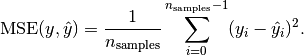
-
MAE: Mean absolute error
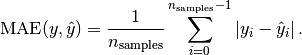
-
rsquared: coefficient of determination
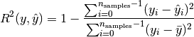
-
explained_variance
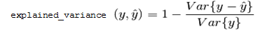
-
fscore
(1 + beta˄2) * precison * recall / (beta˄2 * precision + recall)
beta equals 1 by default
-
auc_roc: AUC of ROC using the specified number of bins, by default 100
-
auc_prc: AUC of PRC using the specified number of bins, by default 100
-
counts: Shortcut that resolves to four other metrics: TP, FP, TN, and FN
-
count: Valid only in JSON syntax, counts the number of cases labeled by one class (case-class-label) but predicted as another class (predicted-class-label):
cv_metrics='[{"count":[case-class-label, predicted-class-label]}]'
cv_fold_count- The number of folds to split the data.
Default: 5
cv_hyperparams- A JSON string that describes the combination of parameters for use in grid search of hyper parameters. The JSON string contains pairs of the hyper parameter name. The value of each hyper parameter can be specified as an array or sequence. For example:
{"param1":[value1,value2,...], "param2":{"first":first_value, "step":step_size, "count":number_of_values} }
Hyper parameter names and string values should be quoted using the JSON standard. These parameters are passed to the training function.
cv_prediction_cutoff- The cutoff threshold that is passed to the prediction stage of logistic regression, a FLOAT between 0 and 1, exclusive
Default: 0.5
Model attributes
call_string- The value of all input arguments that were specified at the time
CROSS_VALIDATE was called.
run_average- The average across all folds of all metrics specified in parameter
cv_metrics, if specified; otherwise, average accuracy.
fold_info- The number of rows in each fold:
counters- All counters for the function, including:
-
accepted_row_count: The total number of rows in the input_relation, minus the number of rejected rows.
-
rejected_row_count: The number of rows of the input_relation that were skipped because they contained an invalid value.
-
feature_count: The number of features input to the machine learning model.
run_details- Information about each run, where a run means training a single model, and then testing that model on the one held-out fold:
-
fold_id: The index of the fold held out for testing.
-
iteration_count: The number of iterations used in model training on non-held-out folds.
-
accuracy: All metrics specified in parameter cv_metrics, or accuracy if cv_metrics is not provided.
-
error_rate: All metrics specified in parameter cv_metrics, or accuracy if the parameter is omitted.
Privileges
Non-superusers:
-
SELECT privileges on the input relation
-
CREATE and USAGE privileges on the default schema where machine learning algorithms generate models. If cv_model_name is provided, the cross validation results are saved as a model in the same schema.
Specifying metrics in JSON
Parameter cv_metrics can specify metrics as an array of JSON objects, where each object specifies a metric name . For example, the following expression sets cv_metrics to two metrics specified as JSON objects, accuracy and error_rate:
cv_metrics='["accuracy", "error_rate"]'
In the next example, cv_metrics is set to two metrics, accuracy and TPR (true positive rate). Here, the TPR metric is specified as a JSON object that takes an array of two class label arguments, 2 and 3:
cv_metrics='[ "accuracy", {"TPR":[2,3] } ]'
Metrics specified as JSON objects can accept parameters. In the following example, the fscore metric specifies parameter beta, which is set to 0.5:
cv_metrics='[ {"fscore":{"beta":0.5} } ]'
Parameter support can be especially useful for certain metrics. For example, metrics auc_roc and auc_prc build a curve, and then compute the area under that curve. For ROC, the curve is formed by plotting metrics TPR against FPR; for PRC, PPV (precision) against TPR (recall). The accuracy of such curves can be increased by setting parameter num_bins to a value greater than the default value of 100. For example, the following expression computes AUC for an ROC curve built with 1000 bins:
cv_metrics='[{"auc_roc":{"num_bins":1000}}]'
Using metrics with Multi-class classifier functions
All supported metrics are defined for binary classifier functions
LOGISTIC_REG and
SVM_CLASSIFIER. For multi-class classifier functions such as
NAIVE_BAYES, these metrics can be calculated for each one-versus-the-rest binary classifier. Use arguments to request the metrics for each classifier. For example, if training data has integer class labels, you can set cv_metrics with the precision (PPV) metric as follows:
cv_metrics='[{"precision":[0,4]}]'
This setting specifies to return two columns with precision computed for two classifiers:
If you omit class label arguments, the class with index 1 is used. Instead of computing metrics for individual one-versus-the-rest classifiers, the average is computed in one of the following styles: macro, micro, or weighted (default). For example, the following cv_metrics setting returns the average weighted by class sizes:
cv_metrics='[{"precision":{"avg":"weighted"}}]'
AUC-type metrics can be similarly defined for multi-class classifiers. For example, the following cv_metrics setting computes the area under the ROC curve for each one-versus-the-rest classifier, and then returns the average weighted by class sizes.
cv_metrics='[{"auc_roc":{"avg":"weighted", "num_bins":1000}}]'
Examples
=> SELECT CROSS_VALIDATE('svm_classifier', 'mtcars', 'am', 'mpg'
      USING PARAMETERS cv_fold_count= 6,
                       cv_hyperparams='{"C":[1,5]}',
                       cv_model_name='cv_svm',
                       cv_metrics='accuracy, error_rate');
         CROSS_VALIDATE
----------------------------
 Finished

===========
run_average
===========
C  |accuracy      |error_rate
---+--------------+----------
1 | 0.75556       |  0.24444
5 | 0.78333       |  0.21667
(1 row)
3.3 - ERROR_RATE
Using an input table, returns a table that calculates the rate of incorrect classifications and displays them as FLOAT values.
Using an input table, returns a table that calculates the rate of incorrect classifications and displays them as FLOAT values. ERROR_RATE returns a table with the following dimensions:
Syntax
ERROR_RATE ( targets, predictions [ USING PARAMETERS num_classes = num-classes ] ) OVER()
Arguments
targets- An input column that contains the true values of the response variable.
predictions- An input column that contains the predicted class labels.
Arguments targets and predictions must be set to input columns of the same data type, one of the following: INTEGER, BOOLEAN, or CHAR/VARCHAR. Depending on their data type, these columns identify classes as follows:
-
INTEGER: Zero-based consecutive integers between 0 and (num-classes-1) inclusive, where num-classes is the number of classes. For example, given the following input column values— {0, 1, 2, 3, 4}—Vertica assumes five classes.
Note
If input column values are not consecutive, Vertica interpolates the missing values. Thus, given the following input values— {0, 1, 3, 5, 6,}— Vertica assumes seven classes.
-
BOOLEAN: Yes or No
-
CHAR/VARCHAR: Class names. If the input columns are of type CHAR/VARCHAR columns, you must also set parameter num_classes to the number of classes.
Note
Vertica computes the number of classes as the union of values in both input columns. For example, given the following sets of values in the targets and predictions input columns, Vertica counts four classes:
{'milk', 'soy milk', 'cream'}
{'soy milk', 'almond milk'}
Parameters
num_classesAn integer > 1, specifies the number of classes to pass to the function.
You must set this parameter if the specified input columns are of type CHAR/VARCHAR. Otherwise, the function processes this parameter according to the column data types:
-
INTEGER: By default set to 2, you must set this parameter correctly if the number of classes is any other value.
-
BOOLEAN: By default set to 2, cannot be set to any other value.
Privileges
Non-superusers: model owner, or USAGE privileges on the model
Examples
This example shows how to execute the ERROR_RATE function on an input table named mtcars. The response variables appear in the column obs, while the prediction variables appear in the column pred. Because this example is a classification problem, all response variable values and prediction variable values are either 0 or 1, indicating binary classification.
In the table returned by the function, the first column displays the class id column. The second column displays the corresponding error rate for the class id. The third column indicates how many rows were successfully used by the function and whether any rows were ignored.
=> SELECT ERROR_RATE(obs::int, pred::int USING PARAMETERS num_classes=2) OVER()
    FROM (SELECT am AS obs, PREDICT_LOGISTIC_REG (mpg, cyl, disp, drat, wt, qsec, vs, gear, carb
                USING PARAMETERS model_name='myLogisticRegModel', type='response') AS pred
             FROM mtcars) AS prediction_output;
 class |     error_rate     |                   comment
-------+--------------------+---------------------------------------------
     0 |                  0 |
     1 | 0.0769230797886848 |
       |            0.03125 | Of 32 rows, 32 were used and 0 were ignored
(3 rows)
3.4 - LIFT_TABLE
Returns a table that compares the predictive quality of a machine learning model.
Returns a table that compares the predictive quality of a machine learning model. This function is also known as a lift chart.
Syntax
LIFT_TABLE ( targets, probabilities
        [ USING PARAMETERS [num_bins = num-bins] [, main_class = class-name ] ] )
OVER()
Arguments
targets- An input column that contains the true values of the response variable, one of the following data types: INTEGER, BOOLEAN, or CHAR/VARCHAR. Depending on the column data type, the function processes column data as follows:
-
INTEGER: Uses the input column as containing the true value of the response variable.
-
BOOLEAN: Resolves Yes to 1, 0 to No.
-
CHAR/VARCHAR: Resolves the value specified by parameter main_class to 1, all other values to 0.
Note
If the input column is of data type INTEGER or BOOLEAN, the function ignores parameter main_class.
probabilities- A FLOAT input column that contains the predicted probability of response being the main class, set to 1 if
targets is of type INTEGER.
Parameters
num_binsAn integer value that determines the number of decision boundaries. Decision boundaries are set at equally spaced intervals between 0 and 1, inclusive. The function computes the table at each num-bin + 1 point.
Default: 100
main_classUsed only if targets is of type CHAR/VARCHAR, specifies the class to associate with the probabilities argument.
Examples
Execute LIFT_TABLE on an input table mtcars.
=> SELECT LIFT_TABLE(obs::int, prob::float USING PARAMETERS num_bins=2) OVER()
    FROM (SELECT am AS obs, PREDICT_LOGISTIC_REG(mpg, cyl, disp, drat, wt, qsec, vs, gear, carb
                                                    USING PARAMETERS model_name='myLogisticRegModel',
                                                    type='probability') AS prob
             FROM mtcars) AS prediction_output;
 decision_boundary | positive_prediction_ratio |       lift       |                   comment
-------------------+---------------------------+------------------+---------------------------------------------
                 1 |                         0 |              NaN |
               0.5 |                   0.40625 | 2.46153846153846 |
                 0 |                         1 |                1 | Of 32 rows, 32 were used and 0 were ignored
(3 rows)
The first column, decision_boundary, indicates the cut-off point for whether to classify a response as 0 or 1. For instance, for each row, if prob is greater than or equal to decision_boundary, the response is classified as 1. If prob is less than decision_boundary, the response is classified as 0.
The second column, positive_prediction_ratio, shows the percentage of samples in class 1 that the function classified correctly using the corresponding decision_boundary value.
For the third column, lift, the function divides the positive_prediction_ratio by the percentage of rows correctly or incorrectly classified as class 1.
3.5 - MSE
Returns a table that displays the mean squared error of the prediction and response columns in a machine learning model.
Returns a table that displays the mean squared error of the prediction and response columns in a machine learning model.
Syntax
MSE ( targets, predictions ) OVER()
Arguments
targets- The model response variable, of type FLOAT.
predictions- A FLOAT input column that contains predicted values for the response variable.
Examples
Execute the MSE function on input table faithful_testing. The response variables appear in the column obs, while the prediction variables appear in the column prediction.
=> SELECT MSE(obs, prediction) OVER()
   FROM (SELECT eruptions AS obs,
                PREDICT_LINEAR_REG (waiting USING PARAMETERS model_name='myLinearRegModel') AS prediction
         FROM faithful_testing) AS prediction_output;
        mse        |                   Comments
-------------------+-----------------------------------------------
 0.252925741352641 | Of 110 rows, 110 were used and 0 were ignored
(1 row)
3.6 - PRC
Returns a table that displays the points on a receiver precision recall (PR) curve.
Returns a table that displays the points on a receiver precision recall (PR) curve.
Syntax
PRC ( targets, probabilities
       [ USING PARAMETERS
             [num_bins = num-bins]
             [, f1_score = return-score ]
             [, main_class = class-name ] )
OVER()
Arguments
targets- An input column that contains the true values of the response variable, one of the following data types: INTEGER, BOOLEAN, or CHAR/VARCHAR. Depending on the column data type, the function processes column data as follows:
-
INTEGER: Uses the input column as containing the true value of the response variable.
-
BOOLEAN: Resolves Yes to 1, 0 to No.
-
CHAR/VARCHAR: Resolves the value specified by parameter main_class to 1, all other values to 0.
Note
If the input column is of data type INTEGER or BOOLEAN, the function ignores parameter main_class.
probabilities- A FLOAT input column that contains the predicted probability of response being the main class, set to 1 if
targets is of type INTEGER.
Parameters
num_binsAn integer value that determines the number of decision boundaries. Decision boundaries are set at equally spaced intervals between 0 and 1, inclusive. The function computes the table at each num-bin + 1 point.
Default: 100
f1_score- A Boolean that specifies whether to return a column that contains the f1 score—the harmonic average of the precision and recall measures, where an F1 score reaches its best value at 1 (perfect precision and recall) and worst at 0.
Default: false
main_classUsed only if targets is of type CHAR/VARCHAR, specifies the class to associate with the probabilities argument.
Examples
Execute the PRC function on an input table named mtcars. The response variables appear in the column obs, while the prediction variables appear in column pred.
=> SELECT PRC(obs::int, prob::float USING PARAMETERS num_bins=2, f1_score=true) OVER()
    FROM (SELECT am AS obs,
                    PREDICT_LOGISTIC_REG (mpg, cyl, disp, drat, wt, qsec, vs, gear, carb
                          USING PARAMETERS model_name='myLogisticRegModel',
                                           type='probability') AS prob
             FROM mtcars) AS prediction_output;
decision_boundary | recall | precision |     f1_score      |     comment
------------------+--------+-----------+-------------------+--------------------------------------------
0                 |      1 |   0.40625 | 0.577777777777778 |
0.5               |      1 |         1 |                 1 | Of 32 rows, 32 were used and 0 were ignored
(2 rows)
The first column, decision_boundary, indicates the cut-off point for whether to classify a response as 0 or 1. For example, in each row, if the probability is equal to or greater than decision_boundary, the response is classified as 1. If the probability is less than decision_boundary, the response is classified as 0.
3.7 - READ_TREE
Reads the contents of trees within the random forest or XGBoost model.
Reads the contents of trees within the random forest or XGBoost model.
Syntax
READ_TREE ( USING PARAMETERS model_name = 'model-name' [, tree_id = tree-id] [, format = 'format'] )
Parameters
model_name- Identifies the model that is stored as a result of training, where
model-name conforms to conventions described in Identifiers. It must also be unique among all names of sequences, tables, projections, views, and models within the same schema.
tree_id- The tree identifier, an integer between 0 and
n-1, where n is the number of trees in the random forest or XGBoost model. If you omit this parameter, all trees are returned.
format- Output format of the returned tree, one of the following:
Privileges
Non-superusers: USAGE privileges on the model
Examples
Get tabular output from READ_TREE for a random forest model:
=> SELECT READ_TREE ( USING PARAMETERS model_name='myRFModel', tree_id=1 ,
format= 'tabular') LIMIT 2;
-[ RECORD 1 ]-------------+-------------------
tree_id                   | 1
node_id                   | 1
node_depth                | 0
is_leaf                   | f
is_categorical_split      | f
split_predictor           | petal_length
split_value               | 1.921875
weighted_information_gain | 0.111242236024845
left_child_id             | 2
right_child_id            | 3
prediction                |
probability/variance      |

-[ RECORD 2 ]-------------+-------------------
tree_id                   | 1
node_id                   | 2
node_depth                | 1
is_leaf                   | t
is_categorical_split      |
split_predictor           |
split_value               |
weighted_information_gain |
left_child_id             |
right_child_id            |
prediction                | setosa
probability/variance      | 1
Get graphviz-formatted output from READ_TREE:
=> SELECT READ_TREE ( USING PARAMETERS model_name='myRFModel', tree_id=1 ,
format= 'graphviz')LIMIT 1;

-[ RECORD 1 ]+-------------------------------------------------------------------
---------------------------------------------------------------------------------
tree_id      | 1
tree_digraph | digraph Tree{
1 [label="petal_length < 1.921875 ?", color="blue"];
1 -> 2 [label="yes", color="black"];
1 -> 3 [label="no", color="black"];
2 [label="prediction: setosa, probability: 1", color="red"];
3 [label="petal_length < 4.871875 ?", color="blue"];
3 -> 6 [label="yes", color="black"];
3 -> 7 [label="no", color="black"];
6 [label="prediction: versicolor, probability: 1", color="red"];
7 [label="prediction: virginica, probability: 1", color="red"];
}
This renders as follows:
See also
3.8 - RF_PREDICTOR_IMPORTANCE
Measures the importance of the predictors in a random forest model using the Mean Decrease Impurity (MDI) approach.
Measures the importance of the predictors in a random forest model using the Mean Decrease Impurity (MDI) approach. The importance vector is normalized to sum to 1.
Syntax
RF_PREDICTOR_IMPORTANCE ( USING PARAMETERS model_name = 'model-name' [, tree_id = tree-id] )
Parameters
model_name- Identifies the model that is stored as a result of the training, where
model-name must be of type rf_classifier or rf_regressor.
tree_id- Identifies the tree to process, an integer between 0 and
n-1, where n is the number of trees in the forest. If you omit this parameter, the function uses all trees to measure importance values.
Privileges
Non-superusers: USAGE privileges on the model
Examples
This example shows how you can use the RF_PREDICTOR_IMPORTANCE function.
=> SELECT RF_PREDICTOR_IMPORTANCE ( USING PARAMETERS model_name = 'myRFModel');
 predictor_index | predictor_name | importance_value
-----------------+----------------+--------------------
               0 | sepal.length   | 0.106763318092655
               1 | sepal.width    | 0.0279536658041994
               2 | petal.length   | 0.499198722346586
               3 | petal.width    | 0.366084293756561
(4 rows)
See also
3.9 - ROC
Returns a table that displays the points on a receiver operating characteristic curve.
Returns a table that displays the points on a receiver operating characteristic curve. The ROC function tells you the accuracy of a classification model as you raise the discrimination threshold for the model.
Syntax
ROC ( targets, probabilities
        [ USING PARAMETERS
              [num_bins = num-bins]
              [, AUC = output]
              [, main_class = class-name ] ) ] )
OVER()
Arguments
targets- An input column that contains the true values of the response variable, one of the following data types: INTEGER, BOOLEAN, or CHAR/VARCHAR. Depending on the column data type, the function processes column data as follows:
-
INTEGER: Uses the input column as containing the true value of the response variable.
-
BOOLEAN: Resolves Yes to 1, 0 to No.
-
CHAR/VARCHAR: Resolves the value specified by parameter main_class to 1, all other values to 0.
Note
If the input column is of data type INTEGER or BOOLEAN, the function ignores parameter main_class.
probabilities- A FLOAT input column that contains the predicted probability of response being the main class, set to 1 if
targets is of type INTEGER.
Parameters
num_binsAn integer value that determines the number of decision boundaries. Decision boundaries are set at equally spaced intervals between 0 and 1, inclusive. The function computes the table at each num-bin + 1 point.
Default: 100
Greater values result in more precise approximations of the AUC.
AUC- A Boolean value that specifies whether to output the area under the curve (AUC) value.
Default: True
main_classUsed only if targets is of type CHAR/VARCHAR, specifies the class to associate with the probabilities argument.
Examples
Execute ROC on input table mtcars. Observed class labels are in column obs, predicted class labels are in column prob:
=> SELECT ROC(obs::int, prob::float USING PARAMETERS num_bins=5, AUC = True) OVER()
    FROM (SELECT am AS obs,
          PREDICT_LOGISTIC_REG (mpg, cyl, disp, drat, wt, qsec, vs, gear, carb
               USING PARAMETERS
                  model_name='myLogisticRegModel', type='probability') AS prob
   FROM mtcars) AS prediction_output;
 decision_boundary | false_positive_rate | true_positive_rate | AUC |comment
-------------------+---------------------+--------------------+-----+-----------------------------------
0                  |                   1 |                  1 |     |
0.5                |                   0 |                  1 |     |
1                  |                   0 |                  0 |   1 | Of 32 rows,32 were used and 0 were ignoreded
(3 rows)
The function returns a table with the following results:
-
decision_boundary indicates the cut-off point for whether to classify a response as 0 or 1. In each row, if prob is equal to or greater than decision_boundary, the response is classified as 1. If prob is less than decision_boundary, the response is classified as 0.
-
false_positive_rate shows the percentage of false positives (when 0 is classified as 1) in the corresponding decision_boundary.
-
true_positive_rate shows the percentage of rows that were classified as 1 and also belong to class 1.
3.10 - RSQUARED
Returns a table with the R-squared value of the predictions in a regression model.
Returns a table with the R-squared value of the predictions in a regression model.
Syntax
RSQUARED ( targets, predictions ) OVER()
Important
The OVER() clause must be empty.
Arguments
targets- A FLOAT response variable for the model.
predictions- A FLOAT input column that contains the predicted values for the response variable.
Examples
This example shows how to execute the RSQUARED function on an input table named faithful_testing. The observed values of the response variable appear in the column, obs, while the predicted values of the response variable appear in the column, pred.
=> SELECT RSQUARED(obs, prediction) OVER()
     FROM (SELECT eruptions AS obs,
                  PREDICT_LINEAR_REG (waiting
                                       USING PARAMETERS model_name='myLinearRegModel') AS prediction
           FROM faithful_testing) AS prediction_output;
        rsq        |                    comment
-------------------+-----------------------------------------------
 0.801392981147911 | Of 110 rows, 110 were used and 0 were ignored
(1 row)
3.11 - XGB_PREDICTOR_IMPORTANCE
Measures the importance of the predictors in an XGBoost model.
Measures the importance of the predictors in an XGBoost model. The function outputs three measures of importance for each predictor:
-
frequency: relative number of times the model uses a predictor to split the data.
-
total_gain: relative contribution of a predictor to the model based on the total information gain across a predictor's splits. A higher value means more predictive importance.
-
avg_gain: relative contribution of a predictor to the model based on the average information gain across a predictor's splits.
The sum of each importance measure is normalized to one across all predictors.
Syntax
XGB_PREDICTOR_IMPORTANCE ( USING PARAMETERS param=value[,...] )
Parameters
model_name- Name of the model, which must be of type
xgb_classifier or xgb_regressor.
tree_id- Integer in the range [0,
n-1], where n is the number of trees in model_name, that specifies the tree to process. If you omit this parameter, the function uses all trees in the model to measure predictor importance values.
Privileges
Non-superusers: USAGE privileges on the model
Examples
The following example measures the importance of the predictors in the model 'xgb_iris', an XGBoost classifier model, across all trees:
=> SELECT XGB_PREDICTOR_IMPORTANCE( USING PARAMETERS model_name = 'xgb_iris' );
 predictor_index | predictor_name |     frequency     |     total_gain     |      avg_gain
-----------------+----------------+-------------------+--------------------+--------------------
               0 | sepal_length   |  0.15384615957737 |    0.0183021749937 | 0.0370849960701401
               1 | sepal_width    | 0.215384617447853 | 0.0154729501420881 | 0.0223944615251752
               2 | petal_length   | 0.369230777025223 |  0.607349886817728 |  0.512770753876444
               3 | petal_width    | 0.261538475751877 |  0.358874988046484 |  0.427749788528241
(4 rows)
To sort the predictors by importance values, you can use a nested query with an ORDER BY clause. The following sorts the model predictors by descending avg_gain:
=> SELECT * FROM (SELECT XGB_PREDICTOR_IMPORTANCE( USING PARAMETERS model_name = 'xgb_iris' )) AS importances ORDER BY avg_gain DESC;
 predictor_index | predictor_name |     frequency     |     total_gain     |      avg_gain
-----------------+----------------+-------------------+--------------------+--------------------
               2 | petal_length   | 0.369230777025223 |  0.607349886817728 |  0.512770753876444
               3 | petal_width    | 0.261538475751877 |  0.358874988046484 |  0.427749788528241
               0 | sepal_length   |  0.15384615957737 |    0.0183021749937 | 0.0370849960701401
               1 | sepal_width    | 0.215384617447853 | 0.0154729501420881 | 0.0223944615251752
(4 rows)
See also
4 - Model management
Vertica provides several functions for managing models.
Vertica provides several functions for managing models.
4.1 - CHANGE_MODEL_STATUS
Changes the status of a registered model.
Changes the status of a registered model. Only dbadmin and users with the MLSUPERVISOR role can call this function.
The following diagram depicts the valid status transitions:
This is a meta-function. You must call meta-functions in a top-level SELECT statement.
Behavior type
Stable
Syntax
CHANGE_MODEL_STATUS( 'registered_name', registered_version, 'new_status' )
Arguments
registered_name- Identifies the abstract name to which the model is registered. This
registered_name can represent a group of models for a higher-level application, where each model in the group has a unique version number.
registered_version- Unique version number of the model under the specified
registered_name.
If there is no registered model with the given registered_name and registered_version, the function errors.
new_status- New status of the registered model. Must be one of the following strings and adhere to the valid status transitions depicted in the above diagram:
-
under_review: Status assigned to newly registered models.
-
staging: Model is targeted for A/B testing against the model currently in production.
-
production: Model is in production for its specified application. Only one model can be in production for a given registered_name at one time.
-
archived: Status of models that were previously in production. Archived models can be returned to production at any time.
-
declined: Model is no longer in consideration for production.
-
unregistered: Model is removed from the versioning environment. The model does not appear in the REGISTERED_MODELS system table.
If you change the status of a model to 'production' and there is already a model in production under the given registered_name, the status of the model in production is set to 'archived' and the status of the new model is set to 'production'.
Privileges
One of the following:
Examples
In the following example, the linear_reg_spark1 model, which is uniquely identified by the registered_name 'linear_reg_app' and the registered_version of two, is set to 'production' status:
=> SELECT * FROM REGISTERED_MODELS;
  registered_name | registered_version |    status    |        registered_time        |      model_id     | schema_name |    model_name     |      model_type       |    category
------------------+--------------------+--------------+-------------------------------+-------------------+-------------+-------------------+-----------------------+----------------
 linear_reg_app   |                  2 | STAGING      | 2023-01-29 05:49:00.082166-04 | 45035996273714020 | public      | linear_reg_spark1 | PMML_REGRESSION_MODEL | PMML
 linear_reg_app   |                  1 | PRODUCTION   | 2023-01-24 09:19:04.553102-05 | 45035996273850350 | public      | native_linear_reg | LINEAR_REGRESSION     | VERTICA_MODELS
 logistic_reg_app |                  1 | DECLINED     | 2023-01-11 02:47:25.990626-02 | 45035996273853740 | public      | log_reg_bfgs      | LOGISTIC_REGRESSION   | VERTICA_MODELS
(3 rows)

=> SELECT CHANGE_MODEL_STATUS('linear_reg_app', 2, 'production');
                          CHANGE_MODEL_STATUS
-----------------------------------------------------------------------------
The status of model [linear_reg_app] - version [2] is changed to [production]
(1 row)
You can query the REGISTERED_MODELS system table to confirm that the linear_reg_spark1 model is now in 'production' and the native_linear_reg model, which was currently in 'production', is moved to 'archived':
=> SELECT * FROM REGISTERED_MODELS;
  registered_name | registered_version |    status    |        registered_time        |      model_id     | schema_name |    model_name     |      model_type       |    category
------------------+--------------------+--------------+-------------------------------+-------------------+-------------+-------------------+-----------------------+----------------
 linear_reg_app   |                  2 | PRODUCTION   | 2023-01-29 05:49:00.082166-04 | 45035996273714020 | public      | linear_reg_spark1 | PMML_REGRESSION_MODEL | PMML
 linear_reg_app   |                  1 | ARCHIVED     | 2023-01-24 09:19:04.553102-05 | 45035996273850350 | public      | native_linear_reg | LINEAR_REGRESSION     | VERTICA_MODELS
 logistic_reg_app |                  1 | DECLINED     | 2023-01-11 02:47:25.990626-02 | 45035996273853740 | public      | log_reg_bfgs      | LOGISTIC_REGRESSION   | VERTICA_MODELS
(2 rows)
If you change a model's status to 'unregistered', the model is removed from the model versioning environment and no longer appears in the REGISTERED_MODELS system table:
=> SELECT CHANGE_MODEL_STATUS('logistic_reg_app', 1, 'unregistered');
                            CHANGE_MODEL_STATUS
----------------------------------------------------------------------------------
The status of model [logistic_reg_app] - version [1] is changed to [unregistered]
(1 row)

=> SELECT * FROM REGISTERED_MODELS;
  registered_name | registered_version |    status    |        registered_time        |      model_id     | schema_name |    model_name     |      model_type       |    category
------------------+--------------------+--------------+-------------------------------+-------------------+-------------+-------------------+-----------------------+----------------
 linear_reg_app   |                  2 | STAGING      | 2023-01-29 05:49:00.082166-04 | 45035996273714020 | public      | linear_reg_spark1 | PMML_REGRESSION_MODEL | PMML
 linear_reg_app   |                  1 | PRODUCTION   | 2023-01-24 09:19:04.553102-05 | 45035996273850350 | public      | native_linear_reg | LINEAR_REGRESSION     | VERTICA_MODELS
(2 rows)
See also
4.2 - EXPORT_MODELS
Exports machine learning models.
Exports machine learning models. Vertica supports three model formats:
This is a meta-function. You must call meta-functions in a top-level SELECT statement.
Behavior type
Volatile
Syntax
EXPORT_MODELS ( 'output-dir', 'export-target' [ USING PARAMETERS category = 'model-category' ] )
Arguments
output-dir- Absolute path of an output directory to store the exported models, either an absolute path on the initiator node file system or a URI for a supported file system or object store.
export-target- Models to export:
[schema.]{model-name | * }
schema specifies the schema from which models are exported. If omitted, EXPORT_MODELS uses the default schema. Supply * (asterisk) to batch export all models from the schema.
If a model in a batch fails to export, the function issues a warning and then continues to export any remaining models in the batch. Details about any failed model exports are available in the log file generated at the output-dir location.
Parameters
category- The category of models to export, one of the following:
-
VERTICA_MODELS
-
PMML
-
TENSORFLOW
EXPORT_MODELS exports models of the specified category according to the scope of the export operation—that is, whether it applies to a single model, or to all models within a schema. See Export Scope and Category Processing below.
Exported Files below describes the files that EXPORT_MODELS exports for each category.
If you omit this parameter, EXPORT_MODELS exports the model, or models in the specified schema, according to their model type.
Privileges
Superuser or MLSUPERVISOR
Export scope and category processing
EXPORT_MODELS executes according to the following parameter settings:
-
Scope of the export operation: single model, or all models within a given schema
-
Category specified or omitted
The following table shows how these two parameters control the export process:
|
Export scope |
If category specified... |
If category omitted... |
|
Single model |
Convert the model to the specified category, provided the model and category are compatible; otherwise, return with a mismatch error. |
Export the model according to model type. |
|
All models in schema |
Export only models that are compatible with the specified category and issue mismatch warnings on all other models in the schema. |
Export all models in the schema according to model type. |
Exported files
EXPORT_MODELS exports the following files for each model category:
VERTICA_MODELS
-
Multiple binary files (exact number dependent on model type)
-
metadata.json: Metadata file with model information, including model name, category, type, and Vertica version on export.
-
crc.json: Used on import to validate other files of this model.
PMML
-
XML file with the same name as the model and complying with PMML standard.
-
metadata.json: Metadata file with model information, including model name, category, type, and Vertica version on export.
-
crc.json: Used on import to validate other files of this model.
TENSORFLOW
-
model-name.pb: Contains the TensorFlow model, saved in 'frozen graph' format.
-
metadata.json: Metadata file with model information, including model name, category, type, and Vertica version on export.
-
tf_model_desc.json: Summary model description.
-
model.json: Verbose model description.
-
crc.json: Used on import to validate other files of this model.
Categories and compatible models
If EXPORT_MODELS specifies a single model and also sets the category parameter, the function succeeds if the model type and category are compatible; otherwise, it returns with an error. The following model types are compatible with the listed categories:
PMMLPMMLTensorFlowTENSORFLOWVERTICA_MODELSPMML
VERTICA_MODELS
If EXPORT_MODELS specifies to export all models from a schema and sets a category, it issues a warning message on each model that is incompatible with that category. The function then continues to process remaining models in that schema.
EXPORT_MODELS logs all errors and warnings in output-dir/export_log.json.
Examples
Export models without changing their category
Export model myschema.mykmeansmodel without changing its category:
=> SELECT EXPORT_MODELS ('/home/dbadmin', 'myschema.mykmeansmodel');
EXPORT_MODELS
----------------
Success
(1 row)
Export all models in schema myschema without changing their categories:
=> SELECT EXPORT_MODELS ('/home/dbadmin', 'myschema.*');
EXPORT_MODELS
----------------
Success
(1 row)
Export all the models in schema models to an S3 bucket without changing the model categories:
SELECT export_models('s3://vertica/ml_models', 'models.*');
EXPORT_MODELS
---------------
Success
(1 row)
Export models that are compatible with the specified category
Note
When you import a model of category VERTICA_MODELS trained in a different version of Vertica, Vertica automatically upgrades the model version to match that of the database. If this fails, you must run UPGRADE_MODEL.
If both methods fail, the model cannot be used for in-database scoring and cannot be exported as a PMML model.
The category is set to PMML. Models of type PMML and VERTICA_MODELS are compatible with the PMML category, so the export operation succeeds if my_keans is of either type:
=> SELECT EXPORT_MODELS ('/tmp/', 'my_kmeans' USING PARAMETERS category='PMML');
The category is set to VERTICA_MODELS. Only models of type VERTICA_MODELS are compatible with the VERTICA_MODELS category, so the export operation succeeds only if my_keans is of that type:
=> SELECT EXPORT_MODELS ('/tmp/', 'public.my_kmeans' USING PARAMETERS category='VERTICA_MODELS');
The category is set to TENSORFLOW. Only models of type TensorFlow are compatible with the TENSORFLOW category, so the model tf_mnist_keras must be of type TensorFlow:
=> SELECT EXPORT_MODELS ('/tmp/', 'tf_mnist_keras', USING PARAMETERS category='TENSORFLOW');
export_models
---------------
Success
(1 row)
After exporting the TensorFlow model tf_mnist_keras, list the exported files:
$ ls tf_mnist_keras/
crc.json  metadata.json  mnist_keras.pb  model.json  tf_model_desc.json
See also
IMPORT_MODELS
4.3 - GET_MODEL_ATTRIBUTE
Extracts either a specific attribute from a model or all attributes from a model.
Extracts either a specific attribute from a model or all attributes from a model. Use this function to view a list of attributes and row counts or view detailed information about a single attribute. The output of GET_MODEL_ATTRIBUTE is a table format where users can select particular columns or rows.
Syntax
GET_MODEL_ATTRIBUTE ( USING PARAMETERS model_name = 'model-name' [, attr_name = 'attribute' ] )
Parameters
model_nameName of the model (case-insensitive).
attr_name- Name of the model attribute to extract. If omitted, the function shows all available attributes. Attribute names are case-sensitive.
Privileges
Non-superusers: model owner, or USAGE privileges on the model
Examples
This example returns a summary of all model attributes.
=> SELECT GET_MODEL_ATTRIBUTE ( USING PARAMETERS model_name='myLinearRegModel');
attr_name          |                attr_fields                        | #_of_rows
-------------------+---------------------------------------------------+-----------
details            | predictor, coefficient, std_err, t_value, p_value |         2
regularization     | type, lambda                                      |         1
iteration_count    | iteration_count                                   |         1
rejected_row_count | rejected_row_count                                |         1
accepted_row_count | accepted_row_count                                |         1
call_string        | call_string                                       |         1
(6 rows)
This example extracts the details attribute from the myLinearRegModel model.
=> SELECT GET_MODEL_ATTRIBUTE ( USING PARAMETERS model_name='myLinearRegModel', attr_name='details');
coeffNames |       coeff        |       stdErr        |      zValue       |        pValue
-----------+--------------------+---------------------+-------------------+-----------------------
Intercept  |  -1.87401598641074 |   0.160143331525544 | -11.7021169008952 |   7.3592939615234e-26
waiting    | 0.0756279479518627 | 0.00221854185633525 |  34.0890336307608 | 8.13028381124448e-100
(2 rows)
4.4 - GET_MODEL_SUMMARY
Returns summary information of a model.
Returns summary information of a model.
Syntax
GET_MODEL_SUMMARY ( USING PARAMETERS model_name = 'model-name' )
Parameters
- model_name
Name of the model (case-insensitive).
Privileges
Non-superusers: model owner, or USAGE privileges on the model
Examples
This example shows how you can view the summary of a linear regression model.
=> SELECT GET_MODEL_SUMMARY( USING PARAMETERS model_name='myLinearRegModel');

--------------------------------------------------------------------------------
=======
details
=======
predictor|coefficient|std_err |t_value |p_value
---------+-----------+--------+--------+--------
Intercept| -2.06795  | 0.21063|-9.81782| 0.00000
waiting  |  0.07876  | 0.00292|26.96925| 0.00000

==============
regularization
==============
type| lambda
----+--------
none| 1.00000

===========
call_string
===========
linear_reg('public.linear_reg_faithful', 'faithful_training', '"eruptions"', 'waiting'
USING PARAMETERS optimizer='bfgs', epsilon=1e-06, max_iterations=100,
regularization='none', lambda=1)

===============
Additional Info
===============
Name              |Value
------------------+-----
iteration_count   |  3
rejected_row_count|  0
accepted_row_count| 162
(1 row)
4.5 - IMPORT_MODELS
Imports models into Vertica, either Vertica models that were exported with EXPORT_MODELS, or models in Predictive Model Markup Language (PMML) or TensorFlow format.
Imports models into Vertica, either Vertica models that were exported with EXPORT_MODELS, or models in Predictive Model Markup Language (PMML) or TensorFlow format. You can use this function to move models between Vertica clusters, or to import PMML and TensorFlow models trained elsewhere.
Other Vertica model management operations such as GET_MODEL_SUMMARY and GET_MODEL_ATTRIBUTE support imported models.
Caution
Changing the exported model files causes the import functionality to fail on attempted re-import.
This is a meta-function. You must call meta-functions in a top-level SELECT statement.
Behavior type
Volatile
Syntax
IMPORT_MODELS ( 'source'
           [ USING PARAMETERS [ new_schema = 'schema-name' ] [, category = 'model-category' ] ] )
Arguments
source- Path from which to import models, either an absolute path on the initiator node file system or a URI for a supported file system or object store. The path format depends on whether you are importing a single model or a batch of models:
-
To import a single model, provide the path to the model's directory:
path/model-directory
-
To import a batch of models, provide the path to a parent directory that contains the model directories for each model in the batch:
parent-dir-path/*
If a model in a batch fails to import, the function issues a warning and then continues to import any remaining models in the batch. Details about any failed model import are available in the log file generated at the source location.
Parameters
new_schema- An existing schema where the machine learning models are imported. If omitted, models are imported to the default schema.
IMPORT_MODELS extracts the name of the imported model from its metadata.json file, if it exists. Otherwise, the function uses the name of the model directory.
category- Specifies the category of the model to import, one of the following:
-
VERTICA_MODELS
-
PMML
-
TENSORFLOW
This parameter is required if the model directory has no metadata.json file. IMPORT_MODELS returns with an error if one of the following cases is true:
Note
If the category is TENSORFLOW, IMPORT_MODELS only imports the following files from the model directory:
Privileges
Superuser or MLSUPERVISOR
Requirements and restrictions
The following requirements and restrictions apply:
-
If you export a model, then import it again, the export and import model directory names must match. If naming conflicts occur, import the model to a different schema by using the new_schema parameter, and then rename the model.
-
The machine learning configuration parameter MaxModelSizeKB sets the maximum size of a model that can be imported into Vertica.
-
Some PMML features and attributes are not currently supported. See PMML features and attributes for details.
-
If you import a PMML model with both metadata.json and crc.json files, the CRC file must contain the metadata file's CRC value. Otherwise, the import operation returns with an error.
Examples
If no model category is specified, IMPORT_MODELS uses the model's metadata.json file to determine its category.
Import a single model mykmeansmodel into the newschema schema:
=> SELECT IMPORT_MODELS ('/home/dbadmin/myschema/mykmeansmodel' USING PARAMETERS new_schema='newschema')
IMPORT_MODELS
----------------
Success
(1 row)
Import all models in the myschema directory into the newschema schema:
=> SELECT IMPORT_MODELS ('/home/dbadmin/myschema/*' USING PARAMETERS new_schema='newschema')
IMPORT_MODELS
----------------
Success
(1 row)
Import the model tf_mnsit_estimator from an S3 bucket into the ml_models schema:
=> SELECT IMPORT_MODELS ('s3://ml-models/tensorflow/mnist' USING PARAMETERS new_schema='ml_models')
IMPORT MODELS
---------------
Success
(1 row)
When you set the category parameter, the specified category must match the model type of the imported models; otherwise, the function returns an error.
Import kmeans_pmml as a PMML model:
SELECT IMPORT_MODELS ('/root/user/kmeans_pmml' USING PARAMETERS category='PMML')
 import_models
---------------
 Success
(1 row)
Attempt to import kmeans_pmml, a PMML model, as a TENSORFLOW model:
SELECT IMPORT_MODELS ('/root/user/kmeans_pmml' USING PARAMETERS category='TENSORFLOW')
                import_models
-------------------------------------------------
Has failure. Please check import_log.json file
(1 row)
Import tf_mnist_estimator as a TensorFlow model:
=> SELECT IMPORT_MODELS ( '/path/tf_models/tf_mnist_estimator' USING PARAMETERS category='TENSORFLOW');
 import_models
---------------
 Success
(1 row)
Import all TensorFlow models from the specified directory:
=> SELECT IMPORT_MODELS ( '/path/tf_models/*' USING PARAMETERS category='TENSORFLOW');
 import_models
---------------
 Success
(1 row)
See also
EXPORT_MODELS
4.6 - REGISTER_MODEL
Registers a trained model and adds it to Model Versioning environment with a status of 'under_review'.
Registers a trained model and adds it to Model versioning environment with a status of 'under_review'. The model must be registered by the owner of the model, dbadmin, or MLSUPERVISOR.
After a model is registered, the model owner is automatically changed to Superuser and the previous owner is given USAGE privileges. Users with the MLSUPERVISOR role or dbamin can call the CHANGE_MODEL_STATUS function to alter the status of registered models.
This is a meta-function. You must call meta-functions in a top-level SELECT statement.
Behavior type
Stable
Syntax
REGISTER_MODEL( 'model_name', 'registered_name' )
Arguments
model_name- Identifies the model to register. If the model has already been registered, the function throws an error.
registered_name- Identifies an abstract name to which the model is registered. This
registered_name can represent a group of models for a higher-level application, where each model in the group has a unique version number.
If a model is the first to be registered to a given registered_name, the model is assigned a registered_version of one. Otherwise, newly registered models are assigned an incremented registered_version of n + 1, where n is the number of models already registered to the given registered_name. Each registered model can be uniquely identified by the combination of registered_name and registered_version.
Privileges
Non-superusers: model owner
Examples
In the following example, the model log_reg_bfgs is registered to the logistic_reg_app application:
=> SELECT REGISTER_MODEL('log_reg_bfgs', 'logistic_reg_app');
                          REGISTER_MODEL
----------------------------------------------------------------------
Model [log_reg_bfgs] is registered as [logistic_reg_app], version [1]
(1 row)
You can query the REGISTERED_MODELS system table to view details about the newly registered model:
=> SELECT * FROM REGISTERED_MODELS;
  registered_name | registered_version |    status    |        registered_time        |      model_id     | schema_name |    model_name     |      model_type       |    category
------------------+--------------------+--------------+-------------------------------+-------------------+-------------+-------------------+-----------------------+----------------
 logistic_reg_app |                  1 | UNDER_REVIEW | 2023-01-22 09:49:25.990626-02 | 45035996273853740 | public      | log_reg_bfgs      | LOGISTIC_REGRESSION   | VERTICA_MODELS
(1 row)
See also
4.7 - UPGRADE_MODEL
Upgrades a model from a previous Vertica version.
Upgrades a model from a previous Vertica version. Vertica automatically runs this function during a database upgrade and if you run the IMPORT_MODELS function. Manually call this function to upgrade models after a backup or restore.
If UPGRADE_MODEL fails to upgrade the model and the model is of category VERTICA_MODELS, it cannot be used for in-database scoring and cannot be exported as a PMML model.
This is a meta-function. You must call meta-functions in a top-level SELECT statement.
Behavior type
Volatile
Syntax
UPGRADE_MODEL ( [ USING PARAMETERS [model_name = 'model-name'] ] )
Parameters
model_name- Name of the model to upgrade. If you omit this parameter, Vertica upgrades all models on which you have privileges.
Privileges
Non-superuser: Upgrades only models that the user owns.
Examples
Upgrade model myLogisticRegModel:
=> SELECT UPGRADE_MODEL( USING PARAMETERS model_name = 'myLogisticRegModel');
        UPGRADE_MODEL
----------------------------
 1 model(s) upgrade

(1 row)
Upgrade all models that the user owns:
=> SELECT UPGRADE_MODEL();
        UPGRADE_MODEL
----------------------------
 20 model(s) upgrade

(1 row)
5 - Transformation functions
The machine learning API includes a set of UDx functions that transform the columns of each input row to one or more corresponding output columns.
The machine learning API includes a set of UDx functions that transform the columns of each input row to one or more corresponding output columns. These transformations follow rules that are defined in models that were created earlier. For example,
APPLY_SVD uses an SVD model to transform input data.
Unless otherwise indicated, these functions require the following privileges for non-superusers:
In general, given an invalid input row, the return value for these functions is NULL.
5.1 - APPLY_BISECTING_KMEANS
Applies a trained bisecting k-means model to an input relation, and assigns each new data point to the closest matching cluster in the trained model.
Applies a trained bisecting k-means model to an input relation, and assigns each new data point to the closest matching cluster in the trained model.
Note
If the input relation is defined in Hive, use
SYNC_WITH_HCATALOG_SCHEMA to sync the
hcatalog schema, and then run the machine learning function.
Syntax
SELECT APPLY_BISECTING_KMEANS( 'input-columns'
        USING PARAMETERS model_name = 'model-name'
            [, num_clusters = 'num-clusters']
            [, match_by_pos = match-by-position] ] )
Arguments
input-columns- Comma-separated list of columns to use from the input relation, or asterisk (*) to select all columns. Input columns must be of data type numeric.
Parameters
model_nameName of the model (case-insensitive).
num_clusters- Integer between 1 and
k inclusive, where k is the number of centers in the model, specifies the number of clusters to use for prediction.
Default: Value that the model specifies for k
match_by_posBoolean value that specifies how input columns are matched to model features:
Privileges
Non-superusers: model owner, or USAGE privileges on the model
5.2 - APPLY_IFOREST
Applies an isolation forest (iForest) model to an input relation.
Applies an isolation forest (iForest) model to an input relation. For each input row, the function returns an output row with two fields:
anomaly_score: A float value that represents the average path length across all trees in the model normalized by the training sample size.is_anomaly: A Boolean value that indicates whether the input row is an anomaly. This value is true when anomaly_score is equal to or larger than a given threshold; otherwise, it's false.
Syntax
APPLY_IFOREST( input-columns USING PARAMETERS param=value[,...] )
Arguments
input-columns- Comma-separated list of columns to use from the input relation, or asterisk (*) to select all columns. Column types must match the types of the predictors in
model_name.
Parameters
model_nameName of the model (case-insensitive).
threshold- Optional. Float in the range (0.0, 1.0), specifies the threshold that determines if a data point is an anomaly. If the
anomaly_score for a data point is equal to or larger than the value of threshold, the data point is marked as an outlier.
Alternatively, you can specify a contamination value that sets a threshold where the percentage of training data points labeled as outliers is approximately equal to the value of contamination. You cannot set both contamination and threshold in the same function call.
Default: 0.7
match_by_pos- Optional. Boolean value that specifies how input columns are matched to model columns:
Default: false
contamination- Optional. Float in the range (0.0, 1.0), the approximate ratio of data points in the training data that are labeled as outliers. The function calculates a threshold based on this
contamination value. If you do not set this parameter, the function marks outliers using the specified or default threshold value.
You cannot set both contamination and threshold in the same function call.
Privileges
Non-superusers:
Examples
The following example demonstrates how different threshold values can affect outlier detection on an input relation:
=> SELECT * FROM (SELECT first_name, last_name, APPLY_IFOREST(team, hr, hits, avg, salary USING PARAMETERS model_name='baseball_anomalies',
   threshold=0.75) AS predictions FROM baseball) AS outliers WHERE predictions.is_anomaly IS true;
 first_name | last_name |                      predictions
------------+-----------+-------------------------------------------------------
 Jacqueline | Richards  | {"anomaly_score":0.777757463074347,"is_anomaly":true}
(1 row)

=> SELECT * FROM (SELECT first_name, last_name, APPLY_IFOREST(team, hr, hits, avg, salary USING PARAMETERS model_name='baseball_anomalies',
   threshold=0.55) AS predictions FROM baseball) AS outliers WHERE predictions.is_anomaly IS true;
 first_name | last_name |                      predictions
------------+-----------+--------------------------------------------------------
 Jacqueline | Richards  | {"anomaly_score":0.777757463074347,"is_anomaly":true}
 Debra      | Hall      | {"anomaly_score":0.5714649698133808,"is_anomaly":true}
 Gerald     | Fuller    | {"anomaly_score":0.5980549926114661,"is_anomaly":true}
(3 rows)
You can also use different contamination values to alter the outlier threshold:
=> SELECT * FROM (SELECT first_name, last_name, APPLY_IFOREST(team, hr, hits, avg, salary USING PARAMETERS model_name='baseball_anomalies',
   contamination = 0.1) AS predictions FROM baseball) AS outliers WHERE predictions.is_anomaly IS true;
 first_name | last_name |                      predictions
------------+-----------+--------------------------------------------------------
 Marie      | Fields    | {"anomaly_score":0.5307715717521868,"is_anomaly":true}
 Jacqueline | Richards  | {"anomaly_score":0.777757463074347,"is_anomaly":true}
 Debra      | Hall      | {"anomaly_score":0.5714649698133808,"is_anomaly":true}
 Gerald     | Fuller    | {"anomaly_score":0.5980549926114661,"is_anomaly":true}
(4 rows)

=> SELECT * FROM (SELECT first_name, last_name, APPLY_IFOREST(team, hr, hits, avg, salary USING PARAMETERS model_name='baseball_anomalies',
   contamination = 0.01) AS predictions FROM baseball) AS outliers WHERE predictions.is_anomaly IS true;
 first_name | last_name |                      predictions
------------+-----------+--------------------------------------------------------
 Jacqueline | Richards  | {"anomaly_score":0.777757463074347,"is_anomaly":true}
 Debra      | Hall      | {"anomaly_score":0.5714649698133808,"is_anomaly":true}
 Gerald     | Fuller    | {"anomaly_score":0.5980549926114661,"is_anomaly":true}
(3 rows)
See also
5.3 - APPLY_INVERSE_PCA
Inverts the APPLY_PCA-generated transform back to the original coordinate system.
Inverts the APPLY_PCA-generated transform back to the original coordinate system.
Syntax
APPLY_INVERSE_PCA ( input-columns
        USING PARAMETERS model_name = 'model-name'
            [, exclude_columns = 'excluded-columns']
            [, key_columns = 'key-columns'] )
Arguments
input-columns- Comma-separated list of columns to use from the input relation, or asterisk (*) to select all columns. The following requirements apply:
Parameters
model_nameName of the model (case-insensitive).
exclude_columnsComma-separated list of column names from input-columns to exclude from processing.
key_columns- Comma-separated list of column names from
input-columns that identify its data rows. These columns are included in the output table.
Examples
The following example shows how to use the APPLY_INVERSE_PCA function. It shows the output for the first record.
=> SELECT PCA ('pcamodel', 'world','country,HDI,em1970,em1971,em1972,em1973,em1974,em1975,em1976,em1977,
em1978,em1979,em1980,em1981,em1982,em1983,em1984 ,em1985,em1986,em1987,em1988,em1989,em1990,em1991,em1992,
em1993,em1994,em1995,em1996,em1997,em1998,em1999,em2000,em2001,em2002,em2003,em2004,em2005,em2006,em2007,
em2008,em2009,em2010,gdp1970,gdp1971,gdp1972,gdp1973,gdp1974,gdp1975,gdp1976,gdp1977,gdp1978,gdp1979,gdp1980,
gdp1981,gdp1982,gdp1983,gdp1984,gdp1985,gdp1986,gdp1987,gdp1988,gdp1989,gdp1990,gdp1991,gdp1992,gdp1993,
gdp1994,gdp1995,gdp1996,gdp1997,gdp1998,gdp1999,gdp2000,gdp2001,gdp2002,gdp2003,gdp2004,gdp2005,gdp2006,
gdp2007,gdp2008,gdp2009,gdp2010' USING PARAMETERS exclude_columns='HDI,country');
PCA
---------------------------------------------------------------
Finished in 1 iterations.
Accepted Rows: 96  Rejected Rows: 0
(1 row)
=> CREATE TABLE worldPCA AS SELECT
APPLY_PCA (HDI,country,em1970,em1971,em1972,em1973,em1974,em1975,em1976,em1977,em1978,em1979,
em1980,em1981,em1982,em1983,em1984 ,em1985,em1986,em1987,em1988,em1989,em1990,em1991,em1992,em1993,em1994,
em1995,em1996,em1997,em1998,em1999,em2000,em2001,em2002,em2003,em2004,em2005,em2006,em2007,em2008,em2009,
em2010,gdp1970,gdp1971,gdp1972,gdp1973,gdp1974,gdp1975,gdp1976,gdp1977,gdp1978,gdp1979,gdp1980,gdp1981,gdp1982,
gdp1983,gdp1984,gdp1985,gdp1986,gdp1987,gdp1988,gdp1989,gdp1990,gdp1991,gdp1992,gdp1993,gdp1994,gdp1995,
gdp1996,gdp1997,gdp1998,gdp1999,gdp2000,gdp2001,gdp2002,gdp2003,gdp2004,gdp2005,gdp2006,gdp2007,gdp2008,
gdp2009,gdp2010 USING PARAMETERS model_name='pcamodel', exclude_columns='HDI, country', key_columns='HDI,
country',cutoff=.3)OVER () FROM world;
CREATE TABLE

=> SELECT * FROM worldPCA;
HDI   |       country       |       col1
------+---------------------+-------------------
0.886 | Belgium             |  79002.2946705704
0.699 | Belize              | -25631.6670012556
0.427 | Benin               | -40373.4104598122
0.805 | Chile               | -16805.7940082156
0.687 | China               | -37279.2893141103
0.744 | Costa Rica          | -19505.5631231635
0.4   | Cote d'Ivoire       | -38058.2060339272
0.776 | Cuba                | -23724.5779612041
0.895 | Denmark             |  117325.594028813
0.644 | Egypt               | -34609.9941604549
...
(96 rows)

=> SELECT APPLY_INVERSE_PCA (HDI, country, col1
    USING PARAMETERS model_name = 'pcamodel', exclude_columns='HDI,country',
    key_columns = 'HDI, country') OVER () FROM worldPCA;
HDI  |       country       |      em1970       |      em1971       |      em1972      |      em1973      |
      em1974      |      em1975       |      em1976|      em1977      |      em1978       |      em1979
   |      em1980       |      em1981      |      em1982       |      em1983       |      em1984       |em1985
|      em1986       |      em1987       |      em1988       |      em1989      |      em1990      |      em1991
|      em1992       |      em1993|      em1994      |      em1995       |      em1996       |      em1997
    |      em1998       |      em1999       |      em2000       |      em2001       |em2002       |
em2003      |      em2004       |      em2005      |      em2006       |      em2007       |      em2008
|      em2009      |      em2010       |     gdp1970      |     gdp1971      |     gdp1972      |     gdp1973
|     gdp1974      |     gdp1975      |     gdp1976      |     gdp1977      |gdp1978      |     gdp1979
 |     gdp1980      |     gdp1981      |     gdp1982      |     gdp1983      |     gdp1984      |     gdp1985
      |     gdp1986|    gdp1987      |     gdp1988      |     gdp1989      |     gdp1990      |     gdp1991
     |     gdp1992      |     gdp1993      |     gdp1994      |     gdp1995      |     gdp1996      |
gdp1997      |     gdp1998      |     gdp1999      |     gdp2000      |     gdp2001      |     gdp2002
|     gdp2003      |gdp2004      |     gdp2005      |     gdp2006      |     gdp2007      |     gdp2008
  |     gdp2009      |     gdp2010
-------+---------------------+-------------------+-------------------+------------------+------------------
+------------------+-------------------+------------------+------------------+-------------------+---------
----------+-------------------+------------------+-------------------+-------------------+-----------------
--+------------------+-------------------+-------------------+-------------------+------------------+-------
-----------+------------------+-------------------+-------------------+------------------+------------------
-+-------------------+------------------+-------------------+-------------------+-------------------+-------
------------+--------------------+------------------+-------------------+------------------+----------------
---+-------------------+-------------------+------------------+-------------------+------------------+------
------------+------------------+------------------+------------------+------------------+------------------+
------------------+------------------+------------------+------------------+------------------+-------------
-----+------------------+------------------+------------------+------------------+------------------+-------
-----------+------------------+------------------+------------------+------------------+------------------+-
-----------------+------------------+------------------+------------------+------------------+--------------
----+------------------+------------------+------------------+------------------+------------------+--------
----------+------------------+------------------+------------------+------------------+------------------
0.886 | Belgium             |  18585.6613572407 | -16145.6374560074 |  26938.956253415 | 8094.30475779595 |
 12073.5461203817 | -11069.0567600181 | 19133.8584911727|   5500.312894949 | -4227.94863799987 |  6265.77925410752
|  -10884.749295608 | 30929.4669575201 | -7831.49439429977 |  3235.81760508742 | -22765.9285442662 | 27200
.6767714485 | -10554.9550160917 |   1169.4144482273 | -16783.7961289161 | 27932.2660829329 | 17227.9083196848
| 13956.0524012749 | -40175.6286481088 | -10889.4785920499 | 22703.6576872859 | -14635.5832197402 |
2857.12270512168 | 20473.5044214494 | -52199.4895696423 | -11038.7346460738 |  18466.7298633088 | -17410.4225137703 |
-3475.63826305462 | 29305.6753822341 |   1242.5724942049 | 17491.0096310849 | -12609.9984515902 | -17909.3603476248
|  6276.58431412381 | 21851.9475485178 | -2614.33738160397 | 3777.74134131349 | 4522.08854282736 | 4251.90446379366
| 4512.15101396876 | 4265.49424538129 | 5190.06845330997 | 4543.80444817989 | 5639.81122679089 | 4420.44705213467
|  5658.8820279283 | 5172.69025294376 | 5019.63640408663 | 5938.84979495903 | 4976.57073629812 | 4710.49525137591
| 6523.65700286465 | 5067.82520773578 | 6789.13070219317 | 5525.94643553563 | 6894.68336419297 | 5961.58442474331
| 5661.21093840818 | 7721.56088518218 |  5959.7301109143 | 6453.43604137202 | 6739.39384033096 | 7517.97645468455
| 6907.49136910647 | 7049.03921764209 | 7726.49091035527 | 8552.65909911844 | 7963.94487647115 | 7187.45827585515
| 7994.02955410523 | 9532.89844418041 | 7962.25713582666 | 7846.68238907624 | 10230.9878908643 | 8642.76044946519
| 8886.79860331866 |  8718.3731386891
...
(96 rows)
See also
5.4 - APPLY_INVERSE_SVD
Transforms the data back to the original domain.
Transforms the data back to the original domain. This essentially computes the approximated version of the original data by multiplying three matrices: matrix U (input to this function), matrices S and V (stored in the model).
Syntax
APPLY_INVERSE_SVD ( 'input-columns'
        USING PARAMETERS model_name = 'model-name'
            [, exclude_columns = 'excluded-columns']
            [, key_columns = 'key-columns'] )
Arguments
input-columns- Comma-separated list of columns to use from the input relation, or asterisk (*) to select all columns. The following requirements apply:
Parameters
model_nameName of the model (case-insensitive).
exclude_columnsComma-separated list of column names from input-columns to exclude from processing.
key_columns- Comma-separated list of column names from
input-columns that identify its data rows. These columns are included in the output table.
Examples
=> SELECT SVD ('svdmodel', 'small_svd', 'x1,x2,x3,x4');
SVD
--------------------------------------------------------------
Finished in 1 iterations.
Accepted Rows: 8  Rejected Rows: 0
(1 row)

=> CREATE TABLE transform_svd AS SELECT
     APPLY_SVD (id, x1, x2, x3, x4 USING PARAMETERS model_name='svdmodel', exclude_columns='id', key_columns='id')
     OVER () FROM small_svd;
CREATE TABLE

=> SELECT * FROM transform_svd;
id  |       col1        |        col2         |        col3         |        col4
----+-------------------+---------------------+---------------------+--------------------
4   |  0.44849499240202 |  -0.347260956311326 |   0.186958376368345 |  0.378561270493651
6   |  0.17652411036246 | -0.0753183783382909 |  -0.678196192333598 | 0.0567124770173372
1   | 0.494871802886819 |   0.161721379259287 |  0.0712816417153664 | -0.473145877877408
2   |  0.17652411036246 | -0.0753183783382909 |  -0.678196192333598 | 0.0567124770173372
3   | 0.150974762654569 |   0.589561842046029 | 0.00392654610109522 |  0.360011163271921
5   | 0.494871802886819 |   0.161721379259287 |  0.0712816417153664 | -0.473145877877408
8   |  0.44849499240202 |  -0.347260956311326 |   0.186958376368345 |  0.378561270493651
7   | 0.150974762654569 |   0.589561842046029 | 0.00392654610109522 |  0.360011163271921
(8 rows)

=> SELECT APPLY_INVERSE_SVD (* USING PARAMETERS model_name='svdmodel', exclude_columns='id',
key_columns='id') OVER () FROM transform_svd;
id  |        x1        |        x2        |        x3        |        x4
----+------------------+------------------+------------------+------------------
4 | 91.4056627665577 | 44.7629617207482 | 83.1704961993117 | 38.9274292265543
6 | 20.6468626294368 | 9.30974906868751 | 8.71006863405534 |  6.5855928603967
7 | 31.2494347777156 | 20.6336519003026 | 27.5668287751507 | 5.84427645886865
1 |  107.93376580719 | 51.6980548011917 | 97.9665796560552 | 40.4918236881051
2 | 20.6468626294368 | 9.30974906868751 | 8.71006863405534 |  6.5855928603967
3 | 31.2494347777156 | 20.6336519003026 | 27.5668287751507 | 5.84427645886865
5 |  107.93376580719 | 51.6980548011917 | 97.9665796560552 | 40.4918236881051
8 | 91.4056627665577 | 44.7629617207482 | 83.1704961993117 | 38.9274292265543
(8 rows)
See also
5.5 - APPLY_KMEANS
Assigns each row of an input relation to a cluster center from an existing k-means model.
Assigns each row of an input relation to a cluster center from an existing k-means model.
Syntax
APPLY_KMEANS ( input-columns
       USING PARAMETERS model_name = 'model-name' [, match_by_pos = match-by-position] )
Arguments
input-columns- Comma-separated list of columns to use from the input relation, or asterisk (*) to select all columns.
Parameters
model_nameName of the model (case-insensitive).
match_by_posBoolean value that specifies how input columns are matched to model features:
Privileges
Non-superusers: model owner, or USAGE privileges on the model
Examples
The following example creates k-means model myKmeansModel and applies it to input table iris1. The call to APPLY_KMEANS mixes column names and constants. When a constant is passed in place of a column name, the constant is substituted for the value of the column in all rows:
=> SELECT KMEANS('myKmeansModel', 'iris1', '*', 5
USING PARAMETERS max_iterations=20, output_view='myKmeansView', key_columns='id', exclude_columns='Species, id');
           KMEANS
----------------------------
 Finished in 12 iterations

(1 row)
=> SELECT id, APPLY_KMEANS(Sepal_Length, 2.2, 1.3, Petal_Width
USING PARAMETERS model_name='myKmeansModel', match_by_pos='true') FROM iris2;
 id  | APPLY_KMEANS
-----+--------------
   5 |            1
  10 |            1
  14 |            1
  15 |            1
  21 |            1
  22 |            1
  24 |            1
  25 |            1
  32 |            1
  33 |            1
  34 |            1
  35 |            1
  38 |            1
  39 |            1
  42 |            1
...
 (60 rows)
See also
5.6 - APPLY_KPROTOTYPES
Assigns each row of an input relation to a cluster center from an existing k-prototypes model.
Assigns each row of an input relation to a cluster center from an existing k-prototypes model.
Syntax
APPLY_KPROTOTYPES ( input-columns
       USING PARAMETERS model_name = 'model-name' [, match_by_pos = match-by-position] )
Arguments
input-columns- Comma-separated list of columns to use from the input relation, or asterisk (*) to select all columns.
Parameters
model_nameName of the model (case-insensitive).
match_by_posBoolean value that specifies how input columns are matched to model features:
Privileges
Non-superusers: model owner, or USAGE privileges on the model
Examples
The following example creates k-prototypes model small_model and applies it to input table small_test_mixed:
=> SELECT KPROTOTYPES('small_model_initcenters', 'small_test_mixed', 'x0, country', 3 USING PARAMETERS initial_centers_table='small_test_mixed_centers', key_columns='pid');
      KPROTOTYPES
---------------------------
Finished in 2 iterations

(1 row)

=> SELECT country, x0, APPLY_KPROTOTYPES(country, x0
USING PARAMETERS model_name='small_model')
FROM small_test_mixed;
  country   | x0  | apply_kprototypes
------------+-----+-------------------
 'China'    |  20 |                 0
 'US'       |  85 |                 2
 'Russia'   |  80 |                 1
 'Brazil'   |  78 |                 1
 'US'       |  23 |                 0
 'US'       |  50 |                 0
 'Canada'   |  24 |                 0
 'Canada'   |  18 |                 0
 'Russia'   |  90 |                 2
 'Russia'   |  98 |                 2
 'Brazil'   |  89 |                 2
...
(45 rows)
See also
5.7 - APPLY_NORMALIZE
A UDTF function that applies the normalization parameters saved in a model to a set of specified input columns.
A UDTF function that applies the normalization parameters saved in a model to a set of specified input columns. If any column specified in the function is not in the model, its data passes through unchanged to APPLY_NORMALIZE.
Note
Note: If a column contains only one distinct value, APPLY_NORMALIZE returns NaN for values in that column.
Syntax
APPLY_NORMALIZE ( input-columns USING PARAMETERS model_name = 'model-name');
Arguments
input-columns- Comma-separated list of columns to use from the input relation, or asterisk (*) to select all columns. If you supply an asterisk,
APPLY_NORMALIZE normalizes all columns in the model.
Parameters
model_nameName of the model (case-insensitive).
Examples
The following example creates a model with NORMALIZE_FIT using the wt and hp columns in table mtcars , and then uses this model in successive calls to APPLY_NORMALIZE and REVERSE_NORMALIZE.
=> SELECT NORMALIZE_FIT('mtcars_normfit', 'mtcars', 'wt,hp', 'minmax');
NORMALIZE_FIT
---------------
Success
(1 row)
The following call to APPLY_NORMALIZE specifies the hp and cyl columns in table mtcars, where hp is in the normalization model and cyl is not in the normalization model:
=> CREATE TABLE mtcars_normalized AS SELECT APPLY_NORMALIZE (hp, cyl USING PARAMETERS model_name = 'mtcars_normfit') FROM mtcars;
CREATE TABLE
=> SELECT * FROM mtcars_normalized;
          hp        | cyl
--------------------+-----
  0.434628975265018 | 8
  0.681978798586572 | 8
  0.434628975265018 | 6
                  1 | 8
  0.540636042402827 | 8
                  0 | 4
  0.681978798586572 | 8
 0.0459363957597173 | 4
  0.434628975265018 | 8
  0.204946996466431 | 6
  0.250883392226148 | 6
  0.049469964664311 | 4
  0.204946996466431 | 6
  0.201413427561837 | 4
  0.204946996466431 | 6
  0.250883392226148 | 6
  0.049469964664311 | 4
  0.215547703180212 | 4
 0.0353356890459364 | 4
  0.187279151943463 | 6
  0.452296819787986 | 8
  0.628975265017668 | 8
  0.346289752650177 | 8
  0.137809187279152 | 4
  0.749116607773852 | 8
  0.144876325088339 | 4
  0.151943462897526 | 4
  0.452296819787986 | 8
  0.452296819787986 | 8
  0.575971731448763 | 8
  0.159010600706714 | 4
  0.346289752650177 | 8
(32 rows)

=> SELECT REVERSE_NORMALIZE (hp, cyl USING PARAMETERS model_name='mtcars_normfit') FROM mtcars_normalized;
  hp | cyl
-----+-----
 175 | 8
 245 | 8
 175 | 6
 335 | 8
 205 | 8
  52 | 4
 245 | 8
  65 | 4
 175 | 8
 110 | 6
 123 | 6
  66 | 4
 110 | 6
 109 | 4
 110 | 6
 123 | 6
  66 | 4
 113 | 4
  62 | 4
 105 | 6
 180 | 8
 230 | 8
 150 | 8
  91 | 4
 264 | 8
  93 | 4
  95 | 4
 180 | 8
 180 | 8
 215 | 8
  97 | 4
 150 | 8
(32 rows)
The following call to REVERSE_NORMALIZE also specifies the hp and cyl columns in table mtcars, where hp is in normalization model mtcars_normfit, and cyl is not in the normalization model.
=> SELECT REVERSE_NORMALIZE (hp, cyl USING PARAMETERS model_name='mtcars_normfit') FROM mtcars_normalized;
       hp        | cyl
-----------------+-----
205.000005722046 |   8
150.000000357628 |   8
150.000000357628 |   8
93.0000016987324 |   4
 174.99999666214 |   8
94.9999992102385 |   4
214.999997496605 |   8
97.0000009387732 |   4
245.000006556511 |   8
 174.99999666214 |   6
             335 |   8
245.000006556511 |   8
62.0000002086163 |   4
 174.99999666214 |   8
230.000002026558 |   8
              52 |   4
263.999997675419 |   8
109.999999523163 |   6
123.000002324581 |   6
64.9999996386468 |   4
66.0000005029142 |   4
112.999997898936 |   4
109.999999523163 |   6
180.000000983477 |   8
180.000000983477 |   8
108.999998658895 |   4
109.999999523163 |   6
104.999999418855 |   6
123.000002324581 |   6
180.000000983477 |   8
66.0000005029142 |   4
90.9999999701977 |   4
(32 rows)
See also
5.8 - APPLY_ONE_HOT_ENCODER
A user-defined transform function (UDTF) that loads the one hot encoder model and writes out a table that contains the encoded columns.
A user-defined transform function (UDTF) that loads the one hot encoder model and writes out a table that contains the encoded columns.
Syntax
APPLY_ONE_HOT_ENCODER( input-columns
        USING PARAMETERS model_name = 'model-name'
            [, drop_first = 'is-first']
            [, ignore_null = 'ignore']
            [, separator = 'separator-character']
            [, column_naming = 'name-output']
            [, null_column_name = 'null-column-name'] )
Arguments
input-columns- Comma-separated list of columns to use from the input relation, or asterisk (*) to select all columns.
Parameters
model_nameName of the model (case-insensitive).
, stores the categories and their corresponding levels.drop_first- Boolean value, one of the following:
ignore_null- Boolean value, one of the following:
separator- The character that separates the input variable name and the indicator variable level in the output table.To avoid using any separator, set this parameter to null value.
Default: Underscore (_)
column_naming- Appends categorical levels to column names according to the specified method:
-
indices (default): Uses integer indices to represent categorical levels.
-
values/values_relaxed: Both methods use categorical level names. If duplicate column names occur, the function attempts to disambiguate them by appending _n, where n is a zero-based integer index (_0, _1,...).
If the function cannot produce unique column names , it handles this according to the chosen method:
Important
The following column naming rules apply if column_naming is set to values or values_relaxed:
-
Input column names with more than 128 characters are truncated.
-
Column names can contain special characters.
-
If parameter ignore_null is set to true, APPLY_ONE_HOT_ENCODER constructs the column name from the value set in parameter null_column_name. If this parameter is omitted, the string null is used.
null_column_name- The string used in naming the indicator column for null values, used only if
ignore_null is set to false and column_naming is set to values or values_relaxed.
Default:null
Note
Note: If an input row contains a level not stored in the model, the output row columns corresponding to that categorical level are returned as null values.
Examples
=> SELECT APPLY_ONE_HOT_ENCODER(cyl USING PARAMETERS model_name='one_hot_encoder_model',
drop_first='true', ignore_null='false') FROM mtcars;
cyl | cyl_1 | cyl_2
----+-------+-------
8   |     0 |     1
4   |     0 |     0
4   |     0 |     0
8   |     0 |     1
8   |     0 |     1
8   |     0 |     1
4   |     0 |     0
8   |     0 |     1
8   |     0 |     1
4   |     0 |     0
8   |     0 |     1
6   |     1 |     0
4   |     0 |     0
4   |     0 |     0
6   |     1 |     0
6   |     1 |     0
8   |     0 |     1
8   |     0 |     1
4   |     0 |     0
4   |     0 |     0
6   |     1 |     0
8   |     0 |     1
8   |     0 |     1
6   |     1 |     0
4   |     0 |     0
8   |     0 |     1
8   |     0 |     1
8   |     0 |     1
6   |     1 |     0
6   |     1 |     0
4   |     0 |     0
4   |     0 |     0
(32 rows)
See also
5.9 - APPLY_PCA
Transforms the data using a PCA model.
Transforms the data using a PCA model. This returns new coordinates of each data point.
Syntax
APPLY_PCA ( input-columns
        USING PARAMETERS model_name = 'model-name'
            [, num_components = num-components]
            [, cutoff = cutoff-value]
            [, match_by_pos = match-by-position]
            [, exclude_columns = 'excluded-columns']
            [, key_columns = 'key-columns'] )
Arguments
input-columns- Comma-separated list of columns that contain the data matrix, or asterisk (*) to select all columns. The following requirements apply:
Parameters
model_nameName of the model (case-insensitive).
num_components- The number of components to keep in the model. This is the number of output columns that will be generated. If you omit this parameter and the
cutoff parameter, all model components are kept.
cutoff- Set to 1, specifies the minimum accumulated explained variance. Components are taken until the accumulated explained variance reaches this value.
match_by_posBoolean value that specifies how input columns are matched to model features:
exclude_columnsComma-separated list of column names from input-columns to exclude from processing.
key_columns- Comma-separated list of column names from
input-columns that identify its data rows. These columns are included in the output table.
Examples
=> SELECT PCA ('pcamodel', 'world','country,HDI,em1970,em1971,em1972,em1973,em1974,em1975,em1976,em1977,
em1978,em1979,em1980,em1981,em1982,em1983,em1984 ,em1985,em1986,em1987,em1988,em1989,em1990,em1991,em1992,
em1993,em1994,em1995,em1996,em1997,em1998,em1999,em2000,em2001,em2002,em2003,em2004,em2005,em2006,em2007,
em2008,em2009,em2010,gdp1970,gdp1971,gdp1972,gdp1973,gdp1974,gdp1975,gdp1976,gdp1977,gdp1978,gdp1979,gdp1980,
gdp1981,gdp1982,gdp1983,gdp1984,gdp1985,gdp1986,gdp1987,gdp1988,gdp1989,gdp1990,gdp1991,gdp1992,gdp1993,
gdp1994,gdp1995,gdp1996,gdp1997,gdp1998,gdp1999,gdp2000,gdp2001,gdp2002,gdp2003,gdp2004,gdp2005,gdp2006,
gdp2007,gdp2008,gdp2009,gdp2010' USING PARAMETERS exclude_columns='HDI,country');
PCA
---------------------------------------------------------------
Finished in 1 iterations.
Accepted Rows: 96  Rejected Rows: 0
(1 row)
=> CREATE TABLE worldPCA AS SELECT
APPLY_PCA (HDI,country,em1970,em1971,em1972,em1973,em1974,em1975,em1976,em1977,em1978,em1979,
em1980,em1981,em1982,em1983,em1984 ,em1985,em1986,em1987,em1988,em1989,em1990,em1991,em1992,em1993,em1994,
em1995,em1996,em1997,em1998,em1999,em2000,em2001,em2002,em2003,em2004,em2005,em2006,em2007,em2008,em2009,
em2010,gdp1970,gdp1971,gdp1972,gdp1973,gdp1974,gdp1975,gdp1976,gdp1977,gdp1978,gdp1979,gdp1980,gdp1981,gdp1982,
gdp1983,gdp1984,gdp1985,gdp1986,gdp1987,gdp1988,gdp1989,gdp1990,gdp1991,gdp1992,gdp1993,gdp1994,gdp1995,
gdp1996,gdp1997,gdp1998,gdp1999,gdp2000,gdp2001,gdp2002,gdp2003,gdp2004,gdp2005,gdp2006,gdp2007,gdp2008,
gdp2009,gdp2010 USING PARAMETERS model_name='pcamodel', exclude_columns='HDI, country', key_columns='HDI,
country',cutoff=.3)OVER () FROM world;
CREATE TABLE

=> SELECT * FROM worldPCA;
HDI   |       country       |       col1
------+---------------------+-------------------
0.886 | Belgium             |  79002.2946705704
0.699 | Belize              | -25631.6670012556
0.427 | Benin               | -40373.4104598122
0.805 | Chile               | -16805.7940082156
0.687 | China               | -37279.2893141103
0.744 | Costa Rica          | -19505.5631231635
0.4   | Cote d'Ivoire       | -38058.2060339272
0.776 | Cuba                | -23724.5779612041
0.895 | Denmark             |  117325.594028813
0.644 | Egypt               | -34609.9941604549
...
(96 rows)

=> SELECT APPLY_INVERSE_PCA (HDI, country, col1
    USING PARAMETERS model_name = 'pcamodel', exclude_columns='HDI,country',
    key_columns = 'HDI, country') OVER () FROM worldPCA;
HDI  |       country       |      em1970       |      em1971       |      em1972      |      em1973      |
      em1974      |      em1975       |      em1976|      em1977      |      em1978       |      em1979
   |      em1980       |      em1981      |      em1982       |      em1983       |      em1984       |em1985
|      em1986       |      em1987       |      em1988       |      em1989      |      em1990      |      em1991
|      em1992       |      em1993|      em1994      |      em1995       |      em1996       |      em1997
    |      em1998       |      em1999       |      em2000       |      em2001       |em2002       |
em2003      |      em2004       |      em2005      |      em2006       |      em2007       |      em2008
|      em2009      |      em2010       |     gdp1970      |     gdp1971      |     gdp1972      |     gdp1973
|     gdp1974      |     gdp1975      |     gdp1976      |     gdp1977      |gdp1978      |     gdp1979
 |     gdp1980      |     gdp1981      |     gdp1982      |     gdp1983      |     gdp1984      |     gdp1985
      |     gdp1986|    gdp1987      |     gdp1988      |     gdp1989      |     gdp1990      |     gdp1991
     |     gdp1992      |     gdp1993      |     gdp1994      |     gdp1995      |     gdp1996      |
gdp1997      |     gdp1998      |     gdp1999      |     gdp2000      |     gdp2001      |     gdp2002
|     gdp2003      |gdp2004      |     gdp2005      |     gdp2006      |     gdp2007      |     gdp2008
  |     gdp2009      |     gdp2010
-------+---------------------+-------------------+-------------------+------------------+------------------
+------------------+-------------------+------------------+------------------+-------------------+---------
----------+-------------------+------------------+-------------------+-------------------+-----------------
--+------------------+-------------------+-------------------+-------------------+------------------+-------
-----------+------------------+-------------------+-------------------+------------------+------------------
-+-------------------+------------------+-------------------+-------------------+-------------------+-------
------------+--------------------+------------------+-------------------+------------------+----------------
---+-------------------+-------------------+------------------+-------------------+------------------+------
------------+------------------+------------------+------------------+------------------+------------------+
------------------+------------------+------------------+------------------+------------------+-------------
-----+------------------+------------------+------------------+------------------+------------------+-------
-----------+------------------+------------------+------------------+------------------+------------------+-
-----------------+------------------+------------------+------------------+------------------+--------------
----+------------------+------------------+------------------+------------------+------------------+--------
----------+------------------+------------------+------------------+------------------+------------------
0.886 | Belgium             |  18585.6613572407 | -16145.6374560074 |  26938.956253415 | 8094.30475779595 |
 12073.5461203817 | -11069.0567600181 | 19133.8584911727|   5500.312894949 | -4227.94863799987 |  6265.77925410752
|  -10884.749295608 | 30929.4669575201 | -7831.49439429977 |  3235.81760508742 | -22765.9285442662 | 27200
.6767714485 | -10554.9550160917 |   1169.4144482273 | -16783.7961289161 | 27932.2660829329 | 17227.9083196848
| 13956.0524012749 | -40175.6286481088 | -10889.4785920499 | 22703.6576872859 | -14635.5832197402 |
2857.12270512168 | 20473.5044214494 | -52199.4895696423 | -11038.7346460738 |  18466.7298633088 | -17410.4225137703 |
-3475.63826305462 | 29305.6753822341 |   1242.5724942049 | 17491.0096310849 | -12609.9984515902 | -17909.3603476248
|  6276.58431412381 | 21851.9475485178 | -2614.33738160397 | 3777.74134131349 | 4522.08854282736 | 4251.90446379366
| 4512.15101396876 | 4265.49424538129 | 5190.06845330997 | 4543.80444817989 | 5639.81122679089 | 4420.44705213467
|  5658.8820279283 | 5172.69025294376 | 5019.63640408663 | 5938.84979495903 | 4976.57073629812 | 4710.49525137591
| 6523.65700286465 | 5067.82520773578 | 6789.13070219317 | 5525.94643553563 | 6894.68336419297 | 5961.58442474331
| 5661.21093840818 | 7721.56088518218 |  5959.7301109143 | 6453.43604137202 | 6739.39384033096 | 7517.97645468455
| 6907.49136910647 | 7049.03921764209 | 7726.49091035527 | 8552.65909911844 | 7963.94487647115 | 7187.45827585515
| 7994.02955410523 | 9532.89844418041 | 7962.25713582666 | 7846.68238907624 | 10230.9878908643 | 8642.76044946519
| 8886.79860331866 |  8718.3731386891
...
(96 rows)
See also
5.10 - APPLY_SVD
Transforms the data using an SVD model.
Transforms the data using an SVD model. This computes the matrix U of the SVD decomposition.
Syntax
APPLY_SVD ( input-columns
        USING PARAMETERS model_name = 'model-name'
            [, num_components = num-components]
            [, cutoff = cutoff-value]
            [, match_by_pos = match-by-position]
            [, exclude_columns = 'excluded-columns']
            [, key_columns = 'key-columns'] )
Arguments
input-columns- Comma-separated list of columns that contain the data matrix, or asterisk (*) to select all columns. The following requirements apply:
Parameters
model_nameName of the model (case-insensitive).
num_components- The number of components to keep in the model. This is the number of output columns that will be generated. If neither this parameter nor the
cutoff parameter is provided, all components from the model are kept.
cutoff- Set to 1, specifies the minimum accumulated explained variance. Components are taken until the accumulated explained variance reaches this value. If you omit this parameter and the
num_components parameter, all model components are kept.
match_by_pos- Boolean value that specifies how input columns are matched to model columns:
exclude_columnsComma-separated list of column names from input-columns to exclude from processing.
key_columns- Comma-separated list of column names from
input-columns that identify its data rows. These columns are included in the output table.
Examples
=> SELECT SVD ('svdmodel', 'small_svd', 'x1,x2,x3,x4');
SVD
--------------------------------------------------------------
Finished in 1 iterations.
Accepted Rows: 8  Rejected Rows: 0
(1 row)

=> CREATE TABLE transform_svd AS SELECT
     APPLY_SVD (id, x1, x2, x3, x4 USING PARAMETERS model_name='svdmodel', exclude_columns='id', key_columns='id')
     OVER () FROM small_svd;
CREATE TABLE

=> SELECT * FROM transform_svd;
id  |       col1        |        col2         |        col3         |        col4
----+-------------------+---------------------+---------------------+--------------------
4   |  0.44849499240202 |  -0.347260956311326 |   0.186958376368345 |  0.378561270493651
6   |  0.17652411036246 | -0.0753183783382909 |  -0.678196192333598 | 0.0567124770173372
1   | 0.494871802886819 |   0.161721379259287 |  0.0712816417153664 | -0.473145877877408
2   |  0.17652411036246 | -0.0753183783382909 |  -0.678196192333598 | 0.0567124770173372
3   | 0.150974762654569 |   0.589561842046029 | 0.00392654610109522 |  0.360011163271921
5   | 0.494871802886819 |   0.161721379259287 |  0.0712816417153664 | -0.473145877877408
8   |  0.44849499240202 |  -0.347260956311326 |   0.186958376368345 |  0.378561270493651
7   | 0.150974762654569 |   0.589561842046029 | 0.00392654610109522 |  0.360011163271921
(8 rows)

=> SELECT APPLY_INVERSE_SVD (* USING PARAMETERS model_name='svdmodel', exclude_columns='id',
key_columns='id') OVER () FROM transform_svd;
id  |        x1        |        x2        |        x3        |        x4
----+------------------+------------------+------------------+------------------
4 | 91.4056627665577 | 44.7629617207482 | 83.1704961993117 | 38.9274292265543
6 | 20.6468626294368 | 9.30974906868751 | 8.71006863405534 |  6.5855928603967
7 | 31.2494347777156 | 20.6336519003026 | 27.5668287751507 | 5.84427645886865
1 |  107.93376580719 | 51.6980548011917 | 97.9665796560552 | 40.4918236881051
2 | 20.6468626294368 | 9.30974906868751 | 8.71006863405534 |  6.5855928603967
3 | 31.2494347777156 | 20.6336519003026 | 27.5668287751507 | 5.84427645886865
5 |  107.93376580719 | 51.6980548011917 | 97.9665796560552 | 40.4918236881051
8 | 91.4056627665577 | 44.7629617207482 | 83.1704961993117 | 38.9274292265543
(8 rows)
See also
5.11 - PREDICT_ARIMA
Applies an autoregressive integrated moving average (ARIMA) model to an input relation or makes predictions using the in-sample data.
Applies an autoregressive integrated moving average (ARIMA) model to an input relation or makes predictions using the in-sample data. ARIMA models make predictions based on preceding time series values and errors of previous predictions. The function, by default, returns the predicted values plus the mean of the model.
Behavior type
Immutable
Syntax
Apply to an input relation:
PREDICT_ARIMA ( timeseries-column
        USING PARAMETERS param=value[,...] )
        OVER (ORDER BY timestamp-column)
        FROM input-relation
Make predictions using the in-sample data:
PREDICT_ARIMA ( USING PARAMETERS model_name = 'ARIMA-model'
        [, start = prediction-start ]
        [, npredictions = num-predictions ]
        [, output_standard_errors = boolean ] )
        OVER ()
Arguments
timeseries-column- Name of a NUMERIC column in
input-relation used to make predictions.
timestamp-column- Name of an INTEGER, FLOAT, or TIMESTAMP column in
input-relation that represents the timestamp variable. The timestep between consecutive entries should be consistent throughout the timestamp-column.
input-relation- Input relation containing
timeseries-column and timestamp-column.
Parameters
model_name- Name of a trained ARIMA model.
start- The behavior of the
start parameter and its range of accepted values depends on whether you provide a timeseries-column:
- No provided
timeseries-column: start must be an integer ≥0, where zero indicates to start prediction at the end of the in-sample data. If start is a positive value, the function predicts the values between the end of the in-sample data and the start index, and then uses the predicted values as time series inputs for the subsequent npredictions.
timeseries-column provided: start must be an integer ≥1 and identifies the index (row) of the timeseries-column at which to begin prediction. If the start index is greater than the number of rows, N, in the input data, the function predicts the values between N and start and uses the predicted values as time series inputs for the subsequent npredictions.
Default:
npredictions- Integer ≥1, the number of predicted timesteps.
Default: 10
missing- Methods for handling missing values, one of the following strings:
-
'drop': Missing values are ignored.
-
'error': Missing values raise an error.
-
'zero': Missing values are replaced with 0.
-
'linear_interpolation': Missing values are replaced by linearly-interpolated values based on the nearest valid entries before and after the missing value. If all values before or after a missing value in the prediction range are missing or invalid, interpolation is impossible and the function errors.
Default: Method used when training the model
add_mean- Boolean, whether to add the model mean to the predicted value.
Default: True
output_standard_errors- Boolean, whether to return estimates of the standard error of each prediction.
Default: False
Examples
The following example makes predictions using the in-sample data that the arima_temp model was trained on:
=> SELECT PREDICT_ARIMA(USING PARAMETERS model_name='arima_temp', npredictions=10) OVER();
 index |    prediction
-------+------------------
     1 | 12.9794640462952
     2 | 13.3759980774506
     3 | 13.4596213753292
     4 | 13.4670492239575
     5 | 13.4559956810351
     6 | 13.4405315951159
     7 |  13.424086943584
     8 | 13.4074973032696
     9 | 13.3909657020137
    10 |  13.374540947803
(10 rows)
You can also apply the model to an input relation:
=> SELECT PREDICT_ARIMA(temperature USING PARAMETERS model_name='arima_temp', start=100, npredictions=10) OVER(ORDER BY time) FROM temp_data;
 index |    prediction
-------+------------------
     1 | 15.0373821404594
     2 | 13.4707358943239
     3 | 10.5714574755414
     4 | 13.1957213344543
     5 | 13.5606204019976
     6 | 13.1604413418938
     7 | 13.3998222399722
     8 | 12.6110939669533
     9 | 12.9015211253485
    10 | 13.2382768006631
(10 rows)
For an in-depth example that trains and makes predictions with an ARIMA model, see ARIMA model example.
See also
5.12 - PREDICT_AUTOREGRESSOR
Applies an autoregressor (AR) model to an input relation.
Applies an autoregressor (AR) or vector autoregression (VAR) model to an input relation. The function returns predictions for each value column specified during model creation.
AR and VAR models use previous values to make predictions. During model training, the user specifies the number of lagged timesteps taken into account during computation. The model predicts future values as a linear combination of the timeseries values at each lag.
Syntax
PREDICT_AUTOREGRESSOR ( timeseries-columns
        USING PARAMETERS model_name = 'model-name' [, param=value[,...] ] )
        OVER (ORDER BY timestamp-column)
        FROM input-relation
Note
The following argument, as written, is required and cannot be omitted nor substituted with another type of clause.
OVER (ORDER BY timestamp-column)
Arguments
timeseries-columns- The timeseries columns used to make predictions. The number of
timeseries-columns must be the same as the number of value columns provided during model training.
For each prediction, the model only considers the previous P values of each column, where P is the lag set during model creation.
timestamp-column- The timestamp column, with consistent timesteps, used to make the prediction.
input-relation- The input relation containing the
timeseries-columns and timestamp-column.
The input-relation cannot have missing values in any of the P rows preceding start, where P is the lag set during model creation. To handle missing values, see IMPUTE or Linear interpolation.
Parameters
model_nameName of the model (case-insensitive).
start- INTEGER >p or ≤0, the index (row) of the
input-relation at which to start the prediction. If omitted, the prediction starts at the end of the input-relation.
If the start index is greater than the number of rows N in timeseries-columns, then the values between N and start are predicted and used for the prediction.
If negative, the start index is identified by counting backwards from the end of the input-relation.
For an input-relation of N rows, negative values have a lower limit of either -1000 or -(N-p), whichever is greater.
Default: the end of input-relation
npredictions- INTEGER ≥1, the number of predicted timesteps.
Default: 10
missing- One of the following methods for handling missing values:
-
drop: Missing values are ignored.
-
error: Missing values raise an error.
-
zero: Missing values are replaced with 0.
-
linear_interpolation: Missing values are replaced by linearly-interpolated values based on the nearest valid entries before and after the missing value. If all values before or after a missing value in the prediction range are missing or invalid, interpolation is impossible and the function errors. VAR models do not support linear interpolation.
Default: Method used when training the model
Examples
The following example makes predictions using an AR model for 10 timesteps after the end of the input relation:
=> SELECT PREDICT_AUTOREGRESSOR(Temperature USING PARAMETERS model_name='AR_temperature', npredictions=10)
  OVER(ORDER BY time) FROM temp_data;
 index |    prediction
-------+------------------
     1 | 12.6235419917807
     2 | 12.9387860506032
     3 | 12.6683380680058
     4 | 12.3886937385419
     5 | 12.2689506237424
     6 | 12.1503023330142
     7 | 12.0211734746741
     8 | 11.9150531529328
     9 | 11.825870404008
    10 | 11.7451846722395
(10 rows)
The following example makes predictions using a VAR model for 10 timesteps after the end of the input relation:
=> SELECT PREDICT_AUTOREGRESSOR(temp_location1, temp_location2 USING PARAMETERS
  model_name='VAR_temperature', npredictions=10) OVER(ORDER BY time) FROM temp_data_VAR;
 index |  temp_location1  |  temp_location2
-------+------------------+------------------
     1 | 11.7583950082813 | 12.7193948948294
     2 | 11.8492948294829 | 12.2400294852222
     3 | 11.9917382847772 | 13.8385038582000
     4 | 11.2302988673747 | 13.1174827497563
     5 | 11.8920481717273 | 13.1948776593788
     6 | 12.1737583757385 | 12.7362846366622
     7 | 12.0397364321183 | 12.9274628462844
     8 | 12.0395726450372 | 12.1749275028444
     9 | 11.8249947849488 | 12.3274926927433
    10 | 11.1129497288422 | 12.1749274927493
(10 rows)
See Autoregressive model example and VAR model example for extended examples.
See also
5.13 - PREDICT_LINEAR_REG
Applies a linear regression model on an input relation and returns the predicted value as a FLOAT.
Applies a linear regression model on an input relation and returns the predicted value as a FLOAT.
Syntax
PREDICT_LINEAR_REG ( input-columns
        USING PARAMETERS model_name = 'model-name' [, match_by_pos = match-by-position] )
Arguments
input-columns- Comma-separated list of columns to use from the input relation, or asterisk (*) to select all columns.
Parameters
model_nameName of the model (case-insensitive).
match_by_posBoolean value that specifies how input columns are matched to model features:
Examples
=> SELECT PREDICT_LINEAR_REG(waiting USING PARAMETERS model_name='myLinearRegModel')FROM
faithful ORDER BY id;


 PREDICT_LINEAR_REG
--------------------
   4.15403481386324
   2.18505296804024
   3.76023844469864
    2.8151271587036
   4.62659045686076
   2.26381224187316
   4.86286827835952
   4.62659045686076
   1.94877514654148
   4.62659045686076
   2.18505296804024
...
 (272 rows)
The following example shows how to use the PREDICT_LINEAR_REG function on an input table, using the match_by_pos parameter. Note that you can replace the column argument with a constant that does not match an input column:
=> SELECT PREDICT_LINEAR_REG(55 USING PARAMETERS model_name='linear_reg_faithful',
                     match_by_pos='true')FROM faithful ORDER BY id;
 PREDICT_LINEAR_REG
--------------------
2.28552115094171
2.28552115094171
2.28552115094171
2.28552115094171
2.28552115094171
2.28552115094171
2.28552115094171
...
 (272 rows)
5.14 - PREDICT_LOGISTIC_REG
Applies a logistic regression model on an input relation.
Applies a logistic regression model on an input relation.
PREDICT_LOGISTIC_REG returns as a FLOAT the predicted class or the probability of the predicted class, depending on how the type parameter is set. You can cast the return value to INTEGER or another numeric type when the return is in the probability of the predicted class.
Syntax
PREDICT_LOGISTIC_REG ( input-columns
        USING PARAMETERS model_name = 'model-name'
            [, type = 'prediction-type']
            [, cutoff = probability-cutoff]
            [, match_by_pos = match-by-position] )
Arguments
input-columns- Comma-separated list of columns to use from the input relation, or asterisk (*) to select all columns.
Parameters
model_nameName of the model (case-insensitive).
type- Type of prediction for logistic regression, one of the following:
cutoff- Used in conjunction with the
type parameter, a FLOAT between 0 and 1, exclusive. When type is set to response, the returned value of prediction is 1 if its corresponding probability is greater than or equal to the value of cutoff; otherwise, it is 0.
Default: 0.5
match_by_posBoolean value that specifies how input columns are matched to model features:
Examples
=> SELECT car_model,
            PREDICT_LOGISTIC_REG(mpg, cyl, disp, drat, wt, qsec, vs, gear, carb
                                 USING PARAMETERS model_name='myLogisticRegModel')
          FROM mtcars;
      car_model      | PREDICT_LOGISTIC_REG
---------------------+----------------------
 Camaro Z28          |                    0
 Fiat 128            |                    1
 Fiat X1-9           |                    1
 Ford Pantera L      |                    1
 Merc 450SE          |                    0
 Merc 450SL          |                    0
 Toyota Corona       |                    0
 AMC Javelin         |                    0
 Cadillac Fleetwood  |                    0
 Datsun 710          |                    1
 Dodge Challenger    |                    0
 Hornet 4 Drive      |                    0
 Lotus Europa        |                    1
 Merc 230            |                    0
 Merc 280            |                    0
 Merc 280C           |                    0
 Merc 450SLC         |                    0
 Pontiac Firebird    |                    0
 Porsche 914-2       |                    1
 Toyota Corolla      |                    1
 Valiant             |                    0
 Chrysler Imperial   |                    0
 Duster 360          |                    0
 Ferrari Dino        |                    1
 Honda Civic         |                    1
 Hornet Sportabout   |                    0
 Lincoln Continental |                    0
 Maserati Bora       |                    1
 Mazda RX4           |                    1
 Mazda RX4 Wag       |                    1
 Merc 240D           |                    0
 Volvo 142E          |                    1
(32 rows)
The following example shows how to use PREDICT_LOGISTIC_REG on an input table, using the match_by_pos parameter. Note that you can replace any of the column inputs with a constant that does not match an input column. In this example, column mpg was replaced with the constant 20:
=> SELECT car_model,
            PREDICT_LOGISTIC_REG(20, cyl, disp, drat, wt, qsec, vs, gear, carb
                                 USING PARAMETERS model_name='myLogisticRegModel', match_by_pos='true')
          FROM mtcars;
      car_model     | PREDICT_LOGISTIC_REG
--------------------+----------------------
AMC Javelin         |                    0
Cadillac Fleetwood  |                    0
Camaro Z28          |                    0
Chrysler Imperial   |                    0
Datsun 710          |                    1
Dodge Challenger    |                    0
Duster 360          |                    0
Ferrari Dino        |                    1
Fiat 128            |                    1
Fiat X1-9           |                    1
Ford Pantera L      |                    1
Honda Civic         |                    1
Hornet 4 Drive      |                    0
Hornet Sportabout   |                    0
Lincoln Continental |                    0
Lotus Europa        |                    1
Maserati Bora       |                    1
Mazda RX4           |                    1
Mazda RX4 Wag       |                    1
Merc 230            |                    0
Merc 240D           |                    0
Merc 280            |                    0
Merc 280C           |                    0
Merc 450SE          |                    0
Merc 450SL          |                    0
Merc 450SLC         |                    0
Pontiac Firebird    |                    0
Porsche 914-2       |                    1
Toyota Corolla      |                    1
Toyota Corona       |                    0
Valiant             |                    0
Volvo 142E          |                    1
(32 rows)
5.15 - PREDICT_MOVING_AVERAGE
Applies a moving-average (MA) model, created by MOVING_AVERAGE, to an input relation.
Applies a moving-average (MA) model, created by MOVING_AVERAGE, to an input relation.
Moving average models use the errors of previous predictions to make future predictions. More specifically, the user-specified "lag" determines how many previous predictions and errors it takes into account during computation.
Syntax
PREDICT_MOVING_AVERAGE ( timeseries-column
        USING PARAMETERS
            model_name = 'model-name'
            [, start = starting-index]
            [, npredictions = npredictions]
            [, missing = "imputation-method" ] )
        OVER (ORDER BY timestamp-column)
        FROM input-relation
Note
The following argument, as written, is required and cannot be omitted nor substituted with another type of clause.
OVER (ORDER BY timestamp-column)
Arguments
timeseries-column- The timeseries column used to make the prediction (only the last
q values, specified during model creation, are used).
timestamp-column- The timestamp column, with consistent timesteps, used to make the prediction.
input-relation- The input relation containing the
timeseries-column and timestamp-column.
Note that input-relation cannot have missing values in any of the q (set during training) rows preceding start. To handle missing values, see IMPUTE or Linear interpolation.
Parameters
model_nameName of the model (case-insensitive).
start- INTEGER >q or ≤0, the index (row) of the
input-relation at which to start the prediction. If omitted, the prediction starts at the end of the input-relation.
If the start index is greater than the number of rows N in timeseries-column, then the values between N and start are predicted and used for the prediction.
If negative, the start index is identified by counting backwards from the end of the input-relation.
For an input-relation of N rows, negative values have a lower limit of either -1000 or -(N-q), whichever is greater.
Default: the end of input-relation
npredictions- INTEGER ≥1, the number of predicted timesteps.
Default: 10
missing- One of the following methods for handling missing values:
-
drop: Missing values are ignored.
-
error: Missing values raise an error.
-
zero: Missing values are replaced with 0.
-
linear_interpolation: Missing values are replaced by linearly-interpolated values based on the nearest valid entries before and after the missing value. If all values before or after a missing value in the prediction range are missing or invalid, interpolation is impossible and the function errors.
Default: Method used when training the model
Examples
See Moving-average model example.
See also
5.16 - PREDICT_NAIVE_BAYES
Applies a Naive Bayes model on an input relation.
Applies a Naive Bayes model on an input relation.
Depending on how the type parameter is set, PREDICT_NAIVE_BAYES returns a VARCHAR that specifies either the predicted class or probability of the predicted class. If the function returns probability, you can cast the return value to an INTEGER or another numeric data type.
Syntax
PREDICT_NAIVE_BAYES ( input-columns
        USING PARAMETERS model_name = 'model-name'
            [, type = ' return-type ']
            [, class = 'user-input-class']
            [, match_by_pos = match-by-position] )
Arguments
input-columns- Comma-separated list of columns to use from the input relation, or asterisk (*) to select all columns.
Parameters
model_nameName of the model (case-insensitive).
type- One of the following:
-
response (default): Returns the class with the highest probability.
-
probability: Valid only if class parameter is set, returns the probability of belonging to the specified class argument.
class- Required if
type parameter is set to probability. If you omit this parameter, PREDICT_NAIVE_BAYES returns the class that it predicts as having the highest probability.
match_by_posBoolean value that specifies how input columns are matched to model features:
Examples
=> SELECT party, PREDICT_NAIVE_BAYES (vote1, vote2, vote3
                                        USING PARAMETERS model_name='naive_house84_model',
                                                         type='response')
                                        AS Predicted_Party
                                        FROM house84_test;
   party    | Predicted_Party
------------+-----------------
 democrat   | democrat
 democrat   | democrat
 democrat   | democrat
 republican | republican
 democrat   | democrat
 democrat   | democrat
 democrat   | democrat
 democrat   | democrat
 democrat   | democrat
 republican | republican
 democrat   | democrat
 democrat   | democrat
 democrat   | democrat
 democrat   | republican
 republican | republican
 democrat   | democrat
 republican | republican
...
(99 rows)
See also
5.17 - PREDICT_NAIVE_BAYES_CLASSES
Applies a Naive Bayes model on an input relation and returns the probabilities of classes:.
Applies a Naive Bayes model on an input relation and returns the probabilities of classes:
-
VARCHAR predicted column contains the class label with the highest probability.
-
Multiple FLOAT columns, where the first probability column contains the probability for the class specified in the predicted column. Other columns contain the probability of belonging to each class specified in the classes parameter.
Syntax
PREDICT_NAIVE_BAYES_CLASSES ( predictor-columns
        USING PARAMETERS model_name = 'model-name'
            [, key_columns = 'key-columns']
            [, exclude_columns = 'excluded-columns]
            [, classes = 'classes']
            [, match_by_pos = match-by-position] )
OVER( [window-partition-clause] )
Arguments
predictor-columns- Comma-separated list of columns to use from the input relation, or asterisk (*) to select all columns.
Parameters
model_nameName of the model (case-insensitive).
key_columnsComma-separated list of predictor column names that identify the output rows. To exclude these and other predictor columns from being used for prediction, include them in the argument list for parameter exclude_columns.
exclude_columns- Comma-separated list of columns from
predictor-columns to exclude from processing.
classes- Comma-separated list of class labels in the model. The probability of belonging to this given class as predicted by the classifier. The values are case sensitive.
match_by_pos- Boolean value that specifies how predictor columns are matched to model features:
Examples
=> SELECT PREDICT_NAIVE_BAYES_CLASSES (id, vote1, vote2 USING PARAMETERS
model_name='naive_house84_model',key_columns='id',exclude_columns='id',
classes='democrat, republican', match_by_pos='false')
        OVER() FROM house84_test;
 id  | Predicted  |    Probability    |     democrat      |    republican
-----+------------+-------------------+-------------------+-------------------
  21 | democrat   | 0.775473383353576 | 0.775473383353576 | 0.224526616646424
  28 | democrat   | 0.775473383353576 | 0.775473383353576 | 0.224526616646424
  83 | republican | 0.592510497724379 | 0.407489502275621 | 0.592510497724379
 102 | democrat   | 0.779889432167111 | 0.779889432167111 | 0.220110567832889
 107 | republican | 0.598662714551597 | 0.401337285448403 | 0.598662714551597
 125 | republican | 0.598662714551597 | 0.401337285448403 | 0.598662714551597
 132 | republican | 0.592510497724379 | 0.407489502275621 | 0.592510497724379
 136 | republican | 0.592510497724379 | 0.407489502275621 | 0.592510497724379
 155 | republican | 0.598662714551597 | 0.401337285448403 | 0.598662714551597
 174 | republican | 0.592510497724379 | 0.407489502275621 | 0.592510497724379
...
(1 row)
See also
5.18 - PREDICT_PLS_REG
Applies a PLS regression model on an input relation and returns the predicted values.
Applies a PLS_REG model to an input relation and returns a predicted FLOAT value for each row in the input relation.
Syntax
PREDICT_PLS_REG ( input-columns
        USING PARAMETERS param=value[,...] )
Arguments
input-columns- Comma-separated list of predictor columns to use from the input relation or asterisk (*) to select all columns.
Parameters
model_nameName of the model (case-insensitive).
match_by_posBoolean value that specifies how input columns are matched to model features:
Examples
The following example uses the monarch_pls model to make predictions on the monarch_test input relation:
=> SELECT PREDICT_PLS_REG (* USING PARAMETERS model_name='monarch_pls') FROM monarch_test;
 PREDICT_PLS_REG
------------------
 2.88462577469318
 2.86535009598611
 2.84138719904564
  2.7222022770597
 3.96163608455087
 3.30690898656628
 2.99904802221049
 (7 rows)
For an in-depth example, see PLS regression.
See also
5.19 - PREDICT_PMML
Applies an imported PMML model on an input relation.
Applies an imported PMML model on an input relation. The function returns the result that would be expected for the model type encoded in the PMML model.
PREDICT_PMML returns NULL in the following cases:
Note
PREDICT_PMML returns values of complex type ROW for models that use the Output tag. Currently, Vertica does not support directly inserting this data into a table.
You can work around this limitation by changing the output to JSON with TO_JSON before inserting it into a table:
=> CREATE TABLE predicted_output AS SELECT TO_JSON(PREDICT_PMML(X1,X2,X3
USING PARAMETERS model_name='pmml_imported_model'))
AS predicted_value
FROM input_table;
Syntax
PREDICT_PMML ( input-columns
        USING PARAMETERS model_name = 'model-name' [, match_by_pos = match-by-position] )
Arguments
input-columns- Comma-separated list of columns to use from the input relation, or asterisk (*) to select all columns.
Parameters
model_name- Name of the model (case-insensitive). For a list of supported PMML model types and tags, see PMML features and attributes.
match_by_posBoolean value that specifies how input columns are matched to model features:
Examples
In this example, the function call uses all the columns from the table as predictors and predicts the value using the 'my_kmeans' model in PMML format:
SELECT PREDICT_PMML(* USING PARAMETERS model_name='my_kmeans') AS predicted_label FROM table;
In this example, the function call takes only columns col1, col2 as predictors, and predicts the value for each row using the 'my_kmeans' model from schema 'my_schema':
SELECT PREDICT_PMML(col1, col2 USING PARAMETERS model_name='my_schema.my_kmeans') AS predicted_label FROM table;
In this example, the function call returns an error as neither schema nor model-name can accept * as a value:
SELECT PREDICT_PMML(* USING PARAMETERS model_name='*.*') AS predicted_label FROM table;
SELECT PREDICT_PMML(* USING PARAMETERS model_name='*') AS predicted_label FROM table;
SELECT PREDICT_PMML(* USING PARAMETERS model_name='models.*') AS predicted_label FROM table;
See also
5.20 - PREDICT_POISSON_REG
Applies a Poisson regression model on an input relation and returns the predicted value as a FLOAT.
Applies a Poisson regression model on an input relation and returns the predicted value as a FLOAT.
Syntax
PREDICT_POISSON_REG ( input-columns
        USING PARAMETERS model_name = 'model-name' [, match_by_pos = match-by-position] )
Arguments
input-columns- Comma-separated list of columns to use from the input relation, or asterisk (*) to select all columns.
Parameters
model_nameName of the model (case-insensitive).
match_by_posBoolean value that specifies how input columns are matched to model features:
Examples
=> SELECT PREDICT_POISSON_REG(waiting USING PARAMETERS model_name='MYModel')::numeric(20,10) FROM lin.faithful ORDER BY id;
predict_poisson_reg
---------------------
4.0230080811
2.2284857176
3.5747254723
2.6921731651
4.6357580051
2.2817680621
4.9762900161
4.6357580051
2.0759884314
(9 rows)
5.21 - PREDICT_RF_CLASSIFIER
Applies a random forest model on an input relation.
Applies a random forest model on an input relation. PREDICT_RF_CLASSIFIER returns a VARCHAR data type that specifies one of the following, as determined by how the type parameter is set:
Note
The predicted class is selected only based on the popular vote of the decision trees in the forest. Therefore, in special cases the calculated probability of the predicted class may not be the highest.
Syntax
PREDICT_RF_CLASSIFIER ( input-columns
        USING PARAMETERS model_name = 'model-name'
            [, type = 'prediction-type']
            [, class = 'user-input-class']
            [, match_by_pos = match-by-position] )
Arguments
input-columns- Comma-separated list of columns to use from the input relation, or asterisk (*) to select all columns.
Parameters
model_nameName of the model (case-insensitive).
type- Type of prediction to return, one of the following:
-
response (default): The class with the highest probability among all possible classes.
-
probability: Valid only if the class parameter is set, returns the probability of the specified class.
class- Class to use when the
type parameter is set to probability. If you omit this parameter, the function uses the predicted class—the one with the popular vote. Thus, the predict function returns the probability that the input instance belongs to its predicted class.
match_by_posBoolean value that specifies how input columns are matched to model features:
Examples
=> SELECT PREDICT_RF_CLASSIFIER (Sepal_Length, Sepal_Width, Petal_Length, Petal_Width
       USING PARAMETERS model_name='myRFModel') FROM iris;
PREDICT_RF_CLASSIFIER
-----------------------
setosa
setosa
setosa
...
versicolor
versicolor
versicolor
...
virginica
virginica
virginica
...
(150 rows)
This example shows how you can use the PREDICT_RF_CLASSIFIER function, using the match_by_pos parameter:
=> SELECT PREDICT_RF_CLASSIFIER (Sepal_Length, Sepal_Width, Petal_Length, Petal_Width
                                USING PARAMETERS model_name='myRFModel', match_by_pos='true') FROM iris;
PREDICT_RF_CLASSIFIER
-----------------------
setosa
setosa
setosa
...
versicolor
versicolor
versicolor
...
virginica
virginica
virginica
...
(150 rows)
See also
5.22 - PREDICT_RF_CLASSIFIER_CLASSES
Applies a random forest model on an input relation and returns the probabilities of classes:.
Applies a random forest model on an input relation and returns the probabilities of classes:
-
VARCHAR predicted column contains the class label with the highest vote (popular vote).
-
Multiple FLOAT columns, where the first probability column contains the probability for the class reported in the predicted column. Other columns contain the probability of each class specified in the classes parameter.
-
Key columns with the same value and data type as matching input columns specified in parameter key_columns.
Note
Selection of the predicted class is based on the popular vote of decision trees in the forest. Thus, in special cases the calculated probability of the predicted class might not be the highest.
Syntax
PREDICT_RF_CLASSIFIER_CLASSES ( predictor-columns
        USING PARAMETERS model_name = 'model-name'
            [, key_columns = 'key-columns']
            [, exclude_columns = 'excluded-columns']
            [, classes = 'classes']
            [, match_by_pos = match-by-position] )
OVER( [window-partition-clause] )
Arguments
predictor-columns- Comma-separated list of columns to use from the input relation, or asterisk (*) to select all columns.
Parameters
model_nameName of the model (case-insensitive).
key_columnsComma-separated list of predictor column names that identify the output rows. To exclude these and other predictor columns from being used for prediction, include them in the argument list for parameter exclude_columns.
exclude_columns- Comma-separated list of columns from
predictor-columns to exclude from processing.
classes- Comma-separated list of class labels in the model. The probability of belonging to this given class is predicted by the classifier. Values are case sensitive.
match_by_pos- Boolean value that specifies how predictor columns are matched to model features:
Examples
=> SELECT PREDICT_RF_CLASSIFIER_CLASSES(Sepal_Length, Sepal_Width, Petal_Length, Petal_Width
                               USING PARAMETERS model_name='myRFModel') OVER () FROM iris;
predicted  |    probability
-----------+-------------------
setosa     |                 1
setosa     |              0.99
setosa     |                 1
setosa     |                 1
setosa     |                 1
setosa     |              0.97
setosa     |                 1
setosa     |                 1
setosa     |                 1
setosa     |                 1
setosa     |              0.99
...
(150 rows)
This example shows how to use function PREDICT_RF_CLASSIFIER_CLASSES, using the match_by_pos parameter:
=> SELECT PREDICT_RF_CLASSIFIER_CLASSES(Sepal_Length, Sepal_Width, Petal_Length, Petal_Width
                          USING PARAMETERS model_name='myRFModel', match_by_pos='true') OVER () FROM iris;
predicted  |    probability
-----------+-------------------
setosa     |                 1
setosa     |                 1
setosa     |                 1
setosa     |                 1
setosa     |                 1
setosa     |                 1
setosa     |                 1
setosa     |                 1
setosa     |                 1
setosa     |                 1
setosa     |                 1
...
(150 rows)s
See also
5.23 - PREDICT_RF_REGRESSOR
Applies a random forest model on an input relation, and returns with a FLOAT data type that specifies the predicted value of the random forest model—the average of the prediction of the trees in the forest.
Applies a random forest model on an input relation, and returns with a FLOAT data type that specifies the predicted value of the random forest model—the average of the prediction of the trees in the forest.
Syntax
PREDICT_RF_REGRESSOR ( input-columns
        USING PARAMETERS model_name = 'model-name' [, match_by_pos = match-by-position] )
Arguments
input-columns- Comma-separated list of columns to use from the input relation, or asterisk (*) to select all columns.
Parameters
model_nameName of the model (case-insensitive).
match_by_posBoolean value that specifies how input columns are matched to model features:
Examples
=> SELECT PREDICT_RF_REGRESSOR (mpg,cyl,hp,drat,wt
USING PARAMETERS model_name='myRFRegressorModel')FROM mtcars;
PREDICT_RF_REGRESSOR
----------------------
2.94774203574204
2.6954087024087
2.6954087024087
2.89906346431346
2.97688489288489
2.97688489288489
2.7086587024087
2.92078965478965
2.97688489288489
2.7086587024087
2.95621822621823
2.82255155955156
2.7086587024087
2.7086587024087
2.85650394050394
2.85650394050394
2.97688489288489
2.95621822621823
2.6954087024087
2.6954087024087
2.84493251193251
2.97688489288489
2.97688489288489
2.8856467976468
2.6954087024087
2.92078965478965
2.97688489288489
2.97688489288489
2.7934087024087
2.7934087024087
2.7086587024087
2.72469441669442
(32 rows)
See also
5.24 - PREDICT_SVM_CLASSIFIER
Uses an SVM model to predict class labels for samples in an input relation, and returns the predicted value as a FLOAT data type.
Uses an SVM model to predict class labels for samples in an input relation, and returns the predicted value as a FLOAT data type.
Syntax
PREDICT_SVM_CLASSIFIER (input-columns
     USING PARAMETERS model_name = 'model-name'
            [, match_by_pos = match-by-position]
            [, type = 'return-type']
            [, cutoff = 'cutoff-value'] ] )
Arguments
input-columns- Comma-separated list of columns to use from the input relation, or asterisk (*) to select all columns.
Parameters
model_nameName of the model (case-insensitive).
match_by_posBoolean value that specifies how input columns are matched to model features:
type- A string that specifies the output to return for each input row, one of the following:
-
response: Outputs the predicted class of 0 or 1.
-
probability: Outputs a value in the range (0,1), the prediction score transformed using the logistic function.
cutoff- Valid only if the
type parameter is set to probability, a FLOAT value that is compared to the transformed prediction score to determine the predicted class.
Default: 0
Examples
=> SELECT PREDICT_SVM_CLASSIFIER (mpg,cyl,disp,wt,qsec,vs,gear,carb
USING PARAMETERS model_name='mySvmClassModel') FROM mtcars;
PREDICT_SVM_CLASSIFIER
------------------------
0
0
1
0
0
1
1
1
1
0
0
1
0
0
1
0
0
0
0
0
0
1
1
0
0
1
1
1
1
0
0
0
(32 rows)
This example shows how to use PREDICT_SVM_CLASSIFIER on the mtcars table, using the match_by_pos parameter. In this example, column mpg was replaced with the constant 40:
=> SELECT PREDICT_SVM_CLASSIFIER (40,cyl,disp,wt,qsec,vs,gear,carb
USING PARAMETERS model_name='mySvmClassModel', match_by_pos ='true') FROM mtcars;
PREDICT_SVM_CLASSIFIER
------------------------
0
0
0
0
1
0
0
1
1
1
1
1
0
0
0
1
1
1
1
0
0
0
0
0
0
0
0
1
1
0
0
1
(32 rows)
See also
5.25 - PREDICT_SVM_REGRESSOR
Uses an SVM model to perform regression on samples in an input relation, and returns the predicted value as a FLOAT data type.
Uses an SVM model to perform regression on samples in an input relation, and returns the predicted value as a FLOAT data type.
Syntax
PREDICT_SVM_REGRESSOR(input-columns
        USING PARAMETERS model_name = 'model-name' [, match_by_pos = match-by-position] )
Arguments
input-columns- Comma-separated list of columns to use from the input relation, or asterisk (*) to select all columns.
Parameters
model_nameName of the model (case-insensitive).
match_by_posBoolean value that specifies how input columns are matched to model features:
Examples
=> SELECT PREDICT_SVM_REGRESSOR(waiting USING PARAMETERS model_name='mySvmRegModel')
           FROM faithful ORDER BY id;
 PREDICT_SVM_REGRESSOR
--------------------
   4.06488248694445
   2.30392277646291
   3.71269054484815
   2.867429883817
   4.48751281746003
   2.37436116488217
   4.69882798271781
   4.48751281746003
   2.09260761120512
...
 (272 rows)
This example shows how you can use the PREDICT_SVM_REGRESSOR function on the faithful table, using the match_by_pos parameter. In this example, the waiting column was replaced with the constant 40:
=> SELECT PREDICT_SVM_REGRESSOR(40 USING PARAMETERS model_name='mySvmRegModel', match_by_pos='true')
           FROM faithful ORDER BY id;
 PREDICT_SVM_REGRESSOR
--------------------
   1.31778533859324
   1.31778533859324
   1.31778533859324
   1.31778533859324
   1.31778533859324
   1.31778533859324
   1.31778533859324
   1.31778533859324
   1.31778533859324
...
 (272 rows)
See also
5.26 - PREDICT_TENSORFLOW
Applies a TensorFlow model on an input relation, and returns with the result expected for the encoded model type.
Applies a TensorFlow model on an input relation, and returns with the result expected for the encoded model type.
Syntax
PREDICT_TENSORFLOW ( input-columns
        USING PARAMETERS model_name = 'model-name' [, num_passthru_cols = 'n-first-columns-to-ignore'] )
OVER( [window-partition-clause] )
Arguments
input-columns- Comma-separated list of columns to use from the input relation, or asterisk (*) to select all columns.
Parameters
model_nameName of the model (case-insensitive).
num_passthru_cols- Integer that specifies the number of input columns to skip.
Examples
Use PREDICT_TENSORFLOW with the num_passthru_cols parameter to skip the first two input columns:
=> SELECT PREDICT_TENSORFLOW ( pid,label,x1,x2
        USING PARAMETERS model_name='spiral_demo', num_passthru_cols=2 )
OVER(PARTITION BEST) as predicted_class FROM points;

--example output, the skipped columns are displayed as the first columns of the output
  pid  | label |         col0         |         col1
-------+-------+----------------------+----------------------
     0 |     0 |    0.990638732910156 |  0.00936129689216614
     1 |     0 |    0.999036073684692 | 0.000963933940511197
     2 |     1 |   0.0103802494704723 | 0.989619791507721
See also
5.27 - PREDICT_TENSORFLOW_SCALAR
Applies a TensorFlow model on an input relation, and returns with the result expected for the encoded model type. This function supports 1D complex types as input and output.
Applies an imported TensorFlow model on an input relation. This function, unlike PREDICT_TENSORFLOW, accepts one input column of type ROW, where each field corresponds to an input tensor, and returns one output column of type ROW, where each field corresponds to an output tensor.
For details about importing TensorFlow models into Vertica, see TensorFlow integration and directory structure.
Syntax
PREDICT_TENSORFLOW_SCALAR ( inputs
        USING PARAMETERS model_name = 'model-name' )
Arguments
inputs- Input column of type ROW with fields of 1D ARRAYs that represent input tensors. These tensors can represent outputs for various input operations.
Parameters
model_nameName of the model (case-insensitive).
Examples
This function can simplify the process for making predictions on data with many input features.
For instance, the MNIST handwritten digit classification dataset contains 784 input features for each input row, one feature for each pixel in the images of handwritten digits. The PREDICT_TENSORFLOW function requires that each of these input features are contained in a separate input column. By encapsulating these features into a single ARRAY, the PREDICT_TENSORFLOW_SCALAR function only needs a single input column of type ROW, where the pixel values are the array elements for an input field:
--Each array for the "image" field has 784 elements.
=> SELECT * FROM mnist_train;
id |                   inputs
---+---------------------------------------------
 1 | {"image":[0, 0, 0,..., 244, 222, 210,...]}
 2 | {"image":[0, 0, 0,..., 185, 84, 223,...]}
 3 | {"image":[0, 0, 0,..., 133, 254, 78,...]}
 ...
In this case, the function output consists of a single opeartion with one tensor. The value of this field is an array of ten elements, which are all zero except for the element whose index is the predicted digit:
=> SELECT id, PREDICT_TENSORFLOW_SCALAR(inputs USING PARAMETERS model_name='tf_mnist_ct') FROM mnist_test;
 id |                   PREDICT_TENSORFLOW_SCALAR
----+-------------------------------------------------------------------
  1 | {"prediction:0":["0", "0", "0", "0", "1", "0", "0", "0", "0", "0"]}
  2 | {"prediction:0":["0", "1", "0", "0", "0", "0", "0", "0", "0", "0"]}
  3 | {"prediction:0":["0", "0", "0", "0", "0", "0", "0", "1", "0", "0"]}
...
To view the expected input and output tensors for an imported TensorFlow model, call GET_MODEL_SUMMARY:
=> SELECT GET_MODEL_SUMMARY(USING PARAMETERS model_name='tf_mnist_ct');
                             GET_MODEL_SUMMARY
---------------------------------------------------------------------------

=============
input_tensors
=============
  name |type |dimensions
-------+-----+----------
 image |int32|  [-1,784]


==============
output_tensors
==============
     name     | type |dimensions
--------------+------+----------
 prediction:0 |int32 | [-1,10]

(1 row)
See also
5.28 - PREDICT_XGB_CLASSIFIER
Applies an XGBoost classifier model on an input relation.
Applies an XGBoost classifier model on an input relation. PREDICT_XGB_CLASSIFIER returns a VARCHAR data type that specifies one of the following, as determined by how the type parameter is set:
Syntax
PREDICT_XGB_CLASSIFIER ( input-columns
          USING PARAMETERS model_name = 'model-name'
              [, type = 'prediction-type' ]
              [, class = 'user-input-class' ]
              [, match_by_pos = 'match-by-position' ]
              [, probability_normalization = 'prob-normalization' ] )
Arguments
input-columns- Comma-separated list of columns to use from the input relation, or asterisk (*) to select all columns.
Parameters
model_nameName of the model (case-insensitive).
type- Type of prediction to return, one of the following:
-
response (default): The class with the highest probability among all possible classes.
-
probability: Valid only if the class parameter is set, returns for each input instance the probability of the specified class or predicted class.
class- Class to use when the
type parameter is set to probability. If you omit this parameter, the function uses the predicted class—the one with the highest probability score. Thus, the predict function returns the probability that the input instance belongs to the specified or predicted class.
match_by_posBoolean value that specifies how input columns are matched to model features:
probability_normalizationThe classifier's normalization method, either softmax (multi-class classifier) or logit (binary classifier). If unspecified, the default logit function is used for normalization.
Examples
Use
PREDICT_XGB_CLASSIFIER to apply the classifier to the test data:
=> SELECT PREDICT_XGB_CLASSIFIER (Sepal_Length, Sepal_Width, Petal_Length, Petal_Width
    USING PARAMETERS model_name='xgb_iris', probability_normalization='logit') FROM iris1;
PREDICT_XGB_CLASSIFIER
------------------------
setosa
setosa
setosa
.
.
.
versicolor
versicolor
versicolor
.
.
.
virginica
virginica
virginica
.
.
.

(90 rows)
See XGBoost for classification for more examples.
5.29 - PREDICT_XGB_CLASSIFIER_CLASSES
Applies an XGBoost classifier model on an input relation and returns the probabilities of classes:.
Applies an XGBoost classifier model on an input relation and returns the probabilities of classes:
-
VARCHAR predicted column contains the class label with the highest probability.
-
Multiple FLOAT columns, where the first probability column contains the probability for the class reported in the predicted column. Other columns contain the probability of each class specified in the classes parameter.
-
Key columns with the same value and data type as matching input columns specified in parameter key_columns.
All trees contribute to a predicted probability for each response class, and the highest probability class is chosen.
Syntax
PREDICT_XGB_CLASSIFIER_CLASSES ( predictor-columns)
        USING PARAMETERS model_name = 'model-name'
            [, key_columns = 'key-columns']
            [, exclude_columns = 'excluded-columns']
            [, classes = 'classes']
            [, match_by_pos = match-by-position]
            [, probability_normalization = 'prob-normalization' ] )
OVER( [window-partition-clause] )
Arguments
input-columns- Comma-separated list of columns to use from the input relation, or asterisk (*) to select all columns.
Parameters
model_nameName of the model (case-insensitive).
key_columnsComma-separated list of predictor column names that identify the output rows. To exclude these and other predictor columns from being used for prediction, include them in the argument list for parameter exclude_columns.
exclude_columns- Comma-separated list of columns from
predictor-columns to exclude from processing.
classes- Comma-separated list of class labels in the model. The probability of belonging to each given class is predicted by the classifier. Values are case sensitive.
match_by_pos- Boolean value that specifies how predictor columns are matched to model features:
probability_normalizationThe classifier's normalization method, either softmax (multi-class classifier) or logit (binary classifier). If unspecified, the default logit function is used for normalization.
Examples
After creating an XGBoost classifier model with
XGB_CLASSIFIER, you can use PREDICT_XGB_CLASSIFIER_CLASSES to view the probability of each classification. In this example, the XGBoost classifier model "xgb_iris" is used to predict the probability that a given flower belongs to a species of iris:
=> SELECT PREDICT_XGB_CLASSIFIER_CLASSES(Sepal_Length, Sepal_Width, Petal_Length, Petal_Width
    USING PARAMETERS model_name='xgb_iris') OVER (PARTITION BEST) FROM iris1;
  predicted  |    probability
------------+-------------------
 setosa     |   0.9999650465368
 setosa     |   0.9999650465368
 setosa     |   0.9999650465368
 setosa     |   0.9999650465368
 setosa     | 0.999911552783011
 setosa     |   0.9999650465368
 setosa     |   0.9999650465368
 setosa     |   0.9999650465368
 setosa     |   0.9999650465368
 setosa     |   0.9999650465368
 setosa     |   0.9999650465368
 setosa     |   0.9999650465368
 versicolor |  0.99991871763563
 .
 .
 .
(90 rows)
You can also specify additional classes. In this example, PREDICT_XGB_CLASSIFIER_CLASSES makes the same prediction as the previous example, but also returns the probability that a flower belongs to the specified classes "virginica" and "versicolor":
=> SELECT PREDICT_XGB_CLASSIFIER_CLASSES(Sepal_Length, Sepal_Width, Petal_Length, Petal_Width
    USING PARAMETERS model_name='xgb_iris', classes='virginica,versicolor', probability_normalization='logit') OVER (PARTITION BEST) FROM iris1;
 predicted  |    probability    |      virginica       |      versicolor
------------+-------------------+----------------------+----------------------
 setosa     |   0.9999650465368 | 1.16160301545536e-05 | 2.33374330460065e-05
 setosa     |   0.9999650465368 | 1.16160301545536e-05 | 2.33374330460065e-05
 setosa     |   0.9999650465368 | 1.16160301545536e-05 | 2.33374330460065e-05
 .
 .
 .
 versicolor |  0.99991871763563 | 6.45697562080953e-05 |     0.99991871763563
 versicolor | 0.999967282051702 | 1.60052775404199e-05 |    0.999967282051702
 versicolor | 0.999648819964864 |  0.00028366342010669 |    0.999648819964864
 .
 .
 .
 virginica  | 0.999977039257386 |    0.999977039257386 | 1.13305901169304e-05
 virginica  | 0.999977085131063 |    0.999977085131063 | 1.12847163501674e-05
 virginica  | 0.999977039257386 |    0.999977039257386 | 1.13305901169304e-05
(90 rows)
5.30 - PREDICT_XGB_REGRESSOR
Applies an XGBoost regressor model on an input relation.
Applies an XGBoost regressor model on an input relation. PREDICT_XGB_REGRESSOR returns a FLOAT data type that specifies the predicted value by the XGBoost model: a weighted sum of contributions by each tree in the model.
Syntax
PREDICT_XGB_REGRESSOR ( input-columns
        USING PARAMETERS model_name = 'model-name' [, match_by_pos = match-by-position] )
Arguments
input-columns- Comma-separated list of columns to use from the input relation, or asterisk (*) to select all columns.
Parameters
model_nameName of the model (case-insensitive).
match_by_posBoolean value that specifies how input columns are matched to model features:
Examples
See XGBoost for regression.
5.31 - REVERSE_NORMALIZE
Reverses the normalization transformation on normalized data, thereby de-normalizing the normalized data.
Reverses the normalization transformation on normalized data, thereby de-normalizing the normalized data. If you specify a column that is not in the specified model, REVERSE_NORMALIZE returns that column unchanged.
Syntax
REVERSE_NORMALIZE ( input-columns USING PARAMETERS model_name = 'model-name' );
Arguments
input-columns- The columns to use from the input relation, or asterisk (*) to select all columns.
Parameters
model_nameName of the model (case-insensitive).
Examples
Use REVERSE_NORMALIZE on the hp and cyl columns in table mtcars, where hp is in normalization model mtcars_normfit, and cyl is not in the normalization model.
=> SELECT REVERSE_NORMALIZE (hp, cyl USING PARAMETERS model_name='mtcars_normfit') FROM mtcars;
hp    | cyl
------+-----
42502 |   8
58067 |   8
26371 |   4
42502 |   8
31182 |   6
32031 |   4
26937 |   4
34861 |   6
34861 |   6
50992 |   8
50992 |   8
49577 |   8
25805 |   4
18447 |   4
29767 |   6
65142 |   8
69387 |   8
14768 |   4
49577 |   8
60897 |   8
94857 |   8
31182 |   6
31182 |   6
30899 |   4
69387 |   8
49577 |   6
18730 |   4
18730 |   4
74764 |   8
17598 |   4
50992 |   8
27503 |   4
(32 rows)
See also