This guide explains how to query and analyze data in your Vertica database.
This is the multi-page printable view of this section. Click here to print.
Data analysis
This guide explains how to query and analyze data in your Vertica database.
- 1: Queries
- 1.1: Historical queries
- 1.2: Temporary tables
- 1.3: SQL queries
- 1.4: Arrays and sets (collections)
- 1.5: Rows (structs)
- 1.6: Subqueries
- 1.6.1: Subqueries used in search conditions
- 1.6.1.1: Combining search conditions
- 1.6.1.2: Expressions as subqueries
- 1.6.2: Subqueries in the SELECT list
- 1.6.3: Noncorrelated and correlated subqueries
- 1.6.4: Flattening FROM clause subqueries
- 1.6.5: Subqueries in UPDATE and DELETE statements
- 1.6.6: Subquery examples
- 1.6.7: Subquery restrictions
- 1.7: Joins
- 1.7.1: Join syntax
- 1.7.2: Join conditions vs. filter conditions
- 1.7.3: Inner joins
- 1.7.3.1: Equi-joins and non equi-joins
- 1.7.3.2: Natural joins
- 1.7.3.3: Cross joins
- 1.7.4: Outer joins
- 1.7.5: Controlling join inputs
- 1.7.6: Range joins
- 1.7.7: Event series joins
- 1.7.7.1: Sample schema for event series joins examples
- 1.7.7.2: Writing event series joins
- 2: Query optimization
- 2.1: Initial process for improving query performance
- 2.2: Column encoding
- 2.2.1: Improving column compression
- 2.2.2: Using run length encoding
- 2.3: Projections for queries with predicates
- 2.4: GROUP BY queries
- 2.4.1: GROUP BY implementation options
- 2.4.2: Avoiding resegmentation during GROUP BY optimization with projection design
- 2.5: DISTINCT in a SELECT query list
- 2.5.1: Query has no aggregates in SELECT list
- 2.5.2: COUNT (DISTINCT) and other DISTINCT aggregates
- 2.5.3: Approximate count distinct functions
- 2.5.4: Single DISTINCT aggregates
- 2.5.5: Multiple DISTINCT aggregates
- 2.6: JOIN queries
- 2.6.1: Hash joins versus merge joins
- 2.6.2: Identical segmentation
- 2.6.3: Joining variable length string data
- 2.7: ORDER BY queries
- 2.8: Analytic functions
- 2.8.1: Empty OVER clauses
- 2.8.2: NULL sort order
- 2.8.3: Runtime sorting of NULL values in analytic functions
- 2.9: LIMIT queries
- 2.10: INSERT-SELECT operations
- 2.10.1: Matching sort orders
- 2.10.2: Identical segmentation
- 2.11: DELETE and UPDATE queries
- 2.12: Data collector table queries
- 3: Views
- 3.1: Creating views
- 3.2: Using views
- 3.3: View execution
- 3.4: Managing views
- 4: Flattened tables
- 4.1: Flattened table example
- 4.2: Creating flattened tables
- 4.3: Required privileges
- 4.4: DEFAULT versus SET USING
- 4.5: Modifying SET USING and DEFAULT columns
- 4.6: Rewriting SET USING queries
- 4.7: Impact of SET USING columns on license limits
- 5: SQL analytics
- 5.1: Invoking analytic functions
- 5.2: Analytic functions versus aggregate functions
- 5.3: Window partitioning
- 5.4: Window ordering
- 5.5: Window framing
- 5.5.1: Windows with a physical offset (ROWS)
- 5.5.2: Windows with a logical offset (RANGE)
- 5.5.3: Reporting aggregates
- 5.6: Named windows
- 5.7: Analytic query examples
- 5.7.1: Calculating a median value
- 5.7.2: Getting price differential for two stocks
- 5.7.3: Calculating the moving average
- 5.7.4: Getting latest bid and ask results
- 5.8: Event-based windows
- 5.9: Sessionization with event-based windows
- 6: Machine learning for predictive analytics
- 6.1: Download the machine learning example data
- 6.2: Data preparation
- 6.2.1: Balancing imbalanced data
- 6.2.2: Detect outliers
- 6.2.3: Encoding categorical columns
- 6.2.4: Imputing missing values
- 6.2.5: Normalizing data
- 6.2.6: PCA (principal component analysis)
- 6.2.6.1: Dimension reduction using PCA
- 6.2.7: Sampling data
- 6.2.8: SVD (singular value decomposition)
- 6.2.8.1: Computing SVD
- 6.3: Regression algorithms
- 6.3.1: Autoregression
- 6.3.2: Linear regression
- 6.3.2.1: Building a linear regression model
- 6.3.3: Random forest for regression
- 6.3.4: SVM (support vector machine) for regression
- 6.3.4.1: Building an SVM for regression model
- 6.3.5: XGBoost for regression
- 6.4: Classification algorithms
- 6.4.1: Logistic regression
- 6.4.1.1: Building a logistic regression model
- 6.4.2: Naive bayes
- 6.4.2.1: Classifying data using naive bayes
- 6.4.3: Random forest for classification
- 6.4.3.1: Classifying data using random forest
- 6.4.4: SVM (support vector machine) for classification
- 6.4.5: XGBoost for classification
- 6.5: Clustering algorithms
- 6.5.1: K-means
- 6.5.1.1: Clustering data using k-means
- 6.5.2: K-prototypes
- 6.5.3: Bisecting k-means
- 6.6: Time series forecasting
- 6.6.1: Autoregressive model example
- 6.6.2: Moving-average model example
- 6.7: Model management
- 6.7.1: Altering models
- 6.7.1.1: Changing model ownership
- 6.7.1.2: Moving models to another schema
- 6.7.1.3: Renaming a model
- 6.7.2: Dropping models
- 6.7.3: Managing model security
- 6.7.4: Viewing model attributes
- 6.7.5: Summarizing models
- 6.7.6: Viewing models
- 6.8: Using external models with Vertica
- 6.8.1: TensorFlow models
- 6.8.1.1: TensorFlow integration and directory structure
- 6.8.1.2: TensorFlow example
- 6.8.1.3: tf_model_desc.json overview
- 6.8.2: Using PMML models
- 6.8.2.1: Exporting Vertica models in PMML format
- 6.8.2.2: Importing and predicting with PMML models
- 6.8.2.3: PMML features and attributes
- 7: Geospatial analytics
- 7.1: Best practices for geospatial analytics
- 7.2: Spatial objects
- 7.3: Working with spatial objects in tables
- 7.3.1: Defining table columns for spatial data
- 7.3.2: Exporting spatial data from a table
- 7.3.3: Identifying null spatial objects
- 7.3.4: Loading spatial data from shapefiles
- 7.3.5: Loading spatial data into tables using COPY
- 7.3.6: Retrieving spatial data from a table as well-known text (WKT)
- 7.3.7: Working with GeoHash data
- 7.3.8: Spatial joins with ST_Intersects and STV_Intersect
- 7.3.8.1: Best practices for spatial joins
- 7.3.8.2: Ensuring polygon validity before creating or refreshing an index
- 7.3.8.3: STV_Intersect: scalar function vs. transform function
- 7.3.8.4: Performing spatial joins with STV_Intersect functions
- 7.3.8.4.1: Spatial indexes and STV_Intersect
- 7.3.8.5: When to use ST_Intersects vs. STV_Intersect
- 7.3.8.5.1: Performing spatial joins with ST_Intersects
- 7.4: Working with spatial objects from client applications
- 7.4.1: Using LONG VARCHAR and LONG VARBINARY data types with ODBC
- 7.4.2: Using LONG VARCHAR and LONG VARBINARY data types with JDBC
- 7.4.3: Using GEOMETRY and GEOGRAPHY data types in ODBC
- 7.4.4: Using GEOMETRY and GEOGRAPHY data types in JDBC
- 7.4.5: Using GEOMETRY and GEOGRAPHY data types in ADO.NET
- 7.5: OGC spatial definitions
- 7.5.1: Spatial classes
- 7.5.1.1: Point
- 7.5.1.2: Multipoint
- 7.5.1.3: Linestring
- 7.5.1.4: Multilinestring
- 7.5.1.5: Polygon
- 7.5.1.6: Multipolygon
- 7.5.2: Spatial object representations
- 7.5.2.1: Well-known text (WKT)
- 7.5.2.2: Well-known binary (WKB)
- 7.5.3: Spatial definitions
- 7.5.3.1: Boundary
- 7.5.3.2: Buffer
- 7.5.3.3: Contains
- 7.5.3.4: Convex hull
- 7.5.3.5: Crosses
- 7.5.3.6: Disjoint
- 7.5.3.7: Envelope
- 7.5.3.8: Equals
- 7.5.3.9: Exterior
- 7.5.3.10: GeometryCollection
- 7.5.3.11: Interior
- 7.5.3.12: Intersection
- 7.5.3.13: Overlaps
- 7.5.3.14: Relates
- 7.5.3.15: Simple
- 7.5.3.16: Symmetric difference
- 7.5.3.17: Union
- 7.5.3.18: Validity
- 7.5.3.19: Within
- 7.6: Spatial data type support limitations
- 8: Time series analytics
- 8.1: Gap filling and interpolation (GFI)
- 8.1.1: Constant interpolation
- 8.1.2: TIMESERIES clause and aggregates
- 8.1.3: Time series rounding
- 8.1.4: Linear interpolation
- 8.1.5: GFI examples
- 8.2: Null values in time series data
- 9: Data aggregation
- 9.1: Single-level aggregation
- 9.2: Multi-level aggregation
- 9.3: Aggregates and functions for multilevel grouping
- 9.4: Aggregate expressions for GROUP BY
- 9.5: Pre-aggregating data in projections
- 9.5.1: Live aggregate projections
- 9.5.1.1: Functions supported for live aggregate projections
- 9.5.1.2: Creating live aggregate projections
- 9.5.1.3: Live aggregate projection example
- 9.5.2: Top-k projections
- 9.5.2.1: Creating top-k projections
- 9.5.2.2: Top-k projection examples
- 9.5.3: Pre-aggregating UDTF results
- 9.5.4: Aggregating data through expressions
- 9.5.5: Aggregation information in system tables
1 - Queries
CONSIDER RESTRUCTURING SIMILAR TO PG: http://www.postgresql.org/docs/8.3/interactive/queries.html.
Queries are database operations that retrieve data from one or more tables or views. In Vertica, the top-level SELECT statement is the query, and a query nested within another SQL statement is called a subquery.
Vertica is designed to run the same SQL standard queries that run on other databases. However, there are some differences between Vertica queries and queries used in other relational database management systems.
The Vertica transaction model is different from the SQL standard in a way that has a profound effect on query performance. You can:
-
Run a query on a static backup of the database from any specific date and time. Doing so avoids holding locks or blocking other database operations.
-
Use a subset of the standard SQL isolation levels and access modes (read/write or read-only) for a user session.
In Vertica, the primary structure of a SQL query is its statement. Each statement ends with a semicolon, and you can write multiple queries separated by semicolons; for example:
=> CREATE TABLE t1( ..., date_col date NOT NULL, ...);
=> CREATE TABLE t2( ..., state VARCHAR NOT NULL, ...);
1.1 - Historical queries
Vertica can execute historical queries, which execute on a snapshot of the database taken at a specific timestamp or epoch.
Vertica can execute historical queries, which execute on a snapshot of the database taken at a specific timestamp or epoch. Historical queries can be used to evaluate and possibly recover data that was deleted but has not yet been purged.
You specify a historical query by qualifying the
SELECT statement with an AT epoch clause, where epoch is one of the following:
-
EPOCH LATEST: Return data up to but not including the current epoch. The result set includes data from the latest committed DML transaction.
-
EPOCH
integer: Return data up to and including theinteger-specified epoch. -
TIME '
timestamp': Return data from thetimestamp-specified epoch.
Note
These options are ignored if used to query temporary or external tables.See Epochs for additional information about how Vertica uses epochs.
Historical queries return data only from the specified epoch. Because they do not return the latest data, historical queries hold no locks or blocking write operations.
Query results are private to the transaction and valid only for the length of the transaction. Query execution is the same regardless of the transaction isolation level.
Restrictions
-
The specified epoch, or epoch of the specified timestamp, cannot be less than the Ancient History Mark epoch.
-
Vertica does not support running historical queries on temporary tables.
Important
Any changes to a table schema are reflected across all epochs. For example, if you add a column to a table and specify a default value for it, all historical queries on that table display the new column and its default value.1.2 - Temporary tables
You can use the CREATE TEMPORARY TABLE statement to implement certain queries using multiple steps:.
You can use the CREATE TEMPORARY TABLE statement to implement certain queries using multiple steps:
-
Create one or more temporary tables.
-
Execute queries and store the result sets in the temporary tables.
-
Execute the main query using the temporary tables as if they were a normal part of the logical schema.
See CREATE TEMPORARY TABLE in the SQL Reference Manual for details.
1.3 - SQL queries
All DML (Data Manipulation Language) statements can contain queries.
All DML (Data Manipulation Language) statements can contain queries. This section introduces some of the query types in Vertica, with additional details in later sections.
Note
Many of the examples in this chapter use the VMart schema.Simple queries
Simple queries contain a query against one table. Minimal effort is required to process the following query, which looks for product keys and SKU numbers in the product table:
=> SELECT product_key, sku_number FROM public.product_dimension;
product_key  | sku_number
-------------+-----------
43           | SKU-#129
87           | SKU-#250
42           | SKU-#125
49           | SKU-#154
37           | SKU-#107
36           | SKU-#106
86           | SKU-#248
41           | SKU-#121
88           | SKU-#257
40           | SKU-#120
(10 rows)
Tables can contain arrays. You can select the entire array column, an index into it, or the results of a function applied to the array. For more information, see Arrays and sets (collections).
Joins
Joins use a relational operator that combines information from two or more tables. The query's ON clause specifies how tables are combined, such as by matching foreign keys to primary keys. In the following example, the query requests the names of stores with transactions greater than 70 by joining the store key ID from the store schema's sales fact and sales tables:
=> SELECT store_name, COUNT(*) FROM store.store_sales_fact
   JOIN store.store_dimension ON store.store_sales_fact.store_key = store.store_dimension.store_key
   GROUP BY store_name HAVING COUNT(*) > 70 ORDER BY store_name;

 store_name | count
------------+-------
 Store49    |    72
 Store83    |    78
(2 rows)
For more detailed information, see Joins. See also the Multicolumn subqueries section in Subquery examples.
Cross joins
Also known as the Cartesian product, a cross join is the result of joining every record in one table with every record in another table. A cross join occurs when there is no join key between tables to restrict records. The following query, for example, returns all instances of vendor and store names in the vendor and store tables:
=> SELECT vendor_name, store_name FROM public.vendor_dimension
    CROSS JOIN store.store_dimension;
vendor_name         | store_name
--------------------+------------
Deal Warehouse      | Store41
Deal Warehouse      | Store12
Deal Warehouse      | Store46
Deal Warehouse      | Store50
Deal Warehouse      | Store15
Deal Warehouse      | Store48
Deal Warehouse      | Store39
Sundry Wholesale    | Store41
Sundry Wholesale    | Store12
Sundry Wholesale    | Store46
Sundry Wholesale    | Store50
Sundry Wholesale    | Store15
Sundry Wholesale    | Store48
Sundry Wholesale    | Store39
Market Discounters  | Store41
Market Discounters  | Store12
Market Discounters  | Store46
Market Discounters  | Store50
Market Discounters  | Store15
Market Discounters  | Store48
Market Discounters  | Store39
Market Suppliers    | Store41
Market Suppliers    | Store12
Market Suppliers    | Store46
Market Suppliers    | Store50
Market Suppliers    | Store15
Market Suppliers    | Store48
Market Suppliers    | Store39
...                 | ...
(4000 rows)
This example's output is truncated because this particular cross join returned several thousand rows. See also Cross joins.
Subqueries
A subquery is a query nested within another query. In the following example, we want a list of all products containing the highest fat content. The inner query (subquery) returns the product containing the highest fat content among all food products to the outer query block (containing query). The outer query then uses that information to return the names of the products containing the highest fat content.
=> SELECT product_description, fat_content FROM public.product_dimension
   WHERE fat_content IN
     (SELECT MAX(fat_content) FROM public.product_dimension
      WHERE category_description = 'Food' AND department_description = 'Bakery')
   LIMIT 10;
         product_description         | fat_content
-------------------------------------+-------------
 Brand #59110 hotdog buns            |          90
 Brand #58107 english muffins        |          90
 Brand #57135 english muffins        |          90
 Brand #54870 cinnamon buns          |          90
 Brand #53690 english muffins        |          90
 Brand #53096 bagels                 |          90
 Brand #50678 chocolate chip cookies |          90
 Brand #49269 wheat bread            |          90
 Brand #47156 coffee cake            |          90
 Brand #43844 corn muffins           |          90
(10 rows)
For more information, see Subqueries.
Sorting queries
Use the ORDER BY clause to order the rows that a query returns.
Special note about query results
You could get different results running certain queries on one machine or another for the following reasons:
-
Partitioning on a
FLOATtype could return nondeterministic results because of the precision, especially when the numbers are close to one another, such as results from theRADIANS()function, which has a very small range of output.To get deterministic results, use
NUMERICif you must partition by data that is not anINTEGERtype. -
Most analytics (with analytic aggregations, such as
MIN()/MAX()/SUM()/COUNT()/AVG()as exceptions) rely on a unique order of input data to get deterministic result. If the analytic window-order clause cannot resolve ties in the data, results could be different each time you run the query.For example, in the following query, the analytic
ORDER BYdoes not include the first column in the query,promotion_key. So for a tie ofAVG(RADIANS(cost_dollar_amount)), product_version, the samepromotion_keycould have different positions within the analytic partition, resulting in a differentNTILE()number. Thus,DISTINCTcould also have a different result:=> SELECT COUNT(*) FROM (SELECT DISTINCT SIN(FLOOR(MAX(store.store_sales_fact.promotion_key))), NTILE(79) OVER(PARTITION BY AVG (RADIANS (store.store_sales_fact.cost_dollar_amount )) ORDER BY store.store_sales_fact.product_version) FROM store.store_sales_fact GROUP BY store.store_sales_fact.product_version, store.store_sales_fact.sales_dollar_amount ) AS store; count ------- 1425 (1 row)If you add
MAX(promotion_key)to analyticORDER BY, the results are the same on any machine:=> SELECT COUNT(*) FROM (SELECT DISTINCT MAX(store.store_sales_fact.promotion_key), NTILE(79) OVER(PARTITION BY MAX(store.store_sales_fact.cost_dollar_amount) ORDER BY store.store_sales_fact.product_version, MAX(store.store_sales_fact.promotion_key)) FROM store.store_sales_fact GROUP BY store.store_sales_fact.product_version, store.store_sales_fact.sales_dollar_amount) AS store;
1.4 - Arrays and sets (collections)
Tables can include collections (arrays or sets).
Tables can include collections (arrays or sets). An ARRAY is an ordered collection of elements that allows duplicate values, and a SET is an unordered collection of unique values.
Consider an orders table with columns for product keys, customer keys, order prices, and order date, with some containing arrays. A basic query in Vertica results in the following:
=> SELECT * FROM orders LIMIT 5;
 orderkey | custkey |        prodkey         |         orderprices         | orderdate
----------+---------+------------------------+-----------------------------+------------
    19626 |      91 | ["P1262","P68","P101"] | ["192.59","49.99","137.49"] | 2021-03-14
    25646 |     716 | ["P997","P31","P101"]  | ["91.39","29.99","147.49"]  | 2021-03-14
    25647 |     716 | ["P12"]                | ["8.99"]                    | 2021-03-14
    19743 |     161 | ["P68","P101"]         | ["49.99","137.49"]          | 2021-03-15
    19888 |     241 | ["P1262","P101"]       | ["197.59","142.49"]         | 2021-03-15
(5 rows)
As shown in this example, array values are returned in JSON format. Set values are also returned in JSON array format.
You can access elements of nested arrays (multi-dimensional arrays) with multiple indexes:
=> SELECT host, pingtimes FROM network_tests;
 host |                 pingtimes
------+-------------------------------------------------------
 eng1 | [[24.24,25.27,27.16,24.97], [23.97,25.01,28.12,29.50]]
 eng2 | [[27.12,27.91,28.11,26.95], [29.01,28.99,30.11,31.56]]
 qa1  | [[23.15,25.11,24.63,23.91], [22.85,22.86,23.91,31.52]]
(3 rows)

=> SELECT pingtimes[0] FROM network_tests;
      pingtimes
-------------------------
[24.24,25.27,27.16,24.97]
[27.12,27.91,28.11,26.95]
[23.15,25.11,24.63,23.91]
(3 rows)

=> SELECT pingtimes[0][0] FROM network_tests;
 pingtimes
-----------
24.24
27.12
23.15
(3 rows)
Vertica supports several functions to manipulate arrays and sets.
Consider the orders table, which has an array of product keys for all items purchased in a single order. You can use the APPLY_COUNT_ELEMENTS function to find out how many items each order contains (excluding null values):
=> SELECT APPLY_COUNT_ELEMENTS(prodkey) FROM orders LIMIT 5;
apply_count_elements
--------------------
3
2
2
3
1
(5 rows)
Vertica also supports aggregate functions for collections. Consider a column with an array of prices for items purchased in a single order. You can use the APPLY_SUM function to find the total amount spent for each order:
=> SELECT APPLY_SUM(orderprices) FROM orders LIMIT 5;
apply_sum
-----------
380.07
187.48
340.08
268.87
  8.99
(5 rows)
Most of the array functions operate only on one-dimensional arrays. To use them with multi-dimensional arrays, first dereference one dimension:
=> SELECT APPLY_MAX(pingtimes[0]) FROM network_tests;
 apply_max
-----------
 27.16
 28.11
 25.11
(3 rows)
See Collection functions for a comprehensive list of functions.
You can include both column names and literal values in queries. The following example returns the product keys for orders where the number of items in each order is three or more:
=> SELECT prodkey FROM orders WHERE APPLY_COUNT_ELEMENTS(prodkey)>2;
      prodkey
------------------------
 ["P1262","P68","P101"]
 ["P997","P31","P101"]
(2 rows)
You can use aggregate functions in a WHERE clause:
=> SELECT custkey, cust_custname, cust_email, orderkey, prodkey, orderprices FROM orders
 JOIN cust ON custkey = cust_custkey
 WHERE APPLY_SUM(orderprices)>150 ;
custkey|  cust_custname   |        cust_email         |   orderkey   |                  prodkey                  |        orderprices
-------+------------------+---------------------------+--------------+--------------------------------========---+---------------------------
342799 | "Ananya Patel"   | "ananyapatel98@gmail.com" | "113-341987" | ["MG-7190","VA-4028","EH-1247","MS-7018"] | [60.00,67.00,22.00,14.99]
342845 | "Molly Benton"   | "molly_benton@gmail.com"  | "111-952000" | ["ID-2586","IC-9010","MH-2401","JC-1905"] | [22.00,35.00,90.00,12.00]
342989 | "Natasha Abbasi" | "natsabbasi@live.com"     | "111-685238" | ["HP-4024"]                               | [650.00]
342176 | "Jose Martinez"  | "jmartinez@hotmail.com"   | "113-672238" | ["HP-4768","IC-9010"]                     | [899.00,60.00]
342845 | "Molly Benton"   | "molly_benton@gmail.com"  | "113-864153" | ["AE-7064","VA-4028","GW-1808"]           | [72.00,99.00,185.00]
(5 rows)
Element data types
Collections support elements of any scalar type, arrays, or structs (ROW). In the following version of the orders table, an array of ROW elements contains information about all shipments for an order:
=> CREATE TABLE orders(
  orderid INT,
  accountid INT,
  shipments ARRAY[
    ROW(
      shipid INT,
      address ROW(
        street VARCHAR,
        city VARCHAR,
        zip INT
        ),
      shipdate DATE
    )
  ]
 );
Some orders consist of more than one shipment. Line breaks have been inserted into the following output for legibility:
=> SELECT * FROM orders;
 orderid | accountid |                          shipments
---------+-----------+---------------------------------------------------------------------------------------------------------------
   99123 |        17 | [{"shipid":1,"address":{"street":"911 San Marcos St","city":"Austin","zip":73344},"shipdate":"2020-11-05"},
            {"shipid":2,"address":{"street":"100 main St Apt 4B","city":"Pasadena","zip":91001},"shipdate":"2020-11-06"}]
   99149 |       139 | [{"shipid":3,"address":{"street":"100 main St Apt 4B","city":"Pasadena","zip":91001},"shipdate":"2020-11-06"}]
   99162 |       139 | [{"shipid":4,"address":{"street":"100 main St Apt 4B","city":"Pasadena","zip":91001},"shipdate":"2020-11-04"},
            {"shipid":5,"address":{"street":"100 Main St Apt 4A","city":"Pasadena","zip":91001},"shipdate":"2020-11-11"}]
(3 rows)
You can use array indexing and ROW field selection together in queries:
=> SELECT orderid, shipments[0].shipdate AS ship1, shipments[1].shipdate AS ship2 FROM orders;
 orderid |   ship1    |   ship2
---------+------------+------------
   99123 | 2020-11-05 | 2020-11-06
   99149 | 2020-11-06 |
   99162 | 2020-11-04 | 2020-11-11
(3 rows)
This example selects specific array indices. To access all entries, use EXPLODE. To search or filter elements, see Searching and Filtering.
Some data formats have a map type, which is a set of key/value pairs. Vertica does not directly support querying maps, but you can define a map column as an array of structs and query that. In the following example, the prods column in the data is a map:
=> CREATE EXTERNAL TABLE orders
 (orderkey INT,
  custkey INT,
  prods ARRAY[ROW(key VARCHAR(10), value DECIMAL(12,2))],
  orderdate DATE
 ) AS COPY FROM '...' PARQUET;

=> SELECT orderkey, prods FROM orders;
 orderkey |                                              prods
----------+--------------------------------------------------------------------------------------------------
    19626 | [{"key":"P68","value":"49.99"},{"key":"P1262","value":"192.59"},{"key":"P101","value":"137.49"}]
    25646 | [{"key":"P997","value":"91.39"},{"key":"P101","value":"147.49"},{"key":"P31","value":"29.99"}]
    25647 | [{"key":"P12","value":"8.99"}]
    19743 | [{"key":"P68","value":"49.99"},{"key":"P101","value":"137.49"}]
    19888 | [{"key":"P1262","value":"197.59"},{"key":"P101","value":"142.49"}]
(5 rows)
You cannot use complex columns in CREATE TABLE AS SELECT (CTAS). This restriction applies for the entire column or for field selection within it.
Ordering and grouping
You can use Comparison operators with collections of scalar values. Null collections are ordered last. Otherwise, collections are compared element by element until there is a mismatch, and then they are ordered based on the non-matching elements. If all elements are equal up to the length of the shorter one, then the shorter one is ordered first.
You can use collections in the ORDER BY and GROUP BY clauses of queries. The following example shows ordering query results by an array column:
=> SELECT * FROM employees
   ORDER BY grant_values;
 id | department |          grants          |  grant_values
----+------------+--------------------------+----------------
 36 | Astronomy  | ["US-7376","DARPA-1567"] | [5000,4000]
 36 | Physics    | ["US-7376","DARPA-1567"] | [10000,25000]
 33 | Physics    | ["US-7376"]              | [30000]
 42 | Physics    | ["US-7376","DARPA-1567"] | [65000,135000]
(4 rows)
The following example queries the same table using GROUP BY:
=> SELECT department, grants, SUM(apply_sum(grant_values))
   FROM employees
   GROUP BY grants, department;
 department |          grants          |  SUM
------------+--------------------------+--------
 Physics    | ["US-7376","DARPA-1567"] | 235000
 Astronomy  | ["US-7376","DARPA-1567"] |   9000
 Physics    | ["US-7376"]              |  30000
(3 rows)
See the "Functions and Operators" section on the ARRAY reference page for information on how Vertica orders collections. (The same information is also on the SET reference page.)
Null semantics
Null semantics for collections are consistent with normal columns in most regards. See NULL sort order for more information on null-handling.
The null-safe equality operator (<=>) behaves differently from equality (=) when the collection is null rather than empty. Comparing a collection to NULL strictly returns null:
=> SELECT ARRAY[1,3] = NULL;
?column?
----------

(1 row)

=> SELECT ARRAY[1,3] <=> NULL;
 ?column?
----------
 f
(1 row)
In the following example, the grants column in the table is null for employee 99:
=> SELECT grants = NULL FROM employees WHERE id=99;
 ?column?
----------

(1 row)

=> SELECT grants <=> NULL FROM employees WHERE id=99;
 ?column?
----------
 t
(1 row)
Empty collections are not null and behave as expected:
=> SELECT ARRAY[]::ARRAY[INT] = ARRAY[]::ARRAY[INT];
 ?column?
----------
 t
(1 row)
Collections are compared element by element. If a comparison depends on a null element, the result is unknown (null), not false. For example, ARRAY[1,2,null]=ARRAY[1,2,null] and ARRAY[1,2,null]=ARRAY[1,2,3] both return null, but ARRAY[1,2,null]=ARRAY[1,4,null] returns false because the second elements do not match.
Out-of-bound indexes into collections return NULL:
=> SELECT prodkey[2] FROM orders LIMIT 4;
prodkey
---------

"EH-1247"
"MH-2401"

(4 rows)
The results of the query return NULL for two out of four rows, the first and the fourth, because the specified index is greater than the size of those arrays.
Casting
When the data type of an expression value is unambiguous, it is implicitly coerced to match the expected data type. However, there can be ambiguity about the data type of an expression. For example, a date can be interpreted as either a string or a timestamp. Write an explicit cast to avoid the default:
=> SELECT APPLY_COUNT_ELEMENTS(ARRAY['2019-01-20','2019-02-12','2019-03-23']::ARRAY[TIMESTAMP]);
apply_count_elements
--------------------
 3
(1 row)
You can cast arrays or sets of one scalar type to arrays or sets of other (compatible) types, following the same rules as for casting scalar values. Casting a collection casts each element of that collection. Casting an array to a set also removes any duplicates.
You can cast arrays (but not sets) with elements that are arrays or structs (or combinations):
=> SELECT shipments::ARRAY[ROW(id INT,addr ROW(VARCHAR,VARCHAR,INT),shipped DATE)]
FROM orders;
                  shipments
---------------------------------------------------------------------------
 [{"id":1,"addr":{"street":"911 San Marcos St","city":"Austin","zip":73344},"shipped":"2020-11-05"},
  {"id":2,"addr":{"street":"100 main St Apt 4B","city":"Pasadena","zip":91001},"shipped":"2020-11-06"}]
 [{"id":3,"addr":{"street":"100 main St Apt 4B","city":"Pasadena","zip":91001},"shipped":"2020-11-06"}]
 [{"id":4,"addr":{"street":"100 main St Apt 4B","city":"Pasadena","zip":91001},"shipped":"2020-11-04"},
  {"id":5,"addr":{"street":"100 Main St Apt 4A","city":"Pasadena","zip":91001},"shipped":"2020-11-11"}]
(3 rows)
You can change the bound of an array or set by casting. When casting to a bounded native array, inputs that are too long are truncated. When casting to a multi-dimensional array, if the new bounds are too small for the data the cast fails:
=> SELECT ARRAY[1,2,3]::ARRAY[VARCHAR,2];
   array
-----------
 ["1","2"]
(1 row)

=> SELECT ARRAY[ARRAY[1,2,3],ARRAY[4,5,6]]::ARRAY[ARRAY[VARCHAR,2],2];
ERROR 9227:  Output array isn't big enough
DETAIL:  Type limit is 4 elements, but value has 6 elements
If you cast to a bounded multi-dimensional array, you must specify the bounds at all levels.
An array or set with a single null element must be explicitly cast because no type can be inferred.
See Data type coercion for more information on casting for data types.
Exploding and imploding array columns
To simplify access to elements, you can use the EXPLODE function. This function takes one or more array columns from a table and expands them, producing one row per element. You can use EXPLODE when you need to perform aggregate operations across all elements of all arrays. You can also use EXPLODE when you need to operate on individual elements. See Manipulating Elements.
For each exploded array, the results include two columns, one for the array element index, and one for the value at that position. If the function explodes a single array, these columns are named position and value by default. If the function explodes two or more arrays, the columns for each array are named pos_column-name and val_column-name.
The function explodes the first N array columns in the parameter list, defaulting to one, and passes all other columns through.
Consider an orders table with the following contents:
=> SELECT orderkey, custkey, prodkey, orderprices, email_addrs
   FROM orders LIMIT 5;
  orderkey  | custkey |                    prodkey                    |            orderprices            |                                                  email_addrs
------------+---------+-----------------------------------------------+-----------------------------------+----------------------------------------------------------------------------------------------------------------
 113-341987 |  342799 | ["MG-7190 ","VA-4028 ","EH-1247 ","MS-7018 "] | ["60.00","67.00","22.00","14.99"] | ["bob@example,com","robert.jones@example.com"]
 111-952000 |  342845 | ["ID-2586 ","IC-9010 ","MH-2401 ","JC-1905 "] | ["22.00","35.00",null,"12.00"]    | ["br92@cs.example.edu"]
 111-345634 |  342536 | ["RS-0731 ","SJ-2021 "]                       | ["50.00",null]                    | [null]
 113-965086 |  342176 | ["GW-1808 "]                                  | ["108.00"]                        | ["joe.smith@example.com"]
 111-335121 |  342321 | ["TF-3556 "]                                  | ["50.00"]                         | ["789123@example-isp.com","alexjohnson@example.com","monica@eng.example.com","sara@johnson.example.name",null]
(5 rows)
The following query explodes the order prices for a single customer. The other two columns are passed through and are repeated for each returned row:
=> SELECT EXPLODE(orderprices, custkey, email_addrs) OVER(PARTITION BEST) AS (position, orderprices, custkey, email_addrs)
   FROM orders WHERE custkey='342845' ORDER BY orderprices;
 position | orderprices | custkey |         email_addrs
----------+-------------+---------+------------------------------
        2 |             |  342845 | ["br92@cs.example.edu",null]
        3 |       12.00 |  342845 | ["br92@cs.example.edu",null]
        0 |       22.00 |  342845 | ["br92@cs.example.edu",null]
        1 |       35.00 |  342845 | ["br92@cs.example.edu",null]
(4 rows)
You can explode more than one column by specifying the explode_count parameter.
=> SELECT EXPLODE(orderkey, prodkey, orderprices USING PARAMETERS explode_count=2) OVER(PARTITION BEST)
          AS (orderkey,pk_idx,pk_val,ord_idx,ord_val)
   FROM orders
   WHERE orderkey='113-341987';
  orderkey  | pk_idx |  pk_val  | ord_idx | ord_val
------------+--------+----------+---------+---------
 113-341987 |      0 | MG-7190  |       0 |   60.00
 113-341987 |      0 | MG-7190  |       1 |   67.00
 113-341987 |      0 | MG-7190  |       2 |   22.00
 113-341987 |      0 | MG-7190  |       3 |   14.99
 113-341987 |      1 | VA-4028  |       0 |   60.00
 113-341987 |      1 | VA-4028  |       1 |   67.00
 113-341987 |      1 | VA-4028  |       2 |   22.00
 113-341987 |      1 | VA-4028  |       3 |   14.99
 113-341987 |      2 | EH-1247  |       0 |   60.00
 113-341987 |      2 | EH-1247  |       1 |   67.00
 113-341987 |      2 | EH-1247  |       2 |   22.00
 113-341987 |      2 | EH-1247  |       3 |   14.99
 113-341987 |      3 | MS-7018  |       0 |   60.00
 113-341987 |      3 | MS-7018  |       1 |   67.00
 113-341987 |      3 | MS-7018  |       2 |   22.00
 113-341987 |      3 | MS-7018  |       3 |   14.99
(16 rows)
The following example uses a multi-dimensional array:
=> SELECT name, pingtimes FROM network_tests;
 name |                       pingtimes
------+-------------------------------------------------------
 eng1 | [[24.24,25.27,27.16,24.97],[23.97,25.01,28.12,29.5]]
 eng2 | [[27.12,27.91,28.11,26.95],[29.01,28.99,30.11,31.56]]
 qa1  | [[23.15,25.11,24.63,23.91],[22.85,22.86,23.91,31.52]]
(3 rows)

=> SELECT EXPLODE(name, pingtimes USING PARAMETERS explode_count=1) OVER()
FROM network_tests;
 name | position |           value
------+----------+---------------------------
 eng1 |        0 | [24.24,25.27,27.16,24.97]
 eng1 |        1 | [23.97,25.01,28.12,29.5]
 eng2 |        0 | [27.12,27.91,28.11,26.95]
 eng2 |        1 | [29.01,28.99,30.11,31.56]
 qa1  |        0 | [23.15,25.11,24.63,23.91]
 qa1  |        1 | [22.85,22.86,23.91,31.52]
(6 rows)
The IMPLODE function is the inverse of EXPLODE: it takes a column and produces an array containing the column's values. You can use WITHIN GROUP ORDER BY to control the order of elements in the imploded array. Combined with GROUP BY, IMPLODE can be used to reverse an explode operation.
If IMPLODE were to return an array too large for the column, the function returns an error. To avoid this, you can set the allow_truncate parameter to omit some elements from the results. Truncation never applies to individual elements; for example, the function does not shorten strings.
Searching and filtering
You can search array elements without having to first explode the array using the following functions:
-
CONTAINS: tests whether an array contains an element
-
ARRAY_FIND: returns the position of the first matching element
-
FILTER: returns an array containing only matching elements from an input array
You can use CONTAINS and ARRAY_FIND to search for specific elements:
=> SELECT CONTAINS(email, 'frank@example.com') FROM people;
 CONTAINS
----------
 f
 t
 f
 f
(4 rows)
Suppose, instead of finding a particular address, you want to find all of the people who use an example.com email address. Instead of specifying a literal value, you can supply a lambda function to test elements. A lambda function has the following syntax:
argument -> expression
The lambda function takes the place of the second argument:
=> SELECT CONTAINS(email, e -> REGEXP_LIKE(e,'example.com','i')) FROM people;
 CONTAINS
----------
 f
 t
 f
 t
(4 rows)
The FILTER function tests array elements, like ARRAY_FIND and CONTAINS, but then returns an array containing only the elements that match the filter:
=> SELECT name, email FROM people;
      name      |                      email
----------------+-------------------------------------------------
 Elaine Jackson | ["ejackson@somewhere.org","elaine@jackson.com"]
 Frank Adams    | ["frank@example.com"]
 Lee Jones      | ["lee.jones@somewhere.org"]
 M Smith        | ["msmith@EXAMPLE.COM","ms@MSMITH.COM"]
(4 rows)

=> SELECT name, FILTER(email, e -> NOT REGEXP_LIKE(e,'example.com','i')) AS 'real_email'
   FROM people;
      name      |                   real_email
----------------+-------------------------------------------------
 Elaine Jackson | ["ejackson@somewhere.org","elaine@jackson.com"]
 Frank Adams    | []
 Lee Jones      | ["lee.jones@somewhere.org"]
 M Smith        | ["ms@MSMITH.COM"]
(4 rows)
To filter out entire rows without real email addresses, test the array length after applying the filter:
=> SELECT name, FILTER(email, e -> NOT REGEXP_LIKE(e,'example.com','i')) AS 'real_email'
   FROM people
   WHERE ARRAY_LENGTH(real_email) > 0;
      name      |                   real_email
----------------+-------------------------------------------------
 Elaine Jackson | ["ejackson@somewhere.org","elaine@jackson.com"]
 Lee Jones      | ["lee.jones@somewhere.org"]
 M Smith        | ["ms@MSMITH.COM"]
(3 rows)
The lambda function has an optional second argument, which is the element index. For an example that uses the index argument, see Lambda functions.
Manipulating elements
You can filter array elements using the FILTER function as explained in Searching and Filtering. Filtering does not allow for operations on the filtered elements. For this case, you can use FILTER, EXPLODE, and IMPLODE together.
Consider a table of people, where each row has a person's name and an array of email addresses, some invalid:
=> SELECT * FROM people;
 id |      name      |                      email
----+----------------+-------------------------------------------------
 56 | Elaine Jackson | ["ejackson@somewhere.org","elaine@jackson.com"]
 61 | Frank Adams    | ["frank@example.com"]
 87 | Lee Jones      | ["lee.jones@somewhere.org"]
 91 | M Smith        | ["msmith@EXAMPLE.COM","ms@MSMITH.COM"]
(4 rows)
Email addresses are case-insensitive but VARCHAR values are not. The following example filters out invalid email addresses and normalizes the remaining ones by converting them to lowercase. The order of operations for each row is:
-
Filter each array to remove addresses using
example.com, partitioning by name. -
Explode the filtered array.
-
Convert each element to lowercase.
-
Implode the lowercase elements, grouping by name.
=> WITH exploded AS
(SELECT EXPLODE(FILTER(email, e -> NOT REGEXP_LIKE(e, 'example.com', 'i')), name)
        OVER (PARTITION BEST) AS (pos, addr, name)
        FROM people)
SELECT name, IMPLODE(LOWER(addr)) AS email
FROM exploded GROUP BY name;
      name      |                      email
----------------+-------------------------------------------------
 Elaine Jackson | ["ejackson@somewhere.org","elaine@jackson.com"]
 Lee Jones      | ["lee.jones@somewhere.org"]
 M Smith        | ["ms@msmith.com"]
(3 rows)
Because the second row in the original table did not have any remaining email addresses after the filter step, there was nothing to partition by. Therefore, the row does not appear in the results at all.
1.5 - Rows (structs)
Tables can include columns of the ROW data type.
Tables can include columns of the ROW data type. A ROW, sometimes called a struct, is a set of typed property-value pairs.
Consider a table of customers with columns for name, address, and an ID. The address is a ROW with fields for the elements of an address (street, city, and postal code). As shown in this example, ROW values are returned in JSON format:
=> SELECT * FROM customers ORDER BY accountID;
        name        |                              address                               | accountID
--------------------+--------------------------------------------------------------------+-----------
 Missy Cooper       | {"street":"911 San Marcos St","city":"Austin","zipcode":73344}     |        17
 Sheldon Cooper     | {"street":"100 Main St Apt 4B","city":"Pasadena","zipcode":91001}  |       139
 Leonard Hofstadter | {"street":"100 Main St Apt 4A","city":"Pasadena","zipcode":91001}  |       142
 Leslie Winkle      | {"street":"23 Fifth Ave Apt 8C","city":"Pasadena","zipcode":91001} |       198
 Raj Koothrappali   | {"street":null,"city":"Pasadena","zipcode":91001}                  |       294
 Stuart Bloom       |                                                                    |       482
(6 rows)
Most values are cast to UTF-8 strings, as shown for street and city here. Integers and booleans are cast to JSON Numerics and thus not quoted.
Use dot notation (column.field) to access individual fields:
=> SELECT address.city FROM customers;
   city
----------
 Pasadena
 Pasadena
 Pasadena
 Pasadena
 Austin

(6 rows)
In the following example, the contact information in the customers table has an email field, which is an array of addresses:
=> SELECT name, contact.email FROM customers;
        name        |                    email
--------------------+---------------------------------------------
 Missy Cooper       | ["missy@mit.edu","mcooper@cern.gov"]
 Sheldon Cooper     | ["shelly@meemaw.name","cooper@caltech.edu"]
 Leonard Hofstadter | ["hofstadter@caltech.edu"]
 Leslie Winkle      | []
 Raj Koothrappali   | ["raj@available.com"]
 Stuart Bloom       |
(6 rows)
You can use ROW columns or specific fields to restrict queries, as in the following example:
=> SELECT address FROM customers WHERE address.city ='Pasadena';
                              address
--------------------------------------------------------------------
 {"street":"100 Main St Apt 4B","city":"Pasadena","zipcode":91001}
 {"street":"100 Main St Apt 4A","city":"Pasadena","zipcode":91001}
 {"street":"23 Fifth Ave Apt 8C","city":"Pasadena","zipcode":91001}
 {"street":null,"city":"Pasadena","zipcode":91001}
(4 rows)
You can use the ROW syntax to specify literal values, such as the address in the WHERE clause in the following example:
=> SELECT name,address FROM customers
   WHERE address = ROW('100 Main St Apt 4A','Pasadena',91001);
        name        |                              address
--------------------+-------------------------------------------------------------------
 Leonard Hofstadter | {"street":"100 Main St Apt 4A","city":"Pasadena","zipcode":91001}
(1 row)
You can join on field values as you would from any other column:
=> SELECT accountID,department from customers JOIN employees
   ON customers.name=employees.personal.name;
 accountID | department
-----------+------------
       139 | Physics
       142 | Physics
       294 | Astronomy
You can join on full structs. The following example joins the addresses in the employees and customers tables:
=> SELECT employees.personal.name,customers.accountID FROM employees
JOIN customers ON employees.personal.address=customers.address;
        name        | accountID
--------------------+-----------
 Sheldon Cooper     |       139
 Leonard Hofstadter |       142
(2 rows)
You can cast structs, optionally specifying new field names:
=> SELECT contact::ROW(str VARCHAR, city VARCHAR, zip VARCHAR, email ARRAY[VARCHAR,
20]) FROM customers;
                                                     contact

--------------------------------------------------------------------------------
----------------------------------
 {"str":"911 San Marcos St","city":"Austin","zip":"73344","email":["missy@mit.ed
u","mcooper@cern.gov"]}
 {"str":"100 Main St Apt 4B","city":"Pasadena","zip":"91001","email":["shelly@me
emaw.name","cooper@caltech.edu"]}
 {"str":"100 Main St Apt 4A","city":"Pasadena","zip":"91001","email":["hofstadte
r@caltech.edu"]}
 {"str":"23 Fifth Ave Apt 8C","city":"Pasadena","zip":"91001","email":[]}
 {"str":null,"city":"Pasadena","zip":"91001","email":["raj@available.com"]}

(6 rows)
You can use structs in views and in subqueries, as in the following example:
=> CREATE VIEW neighbors (num_neighbors, area(city, zipcode))
AS SELECT count(*), ROW(address.city, address.zipcode)
FROM customers GROUP BY address.city, address.zipcode;
CREATE VIEW

=> SELECT employees.personal.name, neighbors.area FROM neighbors, employees
WHERE employees.personal.address.zipcode=neighbors.area.zipcode AND neighbors.nu
m_neighbors > 1;
        name        |                area
--------------------+-------------------------------------
 Sheldon Cooper     | {"city":"Pasadena","zipcode":91001}
 Leonard Hofstadter | {"city":"Pasadena","zipcode":91001}
(2 rows)
If a reference is ambiguous, Vertica prefers column names over field names.
You can use many operators and predicates with ROW columns, including JOIN, GROUP BY, ORDER BY, IS [NOT] NULL, and comparison operations in nullable filters. Some operators do not logically apply to structured data and are not supported. See the ROW reference page for a complete list.
1.6 - Subqueries
A subquery is a SELECT statement embedded within another SELECT statement.
A subquery is a SELECT statement embedded within another SELECT statement. The embedded subquery is often referenced as the query's inner statement, while the containing query is typically referenced as the query's statement, or outer query block. A subquery returns data that the outer query uses as a condition to determine what data to retrieve. There is no limit to the number of nested subqueries you can create.
Like any query, a subquery returns records from a table that might consist of a single column and record, a single column with multiple records, or multiple columns and records. Subqueries can be noncorrelated or correlated. You can also use them to update or delete table records, based on values in other database tables.
1.6.1 - Subqueries used in search conditions
Subqueries are used as search conditions in order to filter results.
Subqueries are used as search conditions in order to filter results. They specify the conditions for the rows returned from the containing query's select-list, a query expression, or the subquery itself. The operation evaluates to TRUE, FALSE, or UNKNOWN (NULL).
Syntax
search‑condition {
    [ { AND | OR | NOT } {  predicate | ( search‑condition ) } ]
   }[,... ]
 predicate
     { expression comparison‑operator expression
         | string‑expression [ NOT ] { LIKE | ILIKE | LIKEB | ILIKEB } string-expression
         | expression IS [ NOT ] NULL
         | expression [ NOT ] IN ( subquery | expression[,... ] )
         | expression comparison‑operator [ ANY | SOME ] ( subquery )
         | expression comparison‑operator ALL ( subquery )
         | expression OR ( subquery )
         | [ NOT ] EXISTS ( subquery )
         | [ NOT ] IN ( subquery )
     }
Parameters
search-condition |
Specifies the search conditions for the rows returned from one of the following:
If the subquery is used with an UPDATE or DELETE statement, UPDATE specifies the rows to update and DELETE specifies the rows to delete. |
{ AND | OR | NOT } |
Keywords that specify the logical operators that combine conditions, or in the case of NOT, negate conditions.
|
predicate |
An expression that returns TRUE, FALSE, or UNKNOWN (NULL). |
expression |
A column name, constant, function, or scalar subquery, or combination of column names, constants, and functions connected by operators or subqueries. |
comparison‑operator |
An operator that tests conditions between two expressions, one of the following:
|
string‑expression |
A character string with optional wildcard (*) characters. |
[ NOT ] { LIKE | ILIKE | LIKEB | ILIKEB } |
Indicates that the character string following the predicate is to be used (or not used) for pattern matching. |
IS [ NOT ] NULL |
Searches for values that are null or are not null. |
ALL |
Used with a comparison operator and a subquery. Returns TRUE for the left-hand predicate if all values returned by the subquery satisfy the comparison operation, or FALSE if not all values satisfy the comparison or if the subquery returns no rows to the outer query block. |
ANY | SOME |
ANY and SOME are synonyms and are used with a comparison operator and a subquery. Either returns TRUE for the left-hand predicate if any value returned by the subquery satisfies the comparison operation, or FALSE if no values in the subquery satisfy the comparison or if the subquery returns no rows to the outer query block. Otherwise, the expression is UNKNOWN. |
[ NOT ] EXISTS |
Used with a subquery to test for the existence of records that the subquery returns. |
[ NOT ] IN |
Searches for an expression on the basis of an expression's exclusion or inclusion from a list. The list of values is enclosed in parentheses and can be a subquery or a set of constants. |
1.6.1.1 - Combining search conditions
Logical operators AND and OR combine two conditions:.
Logical operators AND and OR combine two conditions:
-
AND evaluates to TRUE when both conditions joined by AND are matched.
-
OR evaluates to TRUE when either condition is matched.
OR subqueries (complex expressions)
Vertica supports subqueries in more complex expressions using OR. For example:
-
More than one subquery in the conjunct expression:
(SELECT MAX(b) FROM t1) + SELECT (MAX FROM t2) a IN (SELECT a FROM t1) OR b IN (SELECT x FROM t2) -
An OR clause in the conjunct expression involves at least one subquery:
a IN (SELECT a FROM t1) OR b IN (SELECT x FROM t2) a IN (SELECT a from t1) OR b = 5 a = (SELECT MAX FROM t2) OR b = 5 -
One subquery is present but it is part of a another expression:
x IN (SELECT a FROM t1) = (x = (SELECT MAX FROM t2) (x IN (SELECT a FROM t1) IS NULL
Evaluation of AND queries
Vertica treats expressions separated by AND (conjunctive) operators individually. For example, given the following WHERE clause:
WHERE (a IN (SELECT a FROM t1) OR b IN (SELECT x FROM t2)) AND (c IN (SELECT a FROM t1))
The query is interpreted as two conjunct expressions:
-
(a IN (SELECT a FROM t1) OR b IN (SELECT x FROM t2)) -
(c IN (SELECT a FROM t1))
The first expression is considered a complex subquery, while the second expression is not.
Examples
The following list shows some of the ways you can filter complex conditions in the WHERE clause:
-
OR expression between a subquery and a non-subquery condition:
=> SELECT x FROM t WHERE x > (SELECT SUM(DISTINCT x) FROM t GROUP BY y) OR x < 9; -
OR expression between two subqueries:
=> SELECT * FROM t WHERE x=(SELECT x FROM t) OR EXISTS(SELECT x FROM tt); -
Subquery expression:
=> SELECT * FROM t WHERE x=(SELECT x FROM t)+1 OR x<>(SELECT x FROM t)+1; -
OR expression with [NOT] IN subqueries:
=> SELECT * FROM t WHERE NOT (EXISTS (SELECT x FROM t)) OR x >9; -
OR expression with IS [NOT] NULL subqueries:
=> SELECT * FROM t WHERE (SELECT * FROM t)IS NULL OR (SELECT * FROM tt)IS NULL; -
OR expression with boolean column and subquery that returns Boolean data type:
=> SELECT * FROM t2 WHERE x = (SELECT x FROM t2) OR x;Note
To return TRUE, the argument of OR must be a Boolean data type. -
OR expression in the CASE statement:
=> SELECT * FROM t WHERE CASE WHEN x=1 THEN x > (SELECT * FROM t) OR x < (SELECT * FROM t2) END ; -
Analytic function, NULL-handling function, string function, math function, and so on:
=> SELECT x FROM t WHERE x > (SELECT COALESCE (x,y) FROM t GROUP BY x,y) OR x < 9; -
In user-defined functions (assuming
f()is one):=> SELECT * FROM t WHERE x > 5 OR x = (SELECT f(x) FROM t); -
Use of parentheses at different places to restructure the queries:
=> SELECT x FROM t WHERE (x = (SELECT x FROM t) AND y = (SELECT y FROM t)) OR (SELECT x FROM t) =1; -
Multicolumn subqueries:
=> SELECT * FROM t WHERE (x,y) = (SELECT x,y FROM t) OR x > 5; -
Constant/NULL on lefthand side of subquery:
=> SELECT * FROM t WHERE x > 5 OR 5 = (SELECT x FROM t);
See also
1.6.1.2 - Expressions as subqueries
Subqueries that return a single value (unlike a list of values returned by IN subqueries) can generally be used anywhere an expression is allowed in SQL: a column name, constant, function, scalar subquery, or a combination of column names, constants, and functions connected by operators or subqueries.
Subqueries that return a single value (unlike a list of values returned by IN subqueries) can generally be used anywhere an expression is allowed in SQL: a column name, constant, function, scalar subquery, or a combination of column names, constants, and functions connected by operators or subqueries.
For example:
=> SELECT c1 FROM t1 WHERE c1 = ANY (SELECT c1 FROM t2) ORDER BY c1;
=> SELECT c1 FROM t1 WHERE COALESCE((t1.c1 > ANY (SELECT c1 FROM t2)), TRUE);
=> SELECT c1 FROM t1 GROUP BY c1 HAVING
     COALESCE((t1.c1 <> ALL (SELECT c1 FROM t2)), TRUE);
Multi-column expressions are also supported:
=> SELECT c1 FROM t1 WHERE (t1.c1, t1.c2) = ALL (SELECT c1, c2 FROM t2);
=> SELECT c1 FROM t1 WHERE (t1.c1, t1.c2) <> ANY (SELECT c1, c2 FROM t2);
Vertica returns an error on queries where more than one row would be returned by any subquery used as an expression:
=> SELECT c1 FROM t1 WHERE c1 = (SELECT c1 FROM t2) ORDER BY c1;
   ERROR:  more than one row returned by a subquery used as an expression
See also
1.6.2 - Subqueries in the SELECT list
Subqueries can occur in the select list of the containing query.
Subqueries can occur in the select list of the containing query. The results from the following statement are ordered by the first column (customer_name). You could also write ORDER BY 2 and specify that the results be ordered by the select-list subquery.
=> SELECT c.customer_name, (SELECT AVG(annual_income) FROM customer_dimension
    WHERE deal_size = c.deal_size) AVG_SAL_DEAL FROM customer_dimension c
     ORDER BY 1;
 customer_name | AVG_SAL_DEAL
---------------+--------------
 Goldstar      |       603429
 Metatech      |       628086
 Metadata      |       666728
 Foodstar      |       695962
 Verihope      |       715683
 Veridata      |       868252
 Bettercare    |       879156
 Foodgen       |       958954
 Virtacom      |       991551
 Inicorp       |      1098835
...
Notes
-
Scalar subqueries in the select-list return a single row/column value. These subqueries use Boolean comparison operators: =, >, <, <>, <=, >=.
If the query is correlated, it returns NULL if the correlation results in 0 rows. If the query returns more than one row, the query errors out at run time and Vertica displays an error message that the scalar subquery must only return 1 row.
-
Subquery expressions such as [NOT] IN, [NOT] EXISTS, ANY/SOME, or ALL always return a single Boolean value that evaluates to TRUE, FALSE, or UNKNOWN; the subquery itself can have many rows. Most of these queries can be correlated or noncorrelated.
Note
ALL subqueries cannot be correlated. -
Subqueries in the ORDER BY and GROUP BY clauses are supported; for example, the following statement says to order by the first column, which is the select-list subquery:
=> SELECT (SELECT MAX(x) FROM t2 WHERE y=t1.b) FROM t1 ORDER BY 1;
See also
1.6.3 - Noncorrelated and correlated subqueries
Subqueries can be categorized into two types:.
Subqueries can be categorized into two types:
-
A noncorrelated subquery obtains its results independently of its containing (outer) statement.
-
A correlated subquery requires values from its outer query in order to execute.
Noncorrelated subqueries
A noncorrelated subquery executes independently of the outer query. The subquery executes first, and then passes its results to the outer query, For example:
=> SELECT name, street, city, state FROM addresses WHERE state IN (SELECT state FROM states);
Vertica executes this query as follows:
-
Executes the subquery
SELECT state FROM states(in bold). -
Passes the subquery results to the outer query.
A query's WHERE and HAVING clauses can specify noncorrelated subqueries if the subquery resolves to a single row, as shown below:
In WHERE clause
=> SELECT COUNT(*) FROM SubQ1 WHERE SubQ1.a = (SELECT y from SubQ2);
In HAVING clause
=> SELECT COUNT(*) FROM SubQ1 GROUP BY SubQ1.a HAVING SubQ1.a = (SubQ1.a & (SELECT y from SubQ2)
Correlated subqueries
A correlated subquery typically obtains values from its outer query before it executes. When the subquery returns, it passes its results to the outer query. Correlated subqueries generally conform to the following format:
SELECT outer-column[,...] FROM t1 outer
   WHERE outer-column comparison-operator
      (SELECT sq-column[,...] FROM t2 sq
         WHERE sq.expr = outer.expr);
Note
You can use an outer join to obtain the same effect as a correlated subquery.In the following example, the subquery needs values from the addresses.state column in the outer query:
=> SELECT name, street, city, state FROM addresses
     WHERE EXISTS (SELECT * FROM states WHERE states.state = addresses.state);
Vertica executes this query as follows:
- Extracts and evaluates each
addresses.statevalue in the outer subquery records. - Using the EXISTS predicate, checks addresses in the inner (correlated) subquery.
- Stops processing when it finds the first match.
When Vertica executes this query, it translates the full query into a JOIN WITH SIPS.
1.6.4 - Flattening FROM clause subqueries
FROM clause subqueries are always evaluated before their containing query.
FROM clause subqueries are always evaluated before their containing query. In some cases, the optimizer flattens FROM clause subqueries so the query can execute more efficiently.
For example, in order to create a query plan for the following statement, the Vertica query optimizer evaluates all records in table t1 before it evaluates the records in table t0:
=> SELECT * FROM (SELECT a, MAX(a) AS max FROM (SELECT * FROM t1) AS t0 GROUP BY a);
Given the previous query, the optimizer can internally flatten it as follows:
=> SELECT * FROM (SELECT a, MAX(a) FROM t1 GROUP BY a) AS t0;
Both queries return the same results, but the flattened query runs more quickly.
Flattening views
When a query's FROM clause specifies a view, the optimizer expands the view by replacing it with the query that the view encapsulates. If the view contains subqueries that are eligible for flattening, the optimizer produces a query plan that flattens those subqueries.
Flattening restrictions
The optimizer cannot create a flattened query plan if a subquery or view contains one of the following elements:
-
Aggregate function
-
Analytic function
-
Outer join (left, right or full)
-
GROUP BY,ORDER BY, orHAVINGclause -
DISTINCTkeyword -
LIMITorOFFSETclause -
UNION,EXCEPT, orINTERSECTclause -
EXISTSsubquery
Examples
If a predicate applies to a view or subquery, the flattening operation can allow for optimizations by evaluating the predicates before the flattening takes place. Two examples follow.
View flattening
In this example, view v1 is defined as follows:
=> CREATE VIEW v1 AS SELECT * FROM a;
The following query specifies this view:
=> SELECT * FROM v1 JOIN b ON x=y WHERE x > 10;
Without flattening, the optimizer evaluates the query as follows:
-
Evalutes the subquery.
-
Applies the predicate
WHERE x > 10.
In contrast, the optimizer can create a flattened query plan by applying the predicate before evaluating the subquery. This reduces the optimizer's work because it returns only the records WHERE x > 10 to the containing query.
Vertica internally transforms the previous query as follows:
=> SELECT * FROM (SELECT * FROM a) AS t1 JOIN b ON x=y WHERE x > 10;
The optimizer then flattens the query:
=> SELECT * FROM a JOIN b ON x=y WHERE x > 10;
Subquery flattening
The following example shows how Vertica transforms FROM clause subqueries within a WHERE clause IN subquery. Given the following query:
=> SELECT * FROM a
   WHERE b IN (SELECT b FROM (SELECT * FROM t2)) AS D WHERE x=1;
The optimizer flattens it as follows:
=> SELECT * FROM a
   WHERE b IN (SELECT b FROM t2) AS D WHERE x=1;
See also
Subquery restrictions1.6.5 - Subqueries in UPDATE and DELETE statements
You can nest subqueries within UPDATE and DELETE statements.
You can nest subqueries within UPDATE and DELETE statements.
UPDATE subqueries
You can update records in one table according to values in others, by nesting a subquery within an UPDATE statement. The example below illustrates this through a couple of noncorrelated subqueries. You can reproduce this example with the following tables:
=> CREATE TABLE addresses(cust_id INTEGER, address VARCHAR(2000));
CREATE TABLE
dbadmin=> INSERT INTO addresses VALUES(20,'Lincoln Street'),(30,'Booth Hill Road'),(30,'Beach Avenue'),(40,'Mt. Vernon Street'),(50,'Hillside Avenue');
 OUTPUT
--------
      5
(1 row)

=> CREATE TABLE new_addresses(new_cust_id integer, new_address Boolean DEFAULT 'T');
CREATE TABLE
dbadmin=> INSERT INTO new_addresses VALUES (20),(30),(80);
 OUTPUT
--------
      3
(1 row)

=> INSERT INTO new_addresses VALUES (60,'F');
 OUTPUT
--------
      1

=> COMMIT;
COMMIT
Queries on these tables return the following results:
=> SELECT * FROM addresses;
 cust_id |      address
---------+-------------------
      20 | Lincoln Street
      30 | Beach Avenue
      30 | Booth Hill Road
      40 | Mt. Vernon Street
      50 | Hillside Avenue
(5 rows)

=> SELECT * FROM new_addresses;
 new_cust_id | new_address
-------------+-------------
          20 | t
          30 | t
          80 | t
          60 | f
(4 rows)
-
The following UPDATE statement uses a noncorrelated subquery to join
new_addressesandaddressesrecords on customer IDs. UPDATE sets the value 'New Address' in the joinedaddressesrecords. The statement output indicates that three rows were updated:=> UPDATE addresses SET address='New Address' WHERE cust_id IN (SELECT new_cust_id FROM new_addresses WHERE new_address='T'); OUTPUT -------- 3 (1 row) -
Query the
addressestable to see the changes for matching customer ID 20 and 30. Addresses for customer ID 40 and 50 are not updated:=> SELECT * FROM addresses; cust_id | address ---------+------------------- 40 | Mt. Vernon Street 50 | Hillside Avenue 20 | New Address 30 | New Address 30 | New Address (5 rows) =>COMMIT; COMMIT
DELETE subqueries
You can delete records in one table based according to values in others by nesting a subquery within a DELETE statement.
For example, you want to remove records from new_addresses that were used earlier to update records in addresses. The following DELETE statement uses a noncorrelated subquery to join new_addresses and addresses records on customer IDs. It then deletes the joined records from table new_addresses:
=> DELETE FROM new_addresses
    WHERE new_cust_id IN (SELECT cust_id FROM addresses WHERE address='New Address');
 OUTPUT
--------
      2
(1 row)
=> COMMIT;
COMMIT
Querying new_addresses confirms that the records were deleted:
=> SELECT * FROM new_addresses;
 new_cust_id | new_address
-------------+-------------
          60 | f
          80 | t
(2 rows)
1.6.6 - Subquery examples
This topic illustrates some of the subqueries you can write.
This topic illustrates some of the subqueries you can write. The examples use the VMart example database.
Single-row subqueries
Single-row subqueries are used with single-row comparison operators (=, >=, <=, <>, and <=>) and return exactly one row.
For example, the following query retrieves the name and hire date of the oldest employee in the Vmart database:
=> SELECT employee_key, employee_first_name, employee_last_name, hire_date
   FROM employee_dimension
   WHERE hire_date = (SELECT MIN(hire_date) FROM employee_dimension);
 employee_key | employee_first_name | employee_last_name | hire_date
--------------+---------------------+--------------------+------------
         2292 | Mary                | Bauer              | 1956-01-11
(1 row)
Multiple-row subqueries
Multiple-row subqueries return multiple records.
For example, the following IN clause subquery returns the names of the employees making the highest salary in each of the six regions:
=> SELECT employee_first_name, employee_last_name, annual_salary, employee_region
    FROM employee_dimension WHERE annual_salary IN
     (SELECT MAX(annual_salary) FROM employee_dimension GROUP BY employee_region)
   ORDER BY annual_salary DESC;
 employee_first_name | employee_last_name | annual_salary |  employee_region
---------------------+--------------------+---------------+-------------------
 Alexandra           | Sanchez            |        992363 | West
 Mark                | Vogel              |        983634 | South
 Tiffany             | Vu                 |        977716 | SouthWest
 Barbara             | Lewis              |        957949 | MidWest
 Sally               | Gauthier           |        927335 | East
 Wendy               | Nielson            |        777037 | NorthWest
(6 rows)
Multicolumn subqueries
Multicolumn subqueries return one or more columns. Sometimes a subquery's result set is evaluated in the containing query in column-to-column and row-to-row comparisons.
Note
Multicolumn subqueries can use the <>, !=, and = operators but not the <, >, <=, >= operators.You can substitute some multicolumn subqueries with a join, with the reverse being true as well. For example, the following two queries ask for the sales transactions of all products sold online to customers located in Massachusetts and return the same result set. The only difference is the first query is written as a join and the second is written as a subquery.
| Join query: | Subquery: |
|
|
The following query returns all employees in each region whose salary is above the average:
=> SELECT e.employee_first_name, e.employee_last_name, e.annual_salary,
      e.employee_region, s.average
   FROM employee_dimension e,
     (SELECT employee_region, AVG(annual_salary) AS average
      FROM employee_dimension GROUP BY employee_region) AS s
   WHERE  e.employee_region = s.employee_region AND e.annual_salary > s.average
   ORDER BY annual_salary DESC;
 employee_first_name | employee_last_name | annual_salary | employee_region |     average
---------------------+--------------------+---------------+-----------------+------------------
 Doug                | Overstreet         |        995533 | East            |  61192.786013986
 Matt                | Gauthier           |        988807 | South           | 57337.8638902996
 Lauren              | Nguyen             |        968625 | West            | 56848.4274914089
 Jack                | Campbell           |        963914 | West            | 56848.4274914089
 William             | Martin             |        943477 | NorthWest       | 58928.2276119403
 Luigi               | Campbell           |        939255 | MidWest         | 59614.9170454545
 Sarah               | Brown              |        901619 | South           | 57337.8638902996
 Craig               | Goldberg           |        895836 | East            |  61192.786013986
 Sam                 | Vu                 |        889841 | MidWest         | 59614.9170454545
 Luigi               | Sanchez            |        885078 | MidWest         | 59614.9170454545
 Michael             | Weaver             |        882685 | South           | 57337.8638902996
 Doug                | Pavlov             |        881443 | SouthWest       | 57187.2510548523
 Ruth                | McNulty            |        874897 | East            |  61192.786013986
 Luigi               | Dobisz             |        868213 | West            | 56848.4274914089
 Laura               | Lang               |        865829 | East            |  61192.786013986
 ...
You can also use the EXCEPT, INTERSECT, and UNION [ALL] keywords in FROM, WHERE, and HAVING clauses.
The following subquery returns information about all Connecticut-based customers who bought items through either stores or online sales channel and whose purchases amounted to more than 500 dollars:
=> SELECT DISTINCT customer_key, customer_name FROM public.customer_dimension
   WHERE customer_key IN (SELECT customer_key FROM store.store_sales_fact
      WHERE sales_dollar_amount > 500
      UNION ALL
      SELECT customer_key FROM online_sales.online_sales_fact
      WHERE sales_dollar_amount > 500)
   AND customer_state = 'CT';
 customer_key |  customer_name
--------------+------------------
          200 | Carla Y. Kramer
          733 | Mary Z. Vogel
          931 | Lauren X. Roy
         1533 | James C. Vu
         2948 | Infocare
         4909 | Matt Z. Winkler
         5311 | John Z. Goldberg
         5520 | Laura M. Martin
         5623 | Daniel R. Kramer
         6759 | Daniel Q. Nguyen
 ...
HAVING clause subqueries
A HAVING clause is used in conjunction with the GROUP BY clause to filter the select-list records that a GROUP BY returns. HAVING clause subqueries must use Boolean comparison operators: =, >, <, <>, <=, >= and take the following form:
SELECT <column, ...>
FROM <table>
GROUP BY <expression>
HAVING <expression>
  (SELECT <column, ...>
   FROM <table>
   HAVING <expression>);
For example, the following statement uses the VMart database and returns the number of customers who purchased lowfat products. Note that the GROUP BY clause is required because the query uses an aggregate (COUNT).
=> SELECT s.product_key, COUNT(s.customer_key) FROM store.store_sales_fact s
   GROUP BY s.product_key HAVING s.product_key IN
     (SELECT product_key FROM product_dimension WHERE diet_type = 'Low Fat');
The subquery first returns the product keys for all low-fat products, and the outer query then counts the total number of customers who purchased those products.
 product_key | count
 -------------+-------
          15 |     2
          41 |     1
          66 |     1
         106 |     1
         118 |     1
         169 |     1
         181 |     2
         184 |     2
         186 |     2
         211 |     1
         229 |     1
         267 |     1
         289 |     1
         334 |     2
         336 |     1
(15 rows)
1.6.7 - Subquery restrictions
The following restrictions apply to Vertica subqueries:.
The following restrictions apply to Vertica subqueries:
-
Subqueries are not allowed in the defining query of a
CREATE PROJECTIONstatement. -
Subqueries can be used in the
SELECTlist, butGROUP BYor aggregate functions are not allowed in the query if the subquery is not part of theGROUP BYclause in the containing query. For example, the following two statement returns an error message:=> SELECT y, (SELECT MAX(a) FROM t1) FROM t2 GROUP BY y; ERROR: subqueries in the SELECT or ORDER BY are not supported if the subquery is not part of the GROUP BY => SELECT MAX(y), (SELECT MAX(a) FROM t1) FROM t2; ERROR: subqueries in the SELECT or ORDER BY are not supported if the query has aggregates and the subquery is not part of the GROUP BY -
Subqueries are supported within
UPDATEstatements with the following exceptions:-
You cannot use
SET column = {expression}to specify a subquery. -
The table specified in the
UPDATElist cannot also appear in theFROMclause (no self joins).
-
-
FROMclause subqueries require an alias but tables do not. If the table has no alias, the query must refer its columns astable-name.column-name. However, column names that are unique among all tables in the query do not need to be qualified by their table name. -
If the
ORDER BYclause is inside aFROMclause subquery, rather than in the containing query, the query is liable to return unexpected sort results. This occurs because Vertica data comes from multiple nodes, so sort order cannot be guaranteed unless the outer query block specifies anORDER BYclause. This behavior complies with the SQL standard, but it might differ from other databases. -
Multicolumn subqueries cannot use the <, >, <=, >= comparison operators. They can use <>, !=, and = operators.
-
WHEREandHAVINGclause subqueries must use Boolean comparison operators: =, >, <, <>, <=, >=. Those subqueries can be noncorrelated and correlated. -
[NOT] INandANYsubqueries nested in another expression are not supported if any of the column values are NULL. In the following statement, for example, if column x from either tablet1ort2contains a NULL value, Vertica returns a run-time error:=> SELECT * FROM t1 WHERE (x IN (SELECT x FROM t2)) IS FALSE; ERROR: NULL value found in a column used by a subquery -
Vertica returns an error message during subquery run time on scalar subqueries that return more than one row.
-
Aggregates and GROUP BY clauses are allowed in subqueries, as long as those subqueries are not correlated.
-
Correlated expressions under
ALLand[NOT] INare not supported. -
Correlated expressions under
ORare not supported. -
Multiple correlations are allowed only for subqueries that are joined with an equality (=) predicate. However,
IN/NOT IN,EXISTS/NOT EXISTSpredicates within correlated subqueries are not allowed:=> SELECT t2.x, t2.y, t2.z FROM t2 WHERE t2.z NOT IN (SELECT t1.z FROM t1 WHERE t1.x = t2.x); ERROR: Correlated subquery with NOT IN is not supported -
Up to one level of correlated subqueries is allowed in the
WHEREclause if the subquery references columns in the immediate outer query block. For example, the following query is not supported because thet2.x = t3.xsubquery can only refer to tablet1in the outer query, making it a correlated expression becauset3.xis two levels out:=> SELECT t3.x, t3.y, t3.z FROM t3 WHERE t3.z IN ( SELECT t1.z FROM t1 WHERE EXISTS ( SELECT 'x' FROM t2 WHERE t2.x = t3.x) AND t1.x = t3.x); ERROR: More than one level correlated subqueries are not supportedThe query is supported if it is rewritten as follows:
=> SELECT t3.x, t3.y, t3.z FROM t3 WHERE t3.z IN
       (SELECT t1.z FROM t1 WHERE EXISTS
         (SELECT 'x' FROM t2 WHERE t2.x = t1.x)
   AND t1.x = t3.x);
1.7 - Joins
Queries can combine records from multiple tables, or multiple instances of the same table.
Queries can combine records from multiple tables, or multiple instances of the same table. A query that combines records from one or more tables is called a join. Joins are allowed in SELECT statements and subqueries.
Supported join types
Vertica supports the following join types:
-
Inner (including natural, cross) joins
-
Left, right, and full outer joins
-
Optimizations for equality and range joins predicates
Vertica does not support nested loop joins.
Join algorithms
Vertica's query optimizer implements joins with either the hash join or merge join algorithm. For details, see Hash joins versus merge joins.
1.7.1 - Join syntax
Vertica supports the ANSI SQL-92 standard for joining tables, as follows:.
Vertica supports the ANSI SQL-92 standard for joining tables, as follows:
table‑reference [join-type] JOIN table-reference [ ON join-predicate ]
where join-type can be one of the following:
-
INNER(default) -
LEFT [ OUTER ] -
RIGHT [ OUTER ] -
FULL [ OUTER ] -
NATURAL -
CROSS
For example:
=> SELECT * FROM T1 INNER JOIN T2 ON T1.id = T2.id;
Note
TheON join-predicate clause is invalid for NATURAL and CROSS joins, required for all other join types.
Alternative syntax options
Vertica also supports two older join syntax conventions:
Join specified by WHERE clause join predicate
INNER JOIN is equivalent to a query that specifies its join predicate in a WHERE clause. For example, this example and the previous one return equivalent results. They both specify an inner join between tables T1 and T2 on columns T1.id and T2.id, respectively.
=> SELECT * FROM T1, T2 WHERE T1.id = T2.id;
JOIN USING clause
You can join two tables on identically named columns with a JOIN USING clause. For example:
=> SELECT * FROM T1 JOIN T2 USING(id);
By default, a join that is specified by JOIN USING is always an inner join.
Note
JOIN USING joins the two tables by combining the two join columns into one. Therefore, the two join column data types must be the same or compatible—for example, FLOAT and INTEGER—regardless of the actual data in the joined columns.Benefits of SQL-92 join syntax
Vertica recommends that you use SQL-92 join syntax for several reasons:
-
SQL-92 outer join syntax is portable across databases; the older syntax was not consistent between databases.
-
SQL-92 syntax provides greater control over whether predicates are evaluated during or after outer joins. This was also not consistent between databases when using the older syntax.
-
SQL-92 syntax eliminates ambiguity in the order of evaluating the joins, in cases where more than two tables are joined with outer joins.
1.7.2 - Join conditions vs. filter conditions
If you do not use the SQL-92 syntax, join conditions (predicates that are evaluated during the join) are difficult to distinguish from filter conditions (predicates that are evaluated after the join), and in some cases cannot be expressed at all.
If you do not use the SQL-92 syntax, join conditions (predicates that are evaluated during the join) are difficult to distinguish from filter conditions (predicates that are evaluated after the join), and in some cases cannot be expressed at all. With SQL-92, join conditions and filter conditions are separated into two different clauses, the ON clause and the WHERE clause, respectively, making queries easier to understand.
-
The ON clause contains relational operators (for example, <, <=, >, >=, <>, =, <=>) or other predicates that specify which records from the left and right input relations to combine, such as by matching foreign keys to primary keys.
ONcan be used with inner, left outer, right outer, and full outer joins. Cross joins and union joins do not use anONclause.Inner joins return all pairings of rows from the left and right relations for which the
ONclause evaluates to TRUE. In a left join, all rows from the left relation in the join are present in the result; any row of the left relation that does not match any rows in the right relation is still present in the result but with nulls in any columns taken from the right relation. Similarly, a right join preserves all rows from the right relation, and a full join retains all rows from both relations. -
The WHERE clause is evaluated after the join is performed. It filters records returned by the
FROMclause, eliminating any records that do not satisfy theWHEREclause condition.
Vertica automatically converts outer joins to inner joins in cases where it is correct to do so, allowing the optimizer to choose among a wider set of query plans and leading to better performance.
1.7.3 - Inner joins
An inner join combines records from two tables based on a join predicate and requires that each record in the first table has a matching record in the second table.
An inner join combines records from two tables based on a join predicate and requires that each record in the first table has a matching record in the second table. Thus, inner joins return only records from both joined tables that satisfy the join condition. Records that contain no matches are excluded from the result set.
Inner joins take the following form:
SELECT column‑list FROM left-join-table
  [INNER] JOIN right-join-table ON join-predicate
If you omit the INNER keyword, Vertica assumes an inner join. Inner joins are commutative and associative. You can specify tables in any order without changing the results.
Example
The following example specifies an inner join between tables store.store_dimension and public.employee_dimension whose records have matching values in columns store_region and employee_region, respectively:
=> SELECT s.store_region, SUM(e.vacation_days) TotalVacationDays
   FROM public.employee_dimension e
   JOIN store.store_dimension s ON s.store_region=e.employee_region
   GROUP BY s.store_region ORDER BY TotalVacationDays;
This join can also be expressed as follows:
=> SELECT s.store_region, SUM(e.vacation_days) TotalVacationDays
    FROM public.employee_dimension e, store.store_dimension s
    WHERE s.store_region=e.employee_region
    GROUP BY s.store_region ORDER BY TotalVacationDays;
Both queries return the same result set:
 store_region | TotalVacationDays
--------------+-------------------
 NorthWest    |             23280
 SouthWest    |            367250
 MidWest      |            925938
 South        |           1280468
 East         |           1952854
 West         |           2849976
(6 rows)
If the join's inner table store.store_dimension has any rows with store_region values that do not match employee_region values in table public.employee_dimension, those rows are excluded from the result set. To include that row, you can specify an outer join.
1.7.3.1 - Equi-joins and non equi-joins
Vertica supports any arbitrary join expression with both matching and non-matching column values.
Vertica supports any arbitrary join expression with both matching and non-matching column values. For example:
SELECT * FROM fact JOIN dim ON fact.x = dim.x;
SELECT * FROM fact JOIN dim ON fact.x > dim.y;
SELECT * FROM fact JOIN dim ON fact.x <= dim.y;
SELECT * FROM fact JOIN dim ON fact.x <> dim.y;
SELECT * FROM fact JOIN dim ON fact.x <=> dim.y;
Note
Operators= and <=> generally run the fastest.
Equi-joins are based on equality (matching column values). This equality is indicated with an equal sign (=), which functions as the comparison operator in the ON clause using SQL-92 syntax or the WHERE clause using older join syntax.
The first example below uses SQL-92 syntax and the ON clause to join the online sales table with the call center table using the call center key; the query then returns the sale date key that equals the value 156:
=> SELECT sale_date_key, cc_open_date FROM online_sales.online_sales_fact
   INNER JOIN online_sales.call_center_dimension
   ON (online_sales.online_sales_fact.call_center_key =
    online_sales.call_center_dimension.call_center_key
   AND sale_date_key = 156);
 sale_date_key | cc_open_date
---------------+--------------
           156 | 2005-08-12
(1 row)
The second example uses older join syntax and the WHERE clause to join the same tables to get the same results:
=> SELECT sale_date_key, cc_open_date
    FROM online_sales.online_sales_fact, online_sales.call_center_dimension
   WHERE online_sales.online_sales_fact.call_center_key =
      online_sales.call_center_dimension.call_center_key
   AND sale_date_key = 156;
 sale_date_key | cc_open_date
---------------+--------------
           156 | 2005-08-12
(1 row)
Vertica also permits tables with compound (multiple-column) primary and foreign keys. For example, to create a pair of tables with multi-column keys:
=> CREATE TABLE dimension(pk1 INTEGER NOT NULL, pk2 INTEGER NOT NULL);=> ALTER TABLE dimension ADD PRIMARY KEY (pk1, pk2);
=> CREATE TABLE fact (fk1 INTEGER NOT NULL, fk2 INTEGER NOT NULL);
=> ALTER TABLE fact ADD FOREIGN KEY (fk1, fk2) REFERENCES dimension (pk1, pk2);
To join tables using compound keys, you must connect two join predicates with a Boolean AND operator. For example:
=> SELECT * FROM fact f JOIN dimension d ON f.fk1 = d.pk1 AND f.fk2 = d.pk2;
You can write queries with expressions that contain the <=> operator for NULL=NULL joins.
=> SELECT * FROM fact JOIN dim ON fact.x <=> dim.y;
The <=> operator performs an equality comparison like the = operator, but it returns true, instead of NULL, if both operands are NULL, and false, instead of NULL, if one operand is NULL.
=> SELECT 1 <=> 1, NULL <=> NULL, 1 <=> NULL;
 ?column? | ?column? | ?column?
----------+----------+----------
 t        | t        | f
(1 row)
Compare the <=> operator to the = operator:
=> SELECT 1 = 1, NULL = NULL, 1 = NULL;
 ?column? | ?column? | ?column?
----------+----------+----------
 t        |          |
(1 row)
Note
WritingNULL=NULL joins on primary key/foreign key combinations is not an optimal choice because PK/FK columns are usually defined as NOT NULL.
When composing joins, it helps to know in advance which columns contain null values. An employee's hire date, for example, would not be a good choice because it is unlikely hire date would be omitted. An hourly rate column, however, might work if some employees are paid hourly and some are salaried. If you are unsure about the value of columns in a given table and want to check, type the command:
=> SELECT COUNT(*) FROM tablename WHERE columnname IS NULL;
1.7.3.2 - Natural joins
A natural join is just a join with an implicit join predicate.
A natural join is just a join with an implicit join predicate. Natural joins can be inner, left outer, right outer, or full outer joins and take the following form:
SELECT column‑list FROM left-join-table
NATURAL [ INNER | LEFT OUTER | RIGHT OUTER | FULL OUTER ] JOIN right-join-table
Natural joins are, by default, natural inner joins; however, there can also be natural left/right/full outer joins. The primary difference between an inner and natural join is that inner joins have an explicit join condition, whereas the natural join’s conditions are formed by matching all pairs of columns in the tables that have the same name and compatible data types, making natural joins equi-joins because join condition are equal between common columns. (If the data types are incompatible, Vertica returns an error.)
Note
The Data type coercion chart lists the data types that can be cast to other data types. If one data type can be cast to the other, those two data types are compatible.The following query is a simple natural join between tables T1 and T2 when the T2 column val is greater than 5:
=> SELECT * FROM T1 NATURAL JOIN T2 WHERE T2.val > 5;
The store_sales_fact table and the product_dimension table have two columns that share the same name and data type: product_key and product_version. The following example creates a natural join between those two tables at their shared columns:
=> SELECT product_description, sales_quantity FROM store.store_sales_fact
   NATURAL JOIN public.product_dimension;
The following three queries return the same result expressed as a basic query, an inner join, and a natural join. at the table expressions are equivalent only if the common attribute in the store_sales_fact table and the store_dimension table is store_key. If both tables have a column named store_key, then the natural join would also have a store_sales_fact.store_key = store_dimension.store_key join condition. Since the results are the same in all three instances, they are shown in the first (basic) query only:
=> SELECT store_name FROM store.store_sales_fact, store.store_dimension
   WHERE store.store_sales_fact.store_key = store.store_dimension.store_key
   AND store.store_dimension.store_state = 'MA' ORDER BY store_name;
 store_name
------------
 Store11
 Store128
 Store178
 Store66
 Store8
 Store90
(6 rows)
The query written as an inner join:
=> SELECT store_name FROM store.store_sales_fact
   INNER JOIN store.store_dimension
   ON (store.store_sales_fact.store_key = store.store_dimension.store_key)
   WHERE store.store_dimension.store_state = 'MA' ORDER BY store_name;
In the case of the natural join, the join predicate appears implicitly by comparing all of the columns in both tables that are joined by the same column name. The result set contains only one column representing the pair of equally-named columns.
=> SELECT store_name FROM store.store_sales_fact
   NATURAL JOIN store.store_dimension
   WHERE store.store_dimension.store_state = 'MA' ORDER BY store_name;
1.7.3.3 - Cross joins
Cross joins are the simplest joins to write, but they are not usually the fastest to run because they consist of all possible combinations of two tables’ records.
Cross joins are the simplest joins to write, but they are not usually the fastest to run because they consist of all possible combinations of two tables’ records. Cross joins contain no join condition and return what is known as a Cartesian product, where the number of rows in the result set is equal to the number of rows in the first table multiplied by the number of rows in the second table.
The following query returns all possible combinations from the promotion table and the store sales table:
=> SELECT * FROM promotion_dimension CROSS JOIN store.store_sales_fact;
Because this example returns over 600 million records, many cross join results can be extremely large and difficult to manage. Cross joins can be useful, however, such as when you want to return a single-row result set.
Tip
Filter out unwanted records in a cross with WHERE clause join predicates:
=> SELECT * FROM promotion_dimension p   CROSS JOIN store.store_sales_fact f
   WHERE p.promotion_key LIKE f.promotion_key;
Implicit versus explicit joins
Vertica recommends that you do not write implicit cross joins (comma-separated tables in the FROM clause). These queries can imply accidental omission of a join predicate.
The following query implicitly cross joins tables promotion_dimension and store.store_sales_fact:
=> SELECT * FROM promotion_dimension, store.store_sales_fact;
It is better practice to express this cross join explicitly, as follows:
=> SELECT * FROM promotion_dimension CROSS JOIN store.store_sales_fact;
Examples
The following example creates two small tables and their superprojections and then runs a cross join on the tables:
=> CREATE TABLE employee(employee_id INT, employee_fname VARCHAR(50));
=> CREATE TABLE department(dept_id INT, dept_name VARCHAR(50));
=> INSERT INTO employee VALUES (1, 'Andrew');
=> INSERT INTO employee VALUES (2, 'Priya');
=> INSERT INTO employee VALUES (3, 'Michelle');
=> INSERT INTO department VALUES (1, 'Engineering');
=> INSERT INTO department VALUES (2, 'QA');
=> SELECT * FROM employee CROSS JOIN department;
In the result set, the cross join retrieves records from the first table and then creates a new row for every row in the 2nd table. It then does the same for the next record in the first table, and so on.
 employee_id | employee_name | dept_id | dept_name
 -------------+---------------+---------+-----------
           1 | Andrew        |       1 |  Engineering
           2 | Priya         |       1 |  Engineering
           3 | Michelle      |       1 |  Engineering
           1 | Andrew        |       2 |  QA
           2 | Priya         |       2 |  QA
           3 | Michelle      |       2 |  QA
(6 rows)
1.7.4 - Outer joins
Outer joins extend the functionality of inner joins by letting you preserve rows of one or both tables that do not have matching rows in the non-preserved table.
Outer joins extend the functionality of inner joins by letting you preserve rows of one or both tables that do not have matching rows in the non-preserved table. Outer joins take the following form:
SELECT column‑list FROM left-join-table
[ LEFT | RIGHT | FULL ] OUTER JOIN right-join-table ON join-predicate
Note
Omitting the keywordOUTER from your statements does not affect results of left and right joins. LEFT OUTER JOIN and LEFT JOIN perform the same operation and return the same results.
Left outer joins
A left outer join returns a complete set of records from the left-joined (preserved) table T1, with matched records, where available, in the right-joined (non-preserved) table T2. Where Vertica finds no match, it extends the right side column (T2) with null values.
=> SELECT * FROM T1 LEFT OUTER JOIN T2 ON T1.x = T2.x;
To exclude the non-matched values from T2, write the same left outer join, but filter out the records you don't want from the right side by using a WHERE clause:
=> SELECT * FROM T1 LEFT OUTER JOIN T2
   ON T1.x = T2.x WHERE T2.x IS NOT NULL;
The following example uses a left outer join to enrich telephone call detail records with an incomplete numbers dimension. It then filters out results that are known not to be from Massachusetts:
=> SELECT COUNT(*) FROM calls LEFT OUTER JOIN numbers
   ON calls.to_phone = numbers.phone WHERE NVL(numbers.state, '') <> 'MA';
Right outer joins
A right outer join returns a complete set of records from the right-joined (preserved) table, as well as matched values from the left-joined (non-preserved) table. If Vertica finds no matching records from the left-joined table (T1), NULL values appears in the T1 column for any records with no matching values in T1. A right join is, therefore, similar to a left join, except that the treatment of the tables is reversed.
=> SELECT * FROM T1 RIGHT OUTER JOIN T2 ON T1.x = T2.x;
The above query is equivalent to the following query, where T1 RIGHT OUTER JOIN T2 = T2 LEFT OUTER JOIN T1.
=> SELECT * FROM T2 LEFT OUTER JOIN T1 ON T2.x = T1.x;
The following example identifies customers who have not placed an order:
=> SELECT customers.customer_id FROM orders RIGHT OUTER JOIN customers
   ON orders.customer_id = customers.customer_id
   GROUP BY customers.customer_id HAVING COUNT(orders.customer_id) = 0;
Full outer joins
A full outer join returns results for both left and right outer joins. The joined table contains all records from both tables, including nulls (missing matches) from either side of the join. This is useful if you want to see, for example, each employee who is assigned to a particular department and each department that has an employee, but you also want to see all the employees who are not assigned to a particular department, as well as any department that has no employees:
=> SELECT employee_last_name, hire_date FROM  employee_dimension emp
   FULL OUTER JOIN department dept ON emp.employee_key = dept.department_key;
Notes
Vertica also supports joins where the outer (preserved) table or subquery is replicated on more than one node and the inner (non-preserved) table or subquery is segmented across more than one node. For example, in the following query, the fact table, which is almost always segmented, appears on the non-preserved side of the join, and it is allowed:
=> SELECT sales_dollar_amount, transaction_type, customer_name
    FROM store.store_sales_fact f RIGHT JOIN customer_dimension d
   ON f.customer_key = d.customer_key;
 sales_dollar_amount | transaction_type | customer_name
---------------------+------------------+---------------
                 252 | purchase         | Inistar
                 363 | purchase         | Inistar
                 510 | purchase         | Inistar
                -276 | return           | Foodcorp
                 252 | purchase         | Foodcorp
                 195 | purchase         | Foodcorp
                 290 | purchase         | Foodcorp
                 222 | purchase         | Foodcorp
                     |                  | Foodgen
                     |                  | Goldcare
(10 rows)
1.7.5 - Controlling join inputs
By default, the optimizer uses its own internal logic to determine whether to join one table to another as an inner or outer input.
By default, the optimizer uses its own internal logic to determine whether to join one table to another as an inner or outer input. Occasionally, the optimizer might choose the larger table as the inner input to a join. Doing so can incur performance and concurrency issues.
If the configuration parameter configuration parameter EnableForceOuter is set to 1, you can control join inputs for specific tables through
ALTER TABLE..FORCE OUTER. The FORCE OUTER option modifies a table's force_outer setting in the system table
TABLES. When implementing a join, Vertica compares the force_outer settings of the participating tables:
-
If table settings are unequal, Vertica uses them to set the join inputs:
-
A table with a low
force_outersetting relative to other tables is joined to them as an inner input. -
A table with a high
force_outersetting relative to other tables is joined to them as an outer input.
-
-
If all table settings are equal, Vertica ignores them and assembles the join on its own.
The force_outer column is initially set to 5 for all newly-defined tables. You can use
ALTER TABLE..FORCE OUTER to reset force_outer to a value equal to or greater than 0. For example, you might change the force_outer settings of tables abc and xyz to 3 and 8, respectively:
=> ALTER TABLE abc FORCE OUTER 3;
=> ALTER TABLE xyz FORCE OUTER 8;
Given these settings, the optimizer joins abc as the inner input to any table with a force_outer value greater than 3. The optimizer joins xyz as the outer input to any table with a force_outer value less than 8.
Projection inheritance
When you query a projection directly, it inherits the force_outer setting of its anchor table. The query then uses this setting when joined to another projection.
Enabling forced join inputs
The configuration parameter EnableForceOuter determines whether Vertica uses a table's force_outer value to implement a join. By default, this parameter is set to 0, and forced join inputs are disabled. You can enable forced join inputs at session and database scopes, through
ALTER SESSION and
ALTER DATABASE, respectively:
=> ALTER SESSION SET EnableForceOuter = { 0 | 1 };
=> ALTER DATABASE db-name SET EnableForceOuter =  { 0 | 1 };
If EnableForceOuter is set to 0, ALTER TABLE..FORCE OUTER statements return with this warning:
Note
WARNING 0: Set configuration parameter EnableForceOuter for the current session or the database in order to use
force_outer value
Viewing forced join inputs
EXPLAIN-generated query plans indicate whether the configuration parameter EnableForceOuter is on. A join query might include tables whose force_outer settings are less or greater than the default value of 5. In this case, the query plan includes a Force outer level field for the relevant join inputs.
For example, the following query joins tables store.store_sales and public.products, where both tables have the same force_outer setting (5). EnableForceOuter is on, as indicated in the generated query plan:
=> EXPLAIN SELECT s.store_key, p.product_description, s.sales_quantity, s.sale_date
   FROM store.store_sales s JOIN public.products p ON s.product_key=p.product_key
   WHERE s.sale_date='2014-12-01' ORDER BY s.store_key, s.sale_date;

 EnableForceOuter is on
 Access Path:
 +-SORT [Cost: 7K, Rows: 100K (NO STATISTICS)] (PATH ID: 1)
 |  Order: sales.store_key ASC, sales.sale_date ASC
 |  Execute on: All Nodes
 | +---> JOIN HASH [Cost: 5K, Rows: 100K (NO STATISTICS)] (PATH ID: 2) Outer (BROADCAST)(LOCAL ROUND ROBIN)
 | |      Join Cond: (sales.product_key = products.product_key)
 | |      Execute on: All Nodes
 | | +-- Outer -> STORAGE ACCESS for sales [Cost: 2K, Rows: 100K (NO STATISTICS)] (PATH ID: 3)
 | | |      Projection: store.store_sales_b0
 | | |      Materialize: sales.sale_date, sales.store_key, sales.product_key, sales.sales_quantity
 | | |      Filter: (sales.sale_date = '2014-12-01'::date)
 | | |      Execute on: All Nodes
 | | +-- Inner -> STORAGE ACCESS for products [Cost: 177, Rows: 60K (NO STATISTICS)] (PATH ID: 4)
 | | |      Projection: public.products_b0
 | | |      Materialize: products.product_key, products.product_description
 | | |      Execute on: All Nodes
The following ALTER TABLE statement resets the force_outer setting of public.products to 1:
=> ALTER TABLE public.products FORCE OUTER 1;
ALTER TABLE
The regenerated query plan for the same join now includes a Force outer level field and specifies public.products as the inner input:
=> EXPLAIN SELECT s.store_key, p.product_description, s.sales_quantity, s.sale_date
   FROM store.store_sales s JOIN public.products p ON s.product_key=p.product_key
   WHERE s.sale_date='2014-12-01' ORDER BY s.store_key, s.sale_date;

 EnableForceOuter is on
 Access Path:
 +-SORT [Cost: 7K, Rows: 100K (NO STATISTICS)] (PATH ID: 1)
 |  Order: sales.store_key ASC, sales.sale_date ASC
 |  Execute on: All Nodes
 | +---> JOIN HASH [Cost: 5K, Rows: 100K (NO STATISTICS)] (PATH ID: 2) Outer (BROADCAST)(LOCAL ROUND ROBIN)
 | |      Join Cond: (sales.product_key = products.product_key)
 | |      Execute on: All Nodes
 | | +-- Outer -> STORAGE ACCESS for sales [Cost: 2K, Rows: 100K (NO STATISTICS)] (PATH ID: 3)
 | | |      Projection: store.store_sales_b0
 | | |      Materialize: sales.sale_date, sales.store_key, sales.product_key, sales.sales_quantity
 | | |      Filter: (sales.sale_date = '2014-12-01'::date)
 | | |      Execute on: All Nodes
 | | +-- Inner -> STORAGE ACCESS for products [Cost: 177, Rows: 60K (NO STATISTICS)] (PATH ID: 4)
 | | |      Projection: public.products_b0
 | | |      Force outer level: 1
 | | |      Materialize: products.product_key, products.product_description
 | | |      Execute on: All Nodes
If you change the force_outer setting of public.products to 8, Vertica creates a different query plan that specifies public.products as the outer input:
=> ALTER TABLE public.products FORCE OUTER 8;
ALTER TABLE

=> EXPLAIN SELECT s.store_key, p.product_description, s.sales_quantity, s.sale_date
   FROM store.store_sales s JOIN public.products p ON s.product_key=p.product_key
   WHERE s.sale_date='2014-12-01' ORDER BY s.store_key, s.sale_date;


EnableForceOuter is on
 Access Path:
 +-SORT [Cost: 7K, Rows: 100K (NO STATISTICS)] (PATH ID: 1)
 |  Order: sales.store_key ASC, sales.sale_date ASC
 |  Execute on: All Nodes
 | +---> JOIN HASH [Cost: 5K, Rows: 100K (NO STATISTICS)] (PATH ID: 2) Inner (BROADCAST)
 | |      Join Cond: (sales.product_key = products.product_key)
 | |      Materialize at Output: products.product_description
 | |      Execute on: All Nodes
 | | +-- Outer -> STORAGE ACCESS for products [Cost: 20, Rows: 60K (NO STATISTICS)] (PATH ID: 3)
 | | |      Projection: public.products_b0
 | | |      Force outer level: 8
 | | |      Materialize: products.product_key
 | | |      Execute on: All Nodes
 | | |      Runtime Filter: (SIP1(HashJoin): products.product_key)
 | | +-- Inner -> STORAGE ACCESS for sales [Cost: 2K, Rows: 100K (NO STATISTICS)] (PATH ID: 4)
 | | |      Projection: store.store_sales_b0
 | | |      Materialize: sales.sale_date, sales.store_key, sales.product_key, sales.sales_quantity
 | | |      Filter: (sales.sale_date = '2014-12-01'::date)
 | | |      Execute on: All Nodes
Restrictions
Vertica ignores force_outer settings when it performs the following operations:
-
Outer joins: Vertica generally respects
OUTER JOINclauses regardless of theforce_outersettings of the joined tables. -
MERGEstatement joins. -
Queries that include the
SYNTACTIC_JOINhint. -
Half-join queries such as
SEMI JOIN. -
Joins to subqueries, where the subquery is always processed as having a
force_outersetting of 5 regardless of theforce_outersettings of the tables that are joined in the subquery. This setting determines a subquery's designation as inner or outer input relative to other join inputs. If two subqueries are joined, the optimizer determines which one is the inner input, and which one the outer.
1.7.6 - Range joins
Vertica provides performance optimizations for <, <=, >, >=, and BETWEEN predicates in join ON clauses.
Vertica provides performance optimizations for <, <=, >, >=, and BETWEEN predicates in join ON clauses. These optimizations are particularly useful when a column from one table is restricted to be in a range specified by two columns of another table.
Key ranges
Multiple, consecutive key values can map to the same dimension values. Consider, for example, a table of IPv4 addresses and their owners. Because large subnets (ranges) of IP addresses can belong to the same owner, this dimension can be represented as:
=> CREATE TABLE ip_owners(
      ip_start INTEGER,
      ip_end INTEGER,
      owner_id INTEGER);
=> CREATE TABLE clicks(
      ip_owners INTEGER,
      dest_ip INTEGER);
A query that associates a click stream with its destination can use a join similar to the following, which takes advantage of range optimization:
=> SELECT owner_id, COUNT(*) FROM clicks JOIN ip_owners
   ON clicks.dest_ip BETWEEN ip_start AND ip_end
   GROUP BY owner_id;
Requirements
Operators <, <=, >, >=, or BETWEEN must appear as top-level conjunctive predicates for range join optimization to be effective, as shown in the following examples:
`BETWEEN` as the only predicate:

```
=> SELECT COUNT(*) FROM fact JOIN dim
    ON fact.point BETWEEN dim.start AND dim.end;

```

Comparison operators as top-level predicates (within `AND`):

```
=> SELECT COUNT(*) FROM fact JOIN dim
    ON fact.point > dim.start AND fact.point < dim.end;

```

`BETWEEN` as a top-level predicate (within `AND`):

```
=> SELECT COUNT(*) FROM fact JOIN dim
   ON (fact.point BETWEEN dim.start AND dim.end) AND fact.c <> dim.c;

```

Query not optimized because `OR` is top-level predicate (disjunctive):

```
=> SELECT COUNT(*) FROM fact JOIN dim
   ON (fact.point BETWEEN dim.start AND dim.end) OR dim.end IS NULL;

```
Notes
-
Expressions are optimized in range join queries in many cases.
-
If range columns can have
NULLvalues indicating that they are open-ended, it is possible to use range join optimizations by replacing nulls with very large or very small values:=> SELECT COUNT(*) FROM fact JOIN dim ON fact.point BETWEEN NVL(dim.start, -1) AND NVL(dim.end, 1000000000000); -
If there is more than one set of ranging predicates in the same
ONclause, the order in which the predicates are specified might impact the effectiveness of the optimization:=> SELECT COUNT(*) FROM fact JOIN dim ON fact.point1 BETWEEN dim.start1 AND dim.end1 AND fact.point2 BETWEEN dim.start2 AND dim.end2;The optimizer chooses the first range to optimize, so write your queries so that the range you most want optimized appears first in the statement.
-
The use of the range join optimization is not directly affected by any characteristics of the physical schema; no schema tuning is required to benefit from the optimization.
-
The range join optimization can be applied to joins without any other predicates, and to
HASHorMERGEjoins. -
To determine if an optimization is in use, search for
RANGEin theEXPLAINplan.
1.7.7 - Event series joins
An join is a Vertica SQL extension that enables the analysis of two series when their measurement intervals don’t align precisely, such as with mismatched timestamps.
An event series join is a Vertica SQL extension that enables the analysis of two series when their measurement intervals don’t align precisely, such as with mismatched timestamps. You can compare values from the two series directly, rather than having to normalize the series to the same measurement interval.
Event series joins are an extension of Outer joins, but instead of padding the non-preserved side with NULL values when there is no match, the event series join pads the non-preserved side values that it interpolates from either the previous or next value, whichever is specified in the query.
The difference in how you write a regular join versus an event series join is the INTERPOLATE predicate, which is used in the ON clause. For example, the following two statements show the differences, which are shown in greater detail in Writing event series joins.
Examples
Regular full outer join
SELECT * FROM hTicks h FULL OUTER JOIN aTicks a
ON (h.time = a.time);
Event series join
SELECT * FROM hTicks h FULL OUTER JOIN aTicks a
ON (h.time INTERPOLATE PREVIOUS VALUE a.time);
Similar to regular joins, an event series join has inner and outer join modes, which are described in the topics that follow.
For full syntax, including notes and restrictions, see INTERPOLATE
1.7.7.1 - Sample schema for event series joins examples
If you don't plan to run the queries and just want to look at the examples, you can skip this topic and move straight to Writing Event Series Joins.
If you don't plan to run the queries and just want to look at the examples, you can skip this topic and move straight to Writing event series joins.
Schema of hTicks and aTicks tables
The examples that follow use the following hTicks and aTicks tables schemas:
|
Although TIMESTAMP is more commonly used for the event series column, the examples in this topic use TIME to keep the output simple.
|
Output of the two tables:
| hTicks | aTicks | |
|---|---|---|
|
There are no entry records between 12:02–12:04: |
There are no entry records at 12:01, 12:02 and at 12:04: |
Example query showing gaps
A full outer join shows the gaps in the timestamps:
=> SELECT * FROM hTicks h FULL OUTER JOIN aTicks a ON h.time = a.time;
 stock |   time   | price | stock |   time   | price
-------+----------+-------+-------+----------+--------
 HPQ   | 12:00:00 | 50.00 | ACME  | 12:00:00 | 340.00
 HPQ   | 12:01:00 | 51.00 |       |          |
 HPQ   | 12:05:00 | 51.00 | ACME  | 12:05:00 | 333.80
 HPQ   | 12:05:00 | 51.00 | ACME  | 12:05:00 | 340.20
 HPQ   | 12:06:00 | 52.00 |       |          |
       |          |       | ACME  | 12:03:00 | 340.10
(6 rows)
Schema of bid and asks tables
The examples that follow use the following hTicks and aTicks tables.
|
Output of the two tables:
| bid | ask | |
|---|---|---|
|
There are no entry records for stocks HPQ and ACME at 12:02 and at 12:04: |
There are no entry records for stock HPQ at 12:00 and none for ACMEat 12:01: |
Example query showing gaps
A full outer join shows the gaps in the timestamps:
=> SELECT * FROM bid b FULL OUTER JOIN ask a ON b.time = a.time;
 stock |   time   | price  | stock |   time   | price
-------+----------+--------+-------+----------+--------
 HPQ   | 12:00:00 | 100.10 | ACME  | 12:00:00 |  80.00
 HPQ   | 12:01:00 | 100.00 | HPQ   | 12:01:00 | 101.00
 ACME  | 12:00:00 |  80.00 | ACME  | 12:00:00 |  80.00
 ACME  | 12:03:00 |  79.80 |       |          |
 ACME  | 12:05:00 |  79.90 |       |          |
       |          |        | ACME  | 12:02:00 |  75.00
(6 rows)
1.7.7.2 - Writing event series joins
The examples in this topic contains mismatches between timestamps—just as you'd find in real life situations; for example, there could be a period of inactivity on stocks where no trade occurs, which can present challenges when you want to compare two stocks whose timestamps don't match.
The examples in this topic contains mismatches between timestamps—just as you'd find in real life situations; for example, there could be a period of inactivity on stocks where no trade occurs, which can present challenges when you want to compare two stocks whose timestamps don't match.
The hTicks and aTicks tables
As described in the example ticks schema, tables, hTicks is missing input rows for 12:02, 12:03, and 12:04, and aTicks is missing inputs at 12:01, 12:02, and 12:04.
| hTicks | aTicks | |
|---|---|---|
|
|
Querying event series data with full outer joins
Using a traditional full outer join, this query finds a match between tables hTicks and aTicks at 12:00 and 12:05 and pads the missing data points with NULL values.
=> SELECT * FROM hTicks h FULL OUTER JOIN aTicks a ON (h.time = a.time);
 stock |   time   | price | stock |   time   | price
-------+----------+-------+-------+----------+--------
 HPQ   | 12:00:00 | 50.00 | ACME  | 12:00:00 | 340.00
 HPQ   | 12:01:00 | 51.00 |       |          |
 HPQ   | 12:05:00 | 51.00 | ACME  | 12:05:00 | 333.80
 HPQ   | 12:05:00 | 51.00 | ACME  | 12:05:00 | 340.20
 HPQ   | 12:06:00 | 52.00 |       |          |
       |          |       | ACME  | 12:03:00 | 340.10
(6 rows)
To replace the gaps with interpolated values for those missing data points, use the INTERPOLATE predicate to create an event series join. The join condition is restricted to the ON clause, which evaluates the equality predicate on the timestamp columns from the two input tables. In other words, for each row in outer table hTicks, the ON clause predicates are evaluated for each combination of each row in the inner table aTicks.
Simply rewrite the full outer join query to use the INTERPOLATE predicate with either the required PREVIOUS VALUE or NEXT VALUE keywords. Note that a full outer join on event series data is the most common scenario for event series data, where you keep all rows from both tables.
=> SELECT * FROM hTicks h FULL OUTER JOIN aTicks a
   ON (h.time INTERPOLATE PREVIOUS VALUE a.time);
Vertica interpolates the missing values (which appear as NULL in the full outer join) using that table's previous or next value, whichever is specified. This example shows INTERPOLATE PREVIOUS. Notice how in the second row, blank cells have been filled using values interpolated from the previous row:
=> SELECT * FROM hTicks h FULL OUTER JOIN aTicks a ON (h.time = a.time);
 stock |   time   | price | stock |   time   | price
-------+----------+-------+-------+----------+--------
 HPQ   | 12:00:00 | 50.00 | ACME  | 12:00:00 | 340.00
 HPQ   | 12:01:00 | 51.00 | ACME  | 12:00:00 | 340.00
 HPQ   | 12:01:00 | 51.00 | ACME  | 12:03:00 | 340.10
 HPQ   | 12:05:00 | 51.00 | ACME  | 12:05:00 | 333.80
 HPQ   | 12:05:00 | 52.00 | ACME  | 12:05:00 | 340.20
 HPQ   | 12:06:00 | 52.00 | ACME  | 12:05:00 | 340.20
 (6 rows)
Note
The output ordering above is different from the regular full outer join because in the event series join, interpolation occurs independently for each stock (hTicks and aTicks), where the data is partitioned and sorted based on the equality predicate. This means that interpolation occurs within, not across, partitions.If you review the regular full outer join output, you can see that both tables have a match in the time column at 12:00 and 12:05, but at 12:01, there is no entry record for ACME. So the operation interpolates a value for ACME (ACME,12:00,340) based on the previous value in the aTicks table.
Querying event series data with left outer joins
You can also use left and right outer joins. You might, for example, decide you want to preserve only hTicks values. So you'd write a left outer join:
=> SELECT * FROM hTicks h LEFT OUTER JOIN aTicks a
   ON (h.time INTERPOLATE PREVIOUS VALUE a.time);
 stock |   time   | price | stock |   time   | price
-------+----------+-------+-------+----------+--------
 HPQ   | 12:00:00 | 50.00 | ACME  | 12:00:00 | 340.00
 HPQ   | 12:01:00 | 51.00 | ACME  | 12:00:00 | 340.00
 HPQ   | 12:05:00 | 51.00 | ACME  | 12:05:00 | 333.80
 HPQ   | 12:05:00 | 51.00 | ACME  | 12:05:00 | 340.20
 HPQ   | 12:06:00 | 52.00 | ACME  | 12:05:00 | 340.20
(5 rows)
Here's what the same data looks like using a traditional left outer join:
=> SELECT * FROM hTicks h LEFT OUTER JOIN aTicks a ON h.time = a.time;
 stock |   time   | price | stock |   time   | price
-------+----------+-------+-------+----------+--------
 HPQ   | 12:00:00 | 50.00 | ACME  | 12:00:00 | 340.00
 HPQ   | 12:01:00 | 51.00 |       |          |
 HPQ   | 12:05:00 | 51.00 | ACME  | 12:05:00 | 333.80
 HPQ   | 12:05:00 | 51.00 | ACME  | 12:05:00 | 340.20
 HPQ   | 12:06:00 | 52.00 |       |          |
(5 rows)
Note that a right outer join has the same behavior with the preserved table reversed.
Querying event series data with inner joins
Note that INNER event series joins behave the same way as normal ANSI SQL-99 joins, where all gaps are omitted. Thus, there is nothing to interpolate, and the following two queries are equivalent and return the same result set:
A regular inner join:
=> SELECT * FROM HTicks h JOIN aTicks a
    ON (h.time INTERPOLATE PREVIOUS VALUE a.time);
 stock |   time   | price | stock |   time   | price
-------+----------+-------+-------+----------+--------
 HPQ   | 12:00:00 | 50.00 | ACME  | 12:00:00 | 340.00
 HPQ   | 12:05:00 | 51.00 | ACME  | 12:05:00 | 333.80
 HPQ   | 12:05:00 | 51.00 | ACME  | 12:05:00 | 340.20
(3 rows)
An event series inner join:
=> SELECT * FROM hTicks h INNER JOIN aTicks a ON (h.time = a.time);
 stock |   time   | price | stock |   time   | price
-------+----------+-------+-------+----------+--------
 HPQ   | 12:00:00 | 50.00 | ACME  | 12:00:00 | 340.00
 HPQ   | 12:05:00 | 51.00 | ACME  | 12:05:00 | 333.80
 HPQ   | 12:05:00 | 51.00 | ACME  | 12:05:00 | 340.20
(3 rows)
The bid and ask tables
Using the example schema for the bid and ask tables, write a full outer join to interpolate the missing data points:
=> SELECT * FROM bid b FULL OUTER JOIN ask a
    ON (b.stock = a.stock AND b.time INTERPOLATE PREVIOUS VALUE a.time);
In the below output, the first row for stock HPQ shows nulls because there is no entry record for HPQ before 12:01.
 stock |   time   | price  | stock |   time   | price
-------+----------+--------+-------+----------+--------
 ACME  | 12:00:00 |  80.00 | ACME  | 12:00:00 |  80.00
 ACME  | 12:00:00 |  80.00 | ACME  | 12:02:00 |  75.00
 ACME  | 12:03:00 |  79.80 | ACME  | 12:02:00 |  75.00
 ACME  | 12:05:00 |  79.90 | ACME  | 12:02:00 |  75.00
 HPQ   | 12:00:00 | 100.10 |       |          |
 HPQ   | 12:01:00 | 100.00 | HPQ   | 12:01:00 | 101.00
(6 rows)
Note also that the same row (ACME,12:02,75) from the ask table appears three times. The first appearance is because no matching rows are present in the bid table for the row in ask, so Vertica interpolates the missing value using the ACME value at 12:02 (75.00). The second appearance occurs because the row in bid (ACME,12:05,79.9) has no matches in ask. The row from ask that contains (ACME,12:02,75) is the closest row; thus, it is used to interpolate the values.
If you write a regular full outer join, you can see where the mismatched timestamps occur:
=> SELECT * FROM bid b FULL OUTER JOIN ask a ON (b.time = a.time);
 stock |   time   | price  | stock |   time   | price
-------+----------+--------+-------+----------+--------
 ACME  | 12:00:00 |  80.00 | ACME  | 12:00:00 |  80.00
 ACME  | 12:03:00 |  79.80 |       |          |
 ACME  | 12:05:00 |  79.90 |       |          |
 HPQ   | 12:00:00 | 100.10 | ACME  | 12:00:00 |  80.00
 HPQ   | 12:01:00 | 100.00 | HPQ   | 12:01:00 | 101.00
       |          |        | ACME  | 12:02:00 |  75.00
(6 rows)
2 - Query optimization
Review INSERT design doc for use cases and add optimization hints to Performance and Tuning section.
When you submit a query to Vertica for processing, the Vertica query optimizer automatically chooses a set of operations to compute the requested result. These operations together are called a query plan. The choice of operations can significantly affect how many resources are needed to compute query results, and overall run-time performance. Optimal performance depends in great part on the projections that are available for a given query.
This section describes the different operations that the optimizer uses and how you can facilitate optimizer performance.
Note
Database response time depends on many factors. These include type and size of the application query, database design, data size and data types stored, available computational power, and network bandwidth. Adding nodes to a database cluster does not necessarily improve the system response time for every query, especially if response times are already short, or are not hardware bound.2.1 - Initial process for improving query performance
To optimize query performance, begin by performing the following tasks:.
To optimize query performance, begin by performing the following tasks:
Run Database Designer
Database Designer creates a physical schema for your database that provides optimal query performance. The first time you run Database Designer, you should create a comprehensive design that includes relevant sample queries and data on which to base the design. If you develop performance issues later, consider loading additional queries that you run frequently and then rerunning Database Designer to create an incremental design.
When you run Database Designer, choose the option, Update Statistics. The Vertica query optimizer uses statistics about the data to create a query plan. Statistics help the optimizer determine:
-
Multiple eligible projections to answer the query
-
The best order in which to perform joins
-
Data distribution algorithms, such as broadcast and resegmentation
If your statistics become out of date, run the Vertica function
ANALYZE_STATISTICS function to update statistics for a schema, table, or columns. For more information, see Collecting database statistics.
Check query events proactively
The QUERY_EVENTS system table returns information on query planning, optimization, and execution events.
The EVENT_TYPE column provides various event types:
-
Some event types are informational.
-
Others you should review for possible corrective action.
-
Several are most important to address.
Review the query plan
A query plan is a sequence of step-like paths that the Vertica query optimizer selects to access or alter information in your Vertica database. There are two ways to get information about the query plan:
-
Run the EXPLAIN command. Each step (path) represents a single operation that the optimizer uses for its execution strategy.
-
Query the QUERY_PLAN_PROFILES system table. This table provides detailed execution status for currently running queries. Output from the QUERY_PLAN_PROFILES table shows the real-time flow of data and the time and resources consumed for each path in each query plan.
See also
2.2 - Column encoding
You can potentially make queries faster by changing column encoding.
You can potentially make queries faster by changing column encoding. Encoding reduces the on-disk size of your data so the amount of I/O required for queries is reduced, resulting in faster execution times. Make sure all columns and projections included in the query use the correct data encoding. To do this, take the following steps:
-
Run Database Designer to create an incremental design. Database Designer implements the optimum encoding and projection design.
-
After creating the incremental design, update statistics using the ANALYZE_STATISTICS function.
-
Run EXPLAIN with one or more of the queries you submitted to the design to make sure it is using the new projections.
Alternatively, run DESIGNER_DESIGN_PROJECTION_ENCODINGS to re-evaluate the current encoding and update it if necessary.
2.2.1 - Improving column compression
If you see slow performance or a large storage footprint with your FLOAT data, evaluate the data and your business needs to see if it can be contained in a NUMERIC column with a precision of 18 digits or less.
If you see slow performance or a large storage footprint with your FLOAT data, evaluate the data and your business needs to see if it can be contained in a NUMERIC column with a precision of 18 digits or less. Converting a FLOAT column to a NUMERIC column can improve data compression, reduce the on-disk size of your database, and improve performance of queries on that column.
When you define a NUMERIC data type, you specify the precision and the scale; NUMERIC data are exact representations of data. FLOAT data types represent variable precision and approximate values; they take up more space in the database.
Converting FLOAT columns to NUMERIC columns is most effective when:
-
NUMERIC precision is 18 digits or less. Performance of NUMERIC data is fine-tuned for the common case of 18 digits of precision. Vertica recommends converting FLOAT columns to NUMERIC columns only if they require precision of 18 digits or less.
-
FLOAT precision is bounded, and the values will all fall within a specified precision for a NUMERIC column. One example is monetary values like product prices or financial transaction amounts. For example, a column defined as NUMERIC(11,2) can accommodate prices from 0 to a few million dollars and can store cents, and compresses more efficiently than a FLOAT column.
If you try to load a value into a NUMERIC column that exceeds the specified precision, Vertica returns an error and does not load the data. If you assign a value with more decimal digits than the specified scale, the value is rounded to match the specified scale and stored in that column.
See also
Numeric data types2.2.2 - Using run length encoding
When you run Database Designer, you can choose to optimize for loads, which minimizes database footprint.
When you run Database Designer, you can choose to optimize for loads, which minimizes database footprint. In this case, Database Designer applies encodings to columns to maximize query performance. Encoding options include run length encoding (RLE), which replaces sequences (runs) of identical values in a column with a set of pairs, where each pair represents the number of contiguous occurrences for a given value: (occurrences, value).
RLE is generally applicable to a column with low-cardinality, and where identical values are contiguous—typically, because table data is sorted on that column. For example, a customer profile table typically includes a gender column that contains values of F and M only. Sorting on gender ensures runs of F or M values that can be expressed as a set of two pairs: (occurrences, F) and (occurrences, M). So, given 8,147 occurrences of F and 7,956 occurrences of M, and a projection that is sorted primarily on gender, Vertica can apply RLE and store these values as a single set of two pairs: (8147, F) and (7956, M). Doing so reduces this projection’s footprint and improves query performance.
2.3 - Projections for queries with predicates
If your query contains one or more predicates, you can modify the projections to improve the query's performance, as described in the following two examples.
If your query contains one or more predicates, you can modify the projections to improve the query's performance, as described in the following two examples.
Queries that use date ranges
This example shows how to encode data using RLE and change the projection sort order to improve the performance of a query that retrieves all data within a given date range.
Suppose you have a query that looks like this:
=> SELECT * FROM trades
   WHERE trade_date BETWEEN '2016-11-01' AND '2016-12-01';
To optimize this query, determine whether all of the projections can perform the SELECT operation in a timely manner. Run SELECT COUNT(*) statement for each projection, specifying the date range, and note the response time. For example:
=> SELECT COUNT(*) FROM [ projection_name ]
   WHERE trade_date BETWEEN '2016-11-01' AND '2016-12-01;
If one or more of the queries is slow, check the uniqueness of the trade_date column and determine if it needs to be in the projection’s ORDER BY clause and/or can be encoded using RLE. RLE replaces sequences of the same data values within a column by a pair that represents the value and a count. For best results, order the columns in the projection from lowest cardinality to highest cardinality, and use RLE to encode the data in low-cardinality columns.
Note
For an example of using sorting and RLE, see Choosing sort order: best practices.If the number of unique columns is unsorted, or if the average number of repeated rows is less than 10, trade_date is too close to being unique and cannot be encoded using RLE. In this case, add a new column to minimize the search scope.
The following example adds a new column trade_year:
-
Determine if the new column
trade_yearreturns a manageable result set. The following query returns the data grouped bytrade_year:=> SELECT DATE_TRUNC('trade_year', trade_date), COUNT(*) FROM trades GROUP BY DATE_TRUNC('trade_year',trade_date); -
Assuming that
trade_year = 2007is near 8k, add a column fortrade_yearto thetradestable. TheSELECTstatement then becomes:=> SELECT * FROM trades WHERE trade_year = 2007 AND trade_date BETWEEN '2016-11-01' AND '2016-12-01';As a result, you have a projection that is sorted on
trade_year, which can be encoded using RLE.
Queries for tables with a high-cardinality primary key
This example demonstrates how you can modify the projection to improve the performance of queries that select data from a table with a high-cardinality primary key.
Suppose you have the following query:
=> SELECT FROM [table]
   WHERE pk IN (12345, 12346, 12347,...);
Because the primary key is a high-cardinality column, Vertica has to search a large amount of data.
To optimize the schema for this query, create a new column named buckets and assign it the value of the primary key divided by 10000. In this example, buckets=(int) pk/10000. Use the buckets column to limit the search scope as follows:
=> SELECT FROM [table]
   WHERE buckets IN (1,...)
   AND pk IN (12345, 12346, 12347,...);
Creating a lower cardinality column and adding it to the query limits the search scope and improves the query performance. In addition, if you create a projection where buckets is first in the sort order, the query may run even faster.
2.4 - GROUP BY queries
The following sections include several examples that show how you can design your projections to optimize the performance of your GROUP BY queries.
The following sections include several examples that show how you can design your projections to optimize the performance of your GROUP BY queries.
2.4.1 - GROUP BY implementation options
Vertica implements a query GROUP BY clause with one of these algorithms: GROUPBY PIPELINED or GROUPBY HASH.
Vertica implements a query GROUP BY clause with one of these algorithms: GROUPBY PIPELINED or GROUPBY HASH. Both algorithms return the same results. Performance of both is generally similar for queries that return a small number of distinct groups—typically a thousand per node .
You can use EXPLAIN to determine which algorithm the query optimizer chooses for a given query. The following conditions generally determine which algorithm is chosen:
-
GROUPBY PIPELINED requires all GROUP BY data to be specified in the projection's ORDER BY clause. For details, see GROUPBY PIPELINED Requirements below.
Because GROUPBY PIPELINED only needs to retain in memory the current group data, this algorithm generally requires less memory and executes faster than GROUPBY HASH. Performance improvements are especially notable for queries that aggregate large numbers of distinct groups.
-
GROUPBY HASH is used for any query that does not comply with GROUPBY PIPELINED sort order requirements. In this case, Vertica must build a hash table on GROUP BY columns before it can start grouping the data.
GROUPBY PIPELINED requirements
You can enable use of the GROUPBY PIPELINED algorithm by ensuring that the query and one of its projections comply with GROUPBY PIPELINED requirements. The following conditions apply to GROUPBY PIPELINED. If none of them is true for the query, then Vertica uses GROUPBY HASH.
All examples that follow assume this schema:
CREATE TABLE sortopt (
    a INT NOT NULL,
    b INT NOT NULL,
    c INT,
    d INT
);
CREATE PROJECTION sortopt_p (
   a_proj,
   b_proj,
   c_proj,
   d_proj )
AS SELECT * FROM sortopt
ORDER BY a,b,c
UNSEGMENTED ALL NODES;
INSERT INTO sortopt VALUES(5,2,13,84);
INSERT INTO sortopt VALUES(14,22,8,115);
INSERT INTO sortopt VALUES(79,9,401,33);
Condition 1
All GROUP BY columns are also included in the projection ORDER BY clause. For example:
| GROUP BY columns | GROUPBY algorithm | Reason chosen |
|---|---|---|
aa,bb,aa,b,cc,a,b |
GROUPBY PIPELINED |
Columns a, b, and c are included in the projection sort columns. |
a,b,c,d |
GROUPBY HASH |
Column d is not part of the projection sort columns. |
Condition 2
If the query's GROUP BY clause has fewer columns than the projection's ORDER BY clause, the GROUP BY columns must:
-
Be a subset of ORDER BY columns that are contiguous.
-
Include the first ORDER BY column.
For example:
| GROUP BY columns | GROUPBY algorithm | Reason chosen |
|---|---|---|
a a,bb,a |
GROUPBY PIPELINED |
All GROUP BY columns are a subset of contiguous columns in the projection's ORDER BY clause {a,b,c}, and include column a. |
a,c |
GROUPBY HASH |
GROUP BY columns {a,c} are not contiguous in the projection ORDER BY clause {a,b,c}. |
b,c |
GROUPBY HASH |
GROUP BY columns {b,c} do not include the projection's first ORDER BY column a. |
Condition 3
If a query's GROUP BY columns do not appear first in the projection's ORDER BY clause, then any early-appearing projection sort columns that are missing in the query's GROUP BY clause must be present as single-column constant equality predicates in the query's WHERE clause.
For example:
| Query | GROUPBY algorithm | Reason chosen |
|---|---|---|
|
GROUPBY PIPELINED |
All columns preceding b in the projection sort order appear as constant equality predicates. |
|
GROUPBY PIPELINED |
Grouping column a is redundant but has no effect on algorithm selection. |
|
GROUPBY PIPELINED |
All columns preceding b and c in the projection sort order appear as constant equality predicates. |
|
GROUPBY PIPELINED |
All columns preceding b and c in the projection sort order appear as constant equality predicates. |
|
GROUPBY HASH |
All columns preceding c in the projection sort order do not appear as constant equality predicates. |
Controlling GROUPBY algorithm choice
It is generally best to allow Vertica to determine which GROUP BY algorithm is best suited for a given query. Occasionally, you might want to use one algorithm over another. In such cases, you can qualify the GROUP BY clause with a GBYTYPE hint:
GROUP BY /*+ GBYTYPE( HASH | PIPE ) */
For example, given the following query, the query optimizer uses the GROUPBY PIPELINED algorithm:
=> EXPLAIN SELECT SUM(a) FROM sortopt GROUP BY a,b;
 ------------------------------
 QUERY PLAN DESCRIPTION:
 ------------------------------

 EXPLAIN SELECT SUM(a) FROM sortopt GROUP BY a,b;

 Access Path:
 +-GROUPBY PIPELINED [Cost: 11, Rows: 3 (NO STATISTICS)] (PATH ID: 1)
 |  Aggregates: sum(sortopt.a)
 |  Group By: sortopt.a, sortopt.b

...
You can use the GBYTYPE hint to force the query optimizer to use the GROUPBY HASH algorithm instead:
=> EXPLAIN SELECT SUM(a) FROM sortopt GROUP BY /*+GBYTYPE(HASH) */ a,b;
 ------------------------------
 QUERY PLAN DESCRIPTION:
 ------------------------------

 EXPLAIN SELECT SUM(a) FROM sortopt GROUP BY /*+GBYTYPE(HASH) */ a,b;

 Access Path:
 +-GROUPBY HASH (LOCAL RESEGMENT GROUPS) [Cost: 11, Rows: 3 (NO STATISTICS)] (PATH ID: 1)
 |  Aggregates: sum(sortopt.a)
 |  Group By: sortopt.a, sortopt.b

...
The GBYTYPE hint can specify a PIPE (GROUPBY PIPELINED algorithm) argument only if the query and one of its projections comply with GROUPBY PIPELINED requirements. Otherwise, Vertica issues a warning and uses GROUPBY HASH.
For example, the following query cannot use the GROUPBY PIPELINED algorithm, as the GROUP BY columns {b,c} do not include the projection's first ORDER BY column a:
=> SELECT SUM(a) FROM sortopt GROUP BY /*+GBYTYPE(PIPE) */ b,c;
WARNING 7765:  Cannot apply Group By Pipe algorithm. Proceeding with Group By Hash and hint will be ignored
 SUM
-----
  79
  14
   5
(3 rows)
2.4.2 - Avoiding resegmentation during GROUP BY optimization with projection design
To compute the correct result of a query that contains a GROUP BY clause, Vertica must ensure that all rows with the same value in the GROUP BY expressions end up at the same node for final computation.
To compute the correct result of a query that contains a GROUP BY clause, Vertica must ensure that all rows with the same value in the GROUP BY expressions end up at the same node for final computation. If the projection design already guarantees the data is segmented by the GROUP BY columns, no resegmentation is required at run time.
To avoid resegmentation, the GROUP BY clause must contain all the segmentation columns of the projection, but it can also contain other columns.
When your query includes a GROUP BY clause and joins, if the join depends on the results of the GROUP BY, as in the following example, Vertica performs the GROUP BY first:
=> EXPLAIN SELECT * FROM (SELECT b from foo GROUP BY b) AS F, foo WHERE foo.a = F.b;
Access Path:
+-JOIN MERGEJOIN(inputs presorted) [Cost: 649, Rows: 10K (NO STATISTICS)] (PATH ID: 1)
|  Join Cond: (foo.a = F.b)
|  Materialize at Output: foo.b
|  Execute on: All Nodes
| +-- Outer -> STORAGE ACCESS for foo [Cost: 202, Rows: 10K (NO STATISTICS)] (PATH ID: 2)
| |      Projection: public.foo_super
| |      Materialize: foo.a
| |      Execute on: All Nodes
| |      Runtime Filter: (SIP1(MergeJoin): foo.a)
| +-- Inner -> SELECT [Cost: 245, Rows: 10K (NO STATISTICS)] (PATH ID: 3)
| |      Execute on: All Nodes
| | +---> GROUPBY HASH (SORT OUTPUT) (GLOBAL RESEGMENT GROUPS) (LOCAL RESEGMENT GROUPS) [Cost: 245, Rows: 10K (NO STATISTICS)] (PATH ID:
4)
| | |      Group By: foo.b
| | |      Execute on: All Nodes
| | | +---> STORAGE ACCESS for foo [Cost: 202, Rows: 10K (NO STATISTICS)] (PATH ID: 5)
| | | |      Projection: public.foo_super
| | | |      Materialize: foo.b
| | | |      Execute on: All Nodes
If the result of the join operation is the input to the GROUP BY clause, Vertica performs the join first, as in the following example. The segmentation of those intermediate results may not be consistent with the GROUP BY clause in your query, resulted in resegmentation at run time.
=> EXPLAIN SELECT * FROM foo AS F, foo WHERE foo.a = F.b GROUP BY 1,2,3,4;
Access Path:
+-GROUPBY HASH (LOCAL RESEGMENT GROUPS) [Cost: 869, Rows: 10K (NO STATISTICS)] (PATH ID: 1)
|  Group By: F.a, F.b, foo.a, foo.b
|  Execute on: All Nodes
| +---> JOIN HASH [Cost: 853, Rows: 10K (NO STATISTICS)] (PATH ID: 2) Outer (RESEGMENT)(LOCAL ROUND ROBIN)
| |      Join Cond: (foo.a = F.b)
| |      Execute on: All Nodes
| | +-- Outer -> STORAGE ACCESS for F [Cost: 403, Rows: 10K (NO STATISTICS)] (PUSHED GROUPING) (PATH ID: 3)
| | |      Projection: public.foo_super
| | |      Materialize: F.a, F.b
| | |      Execute on: All Nodes
| | +-- Inner -> STORAGE ACCESS for foo [Cost: 403, Rows: 10K (NO STATISTICS)] (PATH ID: 4)
| | |      Projection: public.foo_super
| | |      Materialize: foo.a, foo.b
| | |      Execute on: All Nodes
If your query does not include joins, the GROUP BY clauses are processed using the existing database projections.
Examples
Assume the following projection:
CREATE PROJECTION ... SEGMENTED BY HASH(a,b) ALL NODES
The following table explains whether or not resegmentation occurs at run time and why.
GROUP BY a |
Requires resegmentation at run time. The query does not contain all the projection segmentation columns. |
GROUP BY a, b |
Does not require resegmentation at run time. The GROUP BY clause contains all the projection segmentation columns. |
GROUP BY a, b, c |
Does not require resegmentation at run time. The GROUP BY clause contains all the projection segmentation columns. |
GROUP BY a+1, b |
Requires resegmentation at run time because of the expression on column a. |
To determine if resegmentation will occurs during your GROUP BY query, look at the
EXPLAIN-generated query plan.
For example, the following plan uses GROUPBY PIPELINED sort optimization and requires resegmentation to perform the GROUP BY calculation:
+-GROUPBY PIPELINED (RESEGMENT GROUPS) [Cost: 194, Rows: 10K (NO STATISTICS)] (PATH ID: 1)
The following plan uses GROUPBY PIPELINED sort optimization, but does not require resegmentation:
+-GROUPBY PIPELINED [Cost: 459, Rows: 10K (NO STATISTICS)] (PATH ID: 1)
2.5 - DISTINCT in a SELECT query list
This section describes how to optimize queries that have the DISTINCT keyword in their SELECT list.
This section describes how to optimize queries that have the DISTINCT keyword in their SELECT list. The techniques for optimizing DISTINCT queries are similar to the techniques for optimizing GROUP BY queries because when processing queries that use DISTINCT, the Vertica optimizer rewrites the query as a GROUP BY query.
The following sections below this page describe specific situations:
- Query has no aggregates in SELECT list
- COUNT (DISTINCT) and other DISTINCT aggregates
- Approximate count distinct functions
- Single DISTINCT aggregates
- Multiple DISTINCT aggregates
Examples in these sections use the following table:
=> CREATE TABLE table1 (
    a INT,
    b INT,
    c INT
);
2.5.1 - Query has no aggregates in SELECT list
If your query has no aggregates in the SELECT list, internally, Vertica treats the query as if it uses GROUP BY instead.
If your query has no aggregates in the SELECT list, internally, Vertica treats the query as if it uses GROUP BY instead.
For example, you can rewrite the following query:
SELECT DISTINCT a, b, c FROM table1;
as:
SELECT a, b, c FROM table1 GROUP BY a, b, c;
For fastest execution, apply the optimization techniques for GROUP BY queries described in GROUP BY queries.
2.5.2 - COUNT (DISTINCT) and other DISTINCT aggregates
Computing a DISTINCT aggregate generally requires more work than other aggregates.
Computing a DISTINCT aggregate generally requires more work than other aggregates. Also, a query that uses a single DISTINCT aggregate consumes fewer resources than a query with multiple DISTINCT aggregates.
Tip
Vertica executes queries with multiple distinct aggregates more efficiently when all distinct aggregate columns have a similar number of distinct values.Examples
The following query returns the number of distinct values in a column:
=> SELECT COUNT (DISTINCT date_key) FROM date_dimension;

 COUNT
-------
  1826
(1 row)
This example returns the number of distinct return values from an expression:
=> SELECT COUNT (DISTINCT date_key + product_key) FROM inventory_fact;

 COUNT
-------
 21560
(1 row)
You can create an equivalent query using the LIMIT keyword to restrict the number of rows returned:
=> SELECT COUNT(date_key + product_key) FROM inventory_fact GROUP BY date_key LIMIT 10;

 COUNT
-------
   173
    31
   321
   113
   286
    84
   244
   238
   145
   202
(10 rows)
The following query uses GROUP BY to count distinct values within groups:
=> SELECT product_key, COUNT (DISTINCT date_key) FROM inventory_fact
   GROUP BY product_key LIMIT 10;

 product_key | count
-------------+-------
           1 |    12
           2 |    18
           3 |    13
           4 |    17
           5 |    11
           6 |    14
           7 |    13
           8 |    17
           9 |    15
          10 |    12
(10 rows)
The following query returns the number of distinct products and the total inventory within each date key:
=> SELECT date_key, COUNT (DISTINCT product_key), SUM(qty_in_stock) FROM inventory_fact
   GROUP BY date_key LIMIT 10;

 date_key | count |  sum
----------+-------+--------
        1 |   173 |  88953
        2 |    31 |  16315
        3 |   318 | 156003
        4 |   113 |  53341
        5 |   285 | 148380
        6 |    84 |  42421
        7 |   241 | 119315
        8 |   238 | 122380
        9 |   142 |  70151
       10 |   202 |  95274
(10 rows)
This query selects each distinct product_key value and then counts the number of distinct date_key values for all records with the specific product_key value. It also counts the number of distinct warehouse_key values in all records with the specific product_key value:
=> SELECT product_key, COUNT (DISTINCT date_key), COUNT (DISTINCT warehouse_key) FROM inventory_fact
   GROUP BY product_key LIMIT 15;

 product_key | count | count
-------------+-------+-------
           1 |    12 |    12
           2 |    18 |    18
           3 |    13 |    12
           4 |    17 |    18
           5 |    11 |     9
           6 |    14 |    13
           7 |    13 |    13
           8 |    17 |    15
           9 |    15 |    14
          10 |    12 |    12
          11 |    11 |    11
          12 |    13 |    12
          13 |     9 |     7
          14 |    13 |    13
          15 |    18 |    17
(15 rows)
This query selects each distinct product_key value, counts the number of distinct date_key and warehouse_key values for all records with the specific product_key value, and then sums all qty_in_stock values in records with the specific product_key value. It then returns the number of product_version values in records with the specific product_key value:
=> SELECT product_key, COUNT (DISTINCT date_key),
      COUNT (DISTINCT warehouse_key),
      SUM (qty_in_stock),
      COUNT (product_version)
      FROM inventory_fact GROUP BY product_key LIMIT 15;

 product_key | count | count |  sum  | count
-------------+-------+-------+-------+-------
           1 |    12 |    12 |  5530 |    12
           2 |    18 |    18 |  9605 |    18
           3 |    13 |    12 |  8404 |    13
           4 |    17 |    18 | 10006 |    18
           5 |    11 |     9 |  4794 |    11
           6 |    14 |    13 |  7359 |    14
           7 |    13 |    13 |  7828 |    13
           8 |    17 |    15 |  9074 |    17
           9 |    15 |    14 |  7032 |    15
          10 |    12 |    12 |  5359 |    12
          11 |    11 |    11 |  6049 |    11
          12 |    13 |    12 |  6075 |    13
          13 |     9 |     7 |  3470 |     9
          14 |    13 |    13 |  5125 |    13
          15 |    18 |    17 |  9277 |    18
(15 rows)
2.5.3 - Approximate count distinct functions
The aggregate function COUNT(DISTINCT) computes the exact number of distinct values in a data set.
The aggregate function COUNT(DISTINCT) computes the exact number of distinct values in a data set. COUNT(DISTINCT) performs well when it executes with the GROUPBY PIPELINED algorithm.
An aggregate COUNT operation performs well on a data set when the following conditions are true:
-
One of the target table's projections has an ORDER BY clause that facilitates sorted aggregation.
-
The number of distinct values is fairly small.
-
Hashed aggregation is required to execute the query.
Alternatively, consider using the APPROXIMATE_COUNT_DISTINCT function instead of COUNT(DISTINCT) when the following conditions are true:
-
You have a large data set and you do not require an exact count of distinct values.
-
The performance of COUNT(DISTINCT) on a given data set is insufficient.
-
You calculate several distinct counts in the same query.
-
The plan for COUNT(DISTINCT) uses hashed aggregation.
The expected value that APPROXIMATE_COUNT_DISTINCT returns is equal to COUNT(DISTINCT), with an error that is lognormally distributed with standard deviation s. You can control the standard deviation by setting the function's optional error tolerance argument—by default, 1.25 percent.
Other APPROXIMATE_COUNT_DISTINCT functions
Vertica supports two other functions that you can use together, instead of APPROXIMATE_COUNT_DISTINCT: APPROXIMATE_COUNT_DISTINCT_SYNOPSIS and APPROXIMATE_COUNT_DISTINCT_OF_SYNOPSIS. Use these functions when the following conditions are true:
-
You have a large data set and you don't require an exact count of distinct values.
-
The performance of COUNT(DISTINCT) on a given data set is insufficient.
-
You want to pre-compute the distinct counts and later combine them in different ways.
Use the two functions together as follows:
-
Pass APPROXIMATE_COUNT_DISTINCT_SYNOPSIS the data set and a normally distributed confidence interval. The function returns a subset of the data, as a binary synopsis object*.*
-
Pass the synopsis to the APPROXIMATE_COUNT_DISTINCT_OF_SYNOPSIS function, which then performs an approximate count distinct on the synopsis.
You also use APPROXIMATE_COUNT_DISTINCT_SYNOPSIS_MERGE, which merges multiple synopses into one synopsis. With this function, you can continually update a "master" synopsis by merging in one or more synopses that cover more recent, shorter periods of time.
Example
The following example shows how to use APPROXIMATE_COUNT_DISTINCT functions to keep an approximate running count of users who click on a given web page within a given time span.
-
Create the
pviewstable to store data about website visits—time of visit, web page visited, and visitor:=> CREATE TABLE pviews( visit_time TIMESTAMP NOT NULL, page_id INTEGER NOT NULL, user_id INTEGER NOT NULL) ORDER BY page_id, visit_time SEGMENTED BY HASH(user_id) ALL NODES KSAFE PARTITION BY visit_time::DATE GROUP BY CALENDAR_HIERARCHY_DAY(visit_time::DATE, 2, 2);pviewsis segmented by hashinguser_iddata, so all visits by a given user are stored on the same segment, on the same node. This prevents inefficient cross-node transfer of data, when later we do a COUNT (DISTINCT user_id).The table also uses hierarchical partitioning on time of visit to optimize the ROS storage. Doing so improves performance when filtering data by time.
-
Load data into
pviews:=> INSERT INTO pviews VALUES ('2022-02-01 10:00:02',1002,1), ('2022-02-01 10:00:03',1002,2), ('2022-02-01 10:00:04',1002,1), ('2022-02-01 10:00:05',1002,3), ('2022-02-01 10:00:01',1000,1), ('2022-02-01 10:00:06',1002,1), ('2022-02-01 10:00:07',1002,3), ('2022-02-01 10:00:08',1002,1), ('2022-02-01 10:00:09',1002,3), ('2022-02-01 10:00:12',1002,2), ('2022-02-02 10:00:01',1000,1), ('2022-02-02 10:00:02',1002,4), ('2022-02-02 10:00:03',1002,2), ('2022-02-02 10:00:04',1002,1), ('2022-02-02 10:00:05',1002,3), ('2022-02-02 10:00:06',1002,4), ('2022-02-02 10:00:07',1002,3), ('2022-02-02 10:00:08',1002,4), ('2022-02-02 10:00:09',1002,3), ('2022-02-02 10:00:12',1002,2), ('2022-03-02 10:00:01',1000,1), ('2022-03-02 10:00:02',1002,1), ('2022-03-02 10:00:03',1002,2), ('2022-03-02 10:00:04',1002,1), ('2022-03-02 10:00:05',1002,3), ('2022-03-02 10:00:06',1002,4), ('2022-03-02 10:00:07',1002,3), ('2022-03-02 10:00:08',1002,6), ('2022-03-02 10:00:09',1002,5), ('2022-03-02 10:00:12',1002,2), ('2022-03-02 11:00:01',1000,5), ('2022-03-02 11:00:02',1002,6), ('2022-03-02 11:00:03',1002,7), ('2022-03-02 11:00:04',1002,4), ('2022-03-02 11:00:05',1002,1), ('2022-03-02 11:00:06',1002,6), ('2022-03-02 11:00:07',1002,8), ('2022-03-02 11:00:08',1002,6), ('2022-03-02 11:00:09',1002,7), ('2022-03-02 11:00:12',1002,1), ('2022-03-03 10:00:01',1000,1), ('2022-03-03 10:00:02',1002,2), ('2022-03-03 10:00:03',1002,4), ('2022-03-03 10:00:04',1002,1), ('2022-03-03 10:00:05',1002,2), ('2022-03-03 10:00:06',1002,6), ('2022-03-03 10:00:07',1002,9), ('2022-03-03 10:00:08',1002,10), ('2022-03-03 10:00:09',1002,7), ('2022-03-03 10:00:12',1002,1); OUTPUT -------- 50 (1 row) => COMMIT; COMMIT -
Create the
pview_summarytable by queryingpviewswith CREATE TABLE...AS SELECT. Each row of this table summarizes data selected frompviewsfor a given date:-
partial_visit_countstores the number of rows (website visits) inpviewswith that date. -
daily_users_acdpuses APPROXIMATE_COUNT_DISTINCT_SYNOPSIS to construct a synopsis that approximates the number of distinct users (user_id) who visited that website on that date.
=> CREATE TABLE pview_summary AS SELECT visit_time::DATE "date", COUNT(*) partial_visit_count, APPROXIMATE_COUNT_DISTINCT_SYNOPSIS(user_id) AS daily_users_acdp FROM pviews GROUP BY 1; CREATE TABLE => ALTER TABLE pview_summary ALTER COLUMN "date" SET NOT NULL; -
-
Update the
pview_summarytable so it is partitioned likepviews. The REORGANIZE keyword forces immediate repartitioning of the table data:=> ALTER TABLE pview_summary PARTITION BY "date" GROUP BY CALENDAR_HIERARCHY_DAY("date", 2, 2) REORGANIZE; vsql:/home/ale/acd_ex4.sql:93: NOTICE 8364: The new partitioning scheme will produce partitions in 2 physical storage containers per projection vsql:/home/ale/acd_ex4.sql:93: NOTICE 4785: Started background repartition table task ALTER TABLE -
Use CREATE TABLE..LIKE to create two ETL tables,
pviews_etlandpview_summary_etlwith the same DDL aspviewsandpview_summary, respectively. These tables serve to process incoming data:=> CREATE TABLE pviews_etl LIKE pviews INCLUDING PROJECTIONS; CREATE TABLE => CREATE TABLE pview_summary_etl LIKE pview_summary INCLUDING PROJECTIONS; CREATE TABLE -
Load new data into
pviews_etl:=> INSERT INTO pviews_etl VALUES ('2022-03-03 11:00:01',1000,8), ('2022-03-03 11:00:02',1002,9), ('2022-03-03 11:00:03',1002,1), ('2022-03-03 11:00:04',1002,11), ('2022-03-03 11:00:05',1002,10), ('2022-03-03 11:00:06',1002,12), ('2022-03-03 11:00:07',1002,3), ('2022-03-03 11:00:08',1002,10), ('2022-03-03 11:00:09',1002,1), ('2022-03-03 11:00:12',1002,1); OUTPUT -------- 10 (1 row) => COMMIT; COMMIT -
Summarize the new data in
pview_summary_etl:=> INSERT INTO pview_summary_etl SELECT visit_time::DATE visit_date, COUNT(*) partial_visit_count, APPROXIMATE_COUNT_DISTINCT_SYNOPSIS(user_id) AS daily_users_acdp FROM pviews_etl GROUP BY visit_date; OUTPUT -------- 1 (1 row) -
Append the
pviews_etldata topviewswith COPY_PARTITIONS_TO_TABLE:=> SELECT COPY_PARTITIONS_TO_TABLE('pviews_etl', '01-01-0000'::DATE, '01-01-9999'::DATE, 'pviews'); COPY_PARTITIONS_TO_TABLE ---------------------------------------------------- 1 distinct partition values copied at epoch 1403. (1 row) => SELECT COPY_PARTITIONS_TO_TABLE('pview_summary_etl', '01-01-0000'::DATE, '01-01-9999'::DATE, 'pview_summary'); COPY_PARTITIONS_TO_TABLE ---------------------------------------------------- 1 distinct partition values copied at epoch 1404. (1 row) -
Create views and distinct (approximate) views by day for all data, including the partition that was just copied from
pviews_etl:=> SELECT "date" visit_date, SUM(partial_visit_count) visit_count, APPROXIMATE_COUNT_DISTINCT_OF_SYNOPSIS(daily_users_acdp) AS daily_users_acd FROM pview_summary GROUP BY visit_date ORDER BY visit_date; visit_date | visit_count | daily_users_acd ------------+-------------+----------------- 2022-02-01 | 10 | 3 2022-02-02 | 10 | 4 2022-03-02 | 20 | 8 2022-03-03 | 20 | 11 (4 rows) -
Create views and distinct (approximate) views by month:
=> SELECT DATE_TRUNC('MONTH', "date")::DATE "month", SUM(partial_visit_count) visit_count, APPROXIMATE_COUNT_DISTINCT_OF_SYNOPSIS(daily_users_acdp) AS monthly_users_acd FROM pview_summary GROUP BY month ORDER BY month; month | visit_count | monthly_users_acd ------------+-------------+------------------- 2022-02-01 | 20 | 4 2022-03-01 | 40 | 12 (2 rows) -
Merge daily synopses into monthly synopses:
=> CREATE TABLE pview_monthly_summary AS SELECT DATE_TRUNC('MONTH', "date")::DATE "month", SUM(partial_visit_count) partial_visit_count, APPROXIMATE_COUNT_DISTINCT_SYNOPSIS_MERGE(daily_users_acdp) AS monthly_users_acdp FROM pview_summary GROUP BY month ORDER BY month; CREATE TABLE -
Create views and distinct views by month, generated from the merged synopses:
=> SELECT month, SUM(partial_visit_count) monthly_visit_count, APPROXIMATE_COUNT_DISTINCT_OF_SYNOPSIS(monthly_users_acdp) AS monthly_users_acd FROM pview_monthly_summary GROUP BY month ORDER BY month; month | monthly_visit_count | monthly_users_acd ------------+---------------------+------------------- 2019-02-01 | 20 | 4 2019-03-01 | 40 | 12 (2 rows) -
You can use the monthly summary to produce a yearly summary. This approach is likely to be faster than using a daily summary if a lot of data needs to be processed:
=> SELECT DATE_TRUNC('YEAR', "month")::DATE "year", SUM(partial_visit_count) yearly_visit_count, APPROXIMATE_COUNT_DISTINCT_OF_SYNOPSIS(monthly_users_acdp) AS yearly_users_acd FROM pview_monthly_summary GROUP BY year ORDER BY year; year | yearly_visit_count | yearly_users_acd ------------+--------------------+------------------ 2022-01-01 | 60 | 12 (1 row) -
Drop the ETL tables:
=> DROP TABLE IF EXISTS pviews_etl, pview_summary_etl;
DROP TABLE
See also
2.5.4 - Single DISTINCT aggregates
Vertica computes a DISTINCT aggregate by first removing all duplicate values of the aggregate's argument to find the distinct values.
Vertica computes a DISTINCT aggregate by first removing all duplicate values of the aggregate's argument to find the distinct values. Then it computes the aggregate.
For example, you can rewrite the following query:
SELECT a, b, COUNT(DISTINCT c) AS dcnt FROM table1 GROUP BY a, b;
as:
SELECT a, b, COUNT(dcnt) FROM
  (SELECT a, b, c AS dcnt FROM table1 GROUP BY a, b, c)
GROUP BY a, b;
For fastest execution, apply the optimization techniques for GROUP BY queries.
2.5.5 - Multiple DISTINCT aggregates
If your query has multiple DISTINCT aggregates, there is no straightforward SQL rewrite that can compute them.
If your query has multiple DISTINCT aggregates, there is no straightforward SQL rewrite that can compute them. The following query cannot easily be rewritten for improved performance:
SELECT a, COUNT(DISTINCT b), COUNT(DISTINCT c) AS dcnt FROM table1 GROUP BY a;
For a query with multiple DISTINCT aggregates, there is no projection design that can avoid using GROUPBY HASH and resegmenting the data. To improve performance of this query, make sure that it has large amounts of memory available. For more information about memory allocation for queries, see Resource manager.
2.6 - JOIN queries
In general, you can optimize execution of queries that join multiple tables in several ways:.
In general, you can optimize execution of queries that join multiple tables in several ways:
-
Create projections for the joined tables that are sorted on join predicate columns. This facilitates use of the merge join algorithm, which generally joins tables more efficiently than the hash join algorithm.
-
Create projections that are identically segmented on the join keys.
Other best practices
Vertica also executes joins more efficiently if the following conditions are true:
-
Query construction enables the query optimizer to create a plan where the larger table is defined as the outer input.
-
The columns on each side of the equality predicate are from the same table. For example in the following query, the left and right sides of the equality predicate include only columns from tables T and X, respectively:
=> SELECT * FROM T JOIN X ON T.a + T.b = X.x1 - X.x2;Conversely, the following query incurs more work to process, because the right side of the predicate includes columns from both tables T and X:
=> SELECT * FROM T JOIN X WHERE T.a = X.x1 + T.b
2.6.1 - Hash joins versus merge joins
The Vertica optimizer implements a join with one of the following algorithms:.
The Vertica optimizer implements a join with one of the following algorithms:
-
Merge join is used when projections of the joined tables are sorted on the join columns. Merge joins are faster and uses less memory than hash joins.
-
Hash join is used when projections of the joined tables are not already sorted on the join columns. In this case, the optimizer builds an in-memory hash table on the inner table's join column. The optimizer then scans the outer table for matches to the hash table, and joins data from the two tables accordingly. The cost of performing a hash join is low if the entire hash table can fit in memory. Cost rises significantly if the hash table must be written to disk.
The optimizer automatically chooses the most appropriate algorithm to execute a query, given the projections that are available.
Facilitating merge joins
To facilitate a merge join, create projections for the joined tables that are sorted on the join predicate columns. The join predicate columns should be the first columns in the ORDER BY clause.
For example, tables first and second are defined as follows, with projections first_p1 and second_p1, respectively. The projections are sorted on data_first and data_second:
CREATE TABLE first ( id INT, data_first INT );
CREATE PROJECTION first_p1 AS SELECT * FROM first ORDER BY data_first;

CREATE TABLE second ( id INT, data_second INT );
CREATE PROJECTION second_p1 AS SELECT * FROM second ORDER BY data_second;
When you join these tables on unsorted columns first.id and second.id, Vertica uses the hash join algorithm:
 EXPLAIN SELECT first.data_first, second.data_second FROM first JOIN second ON first.id = second.id;

 Access Path:
 +-JOIN HASH [Cost: 752, Rows: 300K] (PATH ID: 1) Inner (BROADCAST)
You can facilitate execution of this query with the merge join algorithm by creating projections first_p2 and second_p2, which are sorted on join columns first_p2.id and second_p2.id, respectively:
CREATE PROJECTION first_p2 AS SELECT id, data_first FROM first ORDER BY id SEGMENTED BY hash(id, data_first) ALL NODES;
CREATE PROJECTION second_p2 AS SELECT id, data_second FROM second ORDER BY id SEGMENTED BY hash(id, data_second) ALL NODES;
If the query joins significant amounts of data, the query optimizer uses the merge algorithm:
EXPLAIN SELECT first.data_first, second.data_second FROM first JOIN second ON first.id = second.id;

 Access Path:
 +-JOIN MERGEJOIN(inputs presorted) [Cost: 731, Rows: 300K] (PATH ID: 1) Inner (BROADCAST)
You can also facilitate a merge join by using subqueries to pre-sort the join predicate columns. For example:
SELECT first.id, first.data_first, second.data_second FROM
  (SELECT * FROM first ORDER BY id ) first JOIN (SELECT * FROM second ORDER BY id) second ON first.id = second.id;
2.6.2 - Identical segmentation
To improve query performance when you join multiple tables, create projections that are identically segmented on the join keys.
To improve query performance when you join multiple tables, create projections that are identically segmented on the join keys. Identically-segmented projections allow the joins to occur locally on each node, thereby helping to reduce data movement across the network during query processing.
To determine if projections are identically-segmented on the query join keys, create a query plan with EXPLAIN. If the query plan contains RESEGMENT or BROADCAST, the projections are not identically segmented.
The Vertica optimizer chooses a projection to supply rows for each table in a query. If the projections to be joined are segmented, the optimizer evaluates their segmentation against the query join expressions. It thereby determines whether the rows are placed on each node so it can join them without fetching data from another node.
Join conditions for identically segmented projections
A projection p is segmented on join columns if all column references in p’s segmentation expression are a subset of the columns in the join expression.
The following conditions must be true for two segmented projections p1 of table t1 and p2 of table t2 to participate in a join of t1 to t2:
-
The join condition must have the following form:
t1.j1 = t2.j1 AND t1.j2 = t2.j2 AND ... t1.jN = t2.jN -
The join columns must share the same base data type. For example:
-
If
t1.j1is an INTEGER,t2.j1can be an INTEGER but it cannot be a FLOAT. -
If
t1.j1is a CHAR(10),t2.j1can be any CHAR or VARCHAR (for example, CHAR(10), VARCHAR(10), VARCHAR(20)), butt2.j1cannot be an INTEGER.
-
-
If
p1is segmented by an expression on columns {t1.s1, t1.s2, ... t1.sN}, each segmentation columnt1.sXmust be in the join column set {t1.jX}. -
If
p2is segmented by an expression on columns {t2.s1, t2.s2, ... t2.sN}, each segmentation columnt2.sXmust be in the join column set {t2.jX}. -
The segmentation expressions of
p1andp2must be structurally equivalent. For example:-
If
p1isSEGMENTED BY hash(t1.x)andp2isSEGMENTED BY hash(t2.x),p1andp2are identically segmented. -
If
p1isSEGMENTED BY hash(t1.x)andp2isSEGMENTED BY hash(t2.x + 1),p1andp2are not identically segmented.
-
-
p1andp2must have the same segment count. -
The assignment of segments to nodes must match. For example, if
p1andp2use anOFFSETclause, their offsets must match. -
If Vertica finds projections for
t1andt2that are not identically segmented, the data is redistributed across the network during query run time, as necessary.Tip
If you create custom designs, try to use segmented projections for joins whenever possible.
Examples
The following statements create two tables and specify to create identical segments:
=> CREATE TABLE t1 (id INT, x1 INT, y1 INT) SEGMENTED BY HASH(id, x1) ALL NODES;
=> CREATE TABLE t2 (id INT, x1 INT, y1 INT) SEGMENTED BY HASH(id, x1) ALL NODES;
Given this design, the join conditions in the following queries can leverage identical segmentation:
=> SELECT * FROM t1 JOIN t2 ON t1.id = t2.id;
=> SELECT * FROM t1 JOIN t2 ON t1.id = t2.id AND t1.x1 = t2.x1;
Conversely, the join conditions in the following queries require resegmentation:
=> SELECT * FROM t1 JOIN t2 ON t1.x1 = t2.x1;
=> SELECT * FROM t1 JOIN t2 ON t1.id = t2.x1;
See also
2.6.3 - Joining variable length string data
When you join tables on VARCHAR columns, Vertica calculates how much storage space it requires to buffer join column data.
When you join tables on VARCHAR columns, Vertica calculates how much storage space it requires to buffer join column data. It does so by formatting the column data in one of two ways:
-
Uses the join column metadata to size column data to a fixed length and buffer accordingly. For example, given a column that is defined as
VARCHAR(1000), Vertica always buffers 1000 characters. -
Uses the actual length of join column data, so buffer size varies for each join. For example, given a join on strings Xi, John, and Amrita, Vertica buffers only as much storage as it needs for each join—in this case, 2, 4, and 6 bytes, respectively.
The second approach can improve join query performance. It can also reduce memory consumption, which helps prevent join spills and minimize how often memory is borrowed from the resource manager. In general, these benefits are especially marked in cases where the defined size of a join column significantly exceeds the average length of its data.
Setting and verifying variable length formatting
You can control how Vertica implements joins at the session or database levels, through configuration parameter JoinDefaultTupleFormat, or for individual queries, through the JFMT hint. Vertica supports variable length formatting for all joins except merge and event series joins.
Use EXPLAIN VERBOSE to verify whether a given query uses variable character formatting, by checking for these flags:
-
JF_EE_VARIABLE_FORMAT
-
JF_EE_FIXED_FORMAT
2.7 - ORDER BY queries
You can improve the performance of queries that contain only ORDER BY clauses if the columns in a projection's ORDER BY clause are the same as the columns in the query.
You can improve the performance of queries that contain only ORDER BY clauses if the columns in a projection's ORDER BY clause are the same as the columns in the query.
If you define the projection sort order in the CREATE PROJECTION statement, the Vertica query optimizer does not have to sort projection data before performing certain ORDER BY queries.
The following table, sortopt, contains the columns a, b, c, and d. Projection sortopt_p specifies to order on columns a, b, and c.
CREATE TABLE sortopt (
    a INT NOT NULL,
    b INT NOT NULL,
    c INT,
    d INT
);
CREATE PROJECTION sortopt_p (
   a_proj,
   b_proj,
   c_proj,
   d_proj )
AS SELECT * FROM sortopt
ORDER BY a,b,c
UNSEGMENTED ALL NODES;
INSERT INTO sortopt VALUES(5,2,13,84);
INSERT INTO sortopt VALUES(14,22,8,115);
INSERT INTO sortopt VALUES(79,9,401,33);
Based on this sort order, if a SELECT * FROM sortopt query contains one of the following ORDER BY clauses, the query does not have to resort the projection:
-
ORDER BY a -
ORDER BY a, b -
ORDER BY a, b, c
For example, Vertica does not have to resort the projection in the following query because the sort order includes columns specified in the CREATE PROJECTION..ORDER BY a, b, c clause, which mirrors the query's ORDER BY a, b, c clause:
=> SELECT * FROM sortopt ORDER BY a, b, c;
 a  | b  |  c  |  d
----+----+-----+-----
  5 |  2 |  13 |  84
 14 | 22 |   8 | 115
 79 |  9 | 401 |  33
(3 rows)
If you include column d in the query, Vertica must re-sort the projection data because column d was not defined in the CREATE PROJECTION..ORDER BY clause. Therefore, the ORDER BY d query won't benefit from any sort optimization.
You cannot specify an ASC or DESC clause in the CREATE PROJECTION statement's ORDER BY clause. Vertica always uses an ascending sort order in physical storage, so if your query specifies descending order for any of its columns, the query still causes Vertica to re-sort the projection data. For example, the following query requires Vertica to sort the results:
=> SELECT * FROM sortopt ORDER BY a DESC, b, c;
 a  | b  |  c  |  d
----+----+-----+-----
 79 |  9 | 401 |  33
 14 | 22 |   8 | 115
  5 |  2 |  13 |  84
(3 rows)
See also
CREATE PROJECTION2.8 - Analytic functions
The following sections describe how to optimize SQL-99 analytic functions that Vertica supports.
The following sections describe how to optimize SQL-99 analytic functions that Vertica supports.
2.8.1 - Empty OVER clauses
The OVER() clause does not require a windowing clause.
The OVER() clause does not require a windowing clause. If your query uses an analytic function like SUM(x) and you specify an empty OVER() clause, the analytic function is used as a reporting function, where the entire input is treated as a single partition; the aggregate returns the same aggregated value for each row of the result set. The query executes on a single node, potentially resulting in poor performance.
If you add a PARTITION BY clause to the OVER() clause, the query executes on multiple nodes, improving its performance.
2.8.2 - NULL sort order
By default, projection column values are stored in ascending order, but placement of NULL values depends on a column's data type.
By default, projection column values are stored in ascending order, but placement of NULL values depends on a column's data type.
NULL placement differences with ORDER BY clauses
The analytic
OVER(window-order-clause) and the SQL ORDER BY clause have slightly different semantics:
OVER(ORDER BY ...)
The analytic window order clause uses the ASC or DESC sort order to determine NULLS FIRST or NULLS LAST placement for analytic function results. NULL values are placed as follows:
-
ASC,NULLS LAST— NULL values appear at the end of the sorted result. -
DESC,NULLS FIRST— NULL values appear at the beginning of the sorted result.
(SQL) ORDER BY
The SQL and Vertica ORDER BY clauses produce different results. The SQL ORDER BY clause specifies only ascending or descending sort order. The Vertica ORDER BY clause determines NULL placement based on the column data type:
-
NUMERIC, INTEGER, DATE, TIME, TIMESTAMP, and INTERVAL columns:
NULLS FIRST(NULL values appear at the beginning of a sorted projection.) -
FLOAT, STRING, and BOOLEAN columns:
NULLS LAST(NULL values appear at the end of a sorted projection.)
NULL sort options
If you do not care about NULL placement in queries that involve analytic computations, or if you know that columns do not contain any NULL values, specify NULLS AUTO—irrespective of data type. Vertica chooses the placement that gives the fastest performance, as in the following query. Otherwise, specify NULLS FIRST or NULLS LAST.
=> SELECT x, RANK() OVER (ORDER BY x NULLS AUTO) FROM t;
You can carefully formulate queries so Vertica can avoid sorting the data and increase query performance, as illustrated by the following example. Vertica sorts inputs from table t on column x, as specified in the OVER(ORDER BY) clause, and then evaluates RANK():
=> CREATE TABLE t (
    x FLOAT,
    y FLOAT );
=> CREATE PROJECTION t_p (x, y) AS SELECT * FROM t
   ORDER BY x, y UNSEGMENTED ALL NODES;
=> SELECT x, RANK() OVER (ORDER BY x) FROM t;
In the preceding SELECT statement, Vertica eliminates the ORDER BY clause and executes the query quickly because column x is a FLOAT data type. As a result, the projection sort order matches the analytic default ordering (ASC + NULLS LAST). Vertica can also avoid having to sort the data when the underlying projection is already sorted.
However, if column x is an INTEGER data type, Vertica must sort the data because the projection sort order for INTEGER data types (ASC + NULLS FIRST) does not match the default analytic ordering (ASC + NULLS LAST). To help Vertica eliminate the sort, specify the placement of NULLs to match the default ordering:
=> SELECT x, RANK() OVER (ORDER BY x NULLS FIRST) FROM t;
If column x is a STRING, the following query eliminates the sort:
=> SELECT x, RANK() OVER (ORDER BY x NULLS LAST) FROM t;
If you omit NULLS LAST in the preceding query, Ver eliminates the sort because ASC + NULLS LAST is the default sort specification for both the analytic ORDER BY clause and for string-related columns in Vertica.
See also
2.8.3 - Runtime sorting of NULL values in analytic functions
By carefully writing queries or creating your design (or both), you can help the Vertica query optimizer skip sorting all columns in a table when performing an analytic function, which can improve query performance.
By carefully writing queries or creating your design (or both), you can help the Vertica query optimizer skip sorting all columns in a table when performing an analytic function, which can improve query performance.
To minimize Vertica's need to sort projections during query execution, redefine the employee table and specify that NULL values are not allowed in the sort fields:
=> DROP TABLE employee CASCADE;
=> CREATE TABLE employee
   (empno INT,
    deptno INT NOT NULL,
    sal INT NOT NULL);
CREATE TABLE
=> CREATE PROJECTION employee_p AS
   SELECT * FROM employee
   ORDER BY deptno, sal;
CREATE PROJECTION
=> INSERT INTO employee VALUES(101,10,50000);
=> INSERT INTO employee VALUES(103,10,43000);
=> INSERT INTO employee VALUES(104,10,45000);
=> INSERT INTO employee VALUES(105,20,97000);
=> INSERT INTO employee VALUES(108,20,33000);
=> INSERT INTO employee VALUES(109,20,51000);
=> COMMIT;
COMMIT
=> SELECT * FROM employee;
 empno | deptno |  sal
-------+--------+-------
   101 |     10 | 50000
   103 |     10 | 43000
   104 |     10 | 45000
   105 |     20 | 97000
   108 |     20 | 33000
   109 |     20 | 51000
(6 rows)
=> SELECT deptno, sal, empno, RANK() OVER
     (PARTITION BY deptno ORDER BY sal)
   FROM employee;
 deptno |  sal  | empno | ?column?
--------+-------+-------+----------
     10 | 43000 |   103 |        1
     10 | 45000 |   104 |        2
     10 | 50000 |   101 |        3
     20 | 33000 |   108 |        1
     20 | 51000 |   109 |        2
     20 | 97000 |   105 |        3
(6 rows)
Tip
If you do not care about NULL placement in queries that involve analytic computations, or if you know that columns contain no NULL values, specifyNULLS AUTO in your queries. Vertica attempts to choose the placement that gives the fastest performance. Otherwise, specify NULLS FIRST or NULLS LAST.
2.9 - LIMIT queries
A query can include a LIMIT clause to limit its result set in two ways:.
A query can include a LIMIT clause to limit its result set in two ways:
-
Return a subset of rows from the entire result set.
-
Set window partitions on the result set and limit the number of rows in each window.
Limiting the query result set
Queries that use the LIMIT clause with ORDER BY return a specific subset of rows from the queried dataset. Vertica processes these queries efficiently using Top-K optimization, which is a database query ranking process. Top-K optimization avoids sorting (and potentially writing to disk) an entire data set to find a small number of rows. This can significantly improve query performance.
For example, the following query returns the first 20 rows of data in table customer_dimension, as ordered by number_of_employees:
=> SELECT store_region, store_city||', '||store_state location, store_name, number_of_employees
     FROM store.store_dimension ORDER BY number_of_employees DESC LIMIT 20;
 store_region |       location       | store_name | number_of_employees
--------------+----------------------+------------+---------------------
 East         | Nashville, TN        | Store141   |                  50
 East         | Manchester, NH       | Store225   |                  50
 East         | Portsmouth, VA       | Store169   |                  50
 SouthWest    | Fort Collins, CO     | Store116   |                  50
 SouthWest    | Phoenix, AZ          | Store232   |                  50
 South        | Savannah, GA         | Store201   |                  50
 South        | Carrollton, TX       | Store8     |                  50
 West         | Rancho Cucamonga, CA | Store102   |                  50
 MidWest      | Lansing, MI          | Store105   |                  50
 West         | Provo, UT            | Store73    |                  50
 East         | Washington, DC       | Store180   |                  49
 MidWest      | Sioux Falls, SD      | Store45    |                  49
 NorthWest    | Seattle, WA          | Store241   |                  49
 SouthWest    | Las Vegas, NV        | Store104   |                  49
 West         | El Monte, CA         | Store100   |                  49
 SouthWest    | Fort Collins, CO     | Store20    |                  49
 East         | Lowell, MA           | Store57    |                  48
 SouthWest    | Arvada, CO           | Store188   |                  48
 MidWest      | Joliet, IL           | Store82    |                  48
 West         | Berkeley, CA         | Store248   |                  48
(20 rows)
Important
If a LIMIT clause omitsORDER BY, results can be nondeterministic.
Limiting window partitioning results
You can use LIMIT to set window partitioning on query results, and limit the number of rows that are returned in each window:
SELECT ... FROM dataset LIMIT num‑rows OVER ( PARTITION BY column‑expr‑x, ORDER BY column‑expr‑y [ASC | DESC] )
where querying dataset returns num‑rows rows in each column‑expr‑x partition with the highest or lowest values of column‑expr‑y.
For example, the following statement queries table store.store_dimension and includes a LIMIT clause that specifies window partitioning. In this case, Vertica partitions the result set by store_region, where each partition window displays for one region the two stores with the fewest employees:
=> SELECT store_region, store_city||', '||store_state location, store_name, number_of_employees FROM store.store_dimension
     LIMIT 2 OVER (PARTITION BY store_region ORDER BY number_of_employees ASC);
 store_region |      location       | store_name | number_of_employees
--------------+---------------------+------------+---------------------
 West         | Norwalk, CA         | Store43    |                  10
 West         | Lancaster, CA       | Store95    |                  11
 East         | Stamford, CT        | Store219   |                  12
 East         | New York, NY        | Store122   |                  12
 SouthWest    | North Las Vegas, NV | Store170   |                  10
 SouthWest    | Phoenix, AZ         | Store228   |                  11
 NorthWest    | Bellevue, WA        | Store200   |                  19
 NorthWest    | Portland, OR        | Store39    |                  22
 MidWest      | South Bend, IN      | Store134   |                  10
 MidWest      | Evansville, IN      | Store30    |                  11
 South        | Mesquite, TX        | Store124   |                  10
 South        | Beaumont, TX        | Store226   |                  11
(12 rows)
2.10 - INSERT-SELECT operations
There are several ways to optimize an INSERT-SELECT query that has the following format:.
There are several ways to optimize an INSERT-SELECT query that has the following format:
INSERT /*+direct*/ INTO destination SELECT * FROM source;
2.10.1 - Matching sort orders
When performing INSERT-SELECT operations, to avoid the sort phase of the INSERT, make sure that the sort order for the SELECT query matches the projection sort order of the target table.
When performing INSERT-SELECT operations, to avoid the sort phase of the INSERT, make sure that the sort order for the SELECT query matches the projection sort order of the target table.
For example, on a single-node database:
=> CREATE TABLE source (col1 INT, col2 INT, col3 INT);
=> CREATE PROJECTION source_p (col1, col2, col3)
     AS SELECT col1, col2, col3 FROM source
     ORDER BY col1, col2, col3
     SEGMENTED BY HASH(col3)
     ALL NODES;
=> CREATE TABLE destination (col1 INT, col2 INT, col3 INT);
=> CREATE PROJECTION destination_p (col1, col2, col3)
     AS SELECT col1, col2, col3 FROM destination
     ORDER BY col1, col2, col3
     SEGMENTED BY HASH(col3)
     ALL NODES;
The following INSERT does not require a sort because the query result has the column order of the projection:
=> INSERT /*+direct*/ INTO destination SELECT * FROM source;
The following INSERT requires a sort because the order of the columns in the SELECT statement does not match the projection order:
=> INSERT /*+direct*/ INTO destination SELECT col1, col3, col2 FROM source;
The following INSERT does not require a sort. The order of the columns doesn't match, but the explicit ORDER BY causes the output to be sorted by c1, c3, c2 in Vertica:
=> INSERT /*+direct*/ INTO destination SELECT col1, col3, col2 FROM source
      GROUP BY col1, col3, col2
      ORDER BY col1, col2, col3 ;
2.10.2 - Identical segmentation
When performing an INSERT-SELECT operation from a segmented source table to a segmented destination table, segment both projections on the same column to avoid resegmenting the data, as in the following example:.
When performing an INSERT-SELECT operation from a segmented source table to a segmented destination table, segment both projections on the same column to avoid resegmenting the data, as in the following example:
CREATE TABLE source (col1 INT, col2 INT, col3 INT);
CREATE PROJECTION source_p (col1, col2, col3) AS
   SELECT col1, col2, col3 FROM source
   SEGMENTED BY HASH(col3) ALL NODES;
CREATE TABLE destination (col1 INT, col2 INT, col3 INT);
CREATE PROJECTION destination_p (col1, col2, col3) AS
    SELECT col1, col2, col3 FROM destination
    SEGMENTED BY HASH(col3) ALL NODES;
INSERT /*+direct*/ INTO destination SELECT * FROM source;
2.11 - DELETE and UPDATE queries
Vertica is optimized for query-intensive workloads, so DELETE and UPDATE queries might not achieve the same level of performance as other queries.
Vertica is optimized for query-intensive workloads, so DELETE and UPDATE queries might not achieve the same level of performance as other queries. DELETE and UPDATE operations must update all projections, so these operations can be no faster than the slowest projection. For details, see Optimizing DELETE and UPDATE.
2.12 - Data collector table queries
The Vertica Data Collector extends system table functionality by gathering and retaining information about your database cluster.
The Vertica Data Collector extends system table functionality by gathering and retaining information about your database cluster. The Data Collector makes this information available in system tables.
Vertica Analytic Database stores Data Collection data in the Data Collector directory under the Vertica or catalog path. Use Data Collector information to query the past state of system tables and extract aggregate information.
In general, queries on Data Collector tables are more efficient when they include only the columns that contain the desired data. Queries are also more efficient when they:
Avoiding resegmentation
You can avoid resegmentation when you join the following DC tables on session_id or transaction_id, because all data is local:
-
dc_session_starts -
dc_session_ends -
dc_requests_issued -
dc_requests_completed
Resegmentation is not required when a query includes the node_name column. For example:
=> SELECT dri.transaction_id, dri.request, drc.processed_row_count
    FROM dc_requests_issued dri
    JOIN dc_requests_completed drc
    USING (node_name, session_id, request_id)
    WHERE dri.time between 'April 7,2015'::timestamptz and 'April 8,2015'::timestamptz
    AND drc.time between 'April 7,2015'::timestamptz and 'April 8,2015'::timestamptz;
This query runs efficiently because:
-
The initiator node writes only to
dc_requests_issuedanddc_requests_completed. -
Columns
session_idandnode_nameare correlated.
Using time predicates
Use non-volatile functions and
TIMESTAMP for the time range predicates. Vertica Analytic Database optimizes SQL performance for DC tables that use the time predicate.
Each DC table has a time column. Use this column to enter the time range as the query predicate.
For example, this query returns data for dates between September 1 and September 10:
select * from dc_foo where time > 'Sept 1, 2015::timestamptz and time < 'Sept 10 2015':: timestamptz;
You can change the minimum and maximum time values to adjust the time for which you want to retrieve data.
You must use non-volatile functions as time predicates. Volatile functions cause queries to run inefficiently. This example returns all queries that started and ended on April 7, 2015. However, the query runs at less than optimal performance because trunc and timestamp are volatile:
=> SELECT dri.transaction_id, dri.request, drc.processed_row_count
    FROM dc_requests_issued dri
    LEFT JOIN dc_requests_completed drc
    USING (session_id, request_id)
    WHERE trunc(dri.time, ‘DDD’) > 'April 7,2015'::timestamp
    AND trunc(drc.time, ‘DDD’) < 'April 8,2015'::timestamp;
3 - Views
A view is a stored query that encapsulates one or more SELECT statements.
A view is a stored query that encapsulates one or more SELECT statements. Views dynamically access and compute data from the database at execution time. A view is read-only, and can reference any combination of tables, temporary tables, and other views.
You can use views to achieve the following goals:
-
Hide the complexity of SELECT statements from users for support or security purposes. For example, you can create a view that exposes only the data users need from various tables, while withholding sensitive data from the same tables.
-
Encapsulate details about table structures, which might change over time, behind a consistent user interface.
Unlike projections, views are not materialized—that is, they do not store data on disk. Thus, the following restrictions apply:
-
Vertica does not need to refresh view data when the underlying table data changes. However, a view does incur overhead to access and compute data.
-
Views do not support inserts, deletes, or updates.
3.1 - Creating views
You can create two types of views:.
You can create two types of views:
-
CREATE VIEW creates a view that persists across all sessions until it is explicitly dropped with DROP VIEW
-
CREATE LOCAL TEMPORARY VIEW creates a view that is accessible only during the current Vertica session, and only to its creator. The view is automatically dropped when the current session ends.
After you create a view, you cannot change its definition. You can replace it with another view of the same name; or you can delete and redefine it.
Permissions
To create a view, a non-superuser must have the following privileges:
| Privilege | Objects |
|---|---|
| CREATE | Schema where the view is created |
| DROP | The view (only required if you specify an existing view in CREATE OR REPLACE VIEW) |
| SELECT | Tables and views referenced by the view query |
| USAGE | All schemas that contain tables and views referenced by the view query |
For information about enabling users to access views, see View Access Permissions.
3.2 - Using views
Views can be used in the FROM clause of any SQL query or subquery.
Views can be used in the FROM clause of any SQL query or subquery. At execution, Vertica internally substitutes the name of the view used in the query with the actual query used in the view definition.
CREATE VIEW example
The following
CREATE VIEW statement creates the view myview, which sums all individual incomes of customers listed in the store.store_sales_fact table, and groups results by state:
=> CREATE VIEW myview AS
   SELECT SUM(annual_income), customer_state FROM public.customer_dimension
     WHERE customer_key IN (SELECT customer_key FROM store.store_sales_fact)
     GROUP BY customer_state
     ORDER BY customer_state ASC;
You can use this view to find all combined salaries greater than $2 billion:
=> SELECT * FROM myview where sum > 2000000000 ORDER BY sum DESC;
SUM | customer_state
-------------+----------------
29253817091 | CA
14215397659 | TX
5225333668 | MI
4907216137 | CO
4581840709 | IL
3769455689 | CT
3330524215 | FL
3310667307 | IN
2832710696 | TN
2806150503 | PA
2793284639 | MA
2723441590 | AZ
2642551509 | UT
2128169759 | NV
(14 rows)
Enabling view access
You can query any view that you create. To enable other non-superusers to access a view, you must:
-
Have SELECT...WITH GRANT OPTION privileges on the view's base table
-
Grant users USAGE privileges on the view schema
-
Grant users SELECT privileges to the view itself
The following example grants user2 access to view schema1.view1:
=> GRANT USAGE ON schema schema1 TO user2;
=> GRANT SELECT ON schema1.view1 TO user2;
Important
If the view references an external table, you must also grant USAGE privileges to the external table's schema. So, if schema1.view1 references external table schema2.extTable1, you must also grant user2 USAGE privileges to schema2:
=> GRANT USAGE on schema schema2 to user2;
For more information see GRANT (view).
3.3 - View execution
When Vertica processes a query that contains a view, it treats the view as a subquery.
When Vertica processes a query that contains a view, it treats the view as a subquery. Vertica executes the query by expanding it to include the query in the view definition. For example, Vertica expands the query on the view myview shown in Using Views, to include the query that the view encapsulates, as follows:
=> SELECT * FROM
(SELECT SUM(annual_income), customer_state FROM public.customer_dimension
WHERE customer_key IN
(SELECT customer_key FROM store.store_sales_fact)
GROUP BY customer_state
ORDER BY customer_state ASC)
AS ship where sum > 2000000000;
View optimization
If you query a view and your query only includes columns from a subset of the tables that are joined in that view, Vertica executes that query by expanding it to include only those tables. This optimization requires one of the following conditions to be true:
-
Join columns are foreign and primary keys.
-
The join is a left or right outer join on columns with unique values.
View sort order
When processing a query on a view, Vertica considers the ORDER BY clause only in the outermost query. If the view definition includes an ORDER BY clause, Vertica ignores it. Thus, in order to sort the results returned by a view, you must specify the ORDER BY clause in the outermost query:
=> SELECT * FROM view‑name ORDER BY view‑column;
Note
One exception applies: Vertica sorts view data when the view includes aLIMIT clause. In this case, Vertica must sort the data before it can process the LIMIT clause.
For example, the following view definition contains an ORDER BY clause inside a FROM subquery:
=> CREATE VIEW myview AS SELECT SUM(annual_income), customer_state FROM public.customer_dimension
WHERE customer_key IN
(SELECT customer_key FROM store.store_sales_fact)
GROUP BY customer_state
ORDER BY customer_state ASC;
When you query the view, Vertica does not sort the data:
=> SELECT * FROM myview WHERE SUM > 2000000000;
SUM | customer_state
-------------+----------------
5225333668 | MI
2832710696 | TN
14215397659 | TX
4907216137 | CO
2793284639 | MA
3769455689 | CT
3310667307 | IN
2723441590 | AZ
2642551509 | UT
3330524215 | FL
2128169759 | NV
29253817091 | CA
4581840709 | IL
2806150503 | PA
(14 rows)
To return sorted results, the outer query must include an ORDER BY clause:
=> SELECT * FROM myview WHERE SUM > 2000000000 ORDER BY customer_state ASC;
SUM | customer_state
-------------+----------------
2723441590 | AZ
29253817091 | CA
4907216137 | CO
3769455689 | CT
3330524215 | FL
4581840709 | IL
3310667307 | IN
2793284639 | MA
5225333668 | MI
2128169759 | NV
2806150503 | PA
2832710696 | TN
14215397659 | TX
2642551509 | UT
(14 rows)
Run-time errors
If Vertica does not have to evaluate an expression that would generate a run-time error in order to answer a query, the run-time error might not occur.
For example, the following query returns an error, because TO_DATE cannot convert the string F to the specified date format:
=> SELECT TO_DATE('F','dd mm yyyy') FROM customer_dimension;
ERROR: Invalid input for DD: "F"
Now create a view using the same query:
=> CREATE VIEW temp AS SELECT TO_DATE('F','dd mm yyyy')
FROM customer_dimension;
CREATE VIEW
In many cases, this view generates the same error message. For example:
=> SELECT * FROM temp;
ERROR: Invalid input for DD: "F"
However, if you query that view with the COUNT function, Vertica returns with the desired results:
=> SELECT COUNT(*) FROM temp;
COUNT
-------
100
(1 row)
This behavior works as intended. You can create views that contain subqueries, where not every row is intended to pass the predicate.
3.4 - Managing views
You can query system tables VIEWS and VIEW_COLUMNS to obtain information about existing views—for example, a view's definition and the attributes of columns that comprise that view.
Obtaining view information
You can query system tables
VIEWS and
VIEW_COLUMNS to obtain information about existing views—for example, a view's definition and the attributes of columns that comprise that view. You can also query system table
VIEW_TABLES to examine view-related dependencies—for example, to determine how many views reference a table before you drop it.
Renaming a view
Use
ALTER VIEW to rename a view.
Dropping a view
Use
DROP VIEW to drop a view. Only the specified view is dropped. Vertica does not support CASCADE functionality for views, and does not check for dependencies. Dropping a view causes any view that references it to fail.
Disabling and re-enabling views
If you drop a table that is referenced by a view, Vertica does not drop the view. However, attempts to use that view or access information about it from system table
VIEW_COLUMNS return an error that the referenced table does not exist. If you restore that table, Vertica also re-enables usage of the view.
4 - Flattened tables
Highly normalized database design often uses a star or snowflake schema model, comprising multiple large fact tables and many smaller dimension tables.
Highly normalized database design often uses a star or snowflake schema model, comprising multiple large fact tables and many smaller dimension tables. Queries typically involve joins between a large fact table and multiple dimension tables. Depending on the number of tables and quantity of data that are joined, these queries can incur significant overhead.
To avoid this problem, some users create wide tables that combine all fact and dimension table columns that their queries require. These tables can dramatically speed up query execution. However, maintaining redundant sets of normalized and denormalized data has its own administrative costs.
Denormalized, or flattened, tables, can minimize these problems. Flattened tables can include columns that get their values by querying other tables. Operations on the source tables and flattened table are decoupled; changes in one are not automatically propagated to the other. This minimizes the overhead that is otherwise typical of denormalized tables.
A flattened table defines derived columns with one or both of the following column constraint clauses:
-
DEFAULTquery-expressionsets the column value when the column is created withCREATE TABLEorALTER TABLE...ADD COLUMN. -
SET USINGquery-expressionsets the column value when the functionREFRESH_COLUMNSis invoked.
In both cases, query-expression must return only one row and column value, or none. If the query returns no rows, the column value is set to NULL.
Like other tables defined in Vertica, you can add and remove DEFAULT and SET USING columns from a flattened table at any time. Vertica enforces dependencies between a flattened table and the tables that it queries. For details, see Modifying SET USING and DEFAULT columns.
4.1 - Flattened table example
In the following example, columns orderFact.cust_name and orderFact.cust_gender are defined as SET USING and DEFAULT columns, respectively.
In the following example, columns orderFact.cust_name and orderFact.cust_gender are defined as SET USING and DEFAULT columns, respectively. Both columns obtain their values by querying table custDim:
=> CREATE TABLE public.custDim(
cid int PRIMARY KEY NOT NULL,
name varchar(20),
age int,
gender varchar(1)
);
=> CREATE TABLE public.orderFact(
order_id int PRIMARY KEY NOT NULL,
order_date timestamp DEFAULT CURRENT_TIMESTAMP NOT NULL,
cid int REFERENCES public.custDim(cid),
cust_name varchar(20) SET USING (SELECT name FROM public.custDim WHERE (custDim.cid = orderFact.cid)),
cust_gender varchar(1) DEFAULT (SELECT gender FROM public.custDim WHERE (custDim.cid = orderFact.cid)),
amount numeric(12,2)
)
PARTITION BY order_date::DATE GROUP BY CALENDAR_HIERARCHY_DAY(order_date::DATE, 2, 2);
The following INSERT commands load data into both tables:
=> INSERT INTO custDim VALUES(1, 'Alice', 25, 'F');
=> INSERT INTO custDim VALUES(2, 'Boz', 30, 'M');
=> INSERT INTO custDim VALUES(3, 'Eva', 32, 'F');
=>
=> INSERT INTO orderFact (order_id, cid, amount) VALUES(100, 1, 15);
=> INSERT INTO orderFact (order_id, cid, amount) VALUES(200, 1, 1000);
=> INSERT INTO orderFact (order_id, cid, amount) VALUES(300, 2, -50);
=> INSERT INTO orderFact (order_id, cid, amount) VALUES(400, 3, 100);
=> INSERT INTO orderFact (order_id, cid, amount) VALUES(500, 2, 200);
=> COMMIT;
When you query the tables, Vertica returns the following result sets:
=> SELECT * FROM custDim;
cid | name | age | gender
-----+-------+-----+--------
1 | Alice | 25 | F
2 | Boz | 30 | M
3 | Eva | 32 | F
(3 rows)
=> SELECT order_id, order_date::date, cid, cust_name, cust_gender, amount FROM orderFact ORDER BY cid;
order_id | order_date | cid | cust_name | cust_gender | amount
----------+------------+-----+-----------+-------------+---------
100 | 2018-12-31 | 1 | | F | 15.00
200 | 2018-12-31 | 1 | | F | 1000.00
300 | 2018-12-31 | 2 | | M | -50.00
500 | 2018-12-31 | 2 | | M | 200.00
400 | 2018-12-31 | 3 | | F | 100.00
(5 rows)
Vertica automatically populates the DEFAULT column orderFact.cust_gender, but the SET USING column orderFact.cust_name remains NULL. You can automatically populate this column by calling the function REFRESH_COLUMNS on flattened table orderFact. This function invokes the SET USING query for column orderFact.cust_name and populates the column from the result set:
=> SELECT REFRESH_COLUMNS('orderFact', 'cust_name', 'REBUILD');
REFRESH_COLUMNS
-------------------------------
refresh_columns completed
(1 row)
=> SELECT order_id, order_date::date, cid, cust_name, cust_gender, amount FROM orderFact ORDER BY cid;
order_id | order_date | cid | cust_name | cust_gender | amount
----------+------------+-----+-----------+-------------+---------
100 | 2018-12-31 | 1 | Alice | F | 15.00
200 | 2018-12-31 | 1 | Alice | F | 1000.00
300 | 2018-12-31 | 2 | Boz | M | -50.00
500 | 2018-12-31 | 2 | Boz | M | 200.00
400 | 2018-12-31 | 3 | Eva | F | 100.00
(5 rows)
4.2 - Creating flattened tables
A flattened table is typically a fact table where one or more columns query other tables for their values, through DEFAULT or SET USING constraints.
A flattened table is typically a fact table where one or more columns query other tables for their values, through DEFAULT or SET USING constraints. DEFAULT and SET USING constraints can be used for columns of all data types. Like other columns, you can set these constraints when you create the flattened table, or any time thereafter by modifying the table DDL:
CREATE TABLE... (column-name data-type { DEFAULT | SET USING } expression)ALTER TABLE...ADD COLUMN column-name { DEFAULT | SET USING } expressionALTER TABLE...ALTER COLUMN column-name { SET DEFAULT | SET USING } expression
In all cases, the expressions that you set for these constraints are stored in the system table COLUMNS, in columns COLUMN_DEFAULT and COLUMN_SET_USING.
Supported expressions
DEFAULT and SET USING generally support the same expressions. These include:
-
Queries
-
Other columns in the same table
-
Literals (constants)
-
All operators supported by Vertica
-
The following categories of functions:
For more information about DEFAULT and SET USING expressions, including restrictions, see Defining column values.
4.3 - Required privileges
The following operations on flattened table require privileges as shown:.
The following operations on flattened table require privileges as shown:
| Operation | Object | Privileges |
|---|---|---|
| Retrieve data from a flattened table. | Schema | USAGE |
| Flattened table | SELECT | |
| Add SET USING or DEFAULT columns to a table. | Schemas (queried/flattened tables) | USAGE |
| Queried tables | SELECT | |
| Target table | CREATE | |
| INSERT data on a flattened table with SET USING and/or DEFAULT columns. | Schemas (queried/flattened tables) | USAGE |
| Queried tables | SELECT | |
| Flattened table | INSERT | |
| Run REFRESH_COLUMNS on a flattened table. | Schemas (queried/flattened tables) | USAGE |
| Queried tables | SELECT | |
| Flattened table | SELECT, UPDATE |
4.4 - DEFAULT versus SET USING
Columns in a flattened table can query other tables with constraints DEFAULT and SET USING.
Columns in a flattened table can query other tables with constraints DEFAULT and SET USING. In both cases, changes in the queried tables are not automatically propagated to the flattened table. The two constraints differ as follows:
DEFAULT columns
Vertica typically executes DEFAULT queries on new rows when they are added to the flattened table, through load operations such as INSERT and COPY, or when you create or alter a table with a new column that specifies a DEFAULT expression. In all cases, values in existing rows, including other columns with DEFAULT expressions, remain unchanged.
To refresh a column's default values, you must explicitly call UPDATE on that column as follows:
=> UPDATE table-name SET column-name=DEFAULT;
SET USING columns
Vertica executes SET USING queries only when you invoke the function REFRESH_COLUMNS. Load operations set SET USING columns in new rows to NULL. After the load, you must call REFRESH_COLUMNS to populate these columns from the queried tables. This can be useful in two ways: you can defer the overhead of updating the flattened table to any time that is convenient; and you can repeatedly query source tables for new data.
SET USING is especially useful for large flattened tables that reference data from multiple dimension tables. Often, only a small subset of SET USING columns are subject to change, and queries on the flattened table do not always require up-to-the-minute data. Given this scenario, you can refresh table content at regular intervals, or only during off-peak hours. One or both of these strategies can minimize overhead, and facilitate performance when querying large data sets.
You can control the scope of the refresh operation by calling REFRESH _COLUMNS in one of two modes:
-
UPDATE : Marks original rows as deleted and replaces them with new rows. In order to save these updates, you must issue a COMMIT statement.
-
REBUILD: Replaces all data in the specified columns. The rebuild operation is auto-committed.
If a flattened table is partitioned, you can reduce the overhead of calling REFRESH_COLUMNS in REBUILD mode by specifying one or more partition keys. Doing so limits the rebuild operation to the specified partitions. For details, see Partition-based REBUILD Operations.
Examples
The following UPDATE statement updates the custDim table:
=> UPDATE custDim SET name='Roz', gender='F' WHERE cid=2;
OUTPUT
--------
1
(1 row)
=> COMMIT;
COMMIT
Changes are not propagated to flattened table orderFact, which includes SET USING and DEFAULT columns cust_name and cust_gender, respectively:
=> SELECT * FROM custDim ORDER BY cid;
cid | name | age | gender
-----+-------+-----+--------
1 | Alice | 25 | F
2 | Roz | 30 | F
3 | Eva | 32 | F
(3 rows)
=> SELECT order_id, order_date::date, cid, cust_name, cust_gender, amount FROM orderFact ORDER BY cid;
order_id | order_date | cid | cust_name | cust_gender | amount
----------+------------+-----+-----------+-------------+---------
100 | 2018-12-31 | 1 | Alice | F | 15.00
200 | 2018-12-31 | 1 | Alice | F | 1000.00
300 | 2018-12-31 | 2 | Boz | M | -50.00
500 | 2018-12-31 | 2 | Boz | M | 200.00
400 | 2018-12-31 | 3 | Eva | F | 100.00
(5 rows)
The following INSERT statement invokes the cust_gender column's DEFAULT query and sets that column to F. The load operation does not invoke the cust_name column's SET USING query, so cust_name is set to null:
=> INSERT INTO orderFact(order_id, cid, amount) VALUES(500, 3, 750);
OUTPUT
--------
1
(1 row)
=> COMMIT;
COMMIT
=> SELECT order_id, order_date::date, cid, cust_name, cust_gender, amount FROM orderFact ORDER BY cid;
order_id | order_date | cid | cust_name | cust_gender | amount
----------+------------+-----+-----------+-------------+---------
100 | 2018-12-31 | 1 | Alice | F | 15.00
200 | 2018-12-31 | 1 | Alice | F | 1000.00
300 | 2018-12-31 | 2 | Boz | M | -50.00
500 | 2018-12-31 | 2 | Boz | M | 200.00
400 | 2018-12-31 | 3 | Eva | F | 100.00
500 | 2018-12-31 | 3 | | F | 750.00
(6 rows)
To update the values in cust_name, invoke its SET USING query by calling REFRESH_COLUMNS. REFRESH_COLUMNS executes cust_name's SET USING query: it queries the name column in table custDim and updates cust_name with the following values:
-
Sets
cust_namein the new row toEva. -
Returns updated values for
cid=2, and changesBoztoRoz.
=> SELECT REFRESH_COLUMNS ('orderFact','');
REFRESH_COLUMNS
---------------------------
refresh_columns completed
(1 row)
=> COMMIT;
COMMIT
=> SELECT order_id, order_date::date, cid, cust_name, cust_gender, amount FROM orderFact ORDER BY cid;
order_id | order_date | cid | cust_name | cust_gender | amount
----------+------------+-----+-----------+-------------+---------
100 | 2018-12-31 | 1 | Alice | F | 15.00
200 | 2018-12-31 | 1 | Alice | F | 1000.00
300 | 2018-12-31 | 2 | Roz | M | -50.00
500 | 2018-12-31 | 2 | Roz | M | 200.00
400 | 2018-12-31 | 3 | Eva | F | 100.00
500 | 2018-12-31 | 3 | Eva | F | 750.00
(6 rows)
REFRESH_COLUMNS only affects the values in column cust_name. Values in column gender are unchanged, so settings for rows where cid=2 (Roz) remain set to M. To repopulate orderFact.cust_gender with default values from custDim.gender, call UPDATE on orderFact:
=> UPDATE orderFact SET cust_gender=DEFAULT WHERE cust_name='Roz';
OUTPUT
--------
2
(1 row)
=> COMMIT;
COMMIT
=> SELECT order_id, order_date::date, cid, cust_name, cust_gender, amount FROM orderFact ORDER BY cid;
order_id | order_date | cid | cust_name | cust_gender | amount
----------+------------+-----+-----------+-------------+---------
100 | 2018-12-31 | 1 | Alice | F | 15.00
200 | 2018-12-31 | 1 | Alice | F | 1000.00
300 | 2018-12-31 | 2 | Roz | F | -50.00
500 | 2018-12-31 | 2 | Roz | F | 200.00
400 | 2018-12-31 | 3 | Eva | F | 100.00
500 | 2018-12-31 | 3 | Eva | F | 750.00
(6 rows)
4.5 - Modifying SET USING and DEFAULT columns
Examples use the custDim and orderFact tables described in Flattened Table Example.
Modifying a SET USING and DEFAULT expression
ALTER TABLE...ALTER COLUMN can set an existing column to SET USING or DEFAULT, or change the query expression of an existing SET USING or DEFAULT column. In both cases, existing values remain unchanged. Vertica refreshes column values in the following cases:
-
DEFAULT column: Refreshed only when you load new rows, or when you invoke UPDATE to set column values to
DEFAULT. -
SET USING column: Refreshed only when you call REFRESH_COLUMNS on the table.
For example, you might set an entire column to NULL as follows:
=> ALTER TABLE orderFact ALTER COLUMN cust_name SET USING NULL;
ALTER TABLE
=> SELECT REFRESH_COLUMNS('orderFact', 'cust_name', 'REBUILD');
REFRESH_COLUMNS
---------------------------
refresh_columns completed
(1 row)
=> SELECT order_id, order_date::date, cid, cust_name, cust_gender, amount FROM orderFact ORDER BY cid;
order_id | order_date | cid | cust_name | cust_gender | amount
----------+------------+-----+-----------+-------------+---------
100 | 2018-12-31 | 1 | | F | 15.00
200 | 2018-12-31 | 1 | | F | 1000.00
300 | 2018-12-31 | 2 | | M | -50.00
500 | 2018-12-31 | 2 | | M | 200.00
400 | 2018-12-31 | 3 | | F | 100.00
(5 rows)
For details, see Defining column values
Removing SET USING and DEFAULT constraints
You remove a column's SET USING or DEFAULT constraint with ALTER TABLE...ALTER COLUMN, as follows:
ALTER TABLE table-name ALTER COLUMN column-name DROP { SET USING | DEFAULT };
Vertica removes the constraint from the specified column, but the column and its data are otherwise unaffected. For example:
=> ALTER TABLE orderFact ALTER COLUMN cust_name DROP SET USING;
ALTER TABLE
Dropping columns queried by SET USING or DEFAULT
Vertica enforces dependencies between a flattened table and the tables that it queries. Attempts to drop a queried column or its table return an error unless the drop operation also includes the CASCADE option. Vertica implements CASCADE by removing the SET USING or DEFAULT constraint from the flattened table. The table column and its data are otherwise unaffected.
For example, attempts to drop column name in table custDim returns a rollback error, as this column is referenced by SET USING column orderFact.cust_gender:
=> ALTER TABLE custDim DROP COLUMN gender;
ROLLBACK 7301: Cannot drop column "gender" since it is referenced in the default expression of table "public.orderFact", column "cust_gender"
To drop this column, use the CASCADE option:
=> ALTER TABLE custDim DROP COLUMN gender CASCADE;
ALTER TABLE
Vertica removes the DEFAULT constraint from orderFact.cust_gender as part of the drop operation. However, cust_gender retains the data that it previously queried from the dropped column custDim.gender:
=> SELECT EXPORT_TABLES('','orderFact');
EXPORT_TABLES
------------------------------------------------------------------------------------------------------------
CREATE TABLE public.orderFact
(
order_id int NOT NULL,
order_date timestamp NOT NULL DEFAULT (now())::timestamptz(6),
cid int,
cust_name varchar(20),
cust_gender varchar(1) SET USING NULL,
amount numeric(12,2),
CONSTRAINT C_PRIMARY PRIMARY KEY (order_id) DISABLED
)
PARTITION BY ((orderFact.order_date)::date) GROUP BY (CASE WHEN ("datediff"('year', (orderFact.order_date)::date, ((now())::timestamptz(6))::date) >= 2) THEN (date_trunc('year', (orderFact.order_date)::date))::date WHEN ("datediff"('month', (orderFact.order_date)::date, ((now())::timestamptz(6))::date) >= 2) THEN (date_trunc('month', (orderFact.order_date)::date))::date ELSE (orderFact.order_date)::date END);
ALTER TABLE public.orderFact ADD CONSTRAINT C_FOREIGN FOREIGN KEY (cid) references public.custDim (cid);
(1 row)
=> SELECT * FROM orderFact;
order_id | order_date | cid | cust_name | cust_gender | amount
----------+----------------------------+-----+-----------+-------------+---------
400 | 2021-01-05 13:27:56.026115 | 3 | | F | 100.00
300 | 2021-01-05 13:27:56.026115 | 2 | | F | -50.00
200 | 2021-01-05 13:27:56.026115 | 1 | | F | 1000.00
500 | 2021-01-05 13:30:18.138386 | 3 | | F | 750.00
100 | 2021-01-05 13:27:56.026115 | 1 | | F | 15.00
500 | 2021-01-05 13:27:56.026115 | 2 | | F | 200.00
(6 rows)
4.6 - Rewriting SET USING queries
When you call REFRESH_COLUMNS on a flattened table's SET USING (or DEFAULT USING) column, it executes the SET USING query by joining the target and source tables. By default, the source table is always the inner table of the join. In most cases, cardinality of the source table is less than the target table, so REFRESH_COLUMNS executes the join efficiently.
Occasionally—notably, when you call REFRESH_COLUMNS on a partitioned table—the source table can be larger than the target table. In this case, performance of the join operation can be suboptimal.
You can address this issue by enabling configuration parameter RewriteQueryForLargeDim. When enabled (1), Vertica rewrites the query, by reversing the inner and outer join between the target and source tables.
Important
Enable this parameter only if the SET USING source data is in a table that is larger than the target table. If the source data is in a table smaller than the target table, then enabling RewriteQueryForLargeDim can adversely affect refresh performance.4.7 - Impact of SET USING columns on license limits
Vertica does not count the data in denormalized columns towards your raw data license limit.
Vertica does not count the data in denormalized columns towards your raw data license limit. SET USING columns obtain their data by querying columns in other tables. Only data from the source tables counts against your raw data license limit.
For a list of SET USING restrictions, see Defining column values.
You can remove a SET USING column so it counts toward your license limit with the following command:
=> ALTER TABLE table1 ALTER COLUMN column1 DROP SET USING;
5 - SQL analytics
For details about supported functions, see Analytic Functions.
Vertica analytics are SQL functions based on the ANSI 99 standard. These functions handle complex analysis and reporting tasks—for example:
-
Rank the longest-standing customers in a particular state.
-
Calculate the moving average of retail volume over a specified time.
-
Find the highest score among all students in the same grade.
-
Compare the current sales bonus that salespersons received against their previous bonus.
Analytic functions return aggregate results but they do not group the result set. They return the group value multiple times, once per record. You can sort group values, or partitions, using a window ORDER BY clause, but the order affects only the function result set, not the entire query result set.
For details about supported functions, see Analytic functions.
5.1 - Invoking analytic functions
You invoke analytic functions as follows:.
You invoke analytic functions as follows:
analytic‑function(arguments) OVER(
[ window-partition-clause ]
[ window-order-clause [ window-frame-clause ] ]
)
An analytic function's OVER clause contains up to three sub-clauses, which specify how to partition and sort function input, and how to frame input with respect to the current row. Function input is the result set that the query returns after it evaluates FROM, WHERE, GROUP BY, and HAVING clauses.
Note
Each function has its ownOVER clause requirements. For example, some analytic functions do not support window order and window frame clauses.
For syntax details, see Analytic functions.
Function execution
An analytic function executes as follows:
- Takes the input rows that the query returns after it performs all joins, and evaluates
FROM,WHERE,GROUP BY, andHAVINGclauses. - Groups input rows according to the window partition (
PARTITION BY) clause. If this clause is omitted, all input rows are treated as a single partition. - Sorts rows within each partition according to window order (
ORDER BY) clause. - If the
OVERclause includes a window order clause, the function checks for a window frame clause and executes it as it processes each input row. If theOVERclause omits a window frame clause, the function treats the entire partition as a window frame.
Restrictions
-
Analytic functions are allowed only in a query's
SELECTandORDER BYclauses. -
Analytic functions cannot be nested. For example, the following query throws an error:
=> SELECT MEDIAN(RANK() OVER(ORDER BY sal) OVER()).
5.2 - Analytic functions versus aggregate functions
Like aggregate functions, analytic functions return aggregate results, but analytics do not group the result set.
Like aggregate functions, analytic functions return aggregate results, but analytics do not group the result set. Instead, they return the group value multiple times with each record, allowing further analysis.
Analytic queries generally run faster and use fewer resources than aggregate queries.
| Aggregate functions | Analytic functions |
|---|---|
| Return a single summary value. | Return the same number of rows as the input. |
Define the groups of rows on which they operate through the SQL GROUP BY clause. |
Define the groups of rows on which they operate through window partition and window frame clauses. |
Examples
The examples below contrast the aggregate function
COUNT with its analytic counterpart
COUNT. The examples use the employees table as defined below:
CREATE TABLE employees(emp_no INT, dept_no INT);
INSERT INTO employees VALUES(1, 10);
INSERT INTO employees VALUES(2, 30);
INSERT INTO employees VALUES(3, 30);
INSERT INTO employees VALUES(4, 10);
INSERT INTO employees VALUES(5, 30);
INSERT INTO employees VALUES(6, 20);
INSERT INTO employees VALUES(7, 20);
INSERT INTO employees VALUES(8, 20);
INSERT INTO employees VALUES(9, 20);
INSERT INTO employees VALUES(10, 20);
INSERT INTO employees VALUES(11, 20);
COMMIT;
When you query this table, the following result set returns:
=> SELECT * FROM employees ORDER BY emp_no;
emp_no | dept_no
--------+---------
1 | 10
2 | 30
3 | 30
4 | 10
5 | 30
6 | 20
7 | 20
8 | 20
9 | 20
10 | 20
11 | 20
(11 rows)
Below, two queries use the COUNT function to count the number of employees in each department. The query on the left uses aggregate function
COUNT; the query on the right uses analytic function
COUNT:
| Aggregate COUNT | Analytics COUNT |
|---|---|
|
|
|
emp_no | dept_no | emp_count
--------+---------+-----------
1 | 10 | 1
4 | 10 | 2
------------------------------
6 | 20 | 1
7 | 20 | 2
8 | 20 | 3
9 | 20 | 4
10 | 20 | 5
11 | 20 | 6
------------------------------
2 | 30 | 1
3 | 30 | 2
5 | 30 | 3
(11 rows)
|
Aggregate function
COUNT returns one row per department for the number of employees in that department. |
Within each dept_no partition analytic function
COUNT returns a cumulative count of employees. The count is ordered by emp_no, as specified by the ORDER BY clause. |
See also
5.3 - Window partitioning
Optionally specified in an analytic function's OVER clause, a partition (PARTITION BY) clause groups input rows before the function processes them.
Optionally specified in an analytic function's OVER clause, a partition (PARTITION BY) clause groups input rows before the function processes them. Window partitioning is similar to an aggregate function's GROUP BY clause, except it returns exactly one result row per input row. If you omit the window partition clause, the function treats all input rows as a single partition.
Specifying window partitioning
You specify window partitioning in the analytic function's OVER clause, as follows:
{ PARTITION BY expression[,...] | PARTITION BEST | PARTITION NODES }
For syntax details, see Window partition clause.
Examples
The examples in this topic use the allsales schema defined in Invoking analytic functions.
CREATE TABLE allsales(state VARCHAR(20), name VARCHAR(20), sales INT);
INSERT INTO allsales VALUES('MA', 'A', 60);
INSERT INTO allsales VALUES('NY', 'B', 20);
INSERT INTO allsales VALUES('NY', 'C', 15);
INSERT INTO allsales VALUES('MA', 'D', 20);
INSERT INTO allsales VALUES('MA', 'E', 50);
INSERT INTO allsales VALUES('NY', 'F', 40);
INSERT INTO allsales VALUES('MA', 'G', 10);
COMMIT;
Median of sales within each state
The following query uses the analytic window-partition-clause to calculate the median of sales within each state. The analytic function is computed per partition and starts over again at the beginning of the next partition.
=> SELECT state, name, sales, MEDIAN(sales)
OVER (PARTITION BY state) AS median from allsales;
Results are grouped into partitions for MA (35) and NY (20) under the median column.
state | name | sales | median
-------+------+-------+--------
NY | C | 15 | 20
NY | B | 20 | 20
NY | F | 40 | 20
-------------------------------
MA | G | 10 | 35
MA | D | 20 | 35
MA | E | 50 | 35
MA | A | 60 | 35
(7 rows)
Median of sales among all states
The following query calculates the median of total sales among states. When you use OVER() with no parameters, there is one partition—the entire input:
=> SELECT state, sum(sales), median(SUM(sales))
OVER () AS median FROM allsales GROUP BY state;
state | sum | median
-------+-----+--------
NY | 75 | 107.5
MA | 140 | 107.5
(2 rows)
Sales larger than median (evaluation order)
Analytic functions are evaluated after all other clauses except the query's final SQL ORDER BY clause. So a query that asks for all rows with sales larger than the median returns an error because the WHERE clause is applied before the analytic function and column m does not yet exist:
=> SELECT name, sales, MEDIAN(sales) OVER () AS m
FROM allsales WHERE sales > m;
ERROR 2624: Column "m" does not exist
You can work around this by placing in a subquery the predicate WHERE sales > m:
=> SELECT * FROM
(SELECT name, sales, MEDIAN(sales) OVER () AS m FROM allsales) sq
WHERE sales > m;
name | sales | m
------+-------+----
F | 40 | 20
E | 50 | 20
A | 60 | 20
(3 rows)
For more examples, see Analytic query examples.
5.4 - Window ordering
Window ordering specifies how to sort rows that are supplied to the analytic function.
Window ordering specifies how to sort rows that are supplied to the analytic function. You specify window ordering through an ORDER BY clause in the function's OVER clause, as shown below. If the OVER clause includes a window partition clause, rows are sorted within each partition. An window order clause also creates a default window frame if none is explicitly specified.
The window order clause only specifies order within a window result set. The query can have its own
ORDER BY clause outside the OVER clause. This has precedence over the window order clause and orders the final result set.
Specifying window order
You specify a window frame in the analytic function's OVER clause, as shown below:
ORDER BY { expression [ ASC | DESC [ NULLS { FIRST | LAST | AUTO } ] ]
}[,...]
For syntax details, see Window order clause.
Analytic function usage
Analytic aggregation functions such as
SUM support window order clauses.
Required Usage
The following functions require a window order clause:
Invalid Usage
You cannot use a window order clause with the following functions:
Examples
The examples below use the allsales table schema:
CREATE TABLE allsales(state VARCHAR(20), name VARCHAR(20), sales INT);
INSERT INTO allsales VALUES('MA', 'A', 60);
INSERT INTO allsales VALUES('NY', 'B', 20);
INSERT INTO allsales VALUES('NY', 'C', 15);
INSERT INTO allsales VALUES('MA', 'D', 20);
INSERT INTO allsales VALUES('MA', 'E', 50);
INSERT INTO allsales VALUES('NY', 'F', 40);
INSERT INTO allsales VALUES('MA', 'G', 10);
COMMIT;
| Example 1 | Example 2 |
|---|---|
| The following query orders sales inside each state partition: |
The following query's final ORDER BY clause sorts results by name: |
=> SELECT state, sales, name, RANK() OVER(
PARTITION BY state
ORDER BY sales) AS RANK
FROM allsales;
state | sales | name | RANK
-------+-------+------+----------
MA | 10 | G | 1
MA | 20 | D | 2
MA | 50 | E | 3
MA | 60 | A | 4
---------------------------------
NY | 15 | C | 1
NY | 20 | B | 2
NY | 40 | F | 3
(7 rows)
|
=> SELECT state, sales, name, RANK() OVER(
PARTITION by state
ORDER BY sales) AS RANK
FROM allsales ORDER BY name;
state | sales | name | RANK
-------+-------+------+----------
MA | 60 | A | 4
NY | 20 | B | 2
NY | 15 | C | 1
MA | 20 | D | 2
MA | 50 | E | 3
NY | 40 | F | 3
MA | 10 | G | 1
(7 rows)
|
5.5 - Window framing
The window frame of an analytic function comprises a set of rows relative to the row that is currently being evaluated by the function.
The window frame of an analytic function comprises a set of rows relative to the row that is currently being evaluated by the function. After the analytic function processes that row and its window frame, Vertica advances the current row and adjusts the frame boundaries accordingly. If the OVER clause also specifies a partition, Vertica also checks that frame boundaries do not cross partition boundaries. This process repeats until the function evaluates the last row of the last partition.
Specifying a window frame
You specify a window frame in the analytic function's OVER clause, as follows:
{ ROWS | RANGE } { BETWEEN start‑point AND end‑point } | start‑point
start-point / end‑point:
{ UNBOUNDED {PRECEDING | FOLLOWING}
| CURRENT ROW
| constant-value {PRECEDING | FOLLOWING}}
start‑point and end‑point specify the window frame's offset from the current row. Keywords ROWS and RANGE specify whether the offset is physical or logical. If you specify only a start point, Vertica creates a window from that point to the current row.
For syntax details, see Window frame clause.
Requirements
In order to specify a window frame, the OVER must also specify a window order (ORDER BY) clause. If the OVER clause includes a window order clause but omits specifying a window frame, the function creates a default frame that extends from the first row in the current partition to the current row. This is equivalent to the following clause:
RANGE BETWEEN UNBOUNDED PRECEDING AND CURRENT ROW
Window aggregate functions
Analytic functions that support window frames are called window aggregates. They return information such as moving averages and cumulative results. To use the following functions as window (analytic) aggregates, instead of basic aggregates, the OVER clause must specify a window order clause and, optionally, a window frame clause. If the OVER clause omits specifying a window frame, the function creates a default window frame as described earlier.
The following analytic functions support window frames:
Note
Functions FIRST_VALUE and LAST_VALUE also support window frames, but they are only analytic functions with no aggregate counterpart. EXPONENTIAL_MOVING_AVERAGE, LAG, and LEAD analytic functions do not support window frames.A window aggregate with an empty OVER clause creates no window frame. The function is used as a reporting function, where all input is treated as a single partition.
5.5.1 - Windows with a physical offset (ROWS)
The keyword ROWS in a window frame clause specifies window dimensions as the number of rows relative to the current row.
The keyword ROWS in a window frame clause specifies window dimensions as the number of rows relative to the current row. The value can be INTEGER data type only.
Note
The value returned by an analytic function with a physical offset is liable to produce nondeterministic results unless the ordering expression results in a unique ordering. To achieve unique ordering, the window order clause might need to specify multiple columns.Examples
The examples on this page use the emp table schema:
CREATE TABLE emp(deptno INT, sal INT, empno INT);
INSERT INTO emp VALUES(10,101,1);
INSERT INTO emp VALUES(10,104,4);
INSERT INTO emp VALUES(20,100,11);
INSERT INTO emp VALUES(20,109,7);
INSERT INTO emp VALUES(20,109,6);
INSERT INTO emp VALUES(20,109,8);
INSERT INTO emp VALUES(20,110,10);
INSERT INTO emp VALUES(20,110,9);
INSERT INTO emp VALUES(30,102,2);
INSERT INTO emp VALUES(30,103,3);
INSERT INTO emp VALUES(30,105,5);
COMMIT;
The following query invokes COUNT to count the current row and the rows preceding it, up to two rows:
SELECT deptno, sal, empno, COUNT(*) OVER
(PARTITION BY deptno ORDER BY sal ROWS BETWEEN 2 PRECEDING AND CURRENT ROW)
AS count FROM emp;
The OVER clause contains three components:
-
Window partition clause
PARTITION BY deptno -
Order by clause
ORDER BY sal -
Window frame clause
ROWS BETWEEN 2 PRECEDING AND CURRENT ROW. This clause defines window dimensions as extending from the current row through the two rows that precede it.
The query returns results that are divided into three partitions, indicated below as red lines. Within the second partition (deptno=20), COUNT processes the window frame clause as follows:
-
Creates the first window (green box). This window comprises a single row, as the current row (blue box) is also the the partition's first row. Thus, the value in the
countcolumn shows the number of rows in the current window, which is 1: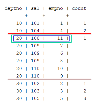
-
After
COUNTprocesses the partition's first row, it resets the current row to the partition's second row. The window now spans the current row and the row above it, soCOUNTreturns a value of 2: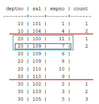
-
After
COUNTprocesses the partition's second row, it resets the current row to the partition's third row. The window now spans the current row and the two rows above it, soCOUNTreturns a value of 3: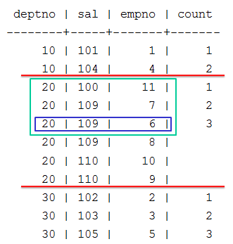
-
Thereafter,
COUNTcontinues to process the remaining partition rows and moves the window accordingly, but the window dimensions (ROWS BETWEEN 2 PRECEDING AND CURRENT ROW) remain unchanged as three rows. Accordingly, the value in thecountcolumn also remains unchanged (3):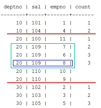
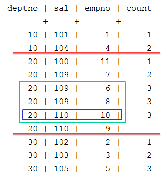
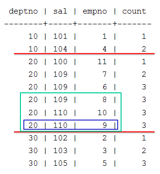
5.5.2 - Windows with a logical offset (RANGE)
The RANGE keyword defines an analytic window frame as a logical offset from the current row.
The RANGE keyword defines an analytic window frame as a logical offset from the current row.
Note
The value returned by an analytic function with a logical offset is always deterministic.For each row, an analytic function uses the window order clause (ORDER_BY) column or expression to calculate window frame dimensions as follows:
-
Within the current partition, evaluates the
ORDER_BYvalue of the current row against theORDER_BYvalues of contiguous rows. -
Determines which of these rows satisfy the specified range requirements relative to the current row.
-
Creates a window frame that includes only those rows.
-
Executes on the current window.
Example
This example uses the table property_sales, which contains data about neighborhood home sales:
=> SELECT property_key, neighborhood, sell_price FROM property_sales ORDER BY neighborhood, sell_price;
property_key | neighborhood | sell_price
--------------+---------------+------------
10918 | Jamaica Plain | 353000
10921 | Jamaica Plain | 450000
10927 | Jamaica Plain | 450000
10922 | Jamaica Plain | 474000
10919 | Jamaica Plain | 515000
10917 | Jamaica Plain | 675000
10924 | Jamaica Plain | 675000
10920 | Jamaica Plain | 705000
10923 | Jamaica Plain | 710000
10926 | Jamaica Plain | 875000
10925 | Jamaica Plain | 900000
10930 | Roslindale | 300000
10928 | Roslindale | 422000
10932 | Roslindale | 450000
10929 | Roslindale | 485000
10931 | Roslindale | 519000
10938 | West Roxbury | 479000
10933 | West Roxbury | 550000
10937 | West Roxbury | 550000
10934 | West Roxbury | 574000
10935 | West Roxbury | 598000
10936 | West Roxbury | 615000
10939 | West Roxbury | 720000
(23 rows)
The analytic function AVG can obtain the average of proximate selling prices within each neighborhood. The following query calculates for each home the average sale for all other neighborhood homes whose selling price was $50k higher or lower:
=> SELECT property_key, neighborhood, sell_price, AVG(sell_price) OVER(
PARTITION BY neighborhood ORDER BY sell_price
RANGE BETWEEN 50000 PRECEDING and 50000 FOLLOWING)::int AS comp_sales
FROM property_sales ORDER BY neighborhood;
property_key | neighborhood | sell_price | comp_sales
--------------+---------------+------------+------------
10918 | Jamaica Plain | 353000 | 353000
10927 | Jamaica Plain | 450000 | 458000
10921 | Jamaica Plain | 450000 | 458000
10922 | Jamaica Plain | 474000 | 472250
10919 | Jamaica Plain | 515000 | 494500
10917 | Jamaica Plain | 675000 | 691250
10924 | Jamaica Plain | 675000 | 691250
10920 | Jamaica Plain | 705000 | 691250
10923 | Jamaica Plain | 710000 | 691250
10926 | Jamaica Plain | 875000 | 887500
10925 | Jamaica Plain | 900000 | 887500
10930 | Roslindale | 300000 | 300000
10928 | Roslindale | 422000 | 436000
10932 | Roslindale | 450000 | 452333
10929 | Roslindale | 485000 | 484667
10931 | Roslindale | 519000 | 502000
10938 | West Roxbury | 479000 | 479000
10933 | West Roxbury | 550000 | 568000
10937 | West Roxbury | 550000 | 568000
10934 | West Roxbury | 574000 | 577400
10935 | West Roxbury | 598000 | 577400
10936 | West Roxbury | 615000 | 595667
10939 | West Roxbury | 720000 | 720000
(23 rows)
AVG processes this query as follows:
-
AVGevaluates row 1 of the first partition (Jamaica Plain), but finds no sales within $50k of this row'ssell_price, ($353k).AVGcreates a window that includes this row only, and returns an average of 353k for row 1: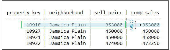
-
AVGevaluates row 2 and finds threesell_pricevalues within $50k of the current row.AVGcreates a window that includes these three rows, and returns an average of 458k for row 2: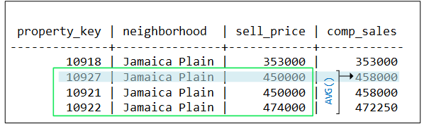
-
AVGevaluates row 3 and finds the same threesell_pricevalues within $50k of the current row.AVGcreates a window identical to the one before, and returns the same average of 458k for row 3: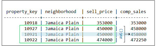
-
AVGevaluates row 4 and finds foursell_pricevalues within $50k of the current row.AVGexpands its window to include rows 2 through 5, and returns an average of $472.25k for row 4: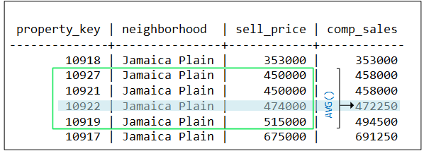
-
In similar fashion,
AVGevaluates the remaining rows in this partition. When the function evaluates the first row of the second partition (Roslindale), it resets the window as follows: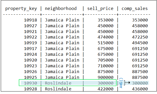
Restrictions
If RANGE specifies a constant value, that value's data type and the window's ORDER BY data type must be the same. The following exceptions apply:
-
RANGEcan specifyINTERVAL Year to Monthif the window order clause data type is one of following:TIMESTAMP,TIMESTAMP WITH TIMEZONE, orDATE.TIMEandTIME WITH TIMEZONEare not supported. -
RANGEcan specifyINTERVAL Day to Secondif the window order clause data is one of following:TIMESTAMP,TIMESTAMP WITH TIMEZONE,DATE,TIME, orTIME WITH TIMEZONE.
The window order clause must specify one of the following data types: NUMERIC, DATE/TIME, FLOAT or INTEGER. This requirement is ignored if the window specifies one of following frames:
-
RANGE BETWEEN UNBOUNDED PRECEDING AND CURRENT ROW -
RANGE BETWEEN CURRENT ROW AND UNBOUNDED FOLLOWING -
RANGE BETWEEN UNBOUNDED PRECEDING AND UNBOUNDED FOLLOWING
5.5.3 - Reporting aggregates
Some of the analytic functions that take the window-frame-clause are the reporting aggregates.
Some of the analytic functions that take the window-frame-clause are the reporting aggregates. These functions let you compare a partition's aggregate values with detail rows, taking the place of correlated subqueries or joins.
-
VARIANCE(), VAR_POP(), and VAR_SAMP()
If you use a window aggregate with an empty OVER() clause, the analytic function is used as a reporting function, where the entire input is treated as a single partition.
About standard deviation and variance functions
With standard deviation functions, a low standard deviation indicates that the data points tend to be very close to the mean, whereas high standard deviation indicates that the data points are spread out over a large range of values.
Standard deviation is often graphed and a distributed standard deviation creates the classic bell curve.
Variance functions measure how far a set of numbers is spread out.
Examples
Think of the window for reporting aggregates as a window defined as UNBOUNDED PRECEDING and UNBOUNDED FOLLOWING. The omission of a window-order-clause makes all rows in the partition also the window (reporting aggregates).
=> SELECT deptno, sal, empno, COUNT(sal)
OVER (PARTITION BY deptno) AS COUNT FROM emp;
deptno | sal | empno | count
--------+-----+-------+-------
10 | 101 | 1 | 2
10 | 104 | 4 | 2
------------------------------
20 | 110 | 10 | 6
20 | 110 | 9 | 6
20 | 109 | 7 | 6
20 | 109 | 6 | 6
20 | 109 | 8 | 6
20 | 100 | 11 | 6
------------------------------
30 | 105 | 5 | 3
30 | 103 | 3 | 3
30 | 102 | 2 | 3
(11 rows)
If the OVER() clause in the above query contained a window-order-clause (for example, ORDER BY sal), it would become a moving window (window aggregate) query with a default window of RANGE BETWEEN UNBOUNDED PRECEDING AND CURRENT ROW:
=> SELECT deptno, sal, empno, COUNT(sal) OVER (PARTITION BY deptno ORDER BY sal) AS COUNT FROM emp;
deptno | sal | empno | count
--------+-----+-------+-------
10 | 101 | 1 | 1
10 | 104 | 4 | 2
------------------------------
20 | 100 | 11 | 1
20 | 109 | 7 | 4
20 | 109 | 6 | 4
20 | 109 | 8 | 4
20 | 110 | 10 | 6
20 | 110 | 9 | 6
------------------------------
30 | 102 | 2 | 1
30 | 103 | 3 | 2
30 | 105 | 5 | 3
(11 rows)
What about LAST_VALUE?
You might wonder why you couldn't just use the LAST_VALUE() analytic function.
For example, for each employee, get the highest salary in the department:
=> SELECT deptno, sal, empno,LAST_VALUE(empno) OVER (PARTITION BY deptno ORDER BY sal) AS lv FROM emp;

Due to default window semantics, LAST_VALUE does not always return the last value of a partition. If you omit the window-frame-clause from the analytic clause, LAST_VALUE operates on this default window. Results, therefore, can seem non-intuitive because the function does not return the bottom of the current partition. It returns the bottom of the window, which continues to change along with the current input row being processed.
Remember the default window:
OVER (PARTITION BY deptno ORDER BY sal)
is the same as:
OVER(PARTITION BY deptno ORDER BY salROWS BETWEEN UNBOUNDED PRECEDING AND CURRENT ROW)
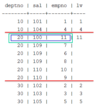 |
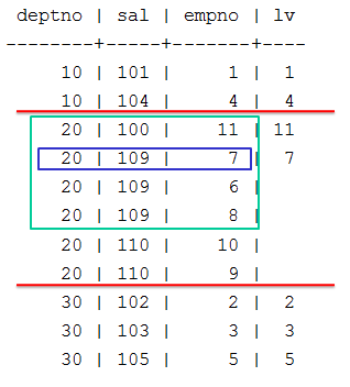 |
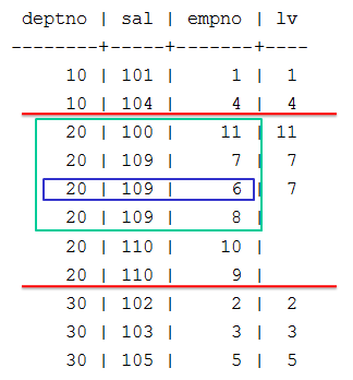 |
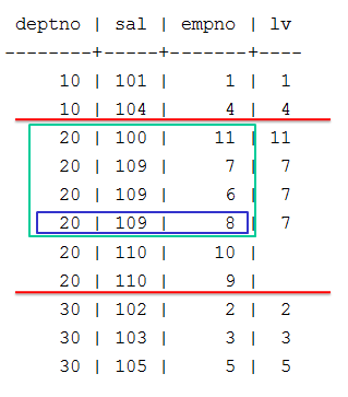 |
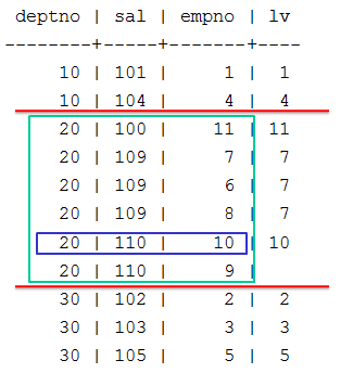 |
 |
If you want to return the last value of a partition, use UNBOUNDED PRECEDING AND UNBOUNDED FOLLOWING.
=> SELECT deptno, sal, empno, LAST_VALUE(empno)
OVER (PARTITION BY deptno ORDER BY sal
ROWS BETWEEN UNBOUNDED PRECEDING AND UNBOUNDED FOLLOWING) AS lv
FROM emp;

Vertica recommends that you use LAST_VALUE with the window-order-clause to produce deterministic results.
In the following example, empno 6, 7, and 8 have the same salary, so they are in adjacent rows. empno 8 appears first in this case but the order is not guaranteed.
Notice in the output above, the last value is 7, which is the last row from the partition deptno = 20. If the rows have a different order, then the function returns a different value:
Now the last value is 6, which is the last row from the partition deptno = 20. The solution is to add a unique key to the sort order. Even if the order of the query changes, the result will always be the same, and so deterministic.
=> SELECT deptno, sal, empno, LAST_VALUE(empno)
OVER (PARTITION BY deptno ORDER BY sal, empno
ROWS BETWEEN UNBOUNDED PRECEDING AND UNBOUNDED FOLLOWING) as lv
FROM emp;
Notice how the rows are now ordered by empno, the last value stays at 8, and it does not matter the order of the query.
5.6 - Named windows
An analytic function's OVER clause can reference a named window, which encapsulates one or more window clauses: a window partition (PARTITION BY) clause and (optionally) a window order (ORDER BY) clause.
An analytic function's OVER clause can reference a named window, which encapsulates one or more window clauses: a window partition (PARTITION BY) clause and (optionally) a window order (ORDER BY) clause. Named windows can be useful when you write queries that invoke multiple analytic functions with similar OVER clause syntax—for example, they use the same partition clauses.
A query names a window as follows:
WINDOW window‑name AS ( window-partition-clause [window-order-clause] );
The same query can name and reference multiple windows. All window names must be unique within the same query.
Examples
The following query invokes two analytic functions,
RANK and
DENSE_RANK. Because the two functions use the same partition and order clauses, the query names a window w that specifies both clauses. The two functions reference this window as follows:
=> SELECT employee_region region, employee_key, annual_salary,
RANK() OVER w Rank,
DENSE_RANK() OVER w "Dense Rank"
FROM employee_dimension WINDOW w AS (PARTITION BY employee_region ORDER BY annual_salary);
region | employee_key | annual_salary | Rank | Dense Rank
----------------------------------+--------------+---------------+------+------------
West | 5248 | 1200 | 1 | 1
West | 6880 | 1204 | 2 | 2
West | 5700 | 1214 | 3 | 3
West | 9857 | 1218 | 4 | 4
West | 6014 | 1218 | 4 | 4
West | 9221 | 1220 | 6 | 5
West | 7646 | 1222 | 7 | 6
West | 6621 | 1222 | 7 | 6
West | 6488 | 1224 | 9 | 7
West | 7659 | 1226 | 10 | 8
West | 7432 | 1226 | 10 | 8
West | 9905 | 1226 | 10 | 8
West | 9021 | 1228 | 13 | 9
West | 7855 | 1228 | 13 | 9
West | 7119 | 1230 | 15 | 10
...
If the named window omits an order clause, the query's OVER clauses can specify their own order clauses. For example, you can modify the previous query so each function uses a different order clause. The named window is defined so it includes only a partition clause:
=> SELECT employee_region region, employee_key, annual_salary,
RANK() OVER (w ORDER BY annual_salary DESC) Rank,
DENSE_RANK() OVER (w ORDER BY annual_salary ASC) "Dense Rank"
FROM employee_dimension WINDOW w AS (PARTITION BY employee_region);
region | employee_key | annual_salary | Rank | Dense Rank
----------------------------------+--------------+---------------+------+------------
West | 5248 | 1200 | 2795 | 1
West | 6880 | 1204 | 2794 | 2
West | 5700 | 1214 | 2793 | 3
West | 6014 | 1218 | 2791 | 4
West | 9857 | 1218 | 2791 | 4
West | 9221 | 1220 | 2790 | 5
West | 6621 | 1222 | 2788 | 6
West | 7646 | 1222 | 2788 | 6
West | 6488 | 1224 | 2787 | 7
West | 7432 | 1226 | 2784 | 8
West | 9905 | 1226 | 2784 | 8
West | 7659 | 1226 | 2784 | 8
West | 7855 | 1228 | 2782 | 9
West | 9021 | 1228 | 2782 | 9
West | 7119 | 1230 | 2781 | 10
...
Similarly, an OVER clause specifies a named window can also specify a window frame clause, provided the named window includes an order clause. This can be useful inasmuch as you cannot define a named windows to include a window frame clause.
For example, the following query defines a window that encapsulates partitioning and order clauses. The OVER clause invokes this window and also includes a window frame clause:
=> SELECT deptno, sal, empno, COUNT(*) OVER (w ROWS BETWEEN 2 PRECEDING AND CURRENT ROW) AS count
FROM emp WINDOW w AS (PARTITION BY deptno ORDER BY sal);
deptno | sal | empno | count
--------+-----+-------+-------
10 | 101 | 1 | 1
10 | 104 | 4 | 2
20 | 100 | 11 | 1
20 | 109 | 8 | 2
20 | 109 | 6 | 3
20 | 109 | 7 | 3
20 | 110 | 10 | 3
20 | 110 | 9 | 3
30 | 102 | 2 | 1
30 | 103 | 3 | 2
30 | 105 | 5 | 3
(11 rows)
Recursive window references
A WINDOW clause can reference another window that is already named. For example, because named window w1 is defined before w2, the WINDOW clause that defines w2 can reference w1:
=> SELECT RANK() OVER(w1 ORDER BY sal DESC), RANK() OVER w2
FROM EMP WINDOW w1 AS (PARTITION BY deptno), w2 AS (w1 ORDER BY sal);
Restrictions
-
An
OVERclause can reference only one named window. -
Each
WINDOWclause within the same query must have a unique name.
5.7 - Analytic query examples
The topics in this section show how to use analytic queries for calculations.
The topics in this section show how to use analytic queries for calculations.
5.7.1 - Calculating a median value
A median is a numerical value that separates the higher half of a sample from the lower half.
A median is a numerical value that separates the higher half of a sample from the lower half. For example, you can retrieve the median of a finite list of numbers by arranging all observations from lowest value to highest value and then picking the middle one.
If the number of observations is even, then there is no single middle value; the median is the mean (average) of the two middle values.
The following example uses this table:
CREATE TABLE allsales(state VARCHAR(20), name VARCHAR(20), sales INT);
INSERT INTO allsales VALUES('MA', 'A', 60);
INSERT INTO allsales VALUES('NY', 'B', 20);
INSERT INTO allsales VALUES('NY', 'C', 15);
INSERT INTO allsales VALUES('MA', 'D', 20);
INSERT INTO allsales VALUES('MA', 'E', 50);
INSERT INTO allsales VALUES('NY', 'F', 40);
INSERT INTO allsales VALUES('MA', 'G', 10);
COMMIT;
You can use the analytic function
MEDIAN to calculate the median of all sales in this table. In the following query, the function's OVER clause is empty, so the query returns the same aggregated value for each row of the result set:
=> SELECT name, sales, MEDIAN(sales) OVER() AS median FROM allsales;
name | sales | median
------+-------+--------
G | 10 | 20
C | 15 | 20
D | 20 | 20
B | 20 | 20
F | 40 | 20
E | 50 | 20
A | 60 | 20
(7 rows)
You can modify this query to group sales by state and obtain the median for each one. To do so, include a window partition clause in the OVER clause:
=> SELECT state, name, sales, MEDIAN(sales) OVER(partition by state) AS median FROM allsales;
state | name | sales | median
-------+------+-------+--------
MA | G | 10 | 35
MA | D | 20 | 35
MA | E | 50 | 35
MA | A | 60 | 35
NY | C | 15 | 20
NY | B | 20 | 20
NY | F | 40 | 20
(7 rows)
5.7.2 - Getting price differential for two stocks
The following subquery selects out two stocks of interest.
The following subquery selects out two stocks of interest. The outer query uses the LAST_VALUE() and OVER() components of analytics, with IGNORE NULLS.
Schema
DROP TABLE Ticks CASCADE;
CREATE TABLE Ticks (ts TIMESTAMP, Stock varchar(10), Bid float);
INSERT INTO Ticks VALUES('2011-07-12 10:23:54', 'abc', 10.12);
INSERT INTO Ticks VALUES('2011-07-12 10:23:58', 'abc', 10.34);
INSERT INTO Ticks VALUES('2011-07-12 10:23:59', 'abc', 10.75);
INSERT INTO Ticks VALUES('2011-07-12 10:25:15', 'abc', 11.98);
INSERT INTO Ticks VALUES('2011-07-12 10:25:16', 'abc');
INSERT INTO Ticks VALUES('2011-07-12 10:25:22', 'xyz', 45.16);
INSERT INTO Ticks VALUES('2011-07-12 10:25:27', 'xyz', 49.33);
INSERT INTO Ticks VALUES('2011-07-12 10:31:12', 'xyz', 65.25);
INSERT INTO Ticks VALUES('2011-07-12 10:31:15', 'xyz');
COMMIT;
Ticks table
=> SELECT * FROM ticks;
ts | stock | bid
---------------------+-------+-------
2011-07-12 10:23:59 | abc | 10.75
2011-07-12 10:25:22 | xyz | 45.16
2011-07-12 10:23:58 | abc | 10.34
2011-07-12 10:25:27 | xyz | 49.33
2011-07-12 10:23:54 | abc | 10.12
2011-07-12 10:31:15 | xyz |
2011-07-12 10:25:15 | abc | 11.98
2011-07-12 10:25:16 | abc |
2011-07-12 10:31:12 | xyz | 65.25
(9 rows)
Query
=> SELECT ts, stock, bid, last_value(price1 IGNORE NULLS)
OVER(ORDER BY ts) - last_value(price2 IGNORE NULLS)
OVER(ORDER BY ts) as price_diff
FROM
(SELECT ts, stock, bid,
CASE WHEN stock = 'abc' THEN bid ELSE NULL END AS price1,
CASE WHEN stock = 'xyz' then bid ELSE NULL END AS price2
FROM ticks
WHERE stock IN ('abc','xyz')
) v1
ORDER BY ts;
ts | stock | bid | price_diff
---------------------+-------+-------+------------
2011-07-12 10:23:54 | abc | 10.12 |
2011-07-12 10:23:58 | abc | 10.34 |
2011-07-12 10:23:59 | abc | 10.75 |
2011-07-12 10:25:15 | abc | 11.98 |
2011-07-12 10:25:16 | abc | |
2011-07-12 10:25:22 | xyz | 45.16 | -33.18
2011-07-12 10:25:27 | xyz | 49.33 | -37.35
2011-07-12 10:31:12 | xyz | 65.25 | -53.27
2011-07-12 10:31:15 | xyz | | -53.27
(9 rows)
5.7.3 - Calculating the moving average
Calculating the moving average is useful to get an estimate about the trends in a data set.
Calculating the moving average is useful to get an estimate about the trends in a data set. The moving average is the average of any subset of numbers over a period of time. For example, if you have retail data that spans over ten years, you could calculate a three year moving average, a four year moving average, and so on. This example calculates a 40-second moving average of bids for one stock. This examples uses the
ticks table schema.
Query
=> SELECT ts, bid, AVG(bid)
OVER(ORDER BY ts
RANGE BETWEEN INTERVAL '40 seconds'
PRECEDING AND CURRENT ROW)
FROM ticks
WHERE stock = 'abc'
GROUP BY bid, ts
ORDER BY ts;
ts | bid | ?column?
---------------------+-------+------------------
2011-07-12 10:23:54 | 10.12 | 10.12
2011-07-12 10:23:58 | 10.34 | 10.23
2011-07-12 10:23:59 | 10.75 | 10.4033333333333
2011-07-12 10:25:15 | 11.98 | 11.98
2011-07-12 10:25:16 | | 11.98
(5 rows)
DROP TABLE Ticks CASCADE;
CREATE TABLE Ticks (ts TIMESTAMP, Stock varchar(10), Bid float);
INSERT INTO Ticks VALUES('2011-07-12 10:23:54', 'abc', 10.12);
INSERT INTO Ticks VALUES('2011-07-12 10:23:58', 'abc', 10.34);
INSERT INTO Ticks VALUES('2011-07-12 10:23:59', 'abc', 10.75);
INSERT INTO Ticks VALUES('2011-07-12 10:25:15', 'abc', 11.98);
INSERT INTO Ticks VALUES('2011-07-12 10:25:16', 'abc');
INSERT INTO Ticks VALUES('2011-07-12 10:25:22', 'xyz', 45.16);
INSERT INTO Ticks VALUES('2011-07-12 10:25:27', 'xyz', 49.33);
INSERT INTO Ticks VALUES('2011-07-12 10:31:12', 'xyz', 65.25);
INSERT INTO Ticks VALUES('2011-07-12 10:31:15', 'xyz');
COMMIT;
5.7.4 - Getting latest bid and ask results
The following query fills in missing NULL values to create a full book order showing latest bid and ask price and size, by vendor id.
The following query fills in missing NULL values to create a full book order showing latest bid and ask price and size, by vendor id. Original rows have values for (typically) one price and one size, so use last_value with "ignore nulls" to find the most recent non-null value for the other pair each time there is an entry for the ID. Sequenceno provides a unique total ordering.
Schema:
=> CREATE TABLE bookorders(
vendorid VARCHAR(100),
date TIMESTAMP,
sequenceno INT,
askprice FLOAT,
asksize INT,
bidprice FLOAT,
bidsize INT);
=> INSERT INTO bookorders VALUES('3325XPK','2011-07-12 10:23:54', 1, 10.12, 55, 10.23, 59);
=> INSERT INTO bookorders VALUES('3345XPZ','2011-07-12 10:23:55', 2, 10.55, 58, 10.75, 57);
=> INSERT INTO bookorders VALUES('445XPKF','2011-07-12 10:23:56', 3, 10.22, 43, 54);
=> INSERT INTO bookorders VALUES('445XPKF','2011-07-12 10:23:57', 3, 10.22, 59, 10.25, 61);
=> INSERT INTO bookorders VALUES('3425XPY','2011-07-12 10:23:58', 4, 11.87, 66, 11.90, 66);
=> INSERT INTO bookorders VALUES('3727XVK','2011-07-12 10:23:59', 5, 11.66, 51, 11.67, 62);
=> INSERT INTO bookorders VALUES('5325XYZ','2011-07-12 10:24:01', 6, 15.05, 44, 15.10, 59);
=> INSERT INTO bookorders VALUES('3675XVS','2011-07-12 10:24:05', 7, 15.43, 47, 58);
=> INSERT INTO bookorders VALUES('8972VUG','2011-07-12 10:25:15', 8, 14.95, 52, 15.11, 57);
COMMIT;
Query:
=> SELECT
sequenceno Seq,
date "Time",
vendorid ID,
LAST_VALUE (bidprice IGNORE NULLS)
OVER (PARTITION BY vendorid ORDER BY sequenceno
ROWS BETWEEN UNBOUNDED PRECEDING AND CURRENT ROW)
AS "Bid Price",
LAST_VALUE (bidsize IGNORE NULLS)
OVER (PARTITION BY vendorid ORDER BY sequenceno
ROWS BETWEEN UNBOUNDED PRECEDING AND CURRENT ROW)
AS "Bid Size",
LAST_VALUE (askprice IGNORE NULLS)
OVER (PARTITION BY vendorid ORDER BY sequenceno
ROWS BETWEEN UNBOUNDED PRECEDING AND CURRENT ROW)
AS "Ask Price",
LAST_VALUE (asksize IGNORE NULLS)
OVER (PARTITION BY vendorid order by sequenceno
ROWS BETWEEN UNBOUNDED PRECEDING AND CURRENT ROW )
AS "Ask Size"
FROM bookorders
ORDER BY sequenceno;
Seq | Time | ID | Bid Price | Bid Size | Ask Price | Ask Size
-----+---------------------+---------+-----------+----------+-----------+----------
1 | 2011-07-12 10:23:54 | 3325XPK | 10.23 | 59 | 10.12 | 55
2 | 2011-07-12 10:23:55 | 3345XPZ | 10.75 | 57 | 10.55 | 58
3 | 2011-07-12 10:23:57 | 445XPKF | 10.25 | 61 | 10.22 | 59
3 | 2011-07-12 10:23:56 | 445XPKF | 54 | | 10.22 | 43
4 | 2011-07-12 10:23:58 | 3425XPY | 11.9 | 66 | 11.87 | 66
5 | 2011-07-12 10:23:59 | 3727XVK | 11.67 | 62 | 11.66 | 51
6 | 2011-07-12 10:24:01 | 5325XYZ | 15.1 | 59 | 15.05 | 44
7 | 2011-07-12 10:24:05 | 3675XVS | 58 | | 15.43 | 47
8 | 2011-07-12 10:25:15 | 8972VUG | 15.11 | 57 | 14.95 | 52
(9 rows)
5.8 - Event-based windows
Add index entries.
Event-based windows let you break time series data into windows that border on significant events within the data. This is especially relevant in financial data where analysis often focuses on specific events as triggers to other activity.
Vertica provides two event-based window functions that are not part of the SQL-99 standard:
-
CONDITIONAL_CHANGE_EVENTassigns an event window number to each row, starting from 0, and increments by 1 when the result of evaluating the argument expression on the current row differs from that on the previous row. This function is similar to the analytic functionROW_NUMBER, which assigns a unique number, sequentially, starting from 1, to each row within a partition. -
CONDITIONAL_TRUE_EVENTassigns an event window number to each row, starting from 0, and increments the number by 1 when the result of the boolean argument expression evaluates true.
Both functions are described in greater detail below.
Example schema
The examples on this page use the following schema:
CREATE TABLE TickStore3 (ts TIMESTAMP, symbol VARCHAR(8), bid FLOAT);
CREATE PROJECTION TickStore3_p (ts, symbol, bid) AS SELECT * FROM TickStore3 ORDER BY ts, symbol, bid UNSEGMENTED ALL NODES;
INSERT INTO TickStore3 VALUES ('2009-01-01 03:00:00', 'XYZ', 10.0);
INSERT INTO TickStore3 VALUES ('2009-01-01 03:00:03', 'XYZ', 11.0);
INSERT INTO TickStore3 VALUES ('2009-01-01 03:00:06', 'XYZ', 10.5);
INSERT INTO TickStore3 VALUES ('2009-01-01 03:00:09', 'XYZ', 11.0);
COMMIT;
Using CONDITIONAL_CHANGE_EVENT
The analytical function CONDITIONAL_CHANGE_EVENT returns a sequence of integers indicating event window numbers, starting from 0. The function increments the event window number when the result of evaluating the function expression on the current row differs from the previous value.
In the following example, the first query returns all records from the TickStore3 table. The second query uses the CONDITIONAL_CHANGE_EVENT function on the bid column. Since each bid row value is different from the previous value, the function increments the window ID from 0 to 3:
SELECT ts, symbol, bidFROM Tickstore3 ORDER BY ts; |
| |
|
==> |
ts | symbol | bid | cce ---------------------+--------+------+----- 2009-01-01 03:00:00 | XYZ | 10 | 0 2009-01-01 03:00:03 | XYZ | 11 | 1 2009-01-01 03:00:06 | XYZ | 10.5 | 2 2009-01-01 03:00:09 | XYZ | 11 | 3 (4 rows) |
The following figure is a graphical illustration of the change in the bid price. Each value is different from its previous one, so the window ID increments for each time slice:
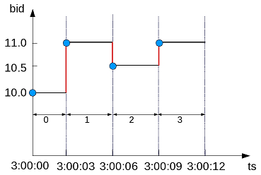
So the window ID starts at 0 and increments at every change in from the previous value.
In this example, the bid price changes from $10 to $11 in the second row, but then stays the same. CONDITIONAL_CHANGE_EVENT increments the event window ID in row 2, but not subsequently:
SELECT ts, symbol, bidFROM Tickstore3 ORDER BY ts; |
| |
|
==> |
ts | symbol | bid | cce ---------------------+--------+------+----- 2009-01-01 03:00:00 | XYZ | 10 | 0 2009-01-01 03:00:03 | XYZ | 11 | 1 2009-01-01 03:00:06 | XYZ | 11 | 1 2009-01-01 03:00:09 | XYZ | 11 | 1 |
The following figure is a graphical illustration of the change in the bid price at 3:00:03 only. The price stays the same at 3:00:06 and 3:00:09, so the window ID remains at 1 for each time slice after the change:

Using CONDITIONAL_TRUE_EVENT
Like CONDITIONAL_CHANGE_EVENT, the analytic function CONDITIONAL_TRUE_EVENT also returns a sequence of integers indicating event window numbers, starting from 0. The two functions differ as follows:
-
CONDITIONAL_TRUE_EVENTincrements the window ID each time its expression evaluates to true. -
CONDITIONAL_CHANGE_EVENTincrements on a comparison expression with the previous value.
In the following example, the first query returns all records from the TickStore3 table. The second query uses CONDITIONAL_TRUE_EVENT to test whether the current bid is greater than a given value (10.6). Each time the expression tests true, the function increments the window ID. The first time the function increments the window ID is on row 2, when the value is 11. The expression tests false for the next row (value is not greater than 10.6), so the function does not increment the event window ID. In the final row, the expression is true for the given condition, and the function increments the window:
SELECT ts, symbol, bidFROM Tickstore3 ORDER BY ts; |
| |
|
==> |
ts | symbol | bid | cte---------------------+--------+------+----- 2009-01-01 03:00:00 | XYZ | 10 | 0 2009-01-01 03:00:03 | XYZ | 11 | 1 2009-01-01 03:00:06 | XYZ | 10.5 | 1 2009-01-01 03:00:09 | XYZ | 11 | 2 |
The following figure is a graphical illustration that shows the bid values and window ID changes. Because the bid value is greater than $10.6 on only the second and fourth time slices (3:00:03 and 3:00:09), the window ID returns <0,1,1,2>:
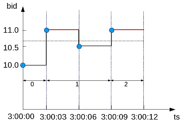
In the following example, the first query returns all records from the TickStore3 table, ordered by the tickstore values (ts). The second query uses CONDITIONAL_TRUE_EVENT to increment the window ID each time the bid value is greater than 10.6. The first time the function increments the event window ID is on row 2, where the value is 11. The window ID then increments each time after that, because the expression (bid > 10.6) tests true for each time slice:
SELECT ts, symbol, bidFROM Tickstore3 ORDER BY ts; |
| |
|
==> |
ts | symbol | bid | cte ---------------------+--------+------+----- 2009-01-01 03:00:00 | XYZ | 10 | 0 2009-01-01 03:00:03 | XYZ | 11 | 1 2009-01-01 03:00:06 | XYZ | 11 | 2 2009-01-01 03:00:09 | XYZ | 11 | 3 |
The following figure is a graphical illustration that shows the bid values and window ID changes. The bid value is greater than 10.6 on the second time slice (3:00:03) and remains for the remaining two time slices. The function increments the event window ID each time because the expression tests true:
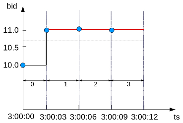
Advanced use of event-based windows
In event-based window functions, the condition expression accesses values from the current row only. To access a previous value, you can use a more powerful event-based window that allows the window event condition to include previous data points. For example, analytic function LAG(x, n) retrieves the value of column x in the nth to last input record. In this case, LAG shares the OVER specifications of the CONDITIONAL_CHANGE_EVENT or CONDITIONAL_TRUE_EVENT function expression.
In the following example, the first query returns all records from the TickStore3 table. The second query uses CONDITIONAL_TRUE_EVENT with the LAG function in its boolean expression. In this case, CONDITIONAL_TRUE_EVENT increments the event window ID each time the bid value on the current row is less than the previous value. The first time CONDITIONAL_TRUE_EVENT increments the window ID starts on the third time slice, when the expression tests true. The current value (10.5) is less than the previous value. The window ID is not incremented in the last row because the final value is greater than the previous row:
SELECT ts, symbol, bidFROM Tickstore3 ORDER BY ts; |
|
|
ts | symbol | bid | cte ---------------------+--------+------+----- 2009-01-01 03:00:00 | XYZ | 10 | 0 2009-01-01 03:00:03 | XYZ | 11 | 0 2009-01-01 03:00:06 | XYZ | 10.5 | 1 2009-01-01 03:00:09 | XYZ | 11 | 1 |
The following figure illustrates the second query above. When the bid price is less than the previous value, the window ID gets incremented, which occurs only in the third time slice (3:00:06):
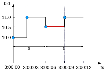
See also
5.9 - Sessionization with event-based windows
Sessionization, a special case of event-based windows, is a feature often used to analyze click streams, such as identifying web browsing sessions from recorded web clicks.
Sessionization, a special case of event-based windows, is a feature often used to analyze click streams, such as identifying web browsing sessions from recorded web clicks.
In Vertica, given an input clickstream table, where each row records a Web page click made by a particular user (or IP address), the sessionization computation attempts to identify Web browsing sessions from the recorded clicks by grouping the clicks from each user based on the time-intervals between the clicks. If two clicks from the same user are made too far apart in time, as defined by a time-out threshold, the clicks are treated as though they are from two different browsing sessions.
Example Schema The examples in this topic use the following WebClicks schema to represent a simple clickstream table:
CREATE TABLE WebClicks(userId INT, timestamp TIMESTAMP);
INSERT INTO WebClicks VALUES (1, '2009-12-08 3:00:00 pm');
INSERT INTO WebClicks VALUES (1, '2009-12-08 3:00:25 pm');
INSERT INTO WebClicks VALUES (1, '2009-12-08 3:00:45 pm');
INSERT INTO WebClicks VALUES (1, '2009-12-08 3:01:45 pm');
INSERT INTO WebClicks VALUES (2, '2009-12-08 3:02:45 pm');
INSERT INTO WebClicks VALUES (2, '2009-12-08 3:02:55 pm');
INSERT INTO WebClicks VALUES (2, '2009-12-08 3:03:55 pm');
COMMIT;
The input table WebClicks contains the following rows:
=> SELECT * FROM WebClicks;
userId | timestamp
--------+---------------------
1 | 2009-12-08 15:00:00
1 | 2009-12-08 15:00:25
1 | 2009-12-08 15:00:45
1 | 2009-12-08 15:01:45
2 | 2009-12-08 15:02:45
2 | 2009-12-08 15:02:55
2 | 2009-12-08 15:03:55
(7 rows)
In the following query, sessionization performs computation on the SELECT list columns, showing the difference between the current and previous timestamp value using LAG(). It evaluates to true and increments the window ID when the difference is greater than 30 seconds.
=> SELECT userId, timestamp,
CONDITIONAL_TRUE_EVENT(timestamp - LAG(timestamp) > '30 seconds')
OVER(PARTITION BY userId ORDER BY timestamp) AS session FROM WebClicks;
userId | timestamp | session
--------+---------------------+---------
1 | 2009-12-08 15:00:00 | 0
1 | 2009-12-08 15:00:25 | 0
1 | 2009-12-08 15:00:45 | 0
1 | 2009-12-08 15:01:45 | 1
2 | 2009-12-08 15:02:45 | 0
2 | 2009-12-08 15:02:55 | 0
2 | 2009-12-08 15:03:55 | 1
(7 rows)
In the output, the session column contains the window ID from the CONDITIONAL_TRUE_EVENT function. The window ID evaluates to true on row 4 (timestamp 15:01:45), and the ID that follows row 4 is zero because it is the start of a new partition (for user ID 2), and that row does not evaluate to true until the last line in the output.
You might want to give users different time-out thresholds. For example, one user might have a slower network connection or be multi-tasking, while another user might have a faster connection and be focused on a single Web site, doing a single task.
To compute an adaptive time-out threshold based on the last 2 clicks, use CONDITIONAL_TRUE_EVENT with LAG to return the average time between the last 2 clicks with a grace period of 3 seconds:
=> SELECT userId, timestamp, CONDITIONAL_TRUE_EVENT(timestamp - LAG(timestamp) >
(LAG(timestamp, 1) - LAG(timestamp, 3)) / 2 + '3 seconds')
OVER(PARTITION BY userId ORDER BY timestamp) AS session
FROM WebClicks;
userId | timestamp | session
--------+---------------------+---------
2 | 2009-12-08 15:02:45 | 0
2 | 2009-12-08 15:02:55 | 0
2 | 2009-12-08 15:03:55 | 0
1 | 2009-12-08 15:00:00 | 0
1 | 2009-12-08 15:00:25 | 0
1 | 2009-12-08 15:00:45 | 0
1 | 2009-12-08 15:01:45 | 1
(7 rows)
Note
You cannot define a moving window in time series data. For example, if the query is evaluating the first row and there’s no data, it will be the current row. If you have a lag of 2, no results are returned until the third row.See also
6 - Machine learning for predictive analytics
Vertica provides a number of machine learning functions for performing in-database analysis.
Vertica provides a number of machine learning functions for performing in-database analysis. These functions perform data preparation, model training, and predictive tasks. Vertica supports the following in-database machine learning algorithms:
- Regression algorithms: Linear regression, random forest, SVM, XGBoost
- Classification algorithms: Logistic regression, naive Bayes, random forest, SVM, XGBoost
- Clustering algorithms: K-means, bisecting k-means
- Time series forecasting: Autoregression, moving-average
For a scikit-like machine learning library that integrates directly with the data in your Vertica database, see VerticaPy.
For more information about specific machine learning functions, see Machine learning functions.
6.1 - Download the machine learning example data
You need several data sets to run the machine learning examples.
You need several data sets to run the machine learning examples. You can download these data sets from the Vertica GitHub repository.
Important
The GitHub examples are based on the latest Vertica version. If you note differences, please upgrade to the latest version.You can download the example data in either of two ways:
-
Download the ZIP file. Extract the contents of the file into a directory.
-
Clone the Vertica Machine Learning GitHub repository. Using a terminal window, run the following command:
$ git clone https://github.com/vertica/Machine-Learning-Examples
Loading the example data
You can load the example data by doing one of the following. Note that models are not automatically dropped. You must either rerun the load_ml_data.sql script to drop models or manually drop them.
-
Copying and pasting the DDL and DML operations in
load_ml_data.sqlin a vsql prompt or another Vertica client. -
Running the following command from a terminal window within the data folder in the Machine-Learning-Examples directory:
$ /opt/vertica/bin/vsql -d <name of your database> -f load_ml_data.sql
You must also load the naive_bayes_data_prepration.sql script in the Machine-Learning-Examples directory:
$ /opt/vertica/bin/vsql -d <name of your database> -f ./naive_bayes/naive_bayes_data_preparation.sql
Example data descriptions
The repository contains the following data sets.
| Name | Description |
|---|---|
| agar_dish | Synthetic data set meant to represent clustering of bacteria on an agar dish. Contains the following columns: id, x-coordinate, and y-coordinate. |
| agar_dish_2 | 125 rows sampled randomly from the original 500 rows of the agar_dish data set. |
| agar_dish_1 | 375 rows sampled randomly from the original 500 rows of the agar_dish data set. |
| baseball | Contains statistics from a fictional baseball league. The statistics included are: first name, last name, date of birth, team name, homeruns, hits, batting average, and salary. |
| daily-min-temperatures | Contains data on the daily minimum temperature in Melbourne, Australia from 1981 through 1990. |
| dem_votes |
Contains data on the number of yes and no votes by Democrat members of U.S. Congress for each of the 16 votes in the house84 data set. The table must be populated by running the naive_bayes_data_prepration.sql script. Contains the following columns: vote, yes, no. |
| faithful |
Wait times between eruptions and the duration of the eruption for the Old Faithful geyser in Yellowstone National Park, Wyoming, USA. Reference Härdle, W. (1991) Smoothing Techniques with Implementation in S. New York: Springer. Azzalini, A. and Bowman, A. W. (1990). A look at some data on the Old Faithful geyser. Applied Statistics 39, 357–365. |
| faithful_testing | Roughly 60% of the original 272 rows of the faithful data set. |
| faithful_training | Roughly 40% of the original 272 rows of the faithful data set. |
| house84 |
The house84 data set includes votes for each of the U.S. House of Representatives Congress members on 16 votes. Contains the following columns: id, party, vote1, vote2, vote3, vote4, vote5, vote6, vote7, vote8, vote9, vote10, vote11, vote12, vote13, vote14, vote15, vote16. Reference Congressional Quarterly Almanac, 98th Congress, 2nd session 1984, Volume XL: Congressional Quarterly Inc. Washington, D.C., 1985. |
| iris |
The iris data set gives the measurements in centimeters of the variables sepal length and width and petal length and width, respectively, for 50 flowers from each of 3 species of iris. The species are Iris setosa, versicolor, and virginica. Reference Becker, R. A., Chambers, J. M. and Wilks, A. R. (1988) The New S Language. Wadsworth & Brooks/Cole. |
| iris1 | 90 rows sampled randomly from the original 150 rows in the iris data set. |
| iris2 | 60 rows sampled randomly from the original 150 rows in the iris data set. |
| mtcars |
The data was extracted from the 1974 Motor Trend US magazine, and comprises fuel consumption and 10 aspects of automobile design and performance for 32 automobiles (1973–74 models). Reference Henderson and Velleman (1981), Building multiple regression models interactively. Biometrics, 37, 391–411. |
| rep_votes |
Contains data on the number of yes and no votes by Republican members of U.S. Congress for each of the 16 votes in the house84 data set. The table must be populated by running the naive_bayes_data_prepration.sql script. Contains the following columns: vote, yes, no. |
| salary_data | Contains fictional employee data. The data included are: employee id, first name, last name, years worked, and current salary. |
| transaction_data | Contains fictional credit card transactions with a BOOLEAN column indicating whether there was fraud associated with the transaction. The data included are: first name, last name, store, cost, and fraud. |
| titanic_testing | Contains passenger information from the Titanic ship including sex, age, passenger class, and whether or not they survived. |
| titanic_training | Contains passenger information from the Titanic ship including sex, age, passenger class, and whether or not they survived. |
| world | Contains country-specific information about human development using HDI, GDP, and CO2 emissions. |
6.2 - Data preparation
Before you can analyze your data, you must prepare it.
Before you can analyze your data, you must prepare it. You can do the following data preparation tasks in Vertica:
6.2.1 - Balancing imbalanced data
Imbalanced data occurs when an uneven distribution of classes occurs in the data.
Imbalanced data occurs when an uneven distribution of classes occurs in the data. Building a predictive model on the imbalanced data set would cause a model that appears to yield high accuracy but does not generalize well to the new data in the minority class. To prevent creating models with false levels of accuracy, you should rebalance your imbalanced data before creating a predictive model.
Before you begin the example, load the Machine Learning sample data.You see imbalanced data a lot in financial transaction data where the majority of the transactions are not fraudulent and a small number of the transactions are fraudulent, as shown in the following example.
-
View the distribution of the classes.
=> SELECT fraud, COUNT(fraud) FROM transaction_data GROUP BY fraud; fraud | COUNT -------+------- TRUE | 19 FALSE | 981 (2 rows) -
Use the BALANCE function to create a more balanced data set.
=> SELECT BALANCE('balance_fin_data', 'transaction_data', 'fraud', 'under_sampling' USING PARAMETERS sampling_ratio = 0.2); BALANCE -------------------------- Finished in 1 iteration (1 row) -
View the new distribution of the classifiers.
=> SELECT fraud, COUNT(fraud) FROM balance_fin_data GROUP BY fraud; fraud | COUNT -------+------- t | 19 f | 236 (2 rows)
See also
6.2.2 - Detect outliers
Outliers are data points that greatly differ from other data points in a dataset.
Outliers are data points that greatly differ from other data points in a dataset. You can use outlier detection for applications such as fraud detection and system health monitoring, or you can detect outliers to then remove them from your data. If you leave outliers in your data when training a machine learning model, your resultant model is at risk for bias and skewed predictions. Vertica supports two methods for detecting outliers: the DETECT_OUTLIERS function and the IFOREST algorithm.
Note
The examples below use the baseball dataset from the machine learning example data. If you haven't already, Download the machine learning example data.Isolation forest
Isolation forest (iForest) is an unsupervised algorithm that operates on the assumption that outliers are few and different. This assumption makes outliers susceptible to a separation mechanism called isolation. Instead of comparing data instances to a constructed normal distribution of each data feature, isolation focuses on outliers themselves.
To isolate outliers directly, iForest builds binary tree structures named isolation trees (iTrees) to model the feature space. These iTrees randomly and recursively split the feature space so that each node of the tree represents a feature subspace. For instance, the first split divides the whole feature space into two subspaces, which are represented by the two child nodes of the root node. A data instance is considered isolated when it is the only member of a feature subspace. Because outliers are assumed to be few and different, outliers are likely to be isolated sooner than normal data instances.
In order to improve the robustness of the algorithm, iForest builds an ensemble of iTrees, which each separate the feature space differently. The algorithm calculates the average path length needed to isolate a data instance across all iTrees. This average path length helps determine the anomaly_score for each data instance in a dataset. The data instances with an anomaly_score above a given threshold are considered outliers.
You do not need a large dataset to train an iForest, and even a small sample should suffice to train an accurate model. The data can have columns of types CHAR, VARCHAR, BOOL, INT, or FLOAT.
After you have a trained an iForest model, you can use the APPLY_IFOREST function to detect outliers in any new data added to the dataset.
The following example demonstrates how to train an iForest model and detect outliers on the baseball dataset.
To build and train an iForest model, call IFOREST:
=> SELECT IFOREST('baseball_outliers','baseball','hr, hits, salary' USING PARAMETERS max_depth=30, nbins=100);
IFOREST
----------
Finished
(1 row)
You can view a summary of the trained model using GET_MODEL_SUMMARY:
=> SELECT GET_MODEL_SUMMARY(USING PARAMETERS model_name='baseball_outliers');
GET_MODEL_SUMMARY
---------------------------------------------------------------------------------------------------------------------------------------------
===========
call_string
===========
SELECT iforest('public.baseball_outliers', 'baseball', 'hr, hits, salary' USING PARAMETERS exclude_columns='', ntree=100, sampling_size=0.632,
col_sample_by_tree=1, max_depth=30, nbins=100);
=======
details
=======
predictor| type
---------+----------------
hr | int
hits | int
salary |float or numeric
===============
Additional Info
===============
Name |Value
------------------+-----
tree_count | 100
rejected_row_count| 0
accepted_row_count|1000
(1 row)
You can apply the trained iForest model to the baseball dataset with APPLY_IFOREST. To view only the data instances that are identified as outliers, you can run the following query:
=> SELECT * FROM (SELECT first_name, last_name, APPLY_IFOREST(hr, hits, salary USING PARAMETERS model_name='baseball_outliers', threshold=0.6)
AS predictions FROM baseball) AS outliers WHERE predictions.is_anomaly IS true;
first_name | last_name | predictions
------------+-----------+--------------------------------------------------------
Jacqueline | Richards | {"anomaly_score":0.8572338674053986,"is_anomaly":true}
Debra | Hall | {"anomaly_score":0.6007846156043213,"is_anomaly":true}
Gerald | Fuller | {"anomaly_score":0.6813650107767862,"is_anomaly":true}
(3 rows)
Instead of specifying a threshold value for APPLY_IFOREST, you can set the contamination parameter. This parameter sets a threshold so that the ratio of training data points labeled as outliers is approximately equal to the value of contamination:
=> SELECT * FROM (SELECT first_name, last_name, APPLY_IFOREST(team, hr, hits, avg, salary USING PARAMETERS model_name='baseball_anomalies',
contamination = 0.1) AS predictions FROM baseball) AS outliers WHERE predictions.is_anomaly IS true;
first_name | last_name | predictions
------------+-----------+--------------------------------------------------------
Marie | Fields | {"anomaly_score":0.5307715717521868,"is_anomaly":true}
Jacqueline | Richards | {"anomaly_score":0.777757463074347,"is_anomaly":true}
Debra | Hall | {"anomaly_score":0.5714649698133808,"is_anomaly":true}
Gerald | Fuller | {"anomaly_score":0.5980549926114661,"is_anomaly":true}
(4 rows)
DETECT_OUTLIERS
The DETECT_OUTLIERS function assumes a normal distribution for each data dimension, and then identifies data instances that differ strongly from the normal profile of any dimension. The function uses the robust z-score detection method to normalize each input column. If a data instance contains a normalized value greater than a specified threshold, it is identified as an outlier. The function outputs a table that contains all the outliers.
The function accepts data with only numeric input columns, treats each column independently, and assumes a Gaussian distribution on each column. If you want to detect outliers in new data added to the dataset, you must rerun DETECT_OUTLIERS.
The following example demonstrates how you can detect the outliers in the baseball dataset based on the hr, hits, and salary columns. The DETECT_OUTLIERS function creates a table containing the outliers with the input and key columns:
=> SELECT DETECT_OUTLIERS('baseball_hr_hits_salary_outliers', 'baseball', 'hr, hits, salary', 'robust_zscore'
USING PARAMETERS outlier_threshold=3.0);
DETECT_OUTLIERS
--------------------------
Detected 5 outliers
(1 row)
To view the outliers, query the output table containing the outliers:
=> SELECT * FROM baseball_hr_hits_salary_outliers;
id | first_name | last_name | dob | team | hr | hits | avg | salary
----+------------+-----------+------------+-----------+---------+---------+-------+----------------------
73 | Marie | Fields | 1985-11-23 | Mauv | 8888 | 34 | 0.283 | 9.99999999341471e+16
89 | Jacqueline | Richards | 1975-10-06 | Pink | 273333 | 4490260 | 0.324 | 4.4444444444828e+17
87 | Jose | Stephens | 1991-07-20 | Green | 80 | 64253 | 0.69 | 16032567.12
222 | Gerald | Fuller | 1991-02-13 | Goldenrod | 3200000 | 216 | 0.299 | 37008899.76
147 | Debra | Hall | 1980-12-31 | Maroon | 1100037 | 230 | 0.431 | 9000101403
(5 rows)
You can create a view omitting the outliers from the table:
=> CREATE VIEW clean_baseball AS
SELECT * FROM baseball WHERE id NOT IN (SELECT id FROM baseball_hr_hits_salary_outliers);
CREATE VIEW
See also
6.2.3 - Encoding categorical columns
Many machine learning algorithms cannot work with categorical data.
Many machine learning algorithms cannot work with categorical data. To accommodate such algorithms, categorical data must be converted to numerical data before training. Directly mapping the categorical values into indices is not enough. For example, if your categorical feature has three distinct values "red", "green" and "blue", replacing them with 1, 2 and 3 may have a negative impact on the training process because algorithms usually rely on some kind of numerical distances between values to discriminate between them. In this case, the Euclidean distance from 1 to 3 is twice the distance from 1 to 2, which means the training process will think that "red" is much more different than "blue", while it is more similar to "green". Alternatively, one hot encoding maps each categorical value to a binary vector to avoid this problem. For example, "red" can be mapped to [1,0,0], "green" to [0,1,0] and "blue" to [0,0,1]. Now, the pair-wise distances between the three categories are all the same. One hot encoding allows you to convert categorical variables to binary values so that you can use different machine learning algorithms to evaluate your data.
The following example shows how you can apply one hot encoding to the Titanic data set. If you would like to read more about this data set, see the Kaggle site.
Suppose you want to use a logistic regression classifier to predict which passengers survived the sinking of the Titanic. You cannot use categorical features for logistic regression without one hot encoding. This data set has two categorical features that you can use. The "sex" feature can be either male or female. The "embarkation_point" feature can be one of the following:
-
S for Southampton
-
Q for Queenstown
-
C for Cherbourg
- Run the ONE_HOT_ENCODER_FIT function on the training data:
=> SELECT ONE_HOT_ENCODER_FIT('titanic_encoder', 'titanic_training', 'sex, embarkation_point');
ONE_HOT_ENCODER_FIT
---------------------
Success
(1 row)
- View a summary of the titanic_encoder model:
=> SELECT GET_MODEL_SUMMARY(USING PARAMETERS model_name='titanic_encoder');
GET_MODEL_SUMMARY
------------------------------------------------------------------------------------------
===========
call_string
===========
SELECT one_hot_encoder_fit('public.titanic_encoder','titanic_training','sex, embarkation_point'
USING PARAMETERS exclude_columns='', output_view='', extra_levels='{}');
==================
varchar_categories
==================
category_name |category_level|category_level_index
-----------------+--------------+--------------------
embarkation_point| C | 0
embarkation_point| Q | 1
embarkation_point| S | 2
embarkation_point| | 3
sex | female | 0
sex | male | 1
(1 row)
- Run the GET_MODEL_ATTRIBUTE function. This function returns the categorical levels in their native data types, so they can be compared easily with the original table:
=> SELECT * FROM (SELECT GET_MODEL_ATTRIBUTE(USING PARAMETERS model_name='titanic_encoder',
attr_name='varchar_categories')) AS attrs INNER JOIN (SELECT passenger_id, name, sex, age,
embarkation_point FROM titanic_training) AS original_data ON attrs.category_level
ILIKE original_data.embarkation_point ORDER BY original_data.passenger_id LIMIT 10;
category_name | category_level | category_level_index | passenger_id |name
| sex | age | embarkation_point
------------------+----------------+----------------------+--------------+-----------------------------
-----------------------+--------+-----+-------------------
embarkation_point | S | 2 | 1 | Braund, Mr. Owen Harris
| male | 22 | S
embarkation_point | C | 0 | 2 | Cumings, Mrs. John Bradley
(Florence Briggs Thayer | female | 38 | C
embarkation_point | S | 2 | 3 | Heikkinen, Miss. Laina
| female | 26 | S
embarkation_point | S | 2 | 4 | Futrelle, Mrs. Jacques Heath
(Lily May Peel) | female | 35 | S
embarkation_point | S | 2 | 5 | Allen, Mr. William Henry
| male | 35 | S
embarkation_point | Q | 1 | 6 | Moran, Mr. James
| male | | Q
embarkation_point | S | 2 | 7 | McCarthy, Mr. Timothy J
| male | 54 | S
embarkation_point | S | 2 | 8 | Palsson, Master. Gosta Leonard
| male | 2 | S
embarkation_point | S | 2 | 9 | Johnson, Mrs. Oscar W
(Elisabeth Vilhelmina Berg) | female | 27 | S
embarkation_point | C | 0 | 10 | Nasser, Mrs. Nicholas
(Adele Achem) | female | 14 | C
(10 rows)
- Run the APPLY_ONE_HOT_ENCODER function on both the training and testing data:
=> CREATE VIEW titanic_training_encoded AS SELECT passenger_id, survived, pclass, sex_1, age,
sibling_and_spouse_count, parent_and_child_count, fare, embarkation_point_1, embarkation_point_2
FROM (SELECT APPLY_ONE_HOT_ENCODER(* USING PARAMETERS model_name='titanic_encoder')
FROM titanic_training) AS sq;
CREATE VIEW
=> CREATE VIEW titanic_testing_encoded AS SELECT passenger_id, name, pclass, sex_1, age,
sibling_and_spouse_count, parent_and_child_count, fare, embarkation_point_1, embarkation_point_2
FROM (SELECT APPLY_ONE_HOT_ENCODER(* USING PARAMETERS model_name='titanic_encoder')
FROM titanic_testing) AS sq;
CREATE VIEW
- Then, train a logistic regression classifier on the training data, and execute the model on the testing data:
=> SELECT LOGISTIC_REG('titanic_log_reg', 'titanic_training_encoded', 'survived', '*'
USING PARAMETERS exclude_columns='passenger_id, survived');
LOGISTIC_REG
---------------------------
Finished in 5 iterations
(1 row)
=> SELECT passenger_id, name, PREDICT_LOGISTIC_REG(pclass, sex_1, age, sibling_and_spouse_count,
parent_and_child_count, fare, embarkation_point_1, embarkation_point_2 USING PARAMETERS
model_name='titanic_log_reg') FROM titanic_testing_encoded ORDER BY passenger_id LIMIT 10;
passenger_id | name | PREDICT_LOGISTIC_REG
-------------+----------------------------------------------+----------------------
893 | Wilkes, Mrs. James (Ellen Needs) | 0
894 | Myles, Mr. Thomas Francis | 0
895 | Wirz, Mr. Albert | 0
896 | Hirvonen, Mrs. Alexander (Helga E Lindqvist) | 1
897 | Svensson, Mr. Johan Cervin | 0
898 | Connolly, Miss. Kate | 1
899 | Caldwell, Mr. Albert Francis | 0
900 | Abrahim, Mrs. Joseph (Sophie Halaut Easu) | 1
901 | Davies, Mr. John Samuel | 0
902 | Ilieff, Mr. Ylio |
(10 rows)
6.2.4 - Imputing missing values
You can use the IMPUTE function to replace missing data with the most frequent value or with the average value in the same column.
You can use the IMPUTE function to replace missing data with the most frequent value or with the average value in the same column. This impute example uses the small_input_impute table. Using the function, you can specify either the mean or mode method.
These examples show how you can use the IMPUTE function on the small_input_impute table.
First, query the table so you can see the missing values:
=> SELECT * FROM small_input_impute;
pid | pclass | gender | x1 | x2 | x3 | x4 | x5 | x6
----+--------+--------+-----------+-----------+-----------+----+----+----
5 | 0 | 1 | -2.590837 | -2.892819 | -2.70296 | 2 | t | C
7 | 1 | 1 | 3.829239 | 3.08765 | Infinity | | f | C
13 | 0 | 0 | -9.060605 | -9.390844 | -9.559848 | 6 | t | C
15 | 0 | 1 | -2.590837 | -2.892819 | -2.70296 | 2 | f | A
16 | 0 | 1 | -2.264599 | -2.615146 | -2.10729 | 11 | f | A
19 | 1 | 1 | | 3.841606 | 3.754375 | 20 | t |
1 | 0 | 0 | -9.445818 | -9.740541 | -9.786974 | 3 | t | A
1 | 0 | 0 | -9.445818 | -9.740541 | -9.786974 | 3 | t | A
2 | 0 | 0 | -9.618292 | -9.308881 | -9.562255 | 4 | t | A
3 | 0 | 0 | -9.060605 | -9.390844 | -9.559848 | 6 | t | B
4 | 0 | 0 | -2.264599 | -2.615146 | -2.10729 | 15 | t | B
6 | 0 | 1 | -2.264599 | -2.615146 | -2.10729 | 11 | t | C
8 | 1 | 1 | 3.273592 | | 3.477332 | 18 | f | B
10 | 1 | 1 | | 3.841606 | 3.754375 | 20 | t | A
18 | 1 | 1 | 3.273592 | | 3.477332 | 18 | t | B
20 | 1 | 1 | | 3.841606 | 3.754375 | 20 | | C
9 | 1 | 1 | | 3.841606 | 3.754375 | 20 | f | B
11 | 0 | 0 | -9.445818 | -9.740541 | -9.786974 | 3 | t | B
12 | 0 | 0 | -9.618292 | -9.308881 | -9.562255 | 4 | t | C
14 | 0 | 0 | -2.264599 | -2.615146 | -2.10729 | 15 | f | A
17 | 1 | 1 | 3.829239 | 3.08765 | Infinity | | f | B
(21 rows)
Specify the mean method
Execute the IMPUTE function, specifying the mean method:
=> SELECT IMPUTE('output_view','small_input_impute', 'pid, x1,x2,x3,x4','mean'
USING PARAMETERS exclude_columns='pid');
IMPUTE
--------------------------
Finished in 1 iteration
(1 row)
View output_view to see the imputed values:
=> SELECT * FROM output_view;
pid | pclass | gender | x1 | x2 | x3 | x4 | x5 | x6
----+--------+--------+-------------------+-------------------+-------------------+----+----+----
5 | 0 | 1 | -2.590837 | -2.892819 | -2.70296 | 2 | t | C
7 | 1 | 1 | 3.829239 | 3.08765 | -3.12989705263158 | 11 | f | C
13 | 0 | 0 | -9.060605 | -9.390844 | -9.559848 | 6 | t | C
15 | 0 | 1 | -2.590837 | -2.892819 | -2.70296 | 2 | f | A
16 | 0 | 1 | -2.264599 | -2.615146 | -2.10729 | 11 | f | A
19 | 1 | 1 | -3.86645035294118 | 3.841606 | 3.754375 | 20 | t |
9 | 1 | 1 | -3.86645035294118 | 3.841606 | 3.754375 | 20 | f | B
11 | 0 | 0 | -9.445818 | -9.740541 | -9.786974 | 3 | t | B
12 | 0 | 0 | -9.618292 | -9.308881 | -9.562255 | 4 | t | C
14 | 0 | 0 | -2.264599 | -2.615146 | -2.10729 | 15 | f | A
17 | 1 | 1 | 3.829239 | 3.08765 | -3.12989705263158 | 11 | f | B
1 | 0 | 0 | -9.445818 | -9.740541 | -9.786974 | 3 | t | A
1 | 0 | 0 | -9.445818 | -9.740541 | -9.786974 | 3 | t | A
2 | 0 | 0 | -9.618292 | -9.308881 | -9.562255 | 4 | t | A
3 | 0 | 0 | -9.060605 | -9.390844 | -9.559848 | 6 | t | B
4 | 0 | 0 | -2.264599 | -2.615146 | -2.10729 | 15 | t | B
6 | 0 | 1 | -2.264599 | -2.615146 | -2.10729 | 11 | t | C
8 | 1 | 1 | 3.273592 | -3.22766163157895 | 3.477332 | 18 | f | B
10 | 1 | 1 | -3.86645035294118 | 3.841606 | 3.754375 | 20 | t | A
18 | 1 | 1 | 3.273592 | -3.22766163157895 | 3.477332 | 18 | t | B
20 | 1 | 1 | -3.86645035294118 | 3.841606 | 3.754375 | 20 | | C
(21 rows)
You can also execute the IMPUTE function, specifying the mean method and using the partition_columns parameter. This parameter works similarly to the GROUP_BY clause:
=> SELECT IMPUTE('output_view_group','small_input_impute', 'pid, x1,x2,x3,x4','mean'
USING PARAMETERS exclude_columns='pid', partition_columns='pclass,gender');
impute
--------------------------
Finished in 1 iteration
(1 row)
View output_view_group to see the imputed values:
=> SELECT * FROM output_view_group;
pid | pclass | gender | x1 | x2 | x3 | x4 | x5 | x6
----+--------+--------+-----------+------------------+------------------+----+----+----
5 | 0 | 1 | -2.590837 | -2.892819 | -2.70296 | 2 | t | C
7 | 1 | 1 | 3.829239 | 3.08765 | 3.66202733333333 | 19 | f | C
13 | 0 | 0 | -9.060605 | -9.390844 | -9.559848 | 6 | t | C
15 | 0 | 1 | -2.590837 | -2.892819 | -2.70296 | 2 | f | A
16 | 0 | 1 | -2.264599 | -2.615146 | -2.10729 | 11 | f | A
19 | 1 | 1 | 3.5514155 | 3.841606 | 3.754375 | 20 | t |
1 | 0 | 0 | -9.445818 | -9.740541 | -9.786974 | 3 | t | A
1 | 0 | 0 | -9.445818 | -9.740541 | -9.786974 | 3 | t | A
2 | 0 | 0 | -9.618292 | -9.308881 | -9.562255 | 4 | t | A
3 | 0 | 0 | -9.060605 | -9.390844 | -9.559848 | 6 | t | B
4 | 0 | 0 | -2.264599 | -2.615146 | -2.10729 | 15 | t | B
6 | 0 | 1 | -2.264599 | -2.615146 | -2.10729 | 11 | t | C
8 | 1 | 1 | 3.273592 | 3.59028733333333 | 3.477332 | 18 | f | B
10 | 1 | 1 | 3.5514155 | 3.841606 | 3.754375 | 20 | t | A
18 | 1 | 1 | 3.273592 | 3.59028733333333 | 3.477332 | 18 | t | B
20 | 1 | 1 | 3.5514155 | 3.841606 | 3.754375 | 20 | | C
9 | 1 | 1 | 3.5514155 | 3.841606 | 3.754375 | 20 | f | B
11 | 0 | 0 | -9.445818 | -9.740541 | -9.786974 | 3 | t | B
12 | 0 | 0 | -9.618292 | -9.308881 | -9.562255 | 4 | t | C
14 | 0 | 0 | -2.264599 | -2.615146 | -2.10729 | 15 | f | A
17 | 1 | 1 | 3.829239 | 3.08765 | 3.66202733333333 | 19 | f | B
(21 rows)
Specify the mode method
Execute the IMPUTE function, specifying the mode method:
=> SELECT impute('output_view_mode','small_input_impute', 'pid, x5,x6','mode'
USING PARAMETERS exclude_columns='pid');
impute
--------------------------
Finished in 1 iteration
(1 row)
View output_view_mode to see the imputed values:
=> SELECT * FROM output_view_mode;
pid | pclass | gender | x1 | x2 | x3 | x4 | x5 | x6
----+--------+--------+-----------+-----------+-----------+----+----+----
5 | 0 | 1 | -2.590837 | -2.892819 | -2.70296 | 2 | t | C
7 | 1 | 1 | 3.829239 | 3.08765 | Infinity | | f | C
13 | 0 | 0 | -9.060605 | -9.390844 | -9.559848 | 6 | t | C
15 | 0 | 1 | -2.590837 | -2.892819 | -2.70296 | 2 | f | A
16 | 0 | 1 | -2.264599 | -2.615146 | -2.10729 | 11 | f | A
19 | 1 | 1 | | 3.841606 | 3.754375 | 20 | t | B
1 | 0 | 0 | -9.445818 | -9.740541 | -9.786974 | 3 | t | A
1 | 0 | 0 | -9.445818 | -9.740541 | -9.786974 | 3 | t | A
2 | 0 | 0 | -9.618292 | -9.308881 | -9.562255 | 4 | t | A
3 | 0 | 0 | -9.060605 | -9.390844 | -9.559848 | 6 | t | B
4 | 0 | 0 | -2.264599 | -2.615146 | -2.10729 | 15 | t | B
6 | 0 | 1 | -2.264599 | -2.615146 | -2.10729 | 11 | t | C
8 | 1 | 1 | 3.273592 | | 3.477332 | 18 | f | B
10 | 1 | 1 | | 3.841606 | 3.754375 | 20 | t | A
18 | 1 | 1 | 3.273592 | | 3.477332 | 18 | t | B
20 | 1 | 1 | | 3.841606 | 3.754375 | 20 | t | C
9 | 1 | 1 | | 3.841606 | 3.754375 | 20 | f | B
11 | 0 | 0 | -9.445818 | -9.740541 | -9.786974 | 3 | t | B
12 | 0 | 0 | -9.618292 | -9.308881 | -9.562255 | 4 | t | C
14 | 0 | 0 | -2.264599 | -2.615146 | -2.10729 | 15 | f | A
17 | 1 | 1 | 3.829239 | 3.08765 | Infinity | | f | B
(21 rows)
You can also execute the IMPUTE function, specifying the mode method and using the partition_columns parameter. This parameter works similarly to the GROUP_BY clause:
=> SELECT impute('output_view_mode_group','small_input_impute', 'pid, x5,x6','mode'
USING PARAMETERS exclude_columns='pid',partition_columns='pclass,gender');
impute
--------------------------
Finished in 1 iteration
(1 row)
View output_view_mode_group to see the imputed values:
=> SELECT * FROM output_view_mode_group;
pid | pclass | gender | x1 | x2 | x3 | x4 | x5 | x6
----+--------+--------+-----------+-----------+-----------+----+----+----
1 | 0 | 0 | -9.445818 | -9.740541 | -9.786974 | 3 | t | A
1 | 0 | 0 | -9.445818 | -9.740541 | -9.786974 | 3 | t | A
2 | 0 | 0 | -9.618292 | -9.308881 | -9.562255 | 4 | t | A
3 | 0 | 0 | -9.060605 | -9.390844 | -9.559848 | 6 | t | B
4 | 0 | 0 | -2.264599 | -2.615146 | -2.10729 | 15 | t | B
13 | 0 | 0 | -9.060605 | -9.390844 | -9.559848 | 6 | t | C
11 | 0 | 0 | -9.445818 | -9.740541 | -9.786974 | 3 | t | B
12 | 0 | 0 | -9.618292 | -9.308881 | -9.562255 | 4 | t | C
14 | 0 | 0 | -2.264599 | -2.615146 | -2.10729 | 15 | f | A
5 | 0 | 1 | -2.590837 | -2.892819 | -2.70296 | 2 | t | C
15 | 0 | 1 | -2.590837 | -2.892819 | -2.70296 | 2 | f | A
16 | 0 | 1 | -2.264599 | -2.615146 | -2.10729 | 11 | f | A
6 | 0 | 1 | -2.264599 | -2.615146 | -2.10729 | 11 | t | C
7 | 1 | 1 | 3.829239 | 3.08765 | Infinity | | f | C
19 | 1 | 1 | | 3.841606 | 3.754375 | 20 | t | B
9 | 1 | 1 | | 3.841606 | 3.754375 | 20 | f | B
17 | 1 | 1 | 3.829239 | 3.08765 | Infinity | | f | B
8 | 1 | 1 | 3.273592 | | 3.477332 | 18 | f | B
10 | 1 | 1 | | 3.841606 | 3.754375 | 20 | t | A
18 | 1 | 1 | 3.273592 | | 3.477332 | 18 | t | B
20 | 1 | 1 | | 3.841606 | 3.754375 | 20 | f | C
(21 rows)
See also
IMPUTE6.2.5 - Normalizing data
The purpose of normalization is, primarily, to scale numeric data from different columns down to an equivalent scale.
The purpose of normalization is, primarily, to scale numeric data from different columns down to an equivalent scale. For example, suppose you execute the LINEAR_REG function on a data set with two feature columns, current_salary and years_worked. The output value you are trying to predict is a worker's future salary. The values in the current_salary column are likely to have a far wider range, and much larger values, than the values in the years_worked column. Therefore, the values in the current_salary column can overshadow the values in the years_worked column, thus skewing your model.
Vertica offers the following data preparation methods which use normalization. These methods are:
-
MinMax
Using the MinMax normalization method, you can normalize the values in both of these columns to be within a distribution of values between 0 and 1. Doing so allows you to compare values on very different scales to one another by reducing the dominance of one column over the other. -
Z-score
Using the Z-score normalization method, you can normalize the values in both of these columns to be the number of standard deviations an observation is from the mean of each column. This allows you to compare your data to a normally distributed random variable. -
Robust Z-score
Using the Robust Z-score normalization method, you can lessen the influence of outliers on Z-score calculations. Robust Z-score normalization uses the median value as opposed to the mean value used in Z-score. By using the median instead of the mean, it helps remove some of the influence of outliers in the data.
Normalizing data results in the creation of a view where the normalized data is saved. The output_view option in the NORMALIZE function determines name of the view .
Normalizing salary data using MinMax
The following example shows how you can normalize the salary_data table using the MinMax normalization method.
=> SELECT NORMALIZE('normalized_salary_data', 'salary_data', 'current_salary, years_worked', 'minmax');
NORMALIZE
--------------------------
Finished in 1 iteration
(1 row)
=> SELECT * FROM normalized_salary_data;
employee_id | first_name | last_name | years_worked | current_salary
------------+-------------+------------+----------------------+----------------------
189 | Shawn | Moore | 0.350000000000000000 | 0.437246565765357217
518 | Earl | Shaw | 0.100000000000000000 | 0.978867411144492943
1126 | Susan | Alexander | 0.250000000000000000 | 0.909048995710749580
1157 | Jack | Stone | 0.100000000000000000 | 0.601863084103319918
1277 | Scott | Wagner | 0.050000000000000000 | 0.455949209228501786
3188 | Shirley | Flores | 0.400000000000000000 | 0.538816771536005140
3196 | Andrew | Holmes | 0.900000000000000000 | 0.183954046444834949
3430 | Philip | Little | 0.100000000000000000 | 0.735279557092379495
3522 | Jerry | Ross | 0.800000000000000000 | 0.671828883472214349
3892 | Barbara | Flores | 0.350000000000000000 | 0.092901007123556866
.
.
.
(1000 rows)
Normalizing salary data using z-score
The following example shows how you can normalize the salary_data table using the Z-score normalization method.
=> SELECT NORMALIZE('normalized_z_salary_data', 'salary_data', 'current_salary, years_worked',
'zscore');
NORMALIZE
--------------------------
Finished in 1 iteration
(1 row)
=> SELECT * FROM normalized_z_salary_data;
employee_id | first_name | last_name | years_worked | current_salary
------------+-------------+------------+---------------------+----------------------
189 | Shawn | Moore | -0.524447274157005 | -0.221041249770669
518 | Earl | Shaw | -1.35743214416495 | 1.66054215981221
1126 | Susan | Alexander | -0.857641222160185 | 1.41799393943946
1157 | Jack | Stone | -1.35743214416495 | 0.350834283622416
1277 | Scott | Wagner | -1.52402911816654 | -0.156068522159045
3188 | Shirley | Flores | -0.357850300155415 | 0.131812255991634
3196 | Andrew | Holmes | 1.30811943986048 | -1.10097599783475
3430 | Philip | Little | -1.35743214416495 | 0.814321286168547
3522 | Jerry | Ross | 0.974925491857304 | 0.593894513770248
3892 | Barbara | Flores | -0.524447274157005 | -1.41729301118583
.
.
.
(1000 rows)
Normalizing salary data using robust z-score
The following example shows how you can normalize the salary_data table using the robust Z-score normalization method.
=> SELECT NORMALIZE('normalized_robustz_salary_data', 'salary_data', 'current_salary, years_worked', 'robust_zscore');
NORMALIZE
--------------------------
Finished in 1 iteration
(1 row)
=> SELECT * FROM normalized_robustz_salary_data;
employee_id | first_name | last_name | years_worked | current_salary
------------+-------------+------------+--------------------+-----------------------
189 | Shawn | Moore | -0.404694455685957 | -0.158933849655499140
518 | Earl | Shaw | -1.079185215162552 | 1.317126172796275889
1126 | Susan | Alexander | -0.674490759476595 | 1.126852528914384584
1157 | Jack | Stone | -1.079185215162552 | 0.289689691751547422
1277 | Scott | Wagner | -1.214083367057871 | -0.107964200747705902
3188 | Shirley | Flores | -0.269796303790638 | 0.117871818902746738
3196 | Andrew | Holmes | 1.079185215162552 | -0.849222942006447161
3430 | Philip | Little | -1.079185215162552 | 0.653284859470426481
3522 | Jerry | Ross | 0.809388911371914 | 0.480364995828913355
3892 | Barbara | Flores | -0.404694455685957 | -1.097366550974798397
3939 | Anna | Walker | -0.944287063267233 | 0.414956177842775781
4165 | Martha | Reyes | 0.269796303790638 | 0.773947701782753329
4335 | Phillip | Wright | -1.214083367057871 | 1.218843012657445647
4534 | Roger | Harris | 1.079185215162552 | 1.155185021164402608
4806 | John | Robinson | 0.809388911371914 | -0.494320112876813908
4881 | Kelly | Welch | 0.134898151895319 | -0.540778808820045933
4889 | Jennifer | Arnold | 1.214083367057871 | -0.299762093576526566
5067 | Martha | Parker | 0.000000000000000 | 0.719991348857328239
5523 | John | Martin | -0.269796303790638 | -0.411248545269163826
6004 | Nicole | Sullivan | 0.269796303790638 | 1.065141044522487821
6013 | Harry | Woods | -0.944287063267233 | 1.005664438654129376
6240 | Norma | Martinez | 1.214083367057871 | 0.762412844887071691
.
.
.
(1000 rows)
See also
6.2.6 - PCA (principal component analysis)
Principal Component Analysis (PCA) is a technique that reduces the dimensionality of data while retaining the variation present in the data.
Principal Component Analysis (PCA) is a technique that reduces the dimensionality of data while retaining the variation present in the data. In essence, a new coordinate system is constructed so that data variation is strongest along the first axis, less strong along the second axis, and so on. Then, the data points are transformed into this new coordinate system. The directions of the axes are called principal components.
If the input data is a table with p columns, there could be maximum p principal components. However, it's usually the case that the data variation along the direction of some k-th principal component becomes almost negligible, which allows us to keep only the first k components. As a result, the new coordinate system has fewer axes. Hence, the transformed data table has only k columns instead of p. It is important to remember that the k output columns are not simply a subset of p input columns. Instead, each of the k output columns is a combination of all p input columns.
You can use the following functions to train and apply the PCA model:
For a complete example, see Dimension reduction using PCA.
6.2.6.1 - Dimension reduction using PCA
This PCA example uses a data set with a large number of columns named world.
This PCA example uses a data set with a large number of columns named world. The example shows how you can apply PCA to all columns in the data set (except HDI) and reduce them into two dimensions.
Before you begin the example, load the Machine Learning sample data.-
Create the PCA model, named
pcamodel.=> SELECT PCA ('pcamodel', 'world','country,HDI,em1970,em1971,em1972,em1973,em1974,em1975,em1976,em1977, em1978,em1979,em1980,em1981,em1982,em1983,em1984 ,em1985,em1986,em1987,em1988,em1989,em1990,em1991,em1992, em1993,em1994,em1995,em1996,em1997,em1998,em1999,em2000,em2001,em2002,em2003,em2004,em2005,em2006,em2007, em2008,em2009,em2010,gdp1970,gdp1971,gdp1972,gdp1973,gdp1974,gdp1975,gdp1976,gdp1977,gdp1978,gdp1979,gdp1980, gdp1981,gdp1982,gdp1983,gdp1984,gdp1985,gdp1986,gdp1987,gdp1988,gdp1989,gdp1990,gdp1991,gdp1992,gdp1993, gdp1994,gdp1995,gdp1996,gdp1997,gdp1998,gdp1999,gdp2000,gdp2001,gdp2002,gdp2003,gdp2004,gdp2005,gdp2006, gdp2007,gdp2008,gdp2009,gdp2010' USING PARAMETERS exclude_columns='HDI, country'); PCA --------------------------------------------------------------- Finished in 1 iterations. Accepted Rows: 96 Rejected Rows: 0 (1 row) -
View the summary output of
pcamodel.=> SELECT GET_MODEL_SUMMARY(USING PARAMETERS model_name='pcamodel'); GET_MODEL_SUMMARY -------------------------------------------------------------------------------- -
Next, apply PCA to a select few columns, with the exception of HDI and country.
=> SELECT APPLY_PCA (HDI,country,em1970,em2010,gdp1970,gdp2010 USING PARAMETERS model_name='pcamodel', exclude_columns='HDI,country', key_columns='HDI,country',cutoff=.3) OVER () FROM world; HDI | country | col1 ------+---------------------+------------------- 0.886 | Belgium | -36288.1191849017 0.699 | Belize | -81740.32711562 0.427 | Benin | -122666.882708325 0.805 | Chile | -161356.484748602 0.687 | China | -202634.254216416 0.744 | Costa Rica | -242043.080125449 0.4 | Cote d'Ivoire | -283330.394428932 0.776 | Cuba | -322625.857541772 0.895 | Denmark | -356086.311721071 0.644 | Egypt | -403634.743992772 . . . (96 rows) -
Then, optionally apply the inverse function to transform the data back to its original state. This example shows an abbreviated output, only for the first record. There are 96 records in total.
=> SELECT APPLY_INVERSE_PCA (HDI,country,em1970,em2010,gdp1970,gdp2010 USING PARAMETERS model_name='pcamodel', exclude_columns='HDI,country', key_columns='HDI,country') OVER () FROM world limit 1; -[ RECORD 1 ]-------------- HDI | 0.886 country | Belgium em1970 | 3.74891915022521 em1971 | 26.091852917619 em1972 | 22.0262860721982 em1973 | 24.8214492074202 em1974 | 20.9486650320945 em1975 | 29.5717692117088 em1976 | 17.4373459783249 em1977 | 33.1895610966146 em1978 | 15.6251407781098 em1979 | 14.9560299812815 em1980 | 18.0870223053504 em1981 | -6.23151505146251 em1982 | -7.12300504708672 em1983 | -7.52627957856581 em1984 | -7.17428622245234 em1985 | -9.04899186621455 em1986 | -10.5098581697156 em1987 | -7.97146984849547 em1988 | -8.85458031319287 em1989 | -8.78422101747477 em1990 | -9.61931854722004 em1991 | -11.6411235452067 em1992 | -12.8882752879355 em1993 | -15.0647523842803 em1994 | -14.3266175918398 em1995 | -9.07603254825782 em1996 | -9.32002671928241 em1997 | -10.0209028262361 em1998 | -6.70882735196004 em1999 | -7.32575918131333 em2000 | -10.3113551933996 em2001 | -11.0162573094354 em2002 | -10.886264397431 em2003 | -8.96078372850612 em2004 | -11.5157129257881 em2005 | -12.5048269019293 em2006 | -12.2345161132594 em2007 | -8.92504587601715 em2008 | -12.1136551375247 em2009 | -10.1144380511421 em2010 | -7.72468307053519 gdp1970 | 10502.1047183969 gdp1971 | 9259.97560190599 gdp1972 | 6593.98178532712 gdp1973 | 5325.33813328068 gdp1974 | -899.029529832931 gdp1975 | -3184.93671107899 gdp1976 | -4517.68204331439 gdp1977 | -3322.9509067019 gdp1978 | -33.8221923368737 gdp1979 | 2882.50573071066 gdp1980 | 3638.74436577365 gdp1981 | 2211.77365027338 gdp1982 | 5811.44631880621 gdp1983 | 7365.75180165581 gdp1984 | 10465.1797058904 gdp1985 | 12312.7219748196 gdp1986 | 12309.0418293413 gdp1987 | 13695.5173269466 gdp1988 | 12531.9995299889 gdp1989 | 13009.2244205049 gdp1990 | 10697.6839797576 gdp1991 | 6835.94651304181 gdp1992 | 4275.67753277099 gdp1993 | 3382.29408813394 gdp1994 | 3703.65406726311 gdp1995 | 4238.17659535371 gdp1996 | 4692.48744219914 gdp1997 | 4539.23538342266 gdp1998 | 5886.78983381162 gdp1999 | 7527.72448728762 gdp2000 | 7646.05563584361 gdp2001 | 9053.22077886667 gdp2002 | 9914.82548013531 gdp2003 | 9201.64413455221 gdp2004 | 9234.70123279344 gdp2005 | 9565.5457350936 gdp2006 | 9569.86316415438 gdp2007 | 9104.60260145907 gdp2008 | 8182.8163827425 gdp2009 | 6279.93197775805 gdp2010 | 4274.40397281553
See also
6.2.7 - Sampling data
The goal of data sampling is to take a smaller, more manageable sample of a much larger data set.
The goal of data sampling is to take a smaller, more manageable sample of a much larger data set. With a sample data set, you can produce predictive models or use it to help you tune your database. The following example shows how you can use the TABLESAMPLE clause to create a sample of your data.
Sampling data from a table
Before you begin the example, load the Machine Learning sample data.Using the baseball table, create a new table named baseball_sample containing a 25% sample of baseball. Remember, TABLESAMPLE does not guarantee that the exact percentage of records defined in the clause are returned.
=> CREATE TABLE baseball_sample AS SELECT * FROM baseball TABLESAMPLE(25);
CREATE TABLE
=> SELECT * FROM baseball_sample;
id | first_name | last_name | dob | team | hr | hits | avg | salary
-----+------------+------------+------------+------------+-----+-------+-------+-------------
4 | Amanda | Turner | 1997-12-22 | Maroon | 58 | 177 | 0.187 | 8047721
20 | Jesse | Cooper | 1983-04-13 | Yellow | 97 | 39 | 0.523 | 4252837
22 | Randy | Peterson | 1980-05-28 | Orange | 14 | 16 | 0.141 | 11827728.1
24 | Carol | Harris | 1991-04-02 | Fuscia | 96 | 12 | 0.456 | 40572253.6
32 | Rose | Morrison | 1977-07-26 | Goldenrod | 27 | 153 | 0.442 | 14510752.49
50 | Helen | Medina | 1987-12-26 | Maroon | 12 | 150 | 0.54 | 32169267.91
70 | Richard | Gilbert | 1983-07-13 | Khaki | 1 | 250 | 0.213 | 40518422.76
81 | Angela | Cole | 1991-08-16 | Violet | 87 | 136 | 0.706 | 42875181.51
82 | Elizabeth | Foster | 1994-04-30 | Indigo | 46 | 163 | 0.481 | 33896975.53
98 | Philip | Gardner | 1992-05-06 | Puce | 39 | 239 | 0.697 | 20967480.67
102 | Ernest | Freeman | 1983-10-05 | Turquoise | 46 | 77 | 0.564 | 21444463.92
.
.
.
(227 rows)
With your sample you can create a predictive model, or tune your database.
See also
- FROM clause (for more information about the
TABLESAMPLEclause)
6.2.8 - SVD (singular value decomposition)
Singular Value Decomposition (SVD) is a matrix decomposition method that allows you to approximate matrix X with dimensions n-by-p as a product of 3 matrices: X(n-by-p) = U(n-by-k).S(k-byk).VT(k-by-p) where k is an integer from 1 to p, and S is a diagonal matrix.
Singular Value Decomposition (SVD) is a matrix decomposition method that allows you to approximate matrix X with dimensions n-by-p as a product of 3 matrices: X(n-by-p) = U(n-by-k).S(k-byk).VT(k-by-p) where k is an integer from 1 to p, and S is a diagonal matrix. Its diagonal has non-negative values, called singular values, sorted from the largest, at the top left, to the smallest, at the bottom right. All other elements of S are zero.
In practice, the matrix V(p-by-k), which is the transposed version of VT, is more preferred.
If k (an input parameter to the decomposition algorithm, also known as the number of components to keep in the output) is equal to p, the decomposition is exact. If k is less than p, the decomposition becomes an approximation.
An application of SVD is lossy data compression. For example, storing X required n.p elements, while storing the three matrices U, S, and VT requires storing n.k + k + k.p elements. If n=1000, p=10, and k=2, storing X would require 10,000 elements while storing the approximation would require 2,000+4+20 = 2,024 elements. A smaller value of k increases the savings in storage space, while a larger value of k gives a more accurate approximation.
Depending on your data, the singular values may decrease rapidly, which allows you to choose a value of k that is much smaller than the value of p.
Another common application of SVD is to perform the principal component analysis.
You can use the following functions to train and apply the SVD model:
For a complete example, see Computing SVD.
6.2.8.1 - Computing SVD
This SVD example uses a small data set named small_svd.
This SVD example uses a small data set named small_svd. The example shows you how to compute SVD using the given data set. The table is a matrix of numbers. The singular value decomposition is computed using the SVD function. This example computes the SVD of the table matrix and assigns it to a new object, which contains one vector, and two matrices, U and V. The vector contains the singular values. The first matrix, U contains the left singular vectors and V contains the right singular vectors.
Before you begin the example, load the Machine Learning sample data.-
Create the SVD model, named
svdmodel.=> SELECT SVD ('svdmodel', 'small_svd', 'x1,x2,x3,x4'); SVD -------------------------------------------------------------- Finished in 1 iterations. Accepted Rows: 8 Rejected Rows: 0 (1 row) -
View the summary output of
svdmodel.=> SELECT GET_MODEL_SUMMARY(USING PARAMETERS model_name='svdmodel'); GET_MODEL_SUMMARY ---------------------------------------------------------------------------------------------------------- ---------------------------------------------------------------------------------------------------------- ---------------------------------------------------------------------------------------------------------- ---------------------------------------------------------------------------------------------------------- ---------------------------------------------------------------------------------------------------------- ---------------------------------------------------------------------------------------------------------- ---------------------------------------------------------------------------------------------------------- ---------------------------------------------------------------------------------------------------------- ---------------------------------------------------------------------------------------------------------- ---------------------------------------------------------------------------------------------------------- --------------------------------------------------------------------------------------- ======= columns ======= index|name -----+---- 1 | x1 2 | x2 3 | x3 4 | x4 =============== singular_values =============== index| value |explained_variance|accumulated_explained_variance -----+--------+------------------+------------------------------ 1 |22.58748| 0.95542 | 0.95542 2 | 3.79176| 0.02692 | 0.98234 3 | 2.55864| 0.01226 | 0.99460 4 | 1.69756| 0.00540 | 1.00000 ====================== right_singular_vectors ====================== index|vector1 |vector2 |vector3 |vector4 -----+--------+--------+--------+-------- 1 | 0.58736| 0.08033| 0.74288|-0.31094 2 | 0.26661| 0.78275|-0.06148| 0.55896 3 | 0.71779|-0.13672|-0.64563|-0.22193 4 | 0.26211|-0.60179| 0.16587| 0.73596 ======== counters ======== counter_name |counter_value ------------------+------------- accepted_row_count| 8 rejected_row_count| 0 iteration_count | 1 =========== call_string =========== SELECT SVD('public.svdmodel', 'small_svd', 'x1,x2,x3,x4'); (1 row) -
Create a new table, named
Umatto obtain the values for U.=> CREATE TABLE Umat AS SELECT APPLY_SVD(id, x1, x2, x3, x4 USING PARAMETERS model_name='svdmodel', exclude_columns='id', key_columns='id') OVER() FROM small_svd; CREATE TABLE -
View the results in the
Umattable. This table transforms the matrix into a new coordinates system.=> SELECT * FROM Umat ORDER BY id; id | col1 | col2 | col3 | col4 -----+--------------------+--------------------+---------------------+-------------------- 1 | -0.494871802886819 | -0.161721379259287 | 0.0712816417153664 | -0.473145877877408 2 | -0.17652411036246 | 0.0753183783382909 | -0.678196192333598 | 0.0567124770173372 3 | -0.150974762654569 | -0.589561842046029 | 0.00392654610109522 | 0.360011163271921 4 | -0.44849499240202 | 0.347260956311326 | 0.186958376368345 | 0.378561270493651 5 | -0.494871802886819 | -0.161721379259287 | 0.0712816417153664 | -0.473145877877408 6 | -0.17652411036246 | 0.0753183783382909 | -0.678196192333598 | 0.0567124770173372 7 | -0.150974762654569 | -0.589561842046029 | 0.00392654610109522 | 0.360011163271921 8 | -0.44849499240202 | 0.347260956311326 | 0.186958376368345 | 0.378561270493651 (8 rows) -
Then, we can optionally transform the data back by converting it from Umat to Xmat. First, we must create the Xmat table and then apply the APPLY_INVERSE_SVD function to the table:
=> CREATE TABLE Xmat AS SELECT APPLY_INVERSE_SVD(* USING PARAMETERS model_name='svdmodel', exclude_columns='id', key_columns='id') OVER() FROM Umat; CREATE TABLE -
Then view the data from the Xmat table that was created:
=> SELECT id, x1::NUMERIC(5,1), x2::NUMERIC(5,1), x3::NUMERIC(5,1), x4::NUMERIC(5,1) FROM Xmat ORDER BY id; id | x1 | x2 | x3 | x4 ---+-----+-----+-----+----- 1 | 7.0 | 3.0 | 8.0 | 2.0 2 | 1.0 | 1.0 | 4.0 | 1.0 3 | 2.0 | 3.0 | 2.0 | 0.0 4 | 6.0 | 2.0 | 7.0 | 4.0 5 | 7.0 | 3.0 | 8.0 | 2.0 6 | 1.0 | 1.0 | 4.0 | 1.0 7 | 2.0 | 3.0 | 2.0 | 0.0 8 | 6.0 | 2.0 | 7.0 | 4.0 (8 rows)
See also
6.3 - Regression algorithms
Regression is an important and popular machine learning tool that makes predictions from data by learning the relationship between some features of the data and an observed value response.
Regression is an important and popular machine learning tool that makes predictions from data by learning the relationship between some features of the data and an observed value response. Regression is used to make predictions about profits, sales, temperature, stocks, and more. For example, you could use regression to predict the price of a house based on the location, the square footage, the size of the lot, and so on. In this example, the house's value is the response, and the other factors, such as location, are the features.
The optimal set of coefficients found for the regression's equation is known as the model. The relationship between the outcome and the features is summarized in the model, which can then be applied to different data sets, where the outcome value is unknown.
6.3.1 - Autoregression
See the autoregressive model example under time series models.
See the autoregressive model example under time series models.
6.3.2 - Linear regression
Using linear regression, you can model the linear relationship between independent variables, or features, and a dependent variable, or outcome.
Using linear regression, you can model the linear relationship between independent variables, or features, and a dependent variable, or outcome. You can build linear regression models to:
-
Fit a predictive model to a training data set of independent variables and some dependent variable. Doing so allows you to use feature variable values to make predictions on outcomes. For example, you can predict the amount of rain that will fall on a particular day of the year.
-
Determine the strength of the relationship between an independent variable and some outcome variable. For example, suppose you want to determine the importance of various weather variables on the outcome of how much rain will fall. You can build a linear regression model based on observations of weather patterns and rainfall to find the answer.
Unlike Logistic regression, which you use to determine a binary classification outcome, linear regression is primarily used to predict continuous numerical outcomes in linear relationships.
You can use the following functions to build a linear regression model, view the model, and use the model to make predictions on a set of test data:
For a complete example of how to use linear regression on a table in Vertica, see Building a linear regression model.
6.3.2.1 - Building a linear regression model
This linear regression example uses a small data set named faithful.
This linear regression example uses a small data set named faithful. The data set contains the intervals between eruptions and the duration of eruptions for the Old Faithful geyser in Yellowstone National Park. The duration of each eruption can be between 1.5 and 5 minutes. The length of intervals between eruptions and of each eruption varies. However, you can estimate the time of the next eruption based on the duration of the previous eruption. The example shows how you can build a model to predict the value of eruptions, given the value of the waiting feature.
-
Create the linear regression model, named
linear_reg_faithful, using thefaithful_trainingtraining data:=> SELECT LINEAR_REG('linear_reg_faithful', 'faithful_training', 'eruptions', 'waiting' USING PARAMETERS optimizer='BFGS'); LINEAR_REG --------------------------- Finished in 6 iterations (1 row) -
View the summary output of
linear_reg_faithful:=> SELECT GET_MODEL_SUMMARY(USING PARAMETERS model_name='linear_reg_faithful'); -------------------------------------------------------------------------------- ======= details ======= predictor|coefficient|std_err |t_value |p_value ---------+-----------+--------+--------+-------- Intercept| -2.06795 | 0.21063|-9.81782| 0.00000 waiting | 0.07876 | 0.00292|26.96925| 0.00000 ============== regularization ============== type| lambda ----+-------- none| 1.00000 =========== call_string =========== linear_reg('public.linear_reg_faithful', 'faithful_training', '"eruptions"', 'waiting' USING PARAMETERS optimizer='bfgs', epsilon=1e-06, max_iterations=100, regularization='none', lambda=1) =============== Additional Info =============== Name |Value ------------------+----- iteration_count | 3 rejected_row_count| 0 accepted_row_count| 162 (1 row) -
Create a table that contains the response values from running the
PREDICT_LINEAR_REGfunction on your test data. Name this tablepred_faithful_results. View the results in thepred_faithful_resultstable:=> CREATE TABLE pred_faithful_results AS (SELECT id, eruptions, PREDICT_LINEAR_REG(waiting USING PARAMETERS model_name='linear_reg_faithful') AS pred FROM faithful_testing); CREATE TABLE => SELECT * FROM pred_faithful_results ORDER BY id; id | eruptions | pred -----+-----------+------------------ 4 | 2.283 | 2.8151271587036 5 | 4.533 | 4.62659045686076 8 | 3.6 | 4.62659045686076 9 | 1.95 | 1.94877514654148 11 | 1.833 | 2.18505296804024 12 | 3.917 | 4.54783118302784 14 | 1.75 | 1.6337380512098 20 | 4.25 | 4.15403481386324 22 | 1.75 | 1.6337380512098 . . . (110 rows)
Calculating the mean squared error (MSE)
You can calculate how well your model fits the data using the MSE function. MSE returns the average of the squared differences between actual value and predicted values.
=> SELECT MSE (eruptions::float, pred::float) OVER() FROM
(SELECT eruptions, pred FROM pred_faithful_results) AS prediction_output;
mse | Comments
-------------------+-----------------------------------------------
0.252925741352641 | Of 110 rows, 110 were used and 0 were ignored
(1 row)
See also
6.3.3 - Random forest for regression
The Random Forest for regression algorithm creates an ensemble model of regression trees.
The Random Forest for regression algorithm creates an ensemble model of regression trees. Each tree is trained on a randomly selected subset of the training data. The algorithm predicts the value that is the mean prediction of the individual trees.
You can use the following functions to train the Random Forest model, and use the model to make predictions on a set of test data:
For a complete example of how to use the Random Forest for regression algorithm in Vertica, see Building a random forest regression model.
6.3.3.1 - Building a random forest regression model
This example uses the "mtcars" dataset to create a random forest model to predict the value of carb (the number of carburetors).
This example uses the "mtcars" dataset to create a random forest model to predict the value of carb (the number of carburetors).
-
Use
RF_REGRESSORto create the random forest modelmyRFRegressorModelusing themtcarstraining data. View the summary output of the model withGET_MODEL_SUMMARY:=> SELECT RF_REGRESSOR ('myRFRegressorModel', 'mtcars', 'carb', 'mpg, cyl, hp, drat, wt' USING PARAMETERS ntree=100, sampling_size=0.3); RF_REGRESSOR -------------- Finished (1 row) => SELECT GET_MODEL_SUMMARY(USING PARAMETERS model_name='myRFRegressorModel'); -------------------------------------------------------------------------------- =========== call_string =========== SELECT rf_regressor('public.myRFRegressorModel', 'mtcars', '"carb"', 'mpg, cyl, hp, drat, wt' USING PARAMETERS exclude_columns='', ntree=100, mtry=1, sampling_size=0.3, max_depth=5, max_breadth=32, min_leaf_size=5, min_info_gain=0, nbins=32); ======= details ======= predictor|type ---------+----- mpg |float cyl | int hp | int drat |float wt |float =============== Additional Info =============== Name |Value ------------------+----- tree_count | 100 rejected_row_count| 0 accepted_row_count| 32 (1 row) -
Use
PREDICT_RF_REGRESSORto predict the number of carburetors:=> SELECT PREDICT_RF_REGRESSOR (mpg,cyl,hp,drat,wt USING PARAMETERS model_name='myRFRegressorModel') FROM mtcars; PREDICT_RF_REGRESSOR ---------------------- 2.94774203574204 2.6954087024087 2.6954087024087 2.89906346431346 2.97688489288489 2.97688489288489 2.7086587024087 2.92078965478965 2.97688489288489 2.7086587024087 2.95621822621823 2.82255155955156 2.7086587024087 2.7086587024087 2.85650394050394 2.85650394050394 2.97688489288489 2.95621822621823 2.6954087024087 2.6954087024087 2.84493251193251 2.97688489288489 2.97688489288489 2.8856467976468 2.6954087024087 2.92078965478965 2.97688489288489 2.97688489288489 2.7934087024087 2.7934087024087 2.7086587024087 2.72469441669442 (32 rows)
6.3.4 - SVM (support vector machine) for regression
Support Vector Machine (SVM) for regression predicts continuous ordered variables based on the training data.
Support Vector Machine (SVM) for regression predicts continuous ordered variables based on the training data.
Unlike Logistic regression, which you use to determine a binary classification outcome, SVM for regression is primarily used to predict continuous numerical outcomes.
You can use the following functions to build an SVM for regression model, view the model, and use the model to make predictions on a set of test data:
For a complete example of how to use the SVM algorithm in Vertica, see Building an SVM for regression model.
6.3.4.1 - Building an SVM for regression model
This SVM for regression example uses a small data set named faithful, based on the Old Faithful geyser in Yellowstone National Park.
This SVM for regression example uses a small data set named faithful, based on the Old Faithful geyser in Yellowstone National Park. The data set contains values about the waiting time between eruptions and the duration of eruptions of the geyser. The example shows how you can build a model to predict the value of eruptions, given the value of the waiting feature.
-
Create the SVM model, named
svm_faithful, using thefaithful_trainingtraining data:=> SELECT SVM_REGRESSOR('svm_faithful', 'faithful_training', 'eruptions', 'waiting' USING PARAMETERS error_tolerance=0.1, max_iterations=100); SVM_REGRESSOR --------------------------- Finished in 5 iterations Accepted Rows: 162 Rejected Rows: 0 (1 row) -
View the summary output of
svm_faithful:=> SELECT GET_MODEL_SUMMARY(USING PARAMETERS model_name='svm_faithful'); ------------------------------------------------------------------ ======= details ======= =========================== Predictors and Coefficients =========================== |Coefficients ---------+------------ Intercept| -1.59007 waiting | 0.07217 =========== call_string =========== Call string: SELECT svm_regressor('public.svm_faithful', 'faithful_training', '"eruptions"', 'waiting'USING PARAMETERS error_tolerance = 0.1, C=1, max_iterations=100, epsilon=0.001); =============== Additional Info =============== Name |Value ------------------+----- accepted_row_count| 162 rejected_row_count| 0 iteration_count | 5 (1 row) -
Create a new table that contains the response values from running the
PREDICT_SVM_REGRESSORfunction on your test data. Name this tablepred_faithful_results.View the results in thepred_faithful_resultstable:=> CREATE TABLE pred_faithful AS (SELECT id, eruptions, PREDICT_SVM_REGRESSOR(waiting USING PARAMETERS model_name='svm_faithful') AS pred FROM faithful_testing); CREATE TABLE => SELECT * FROM pred_faithful ORDER BY id; id | eruptions | pred -----+-----------+------------------ 4 | 2.283 | 2.88444568755189 5 | 4.533 | 4.54434581879796 8 | 3.6 | 4.54434581879796 9 | 1.95 | 2.09058040739072 11 | 1.833 | 2.30708912016195 12 | 3.917 | 4.47217624787422 14 | 1.75 | 1.80190212369576 20 | 4.25 | 4.11132839325551 22 | 1.75 | 1.80190212369576 . . . (110 rows)
Calculating the mean squared error (MSE)
You can calculate how well your model fits the data is by using the MSE function. MSE returns the average of the squared differences between actual value and predicted values.
=> SELECT MSE(obs::float, prediction::float) OVER()
FROM (SELECT eruptions AS obs, pred AS prediction
FROM pred_faithful) AS prediction_output;
mse | Comments
-------------------+-----------------------------------------------
0.254499811834235 | Of 110 rows, 110 were used and 0 were ignored
(1 row)
See also
6.3.5 - XGBoost for regression
The following XGBoost functions create and perform predictions with a regression model:.
XGBoost (eXtreme Gradient Boosting) is a popular supervised-learning algorithm used for regression and classification on large datasets. It uses sequentially-built shallow decision trees to provide accurate results and a highly-scalable training method that avoids overfitting.
The following XGBoost functions create and perform predictions with a regression model:
Example
This example uses a small data set named "mtcars", which contains design and performance data for 32 automobiles from 1973-1974, and creates an XGBoost regression model to predict the value of the variable carb (the number of carburetors).
-
Use
XGB_REGRESSORto create the XGBoost regression modelxgb_carsfrom themtcarsdataset:=> SELECT XGB_REGRESSOR ('xgb_cars', 'mtcars', 'carb', 'mpg, cyl, hp, drat, wt' USING PARAMETERS learning_rate=0.5); XGB_REGRESSOR --------------- Finished (1 row)You can then view a summary of the model with
GET_MODEL_SUMMARY:=> SELECT GET_MODEL_SUMMARY(USING PARAMETERS model_name='xgb_cars'); GET_MODEL_SUMMARY ------------------------------------------------------ =========== call_string =========== xgb_regressor('public.xgb_cars', 'mtcars', '"carb"', 'mpg, cyl, hp, drat, wt' USING PARAMETERS exclude_columns='', max_ntree=10, max_depth=5, nbins=32, objective=squarederror, split_proposal_method=global, epsilon=0.001, learning_rate=0.5, min_split_loss=0, weight_reg=0, sampling_size=1) ======= details ======= predictor| type ---------+---------------- mpg |float or numeric cyl | int hp | int drat |float or numeric wt |float or numeric =============== Additional Info =============== Name |Value ------------------+----- tree_count | 10 rejected_row_count| 0 accepted_row_count| 32 (1 row) -
Use
PREDICT_XGB_REGRESSORto predict the number of carburetors:=> SELECT carb, PREDICT_XGB_REGRESSOR (mpg,cyl,hp,drat,wt USING PARAMETERS model_name='xgb_cars') FROM mtcars; carb | PREDICT_XGB_REGRESSOR ------+----------------------- 4 | 4.00335213618023 2 | 2.0038188946536 6 | 5.98866003194438 1 | 1.01774386191546 2 | 1.9959801016274 2 | 2.0038188946536 4 | 3.99545403625739 8 | 7.99211056556231 2 | 1.99291901733151 3 | 2.9975688946536 3 | 2.9975688946536 1 | 1.00320357711227 2 | 2.0038188946536 4 | 3.99545403625739 4 | 4.00124134679445 1 | 1.00759516721382 4 | 3.99700517763435 4 | 3.99580193056138 4 | 4.00009088187525 3 | 2.9975688946536 2 | 1.98625064560888 1 | 1.00355294416998 2 | 2.00666247039502 1 | 1.01682931210169 4 | 4.00124134679445 1 | 1.01007809485918 2 | 1.98438405824605 4 | 3.99580193056138 2 | 1.99291901733151 4 | 4.00009088187525 2 | 2.0038188946536 1 | 1.00759516721382 (32 rows)
6.4 - Classification algorithms
Classification is an important and popular machine learning tool that assigns items in a data set to different categories.
Classification is an important and popular machine learning tool that assigns items in a data set to different categories. Classification is used to predict risk over time, in fraud detection, text categorization, and more. Classification functions begin with a data set where the different categories are known. For example, suppose you want to classify students based on how likely they are to get into graduate school. In addition to factors like admission score exams and grades, you could also track work experience.
Binary classification means the outcome, in this case, admission, only has two possible values: admit or do not admit. Multiclass outcomes have more than two values. For example, low, medium, or high chance of admission. During the training process, classification algorithms find the relationship between the outcome and the features. This relationship is summarized in the model, which can then be applied to different data sets, where the categories are unknown.
6.4.1 - Logistic regression
Using logistic regression, you can model the relationship between independent variables, or features, and some dependent variable, or outcome.
Using logistic regression, you can model the relationship between independent variables, or features, and some dependent variable, or outcome. The outcome of logistic regression is always a binary value.
You can build logistic regression models to:
-
Fit a predictive model to a training data set of independent variables and some binary dependent variable. Doing so allows you to make predictions on outcomes, such as whether a piece of email is spam mail or not.
-
Determine the strength of the relationship between an independent variable and some binary outcome variable. For example, suppose you want to determine whether an email is spam or not. You can build a logistic regression model, based on observations of the properties of email messages. Then, you can determine the importance of various properties of an email message on that outcome.
You can use the following functions to build a logistic regression model, view the model, and use the model to make predictions on a set of test data:
For a complete programming example of how to use logistic regression on a table in Vertica, see Building a logistic regression model.
6.4.1.1 - Building a logistic regression model
This logistic regression example uses a small data set named mtcars.
This logistic regression example uses a small data set named mtcars. The example shows how to build a model that predicts the value of am, which indicates whether the car has an automatic or a manual transmission. It uses the given values of all the other features in the data set.
In this example, roughly 60% of the data is used as training data to create a model. The remaining 40% is used as testing data against which you can test your logistic regression model.
Before you begin the example, load the Machine Learning sample data.-
Create the logistic regression model, named
logistic_reg_mtcars, using themtcars_traintraining data.=> SELECT LOGISTIC_REG('logistic_reg_mtcars', 'mtcars_train', 'am', 'cyl, wt' USING PARAMETERS exclude_columns='hp'); LOGISTIC_REG ---------------------------- Finished in 15 iterations (1 row) -
View the summary output of
logistic_reg_mtcars.=> SELECT GET_MODEL_SUMMARY(USING PARAMETERS model_name='logistic_reg_mtcars'); -------------------------------------------------------------------------------- ======= details ======= predictor|coefficient| std_err |z_value |p_value ---------+-----------+-----------+--------+-------- Intercept| 262.39898 |44745.77338| 0.00586| 0.99532 cyl | 16.75892 |5987.23236 | 0.00280| 0.99777 wt |-119.92116 |17237.03154|-0.00696| 0.99445 ============== regularization ============== type| lambda ----+-------- none| 1.00000 =========== call_string =========== logistic_reg('public.logistic_reg_mtcars', 'mtcars_train', '"am"', 'cyl, wt' USING PARAMETERS exclude_columns='hp', optimizer='newton', epsilon=1e-06, max_iterations=100, regularization='none', lambda=1) =============== Additional Info =============== Name |Value ------------------+----- iteration_count | 20 rejected_row_count| 0 accepted_row_count| 20 (1 row) -
Create a table named
mtcars_predict_results. Populate this table with the prediction outputs you obtain from running thePREDICT_LOGISTIC_REGfunction on your test data. View the results in themtcars_predict_resultstable.=> CREATE TABLE mtcars_predict_results AS (SELECT car_model, am, PREDICT_LOGISTIC_REG(cyl, wt USING PARAMETERS model_name='logistic_reg_mtcars') AS Prediction FROM mtcars_test); CREATE TABLE => SELECT * FROM mtcars_predict_results; car_model | am | Prediction ----------------+----+------------ AMC Javelin | 0 | 0 Hornet 4 Drive | 0 | 0 Maserati Bora | 1 | 0 Merc 280 | 0 | 0 Merc 450SL | 0 | 0 Toyota Corona | 0 | 1 Volvo 142E | 1 | 1 Camaro Z28 | 0 | 0 Datsun 710 | 1 | 1 Honda Civic | 1 | 1 Porsche 914-2 | 1 | 1 Valiant | 0 | 0 (12 rows) -
Evaluate the accuracy of the
PREDICT_LOGISTIC_REGfunction, using the CONFUSION_MATRIX evaluation function.=> SELECT CONFUSION_MATRIX(obs::int, pred::int USING PARAMETERS num_classes=2) OVER() FROM (SELECT am AS obs, Prediction AS pred FROM mtcars_predict_results) AS prediction_output; class | 0 | 1 | comment -------+---+---+--------------------------------------------- 0 | 6 | 1 | 1 | 1 | 4 | Of 12 rows, 12 were used and 0 were ignored (2 rows)In this case,
PREDICT_LOGISTIC_REGcorrectly predicted that four out of five cars with a value of1in theamcolumn have a value of1. Out of the seven cars which had a value of0in theamcolumn, six were correctly predicted to have the value0. One car was incorrectly classified as having the value1.
See also
6.4.2 - Naive bayes
You can use the Naive Bayes algorithm to classify your data when features can be assumed independent.
You can use the Naive Bayes algorithm to classify your data when features can be assumed independent. The algorithm uses independent features to calculate the probability of a specific class. For example, you might want to predict the probability that an email is spam. In that case, you would use a corpus of words associated with spam to calculate the probability the email's content is spam.
You can use the following functions to build a Naive Bayes model, view the model, and use the model to make predictions on a set of test data:
For a complete example of how to use the Naive Bayes algorithm in Vertica, see Classifying data using naive bayes.
6.4.2.1 - Classifying data using naive bayes
This Naive Bayes example uses the HouseVotes84 data set to show you how to build a model.
This Naive Bayes example uses the HouseVotes84 data set to show you how to build a model. With this model, you can predict which party the member of the United States Congress is affiliated based on their voting record. To aid in classifying the data it has been cleaned, and any missed votes have been replaced. The cleaned data replaces missed votes with the voter's party majority vote. For example, suppose a member of the Democrats had a missing value for vote1 and majority of the Democrats voted in favor. This example replaces all missing Democrats' votes for vote1 with a vote in favor.
In this example, approximately 75% of the cleaned HouseVotes84 data is randomly selected and copied to a training table. The remaining cleaned HouseVotes84 data is used as a testing table.
Before you begin the example, load the Machine Learning sample data.You must also load the naive_bayes_data_prepration.sql script:
$ /opt/vertica/bin/vsql -d <name of your database> -f naive_bayes_data_preparation.sql
-
Create the Naive Bayes model, named
naive_house84_model, using thehouse84_traintraining data.=> SELECT NAIVE_BAYES('naive_house84_model', 'house84_train', 'party', '*' USING PARAMETERS exclude_columns='party, id'); NAIVE_BAYES ------------------------------------------------ Finished. Accepted Rows: 315 Rejected Rows: 0 (1 row) -
Create a new table, named
predicted_party_naive. Populate this table with the prediction outputs you obtain from the PREDICT_NAIVE_BAYES function on your test data.=> CREATE TABLE predicted_party_naive AS SELECT party, PREDICT_NAIVE_BAYES (vote1, vote2, vote3, vote4, vote5, vote6, vote7, vote8, vote9, vote10, vote11, vote12, vote13, vote14, vote15, vote16 USING PARAMETERS model_name = 'naive_house84_model', type = 'response') AS Predicted_Party FROM house84_test; CREATE TABLE -
Calculate the accuracy of the model's predictions.
=> SELECT (Predictions.Num_Correct_Predictions / Count.Total_Count) AS Percent_Accuracy FROM ( SELECT COUNT(Predicted_Party) AS Num_Correct_Predictions FROM predicted_party_naive WHERE party = Predicted_Party ) AS Predictions, ( SELECT COUNT(party) AS Total_Count FROM predicted_party_naive ) AS Count; Percent_Accuracy ---------------------- 0.933333333333333333 (1 row)
The model correctly predicted the party of the members of Congress based on their voting patterns with 93% accuracy.
Viewing the probability of each class
You can also view the probability of each class. Use PREDICT_NAIVE_BAYES_CLASSES to see the probability of each class.
=> SELECT PREDICT_NAIVE_BAYES_CLASSES (id, vote1, vote2, vote3, vote4, vote5,
vote6, vote7, vote8, vote9, vote10,
vote11, vote12, vote13, vote14,
vote15, vote16
USING PARAMETERS model_name = 'naive_house84_model',
key_columns = 'id', exclude_columns = 'id',
classes = 'democrat, republican')
OVER() FROM house84_test;
id | Predicted | Probability | democrat | republican
-----+------------+-------------------+----------------------+----------------------
368 | democrat | 1 | 1 | 0
372 | democrat | 1 | 1 | 0
374 | democrat | 1 | 1 | 0
378 | republican | 0.999999962214987 | 3.77850125111219e-08 | 0.999999962214987
384 | democrat | 1 | 1 | 0
387 | democrat | 1 | 1 | 0
406 | republican | 0.999999945980143 | 5.40198564592332e-08 | 0.999999945980143
419 | democrat | 1 | 1 | 0
421 | republican | 0.922808855631005 | 0.0771911443689949 | 0.922808855631005
.
.
.
(109 rows)
See also
6.4.3 - Random forest for classification
The Random Forest algorithm creates an ensemble model of decision trees.
The Random Forest algorithm creates an ensemble model of decision trees. Each tree is trained on a randomly selected subset of the training data.
You can use the following functions to train the Random Forest model, and use the model to make predictions on a set of test data:
For a complete example of how to use the Random Forest algorithm in Vertica, see Classifying data using random forest.
6.4.3.1 - Classifying data using random forest
This random forest example uses a data set named iris.
This random forest example uses a data set named iris. The example contains four variables that measure various parts of the iris flower to predict its species.
Before you begin the example, make sure that you have followed the steps in Download the machine learning example data.
-
Use
RF_CLASSIFIERto create the random forest model, namedrf_iris, using theirisdata. View the summary output of the model withGET_MODEL_SUMMARY:=> SELECT RF_CLASSIFIER ('rf_iris', 'iris', 'Species', 'Sepal_Length, Sepal_Width, Petal_Length, Petal_Width' USING PARAMETERS ntree=100, sampling_size=0.5); RF_CLASSIFIER ---------------------------- Finished training (1 row) => SELECT GET_MODEL_SUMMARY(USING PARAMETERS model_name='rf_iris'); ------------------------------------------------------------------------ =========== call_string =========== SELECT rf_classifier('public.rf_iris', 'iris', '"species"', 'Sepal_Length, Sepal_Width, Petal_Length, Petal_Width' USING PARAMETERS exclude_columns='', ntree=100, mtry=2, sampling_size=0.5, max_depth=5, max_breadth=32, min_leaf_size=1, min_info_gain=0, nbins=32); ======= details ======= predictor |type ------------+----- sepal_length|float sepal_width |float petal_length|float petal_width |float =============== Additional Info =============== Name |Value ------------------+----- tree_count | 100 rejected_row_count| 0 accepted_row_count| 150 (1 row) -
Apply the classifier to the test data with
PREDICT_RF_CLASSIFIER:=> SELECT PREDICT_RF_CLASSIFIER (Sepal_Length, Sepal_Width, Petal_Length, Petal_Width USING PARAMETERS model_name='rf_iris') FROM iris1; PREDICT_RF_CLASSIFIER ----------------------- setosa setosa setosa . . . versicolor versicolor versicolor . . . virginica virginica virginica . . . (90 rows) -
Use
PREDICT_RF_CLASSIFIER_CLASSESto view the probability of each class:=> SELECT PREDICT_RF_CLASSIFIER_CLASSES(Sepal_Length, Sepal_Width, Petal_Length, Petal_Width USING PARAMETERS model_name='rf_iris') OVER () FROM iris1; predicted | probability -----------+------------------- setosa | 1 setosa | 1 setosa | 1 setosa | 1 setosa | 1 setosa | 1 setosa | 1 setosa | 1 setosa | 1 setosa | 1 setosa | 0.99 . . . (90 rows)
6.4.4 - SVM (support vector machine) for classification
Support Vector Machine (SVM) is a classification algorithm that assigns data to one category or the other based on the training data.
Support Vector Machine (SVM) is a classification algorithm that assigns data to one category or the other based on the training data. This algorithm implements linear SVM, which is highly scalable.
You can use the following functions to train the SVM model, and use the model to make predictions on a set of test data:
You can also use the following evaluation functions to gain further insights:
For a complete example of how to use the SVM algorithm in Vertica, see Classifying data using SVM (support vector machine).
The implementation of the SVM algorithm in Vertica is based on the paper Distributed Newton Methods for Regularized Logistic Regression.
6.4.4.1 - Classifying data using SVM (support vector machine)
This SVM example uses a small data set named mtcars.
This SVM example uses a small data set named mtcars. The example shows how you can use the SVM_CLASSIFIER function to train the model to predict the value of am (the transmission type, where 0 = automatic and 1 = manual) using the PREDICT_SVM_CLASSIFIER function.
-
Create the SVM model, named
svm_class, using themtcars_traintraining data.=> SELECT SVM_CLASSIFIER('svm_class', 'mtcars_train', 'am', 'cyl, mpg, wt, hp, gear' USING PARAMETERS exclude_columns='gear'); SVM_CLASSIFIER ---------------------------------------------------------------- Finished in 12 iterations. Accepted Rows: 20 Rejected Rows: 0 (1 row) -
View the summary output of
`svm_class`.=> SELECT GET_MODEL_SUMMARY(USING PARAMETERS model_name='svm_class'); ------------------------------------------------------------------------ ======= details ======= predictor|coefficient ---------+----------- Intercept| -0.02006 cyl | 0.15367 mpg | 0.15698 wt | -1.78157 hp | 0.00957 =========== call_string =========== SELECT svm_classifier('public.svm_class', 'mtcars_train', '"am"', 'cyl, mpg, wt, hp, gear' USING PARAMETERS exclude_columns='gear', C=1, max_iterations=100, epsilon=0.001); =============== Additional Info =============== Name |Value ------------------+----- accepted_row_count| 20 rejected_row_count| 0 iteration_count | 12 (1 row) -
Create a new table, named
svm_mtcars_predict. Populate this table with the prediction outputs you obtain from running thePREDICT_SVM_CLASSIFIERfunction on your test data.=> CREATE TABLE svm_mtcars_predict AS (SELECT car_model, am, PREDICT_SVM_CLASSIFIER(cyl, mpg, wt, hp USING PARAMETERS model_name='svm_class') AS Prediction FROM mtcars_test); CREATE TABLE -
View the results in the
svm_mtcars_predicttable.=> SELECT * FROM svm_mtcars_predict; car_model | am | Prediction ------------- +----+------------ Toyota Corona | 0 | 1 Camaro Z28 | 0 | 0 Datsun 710 | 1 | 1 Valiant | 0 | 0 Volvo 142E | 1 | 1 AMC Javelin | 0 | 0 Honda Civic | 1 | 1 Hornet 4 Drive| 0 | 0 Maserati Bora | 1 | 1 Merc 280 | 0 | 0 Merc 450SL | 0 | 0 Porsche 914-2 | 1 | 1 (12 rows) -
Evaluate the accuracy of the
PREDICT_SVM_CLASSIFIERfunction, using the CONFUSION_MATRIX evaluation function.=> SELECT CONFUSION_MATRIX(obs::int, pred::int USING PARAMETERS num_classes=2) OVER() FROM (SELECT am AS obs, Prediction AS pred FROM svm_mtcars_predict) AS prediction_output; class | 0 | 1 | comment -------+---+---+--------------------------------------------- 0 | 6 | 1 | 1 | 0 | 5 | Of 12 rows, 12 were used and 0 were ignored (2 rows)In this case,
PREDICT_SVM_CLASSIFIERcorrectly predicted that the cars with a value of1in theamcolumn have a value of1. No cars were incorrectly classified. Out of the seven cars which had a value of0in theamcolumn, six were correctly predicted to have the value0. One car was incorrectly classified as having the value1.
See also
6.4.5 - XGBoost for classification
The following XGBoost functions create and perform predictions with a classification model:.
XGBoost (eXtreme Gradient Boosting) is a popular supervised-learning algorithm used for regression and classification on large datasets. It uses sequentially-built shallow decision trees to provide accurate results and a highly-scalable training method that avoids overfitting.
The following XGBoost functions create and perform predictions with a classification model:
Example
This example uses the "iris" dataset, which contains measurements for various parts of a flower, and can be used to predict its species and creates an XGBoost classifier model to classify the species of each flower.
Before you begin the example, load the Machine Learning sample data.-
Use
XGB_CLASSIFIERto create the XGBoost classifier modelxgb_irisusing theirisdataset:=> SELECT XGB_CLASSIFIER ('xgb_iris', 'iris', 'Species', 'Sepal_Length, Sepal_Width, Petal_Length, Petal_Width' USING PARAMETERS max_ntree=10, max_depth=5, weight_reg=0.1, learning_rate=1); XGB_CLASSIFIER ---------------- Finished (1 row)You can then view a summary of the model with
GET_MODEL_SUMMARY:=> SELECT GET_MODEL_SUMMARY(USING PARAMETERS model_name='xgb_iris'); GET_MODEL_SUMMARY ------------------------------------------------------ =========== call_string =========== xgb_classifier('public.xgb_iris', 'iris', '"species"', 'Sepal_Length, Sepal_Width, Petal_Length, Petal_Width' USING PARAMETERS exclude_columns='', max_ntree=10, max_depth=5, nbins=32, objective=crossentropy, split_proposal_method=global, epsilon=0.001, learning_rate=1, min_split_loss=0, weight_reg=0.1, sampling_size=1) ======= details ======= predictor | type ------------+---------------- sepal_length|float or numeric sepal_width |float or numeric petal_length|float or numeric petal_width |float or numeric =============== Additional Info =============== Name |Value ------------------+----- tree_count | 10 rejected_row_count| 0 accepted_row_count| 150 (1 row) -
Use
PREDICT_XGB_CLASSIFIERto apply the classifier to the test data:=> SELECT PREDICT_XGB_CLASSIFIER (Sepal_Length, Sepal_Width, Petal_Length, Petal_Width USING PARAMETERS model_name='xgb_iris') FROM iris1; PREDICT_XGB_CLASSIFIER ------------------------ setosa setosa setosa . . . versicolor versicolor versicolor . . . virginica virginica virginica . . . (90 rows) -
Use
PREDICT_XGB_CLASSIFIER_CLASSESto view the probability of each class:=> SELECT PREDICT_XGB_CLASSIFIER_CLASSES(Sepal_Length, Sepal_Width, Petal_Length, Petal_Width USING PARAMETERS model_name='xgb_iris') OVER (PARTITION BEST) FROM iris1; predicted | probability ------------+------------------- setosa | 0.9999650465368 setosa | 0.9999650465368 setosa | 0.9999650465368 setosa | 0.9999650465368 setosa | 0.999911552783011 setosa | 0.9999650465368 setosa | 0.9999650465368 setosa | 0.9999650465368 setosa | 0.9999650465368 setosa | 0.9999650465368 setosa | 0.9999650465368 setosa | 0.9999650465368 versicolor | 0.99991871763563 . . . (90 rows)
6.5 - Clustering algorithms
Clustering is an important and popular machine learning tool used to find clusters of items in a data set that are similar to one another.
Clustering is an important and popular machine learning tool used to find clusters of items in a data set that are similar to one another. The goal of clustering is to create clusters with a high number of objects that are similar. Similar to classification, clustering segments the data. However, in clustering, the categorical groups are not defined.
Clustering data into related groupings has many useful applications. If you already know how many clusters your data contains, the K-means algorithm may be sufficient to train your model and use that model to predict cluster membership for new data points.
However, in the more common case, you do not know before analyzing the data how many clusters it contains. In these cases, the Bisecting k-means algorithm is much more effective at finding the correct clusters in your data.
Both k-means and bisecting k-means predict the clusters for a given data set. A model trained using either algorithm can then be used to predict the cluster to which new data points are assigned.
Clustering can be used to find anomalies in data and find natural groups of data. For example, you can use clustering to analyze a geographical region and determine which areas of that region are most likely to be hit by an earthquake. For a complete example, see Earthquake Cluster Analysis Using the KMeans Approach.
In Vertica, clustering is computed based on Euclidean distance. Through this computation, data points are assigned to the cluster with the nearest center.
6.5.1 - K-means
You can use the k-means clustering algorithm to cluster data points into k different groups based on similarities between the data points.
You can use the k-means clustering algorithm to cluster data points into k different groups based on similarities between the data points.
k-means partitions n observations into k clusters. Through this partitioning, k-means assigns each observation to the cluster with the nearest mean, or cluster center.
For a complete example of how to use k-means on a table in Vertica, see Clustering data using k-means .
6.5.1.1 - Clustering data using k-means
This k-means example uses two small data sets: agar_dish_1 and agar_dish_2.
This k-means example uses two small data sets: agar_dish_1 and agar_dish_2. Using the numeric data in the agar_dish_1 data set, you can cluster the data into k clusters. Then, using the created k-means model, you can run APPLY_KMEANS on agar_dish_2 and assign them to the clusters created in your original model.
Clustering training data into k clusters
-
Create the k-means model, named agar_dish_kmeans using the
agar_dish_1table data.=> SELECT KMEANS('agar_dish_kmeans', 'agar_dish_1', '*', 5 USING PARAMETERS exclude_columns ='id', max_iterations=20, output_view='agar_1_view', key_columns='id'); KMEANS --------------------------- Finished in 7 iterations (1 row)The example creates a model named
agar_dish_kmeansand a view containing the results of the model namedagar_1_view. You might get different results when you run the clustering algorithm. This is because KMEANS randomly picks initial centers by default. -
View the output of
agar_1_view.=> SELECT * FROM agar_1_view; id | cluster_id -----+------------ 2 | 4 5 | 4 7 | 4 9 | 4 13 | 4 . . . (375 rows) -
Because you specified the number of clusters as 5, verify that the function created five clusters. Count the number of data points within each cluster.
=> SELECT cluster_id, COUNT(cluster_id) as Total_count FROM agar_1_view GROUP BY cluster_id; cluster_id | Total_count ------------+------------- 0 | 76 2 | 80 1 | 74 3 | 73 4 | 72 (5 rows)From the output, you can see that five clusters were created:
0,1,2,3, and4.You have now successfully clustered the data from
agar_dish_1.csvinto five distinct clusters.
Summarizing your model
View the summary output of agar_dish_means using the GET_MODEL_SUMMARY function.
=> SELECT GET_MODEL_SUMMARY(USING PARAMETERS model_name='agar_dish_kmeans');
----------------------------------------------------------------------------------
=======
centers
=======
x | y
--------+--------
0.49708 | 0.51116
-7.48119|-7.52577
-1.56238|-1.50561
-3.50616|-3.55703
-5.52057|-5.49197
=======
metrics
=======
Evaluation metrics:
Total Sum of Squares: 6008.4619
Within-Cluster Sum of Squares:
Cluster 0: 12.083548
Cluster 1: 12.389038
Cluster 2: 12.639238
Cluster 3: 11.210146
Cluster 4: 12.994356
Total Within-Cluster Sum of Squares: 61.316326
Between-Cluster Sum of Squares: 5947.1456
Between-Cluster SS / Total SS: 98.98%
Number of iterations performed: 2
Converged: True
Call:
kmeans('public.agar_dish_kmeans', 'agar_dish_1', '*', 5
USING PARAMETERS exclude_columns='id', max_iterations=20, epsilon=0.0001, init_method='kmeanspp',
distance_method='euclidean', output_view='agar_view_1', key_columns='id')
(1 row)
Clustering data using a k-means model
Using agar_dish_kmeans, the k-means model you just created, you can assign the points in agar_dish_2 to cluster centers.
Create a table named kmeans_results, using the agar_dish_2 table as your input table and the agar_dish_kmeans model for your initial cluster centers.
Add only the relevant feature columns to the arguments in the APPLY_KMEANS function.
=> CREATE TABLE kmeans_results AS
(SELECT id,
APPLY_KMEANS(x, y
USING PARAMETERS
model_name='agar_dish_kmeans') AS cluster_id
FROM agar_dish_2);
The kmeans_results table shows that the agar_dish_kmeans model correctly clustered the agar_dish_2 data.
See also
6.5.2 - K-prototypes
You can use the k-prototypes clustering algorithm to cluster mixed data into different groups based on similarities between the data points.
You can use the k-prototypes clustering algorithm to cluster mixed data into different groups based on similarities between the data points. The k-prototypes algorithm extends the functionality of k-means clustering, which is limited to numerical data, by combining it with k-modes clustering, a clustering algorithm for categorical data.
See the syntax for k-prototypes here.
6.5.3 - Bisecting k-means
The bisecting k-means clustering algorithm combines k-means clustering with divisive hierarchy clustering.
The bisecting k-means clustering algorithm combines k-means clustering with divisive hierarchy clustering. With bisecting k-means, you get not only the clusters but also the hierarchical structure of the clusters of data points.
This hierarchy is more informative than the unstructured set of flat clusters returned by K-means. The hierarchy shows how the clustering results would look at every step of the process of bisecting clusters to find new clusters. The hierarchy of clusters makes it easier to decide the number of clusters in the data set.
Given a hierarchy of k clusters produced by bisecting k-means, you can easily calculate any prediction of the form: Assume the data contain only k' clusters, where k' is a number that is smaller than or equal to the k used to train the model.
For a complete example of how to use bisecting k-means to analyze a table in Vertica, see Clustering data hierarchically using bisecting k-means.
6.5.3.1 - Clustering data hierarchically using bisecting k-means
This bisecting k-means example uses two small data sets named agar_dish_training and agar_dish_testing.
This bisecting k-means example uses two small data sets named agar_dish_training and agar_dish_testing. Using the numeric data in the agar_dish_training data set, you can cluster the data into k clusters. Then, using the resulting bisecting k-means model, you can run APPLY_BISECTING_KMEANS on agar_dish_testing and assign the data to the clusters created in your trained model. Unlike regular k-means (also provided in Vertica), bisecting k-means allows you to predict with any number of clusters less than or equal to k. So if you train the model with k=5 but later decide to predict with k=2, you do not have to retrain the model; just run APPLY_BISECTING_KMEANS with k=2.
Before you begin the example, load the Machine Learning sample data. For this example, we load agar_dish_training.csv and agar_dish_testing.csv.
Clustering training data into k clusters to train the model
-
Create the bisecting k-means model, named agar_dish_bkmeans, using the agar_dish_training table data.
=> SELECT BISECTING_KMEANS('agar_dish_bkmeans', 'agar_dish_training', '*', 5 USING PARAMETERS exclude_columns='id', key_columns='id', output_view='agar_1_view'); BISECTING_KMEANS ------------------ Finished. (1 row)This example creates a model named agar_dish_bkmeans and a view containing the results of the model named agar_1_view. You might get slightly different results when you run the clustering algorithm. This is because BISECTING_KMEANS uses random numbers to generate the best clusters.
-
View the output of agar_1_view.
=> SELECT * FROM agar_1_view; id | cluster_id -----+------------ 2 | 4 5 | 4 7 | 4 9 | 4 ...Here we can see the id of each point in the agar_dish_training table and which cluster it has been assigned to.
-
Because we specified the number of clusters as 5, verify that the function created five clusters by counting the number of data points within each cluster.
=> SELECT cluster_id, COUNT(cluster_id) as Total_count FROM agar_1_view GROUP BY cluster_id; cluster_id | Total_count ------------+------------- 5 | 76 7 | 73 8 | 74 4 | 72 6 | 80 (5 rows)You may wonder why the cluster_ids do not start at 0 or 1. The reason is that the bisecting k-means algorithm generates many more clusters than k-means, and then outputs the ones that are needed for the designated value of k. We will see later why this is useful.
You have now successfully clustered the data from
agar_dish_training.csvinto five distinct clusters.
Summarizing your model
View the summary output of agar_dish_bkmeans using the GET_MODEL_SUMMARY function.
```
=> SELECT GET_MODEL_SUMMARY(USING PARAMETERS model_name='agar_dish_bkmeans');
======
BKTree
======
center_id| x | y | withinss |totWithinss|bisection_level|cluster_size|parent|left_child|right_child
---------+--------+--------+----------+-----------+---------------+------------+------+----------+-----------
0 |-3.59450|-3.59371|6008.46192|6008.46192 | 0 | 375 | | 1 | 2
1 |-6.47574|-6.48280|336.41161 |1561.29110 | 1 | 156 | 0 | 5 | 6
2 |-1.54210|-1.53574|1224.87949|1561.29110 | 1 | 219 | 0 | 3 | 4
3 |-2.54088|-2.53830|317.34228 | 665.83744 | 2 | 147 | 2 | 7 | 8
4 | 0.49708| 0.51116| 12.08355 | 665.83744 | 2 | 72 | 2 | |
5 |-7.48119|-7.52577| 12.38904 | 354.80922 | 3 | 76 | 1 | |
6 |-5.52057|-5.49197| 12.99436 | 354.80922 | 3 | 80 | 1 | |
7 |-1.56238|-1.50561| 12.63924 | 61.31633 | 4 | 73 | 3 | |
8 |-3.50616|-3.55703| 11.21015 | 61.31633 | 4 | 74 | 3 | |
=======
Metrics
=======
Measure | Value
-----------------------------------------------------+----------
Total sum of squares |6008.46192
Total within-cluster sum of squares | 61.31633
Between-cluster sum of squares |5947.14559
Between-cluster sum of squares / Total sum of squares| 98.97950
Sum of squares for cluster 1, center_id 5 | 12.38904
Sum of squares for cluster 2, center_id 6 | 12.99436
Sum of squares for cluster 3, center_id 7 | 12.63924
Sum of squares for cluster 4, center_id 8 | 11.21015
Sum of squares for cluster 5, center_id 4 | 12.08355
===========
call_string
===========
bisecting_kmeans('agar_dish_bkmeans', 'agar_dish_training', '*', 5
USING PARAMETERS exclude_columns='id', bisection_iterations=1, split_method='SUM_SQUARES', min_divisible_cluster_size=2, distance_method='euclidean', kmeans_center_init_method='kmeanspp', kmeans_epsilon=0.0001, kmeans_max_iterations=10, output_view=''agar_1_view'', key_columns=''id'')
===============
Additional Info
===============
Name |Value
---------------------+-----
num_of_clusters | 5
dimensions_of_dataset| 2
num_of_clusters_found| 5
height_of_BKTree | 4
(1 row)
```
Here we can see the details of all the intermediate clusters created by bisecting k-means during training, some metrics for evaluating the quality of the clustering (the lower the sum of squares, the better), the specific parameters with which the algorithm was trained, and some general information about the data algorithm.
Clustering testing data using a bisecting k-means model
Using agar_dish_bkmeans, the bisecting k-means model you just created, you can assign the points in agar_dish_testing to cluster centers.
-
Create a table named bkmeans_results, using the agar_dish_testing table as your input table and the agar_dish_bkmeans model for your cluster centers. Add only the relevant feature columns to the arguments in the APPLY_BISECTING_KMEANS function.
=> CREATE TABLE bkmeans_results_k5 AS (SELECT id, APPLY_BISECTING_KMEANS(x, y USING PARAMETERS model_name='agar_dish_bkmeans', number_clusters=5) AS cluster_id FROM agar_dish_testing); => SELECT cluster_id, COUNT(cluster_id) as Total_count FROM bkmeans_results_k5 GROUP BY cluster_id; cluster_id | Total_count ------------+------------- 5 | 24 4 | 28 6 | 20 8 | 26 7 | 27 (5 rows)The bkmeans_results_k5 table shows that the agar_dish_bkmeans model correctly clustered the agar_dish_testing data.
-
The real advantage of using bisecting k-means is that the model it creates can cluster data into any number of clusters less than or equal to the k with which it was trained. Now you could cluster the above testing data into 3 clusters instead of 5, without retraining the model:
=> CREATE TABLE bkmeans_results_k3 AS (SELECT id, APPLY_BISECTING_KMEANS(x, y USING PARAMETERS model_name='agar_dish_bkmeans', number_clusters=3) AS cluster_id FROM agar_dish_testing); => SELECT cluster_id, COUNT(cluster_id) as Total_count FROM bkmeans_results_k3 GROUP BY cluster_id; cluster_id | Total_count ------------+------------- 4 | 28 3 | 53 1 | 44 (3 rows)
Prediction using the trained bisecting k-means model
To cluster data using a trained model, the bisecting k-means algorithm starts by comparing the incoming data point with the child cluster centers of the root cluster node. The algorithm finds which of those centers the data point is closest to. Then the data point is compared with the child cluster centers of the closest child of the root. The prediction process continues to iterate until it reaches a leaf cluster node. Finally, the point is assigned to the closest leaf cluster. The following picture gives a simple illustration of the training process and prediction process of the bisecting k-means algorithm. An advantage of using bisecting k-means is that you can predict using any value of k from 2 to the largest k value the model was trained on.
The model in the picture below was trained on k=5. The middle picture shows using the model to predict with k=5, in other words, match the incoming data point to the center with the closest value, in the level of the hierarchy where there are 5 leaf clusters. The picture on the right shows using the model to predict as if k=2, in other words, first compare the incoming data point to the leaf clusters at the level where there were only two clusters, then match the data point to the closer of those two cluster centers. This approach is faster than predicting with k-means.
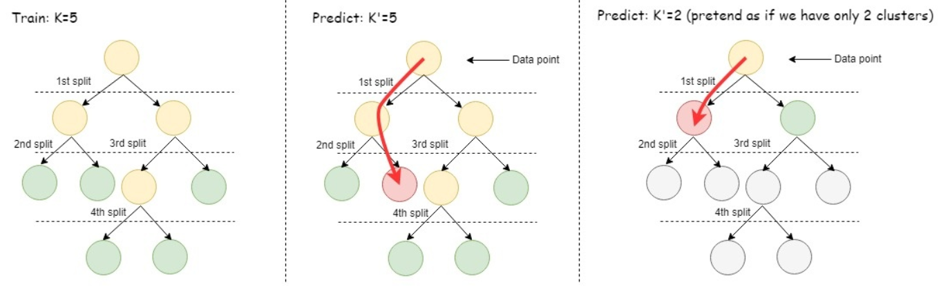
See also
6.6 - Time series forecasting
Time series models are trained on stationary time series (that is, time series where the mean doesn't change over time) of stochastic processes with consistent time steps.
Time series models are trained on stationary time series (that is, time series where the mean doesn't change over time) of stochastic processes with consistent time steps. These algorithms forecast future values by taking into account the influence of values at some number of preceding timesteps (lags).
Examples of applicable datasets include those for temperature, stock prices, earthquakes, product sales, etc.
To normalize datasets with inconsistent timesteps, see Gap filling and interpolation (GFI).
6.6.1 - Autoregressive model example
Autoregressive models predict future values of a time series based on the preceding values. More specifically, the user-specified lag determines how many previous timesteps it takes into account during computation, and predicted values are linear combinations of the values at each lag.
Use the following functions when training and predicting with autoregressive models. Note that these functions require datasets with consistent timesteps.
-
AUTOREGRESSOR: trains an autoregressive model -
PREDICT_AUTOREGRESSOR: applies the model to a dataset to make predictions
To normalize datasets with inconsistent timesteps, see Gap filling and interpolation (GFI).
Example
-
Load the datasets from the Machine-Learning-Examples repository.
This example uses the daily-min-temperatures dataset, which contains data on the daily minimum temperature in Melbourne, Australia from 1981 through 1990:
=> SELECT * FROM temp_data; time | Temperature ---------------------+------------- 1981-01-01 00:00:00 | 20.7 1981-01-02 00:00:00 | 17.9 1981-01-03 00:00:00 | 18.8 1981-01-04 00:00:00 | 14.6 1981-01-05 00:00:00 | 15.8 ... 1990-12-27 00:00:00 | 14 1990-12-28 00:00:00 | 13.6 1990-12-29 00:00:00 | 13.5 1990-12-30 00:00:00 | 15.7 1990-12-31 00:00:00 | 13 (3650 rows) -
Use
AUTOREGRESSORto create the autoregressive modelAR_temperaturefrom thetemp_datadataset. In this case, the model is trained with a lag ofp=3, taking the previous 3 entries into account for each estimation:=> SELECT AUTOREGRESSOR('AR_temperature', 'temp_data', 'Temperature', 'time' USING PARAMETERS p=3); AUTOREGRESSOR --------------------------------------------------------- Finished. 3650 elements accepted, 0 elements rejected. (1 row)You can view a summary of the model with
GET_MODEL_SUMMARY:=> SELECT GET_MODEL_SUMMARY(USING PARAMETERS model_name='AR_temperature'); GET_MODEL_SUMMARY ------------------- ============ coefficients ============ parameter| value ---------+-------- alpha | 1.88817 phi_(t-1)| 0.70004 phi_(t-2)|-0.05940 phi_(t-3)| 0.19018 ================== mean_squared_error ================== not evaluated =========== call_string =========== autoregressor('public.AR_temperature', 'temp_data', 'temperature', 'time' USING PARAMETERS p=3, missing=linear_interpolation, regularization='none', lambda=1, compute_mse=false); =============== Additional Info =============== Name |Value ------------------+----- lag_order | 3 rejected_row_count| 0 accepted_row_count|3650 (1 row) -
Use
PREDICT_AUTOREGRESSORto predict future temperatures. The following querystarts the prediction at the end of the dataset and returns 10 predictions.=> SELECT PREDICT_AUTOREGRESSOR(Temperature USING PARAMETERS model_name='AR_temperature', npredictions=10) OVER(ORDER BY time) FROM temp_data; prediction ------------------ 12.6235419917807 12.9387860506032 12.6683380680058 12.3886937385419 12.2689506237424 12.1503023330142 12.0211734746741 11.9150531529328 11.825870404008 11.7451846722395 (10 rows)
6.6.2 - Moving-average model example
Moving average models use the errors of previous predictions to make future predictions. More specifically, the user-specified lag determines how many previous predictions and errors it takes into account during computation.
Use the following functions when training and predicting with moving-average models. Note that these functions require datasets with consistent timesteps.
-
MOVING_AVERAGE: trains a moving-average model -
PREDICT_MOVING_AVERAGE: applies the model to a dataset to make predictions
To normalize datasets with inconsistent timesteps, see Gap filling and interpolation (GFI).
Example
-
Load the datasets from the Machine-Learning-Examples repository.
This example uses the daily-min-temperatures dataset, which contains data on the daily minimum temperature in Melbourne, Australia from 1981 through 1990:
=> SELECT * FROM temp_data; time | Temperature ---------------------+------------- 1981-01-01 00:00:00 | 20.7 1981-01-02 00:00:00 | 17.9 1981-01-03 00:00:00 | 18.8 1981-01-04 00:00:00 | 14.6 1981-01-05 00:00:00 | 15.8 ... 1990-12-27 00:00:00 | 14 1990-12-28 00:00:00 | 13.6 1990-12-29 00:00:00 | 13.5 1990-12-30 00:00:00 | 15.7 1990-12-31 00:00:00 | 13 (3650 rows) -
Use
MOVING_AVERAGEto create the moving-average modelMA_temperaturefrom thetemp_datadataset. In this case, the model is trained with a lag ofp=3, taking the error of 3 previous predictions into account for each estimation:=> SELECT MOVING_AVERAGE('MA_temperature', 'temp_data', 'temperature', 'time' USING PARAMETERS q=3, missing='linear_interpolation', regularization='none', lambda=1); MOVING_AVERAGE --------------------------------------------------------- Finished. 3650 elements accepted, 0 elements rejected. (1 row)You can view a summary of the model with
GET_MODEL_SUMMARY:=> SELECT GET_MODEL_SUMMARY(USING PARAMETERS model_name='MA_temperature'); GET_MODEL_SUMMARY ------------------- ============ coefficients ============ parameter| value ---------+-------- phi_(t-0)|-0.90051 phi_(t-1)|-0.10621 phi_(t-2)| 0.07173 =============== timeseries_name =============== temperature ============== timestamp_name ============== time =========== call_string =========== moving_average('public.MA_temperature', 'temp_data', 'temperature', 'time' USING PARAMETERS q=3, missing=linear_interpolation, regularization='none', lambda=1); =============== Additional Info =============== Name | Value ------------------+-------- mean |11.17780 lag_order | 3 lambda | 1.00000 rejected_row_count| 0 accepted_row_count| 3650 (1 row) -
Use
PREDICT_MOVING_AVERAGEto predict future temperatures. The following querystarts the prediction at the end of the dataset and returns 10 predictions.=> SELECT PREDICT_MOVING_AVERAGE(Temperature USING PARAMETERS model_name='MA_temperature', npredictions=10) OVER(ORDER BY time) FROM temp_data; prediction ------------------ 13.1324365636272 12.8071086272833 12.7218966671721 12.6011086656032 12.506624729879 12.4148247026733 12.3307873804812 12.2521385975133 12.1789741993396 12.1107640076638 (10 rows)
6.7 - Model management
The topics in this section describe how to manage models.
The topics in this section describe how to manage models.
6.7.1 - Altering models
You can modify a model using ALTER MODEL, in response to your model's needs.
You can modify a model using
ALTER MODEL, in response to your model's needs. You can alter a model by renaming the model, changing the owner, and changing the schema.
You can drop or alter any model that you create.
6.7.1.1 - Changing model ownership
As a superuser or model owner, you can reassign model ownership with ALTER MODEL as follows:.
As a superuser or model owner, you can reassign model ownership with
ALTER MODEL as follows:
ALTER MODEL model-nameOWNER TOowner-name
Changing model ownership is useful when a model owner leaves or changes responsibilities. Because you can change the owner, the models do not need to be rewritten.
Example
The following example shows how you can use ALTER_MODEL to change the model owner:
-
Find the model you want to alter. As the dbadmin, you own the model.
=> SELECT * FROM V_CATALOG.MODELS WHERE model_name='mykmeansmodel'; -[ RECORD 1 ]--+------------------------------------------ model_id | 45035996273816618 model_name | mykmeansmodel schema_id | 45035996273704978 schema_name | public owner_id | 45035996273704962 owner_name | dbadmin category | VERTICA_MODELS model_type | kmeans is_complete | t create_time | 2017-03-02 11:16:04.990626-05 size | 964 -
Change the model owner from dbadmin to user1.
=> ALTER MODEL mykmeansmodel OWNER TO user1; ALTER MODEL -
Review
V_CATALOG.MODELSto verify that the owner was changed.=> SELECT * FROM V_CATALOG.MODELS WHERE model_name='mykmeansmodel'; -[ RECORD 1 ]--+------------------------------------------ model_id | 45035996273816618 model_name | mykmeansmodel schema_id | 45035996273704978 schema_name | public owner_id | 45035996273704962 owner_name | user1 category | VERTICA_MODELS model_type | kmeans is_complete | t create_time | 2017-03-02 11:16:04.990626-05 size | 964
6.7.1.2 - Moving models to another schema
You can move a model from one schema to another with ALTER MODEL.
You can move a model from one schema to another with
ALTER MODEL. You can move the model as a superuser or user with USAGE privileges on the current schema and CREATE privileges on the destination schema.
Example
The following example shows how you can use ALTER MODEL to change the model schema:
-
Find the model you want to alter.
=> SELECT * FROM V_CATALOG.MODELS WHERE model_name='mykmeansmodel'; -[ RECORD 1 ]--+------------------------------------------ model_id | 45035996273816618 model_name | mykmeansmodel schema_id | 45035996273704978 schema_name | public owner_id | 45035996273704962 owner_name | dbadmin category | VERTICA_MODELS model_type | kmeans is_complete | t create_time | 2017-03-02 11:16:04.990626-05 size | 964 -
Change the model schema.
=> ALTER MODEL mykmeansmodel SET SCHEMA test; ALTER MODEL -
Review
V_CATALOG.MODELSto verify that the owner was changed.=> SELECT * FROM V_CATALOG.MODELS WHERE model_name='mykmeansmodel'; -[ RECORD 1 ]--+------------------------------------------ model_id | 45035996273816618 model_name | mykmeansmodel schema_id | 45035996273704978 schema_name | test owner_id | 45035996273704962 owner_name | dbadmin category | VERTICA_MODELS model_type | kmeans is_complete | t create_time | 2017-03-02 11:16:04.990626-05 size | 964
6.7.1.3 - Renaming a model
ALTER MODEL lets you rename models.
ALTER MODEL lets you rename models. For example:
-
Find the model you want to alter.
=> SELECT * FROM V_CATALOG.MODELS WHERE model_name='mymodel'; -[ RECORD 1 ]--+------------------------------------------ model_id | 45035996273816618 model_name | mymodel schema_id | 45035996273704978 schema_name | public owner_id | 45035996273704962 owner_name | dbadmin category | VERTICA_MODELS model_type | kmeans is_complete | t create_time | 2017-03-02 11:16:04.990626-05 size | 964 -
Rename the model.
=> ALTER MODEL mymodel RENAME TO mykmeansmodel; ALTER MODEL -
Review
V_CATALOG.MODELSto verify that the model name was changed.=> SELECT * FROM V_CATALOG.MODELS WHERE model_name='mykmeansmodel'; -[ RECORD 1 ]--+------------------------------------------ model_id | 45035996273816618 model_name | mykmeansmodel schema_id | 45035996273704978 schema_name | public owner_id | 45035996273704962 owner_name | dbadmin category | VERTICA_MODELS model_type | kmeans is_complete | t create_time | 2017-03-02 11:16:04.990626-05 size | 964
6.7.2 - Dropping models
DROP MODEL removes one or more models from the database.
DROP MODEL removes one or more models from the database. For example:
-
Find the model you want to drop.
=> SELECT * FROM V_CATALOG.MODELS WHERE model_name='mySvmClassModel'; -[ RECORD 1 ]--+-------------------------------- model_id | 45035996273765414 model_name | mySvmClassModel schema_id | 45035996273704978 schema_name | public owner_id | 45035996273704962 owner_name | dbadmin category | VERTICA_MODELS model_type | SVM_CLASSIFIER is_complete | t create_time | 2017-02-14 10:30:44.903946-05 size | 525 -
Drop the model.
=> DROP MODEL mySvmClassModel; DROP MODEL -
Review
V_CATALOG.MODELSto verify that the model was dropped.=> SELECT * FROM V_CATALOG.MODELS WHERE model_name='mySvmClassModel'; (0 rows)
6.7.3 - Managing model security
You can manage the security privileges on your models by using the GRANT and REVOKE statements.
You can manage the security privileges on your models by using the GRANT and REVOKE statements. The following examples show how you can change privileges on user1 and user2 using the faithful table and the linearReg model.
-
In the following example, the dbadmin grants the SELECT privilege to user1:
=> GRANT SELECT ON TABLE faithful TO user1; GRANT PRIVILEGE -
Then, the dbadmin grants the CREATE privilege on the public schema to user1:
=> GRANT CREATE ON SCHEMA public TO user1; GRANT PRIVILEGE -
Connect to the database as user1:
=> \c - user1 -
As user1, build the linearReg model:
=> SELECT LINEAR_REG('linearReg', 'faithful', 'waiting', 'eruptions');
LINEAR_REG
---------------------------
Finished in 1 iterations
(1 row)
- As user1, grant USAGE privileges to user2:
=> GRANT USAGE ON MODEL linearReg TO user2;
GRANT PRIVILEGE
- Connect to the database as user2:
=> \c - user2
- To confirm privileges were granted to user2, run the GET_MODEL_SUMMARY function. A user with the USAGE privilege on a model can run GET_MODEL_SUMMARY on that model:
=> SELECT GET_MODEL_SUMMARY(USING PARAMETERS model_name='linearReg');
=======
details
=======
predictor|coefficient|std_err |t_value |p_value
---------+-----------+--------+--------+--------
Intercept| 33.47440 | 1.15487|28.98533| 0.00000
eruptions| 10.72964 | 0.31475|34.08903| 0.00000
==============
regularization
==============
type| lambda
----+--------
none| 1.00000
===========
call_string
===========
linear_reg('public.linearReg', 'faithful', '"waiting"', 'eruptions'
USING PARAMETERS optimizer='newton', epsilon=1e-06, max_iterations=100, regularization='none', lambda=1)
===============
Additional Info
===============
Name |Value
------------------+-----
iteration_count | 1
rejected_row_count| 0
accepted_row_count| 272
(1 row)
- Connect to the database as user1:
=> \c - user1
- Then, you can use the REVOKE statement to revoke privileges from user2:
=> REVOKE USAGE ON MODEL linearReg FROM user2;
REVOKE PRIVILEGE
- To confirm the privileges were revoked, connect as user 2 and run the GET_MODEL_SUMMARY function:
=> \c - user2
=>SELECT GET_MODEL_SUMMARY('linearReg');
ERROR 7523: Problem in get_model_summary.
Detail: Permission denied for model linearReg
See also
6.7.4 - Viewing model attributes
The following topics explain the model attributes for the Vertica machine learning algorithms.
The following topics explain the model attributes for the Vertica machine learning algorithms. These attributes describe the internal structure of a particular model:
6.7.5 - Summarizing models
-
Find the model you want to summarize.
=> SELECT * FROM v_catalog.models WHERE model_name='svm_class'; model_id | model_name | schema_id | schema_name | owner_id | owner_name | category | model_type | is_complete | create_time | size -------------------+------------+-------------------+-------------+-------------------+------------+-------- --------+----------------+-------------+-------------------------------+------ 45035996273715226 | svm_class | 45035996273704980 | public | 45035996273704962 | dbadmin | VERTICA_MODELS | SVM_CLASSIFIER | t | 2017-08-28 09:49:00.082166-04 | 1427 (1 row) -
View the model summary.
=> SELECT GET_MODEL_SUMMARY(USING PARAMETERS model_name='svm_class'); ------------------------------------------------------------------------ ======= details ======= predictor|coefficient ---------+----------- Intercept| -0.02006 cyl | 0.15367 mpg | 0.15698 wt | -1.78157 hp | 0.00957 =========== call_string =========== SELECT svm_classifier('public.svm_class', 'mtcars_train', '"am"', 'cyl, mpg, wt, hp, gear' USING PARAMETERS exclude_columns='gear', C=1, max_iterations=100, epsilon=0.001); =============== Additional Info =============== Name |Value ------------------+----- accepted_row_count| 20 rejected_row_count| 0 iteration_count | 12 (1 row)
See also
6.7.6 - Viewing models
Vertica stores the models you create in the V_CATALOG.MODELS system table.
Vertica stores the models you create in the V_CATALOG.MODELS system table.
You can query V_CATALOG.MODELS to view information about the models you have created:
=> SELECT * FROM V_CATALOG.MODELS;
-[ RECORD 1 ]--+------------------------------------------
model_id | 45035996273765414
model_name | mySvmClassModel
schema_id | 45035996273704978
schema_name | public
owner_id | 45035996273704962
owner_name | dbadmin
category | VERTICA_MODELS
model_type | SVM_CLASSIFIER
is_complete | t
create_time | 2017-02-14 10:30:44.903946-05
size | 525
-[ RECORD 2 ]--+------------------------------------------
model_id | 45035996273711466
model_name | mtcars_normfit
schema_id | 45035996273704978
schema_name | public
owner_id | 45035996273704962
owner_name | dbadmin
category | VERTICA_MODELS
model_type | SVM_CLASSIFIER
is_complete | t
create_time | 2017-02-06 15:03:05.651941-05
size | 288
See also
6.8 - Using external models with Vertica
To give you the utmost in machine learning flexibility and scalability, Vertica supports importing, exporting, and predicting with PMML and TensorFlow models.
To give you the utmost in machine learning flexibility and scalability, Vertica supports importing, exporting, and predicting with PMML and TensorFlow models.
The machine learning configuration parameter MaxModelSizeKB sets the maximum size of a model that can be imported into Vertica.
Support for PMML models
Vertica supports the import and export of K-means, linear regression, and logistic regression machine learning models in Predictive Model Markup Language (PMML) format. Support for this platform-independent model format allows you to use models trained on other platforms to predict on data stored in your Vertica database. You can also use Vertica as your model repository. Vertica supports PMML version 4.4.
With the PREDICT_PMML function, you can use a PMML model archived in Vertica to run prediction on data stored in the Vertica database.
For more information, see Using PMML models.
For details on the PMML attributes that Vertica does and does not currently support, see PMML features and attributes.
Support for TensorFlow models
Vertica now supports importing trained TensorFlow models, and using those models to do prediction in Vertica on data stored in the Vertica database. Vertica supports TensorFlow models trained in TensorFlow version 1.15.
The PREDICT_TENSORFLOW function lets you predict on data in Vertica with any TensorFlow model.
For additional information, see TensorFlow models.
Additional functions that support external models
The following functions support both PMML and TensorFlow models:
IMPORT_MODELS EXPORT_MODELS GET_MODEL_ATTRIBUTE GET_MODEL_SUMMARY6.8.1 - TensorFlow models
Tensorflow is a framework for creating neural networks.
Tensorflow is a framework for creating neural networks. It implements basic linear algebra and multi-variable calculus operations in a scalable fashion, and allows users to easily chain these operations into a computation graph.
Vertica supports importing, exporting, and making predictions with TensorFlow 1.x and 2.x models trained outside of Vertica.
In-database TensorFlow integration with Vertica offers several advantages:
-
Your models live inside your database, so you never have to move your data to make predictions.
-
The volume of data you can handle is limited only by the size of your Vertica database, which makes Vertica particularly well-suited for machine learning on Big Data.
-
Vertica offers in-database model management, so you can store as many models as you want.
-
Imported models are portable and can be exported for use elsewhere.
When you run a TensorFlow model to predict on data in the database, Vertica calls a TensorFlow process to run the model. This allows Vertica to support any model you can create and train using TensorFlow. Vertica just provides the inputs - your data in the Vertica database - and stores the outputs.
6.8.1.1 - TensorFlow integration and directory structure
This page covers importing Tensorflow models into Vertica, making predictions on data in the Vertica database, and exporting the model for use on another Vertica cluster or a third-party platform.
This page covers importing Tensorflow models into Vertica, making predictions on data in the Vertica database, and exporting the model for use on another Vertica cluster or a third-party platform.
For a start-to-finish example through each operation, see TensorFlow example.
Vertica supports models created with either TensorFlow 1.x and 2.x, but 2.x is strongly recommended.
To use TensorFlow with Vertica, install the TFIntegration UDX package on any node. You only need to do this once:
$ /opt/vertica/bin/admintools -t install_package -d database_name -p 'password' --package TFIntegration
Directory and file structure for TensorFlow models
Before importing your models, you should have a separate directory for each model that contains one of each of the following. Note that Vertica uses the directory name as the model name when you import it:
-
model_name.pb: a trained model in frozen graph format -
tf_model_desc.json: a description of the model
You can generate both files for a given TensorFlow 2 model with the script freeze_tf2_model.py included in Machine-Learning-Examples/TensorFlow repository (or in opt/vertica/packages/TFIntegration/examples), though you may need to make modifications to the description based on your use-case and how you want your Vertica database to interact with your model:
$ python3 Tensorflow/freeze_tf2_model.py your/model/directory
For example, the tf_models directory contains two models, tf_mnist_estimator and tf_mnist_keras:
tf_models/
├── tf_mnist_estimator
│ ├── mnist_estimator.pb
│ └── tf_model_desc.json
└── tf_mnist_keras
├── mnist_keras.pb
└── tf_model_desc.json
tf_model_desc.json
The tf_model_desc.json file forms the bridge between TensorFlow and Vertica. It describes the structure of the model so that Vertica can correctly match up its inputs and outputs to input/output tables.
Notice that the freeze_tf2_model.py script automatically generates this file for your model, and this generated file can often be used as-is. For more complex models or use cases, you might have to edit this file. For a detailed breakdown of each field, see tf_model_desc.json overview.
Importing TensorFlow models into Vertica
To import TensorFlow models, use IMPORT_MODELS with the category 'TENSORFLOW'.
Import a single model. Keep in mind that the Vertica database uses the directory name as the model name:
select IMPORT_MODELS ( '/path/tf_models/tf_mnist_keras' USING PARAMETERS category='TENSORFLOW');
import_models
---------------
Success
(1 row)
Import all models in the directory (where each model has its own directory) with a wildcard (*):
select IMPORT_MODELS ('/path/tf_models/*' USING PARAMETERS category='TENSORFLOW');
import_models
---------------
Success
(1 row)
Predicting with an imported TensorFlow model
After importing your TensorFlow model, you can use the model to predict on data in a Vertica table.
The PREDICT_TENSORFLOW function is different from the other predict functions in that it does not accept any parameters that affect the input columns such as "exclude_columns" or "id_column"; rather, the function always predicts on all the input columns provided. However, it does accept a num_passthru_cols parameter which allows the user to "skip" some number of input columns, as shown below.
The OVER(PARTITION BEST) clause tells Vertica to parallelize the operation across multiple nodes. See Window partition clause for details:
=> select PREDICT_TENSORFLOW (*
USING PARAMETERS model_name='tf_mnist_keras', num_passthru_cols=1)
OVER(PARTITION BEST) FROM tf_mnist_test_images;
--example output, the skipped columns are displayed as the first columns of the output
ID | col0 | col1 | col2 | col3 | col4 | col5 | col6 | col7 | col8 | col9
----+------+------+------+------+------+------+------+------+------+------
1 | 0 | 0 | 1 | 0 | 0 | 0 | 0 | 0 | 0 | 0
3 | 1 | 0 | 0 | 0 | 0 | 0 | 0 | 0 | 0 | 0
6 | 0 | 0 | 0 | 0 | 1 | 0 | 0 | 0 | 0 | 0
...
Exporting TensorFlow models
Vertica exports the model as a frozen graph, which can then be re-imported at any time. Keep in mind that models that are saved as a frozen graph cannot be trained further.
Use EXPORT_MODELS to export TensorFlow models. For example, to export the tf_mnist_keras model to the /path/to/export/to directory:
=> SELECT EXPORT_MODELS ('/path/to/export/to', 'tf_mnist_keras');
export_models
---------------
Success
(1 row)
When you export a TensorFlow model, the Vertica database creates and uses the specified directory to store files that describe the model:
$ ls tf_mnist_keras/
crc.json metadata.json mnist_keras.pb model.json tf_model_desc.json
The .pb and tf_model_desc.json files describe the model, and the rest are organizational files created by the Vertica database.
| File Name | Purpose |
|---|---|
model_name.pb |
Frozen graph of the model. |
tf_model_desc.json |
Describes the model. |
crc.json |
Keeps track of files in this directory and their sizes. It is used for importing models. |
metadata.json |
Contains Vertica version, model type, and other information. |
model.json |
More verbose version of tf_model_desc.json. |
See also
6.8.1.2 - TensorFlow example
Vertica uses the TFIntegration UDX package to integrate with TensorFlow.
Vertica uses the TFIntegration UDX package to integrate with TensorFlow. You can train your models outside of your Vertica database, then import them to Vertica and make predictions on your data.
TensorFlow scripts and datasets are included in the GitHub repository under Machine-Learning-Examples/TensorFlow.
The example below creates a Keras (a TensorFlow API) neural network model trained on the MNIST handwritten digit classification dataset, the layers of which are shown below.
The data is fed through each layer from top to bottom, and each layer modifies the input before returning a score. In this example, the data passed in is a set of images of handwritten Arabic numerals and the output would be the probability of the input image being a particular digit:
inputs = keras.Input(shape=(28, 28, 1), name="image")
x = layers.Conv2D(32, 5, activation="relu")(inputs)
x = layers.MaxPooling2D(2)(x)
x = layers.Conv2D(64, 5, activation="relu")(x)
x = layers.MaxPooling2D(2)(x)
x = layers.Flatten()(x)
x = layers.Dense(10, activation='softmax', name='OUTPUT')(x)
tfmodel = keras.Model(inputs, x)
For more information on how TensorFlow interacts with your Vertica database and how to import more complex models, see TensorFlow integration and directory structure.
Prepare a TensorFlow model for Vertica
The following procedures take place outside of Vertica.
Train and save a TensorFlow model
-
Train your model. For this particular example, you can run train_simple_model.py to train and save the model. Otherwise, and more generally, you can manually train your model in Python and then save it:
$ mymodel.save('my_saved_model_dir') -
Run the
freeze_tf2_model.pyscript included in the Machine-Learning-Examples repository or inopt/vertica/packages/TFIntegration/examples, specifying your model and an output directory (optional, defaults tofrozen_tfmodel).This script transforms your saved model into the Vertica-compatible frozen graph format and creates the
tf_model_desc.jsonfile, which describes how Vertica should translate its tables to TensorFlow tensors:$ ./freeze_tf2_model.py path/to/tf/model frozen_model_dir
Import TensorFlow models and make predictions in Vertica
-
If you haven't already, as
dbadmin, install the TFIntegration UDX package on any node. You only need to do this once.$ /opt/vertica/bin/admintools -t install_package -d database_name -p 'password' --package TFIntegration -
Copy the the
directoryto any node in your Vertica cluster and import the model:=> SELECT IMPORT_MODELS('path/to/frozen_model_dir' USING PARAMETERS category='TENSORFLOW'); -
Import the dataset you want to make a prediction on. For this example:
-
Copy the
Machine-Learning-Examples/TensorFlow/datadirectory to any node on your Vertica cluster. -
From that
datadirectory, run the SQL scriptload_tf_data.sqlto load the MNIST dataset:$ vsql -f load_tf_data.sql
-
-
Make a prediction with your model on your dataset with PREDICT_TENSORFLOW. In this example, the model is used to classify the images of handwritten numbers in the MNIST dataset:
=> SELECT PREDICT_TENSORFLOW (* USING PARAMETERS model_name='tf_mnist_keras', num_passthru_cols=1) OVER(PARTITION BEST) FROM tf_mnist_test_images; --example output, the skipped columns are displayed as the first columns of the output ID | col0 | col1 | col2 | col3 | col4 | col5 | col6 | col7 | col8 | col9 ----+------+------+------+------+------+------+------+------+------+------ 1 | 0 | 0 | 1 | 0 | 0 | 0 | 0 | 0 | 0 | 0 3 | 1 | 0 | 0 | 0 | 0 | 0 | 0 | 0 | 0 | 0 6 | 0 | 0 | 0 | 0 | 1 | 0 | 0 | 0 | 0 | 0 ... -
To export the model with EXPORT_MODELS:
=> SELECT EXPORT_MODELS('/path/to/export/to', 'tf_mnist_keras'); EXPORT_MODELS --------------- Success (1 row)
Note
While you cannot continue training a TensorFlow model after you export it from Vertica, you can use it to predict on data in another Vertica cluster, or outside Vertica on another platform.TensorFlow 1 (deprecated)
-
Install TensorFlow 1.15 with Python 3.7 or below.
-
Run
train_save_model.pyinMachine-Learning-Examples/TensorFlow/tf1to train and save the model in TensorFlow and frozen graph formats.
See also
6.8.1.3 - tf_model_desc.json overview
Before importing your externally trained TensorFlow models, you must:.
Before importing your externally trained TensorFlow models, you must:
-
save the model in frozen graph (
.pb) format -
create
tf_model_desc.json, which describes to your Vertica database how to map its inputs and outputs to input/output tables
Conveniently, the script freeze_tf2_model.py included in the TensorFlow directory of the Machine-Learning-Examples repository (and in opt/vertica/packages/TFIntegration/examples) will do both of these automatically. In most cases, the generated tf_model_desc.json can be used as-is, but for more complex datasets and use cases, you might need to edit it.
tf_model_desc.json for an example dataset
The following tf_model_desc.json is generated from the MNIST handwriting dataset used by the TensorFlow example.
{
"frozen_graph": "mnist_keras.pb",
"input_desc": [
{
"op_name": "image_input",
"tensor_map": [
{
"idx": 0,
"dim": [
1,
28,
28,
1
],
"col_start": 0
}
]
}
],
"output_desc": [
{
"op_name": "OUTPUT/Softmax",
"tensor_map": [
{
"idx": 0,
"dim": [
1,
10
],
"col_start": 0
}
]
}
]
}
This file describes the structure of the model's inputs and outputs. It must contain a frozen_graph field that matches the filename of the .pb model, an input_desc field, and an output_desc field.
- input_desc and output_desc: the descriptions of the input and output nodes in the TensorFlow graph. Each of these include the following fields:
-
op_name: the name of the operation node which is set when creating and training the model. You can typically retrieve the names of these parameters from
tfmodel.inputsandtfmodel.outputs. For example:$ print({t.name:t for t in tfmodel.inputs}) {'image_input:0': <tf.Tensor 'image_input:0' shape=(?, 28, 28, 1) dtype=float32>}$ print({t.name:t for t in tfmodel.outputs}) {'OUTPUT/Softmax:0': <tf.Tensor 'OUTPUT/Softmax:0' shape=(?, 10) dtype=float32>}In this case, the respective values for op_name would be the following.
-
input_desc:image_input -
output_desc:OUTPUT/Softmax
For a more detailed example of this process, review the code for
freeze_tf2_model.py. -
-
tensor_map: how to map the tensor to Vertica columns, which can be specified with the following:
-
idx: the index of the tensor (should be 0 for the first input/output, 1 for the second input/output, etc.)
-
dim: the vector holding the dimensions of the tensor; it provides the number of columns
-
col_start (only used if col_idx is not specified): the starting column index. When used with dim, it specifies a range of indices of Vertica columns starting at col_start and ending at col_start+dim; Vertica starts at the column specified by the index col_start and gets the next dim columns
-
col_idx: the indices in the Vertica columns corresponding to the flattened tensors. This allows you explicitly specify the indices of the Vertica columns that couldn't otherwise be specified as a simple range with col_start and dim (e.g. 1, 3, 5, 7)
-
data_type (not shown): the data type of the input or output, one of the following:
-
TF_FLOAT (default)
-
TF_DOUBLE
-
TF_INT8
-
TF_INT16
-
TF_INT32
-
TF_INT64
-
-
-
Complex tf_model_desc.json example
Below is a more complex example that includes multiple inputs and outputs:
{
"input_desc": [
{
"op_name": "input1",
"tensor_map": [
{
"idx": 0,
"dim": [
4
],
"col_idx": [
0,
1,
2,
3
]
},
{
"idx": 1,
"dim": [
2,
2
],
"col_start": 4
}
]
},
{
"op_name": "input2",
"tensor_map": [
{
"idx": 0,
"dim": [],
"col_idx": [
8
]
},
{
"idx": 1,
"dim": [
2
],
"col_start": 9
}
]
}
],
"output_desc": [
{
"op_name": "output",
"tensor_map": [
{
"idx": 0,
"dim": [
2
],
"col_start": 0
}
]
}
]
}
See also
6.8.2 - Using PMML models
Vertica can import, export, and make predictions with PMML models of version 4.4 and below.
Vertica can import, export, and make predictions with PMML models of version 4.4 and below.
6.8.2.1 - Exporting Vertica models in PMML format
You can take advantage of the built-in distributed algorithms in Vertica to train machine learning models.
You can take advantage of the built-in distributed algorithms in Vertica to train machine learning models. There might be cases in which you want to use these models for prediction outside Vertica, for example on an edge node. Now, you can export your model in PMML format and use it for prediction using a library or platform that supports reading and evaluating PMML models.
Here is an example for training a model in Vertica and then exporting it in PMML format. The following diagram shows the workflow of the example. We use vsql to run this example.
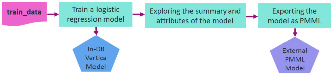
Let's assume that you want to train a logistic regression model on the data in a relation named 'patients' in order to predict the second attack of patients given their treatment and trait anxiety.
After training, the model is shown in a system table named V_CATALOG.MODELS which lists the archived ML models in Vertica.
=> -- Training a logistic regression model on a training_data
=> SELECT logistic_reg('myModel', 'patients', 'second_attack', 'treatment, trait_anxiety');
logistic_reg
---------------------------
Finished in 5 iterations
(1 row)
=> -- Looking at the models table
=> SELECT model_name, schema_name, category, model_type, create_time, size FROM models;
model_name | schema_name | category | model_type | create_time | size
------------+-------------+----------------+---------------------+-------------------------------+------
myModel | public | VERTICA_MODELS | LOGISTIC_REGRESSION | 2020-07-28 00:05:18.441958-04 | 1845
(1 row)
You can look at the summary of the model using the GET_MODEL_SUMMARY function.
=> -- Looking at the summary of the model
=> \t
Showing only tuples.
=> SELECT get_model_summary(USING PARAMETERS model_name='myModel');
=======
details
=======
predictor |coefficient|std_err |z_value |p_value
-------------+-----------+--------+--------+--------
Intercept | -6.36347 | 3.21390|-1.97998| 0.04771
treatment | -1.02411 | 1.17108|-0.87450| 0.38185
trait_anxiety| 0.11904 | 0.05498| 2.16527| 0.03037
==============
regularization
==============
type| lambda
----+--------
none| 1.00000
===========
call_string
===========
logistic_reg('public.myModel', 'patients', '"second_attack"', 'treatment, trait_anxiety'
USING PARAMETERS optimizer='newton', epsilon=1e-06, max_iterations=100, regularization='none', lambda=1, alpha=0.5)
===============
Additional Info
===============
Name |Value
------------------+-----
iteration_count | 5
rejected_row_count| 0
accepted_row_count| 20
You can also retrieve the model's attributes using the GET_MODEL_ATTRIBUTE function.
=> \t
Tuples only is off.
=> -- The list of the attributes of the model
=> SELECT get_model_attribute(USING PARAMETERS model_name='myModel');
attr_name | attr_fields | #_of_rows
--------------------+---------------------------------------------------+-----------
details | predictor, coefficient, std_err, z_value, p_value | 3
regularization | type, lambda | 1
iteration_count | iteration_count | 1
rejected_row_count | rejected_row_count | 1
accepted_row_count | accepted_row_count | 1
call_string | call_string | 1
(6 rows)
=> -- Returning the coefficients of the model in a tabular format
=> SELECT get_model_attribute(USING PARAMETERS model_name='myModel', attr_name='details');
predictor | coefficient | std_err | z_value | p_value
---------------+-------------------+--------------------+--------------------+--------------------
Intercept | -6.36346994178182 | 3.21390452471434 | -1.97998101463435 | 0.0477056620380991
treatment | -1.02410605239327 | 1.1710801464903 | -0.874496980810833 | 0.381847663704613
trait_anxiety | 0.119044916668605 | 0.0549791755747139 | 2.16527285875412 | 0.0303667955962211
(3 rows)
You can use the EXPORT_MODELS function in a simple statement to export the model in PMML format, as shown below.
=> -- Exporting the model as PMML
=> SELECT export_models('/data/username/temp', 'myModel' USING PARAMETERS category='PMML');
export_models
---------------
Success
(1 row)
See also
6.8.2.2 - Importing and predicting with PMML models
As a Vertica user, you can train ML models in other platforms, convert them to standard PMML format, and then import them into Vertica for in-database prediction on data stored in Vertica relations.
As a Vertica user, you can train ML models in other platforms, convert them to standard PMML format, and then import them into Vertica for in-database prediction on data stored in Vertica relations.
Here is an example of how to import a PMML model trained in Spark. The following diagram shows the workflow of the example.
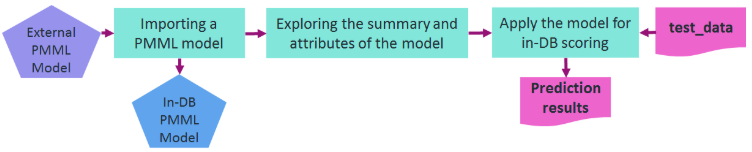
You can use the IMPORT_MODELS function in a simple statement to import the PMML model. The imported model then appears in a system table named V_CATALOG.MODELS which lists the archived ML models in Vertica.
=> -- importing the PMML model trained and generated in Spark
=> SELECT import_models('/data/username/temp/spark_logistic_reg' USING PARAMETERS category='PMML');
import_models
---------------
Success
(1 row)
=> -- Looking at the models table=> SELECT model_name, schema_name, category, model_type, create_time, size FROM models;
model_name | schema_name | category | model_type | create_time | size
--------------------+-------------+----------+-----------------------+-------------------------------+------
spark_logistic_reg | public | PMML | PMML_REGRESSION_MODEL | 2020-07-28 00:12:29.389709-04 | 5831
(1 row)
You can look at the summary of the model using GET_MODEL_SUMMARY function.
=> \t
Showing only tuples.
=> SELECT get_model_summary(USING PARAMETERS model_name='spark_logistic_reg');
=============
function_name
=============
classification
===========
data_fields
===========
name |dataType| optype
-------+--------+-----------
field_0| double |continuous
field_1| double |continuous
field_2| double |continuous
field_3| double |continuous
field_4| double |continuous
field_5| double |continuous
field_6| double |continuous
field_7| double |continuous
field_8| double |continuous
target | string |categorical
==========
predictors
==========
name |exponent|coefficient
-------+--------+-----------
field_0| 1 | -0.23318
field_1| 1 | 0.73623
field_2| 1 | 0.29964
field_3| 1 | 0.12809
field_4| 1 | -0.66857
field_5| 1 | 0.51675
field_6| 1 | -0.41026
field_7| 1 | 0.30829
field_8| 1 | -0.17788
===============
Additional Info
===============
Name | Value
-------------+--------
is_supervised| 1
intercept |-1.20173
You can also retrieve the model's attributes using the GET_MODEL_ATTRIBUTE function.
=> \t
Tuples only is off.
=> -- The list of the attributes of the PMML model
=> SELECT get_model_attribute(USING PARAMETERS model_name='spark_logistic_reg');
attr_name | attr_fields | #_of_rows
---------------+-----------------------------+-----------
is_supervised | is_supervised | 1
function_name | function_name | 1
data_fields | name, dataType, optype | 10
intercept | intercept | 1
predictors | name, exponent, coefficient | 9
(5 rows)
=> -- The coefficients of the PMML model
=> SELECT get_model_attribute(USING PARAMETERS model_name='spark_logistic_reg', attr_name='predictors');
name | exponent | coefficient
---------+----------+--------------------
field_0 | 1 | -0.2331769167607
field_1 | 1 | 0.736227459496199
field_2 | 1 | 0.29963728232024
field_3 | 1 | 0.128085369856188
field_4 | 1 | -0.668573096260048
field_5 | 1 | 0.516750679584637
field_6 | 1 | -0.41025989394959
field_7 | 1 | 0.308289533913736
field_8 | 1 | -0.177878773139411
(9 rows)
You can then use the PREDICT_PMML function to apply the imported model on a relation for in-database prediction. The internal parameters of the model can be matched to the column names of the input relation by their names or their listed position. Direct input values can also be fed to the function as displayed below.
=> -- Using the imported PMML model for scoring direct input values
=> SELECT predict_pmml(1.5,0.5,2,1,0.75,4.2,3.1,0.9,1.1
username(> USING PARAMETERS model_name='spark_logistic_reg', match_by_pos=true);
predict_pmml
--------------
1
(1 row)
=> -- Using the imported PMML model for scoring samples in a table
=> SELECT predict_pmml(* USING PARAMETERS model_name='spark_logistic_reg') AS prediction
=> FROM test_data;
prediction
------------
1
0
(2 rows)
See also
6.8.2.3 - PMML features and attributes
Using External Models With Vertica gives an overview of the features Vertica supports for working with external models.
Using external models with Vertica gives an overview of the features Vertica supports for working with external models. This topic provides additional details on limitations in how Vertica supports working with PMML models.
In order to be supported by Vertica, PMML models:
-
Must not contain a data preprocessing step.
-
Must encode only these model types: k-means, linear regression, logistic regression, random forest (classifier and regressor), XGBoost (classifier and regressor), GeneralRegressionModel, and TreeModel.
Supported PMML tags and attributes
The following table lists supported PMML tags and their attributes.
| XML-tag name | Ignored attributes | Supported attributes | Unsupported attributes | Ignored sub-tags | Supported sub-tags | Unsupported sub-tags |
|---|---|---|---|---|---|---|
| Categories | - |
|
- | - | Category | Extension |
| Category | - | value (required) | - | - | - | Extension |
| CategoricalPredictor | - |
|
- | - | - | Extension |
| Cluster | size |
|
- |
|
NUM-ARRAY |
|
| ClusteringField | - |
|
|
- | - |
|
| ClusteringModel | modelName |
|
- | ModelVerification |
|
|
| ComparisonMeasure |
|
|
- | - |
|
|
| CompoundPredicate | - | booleanOperator (required) | - | - | Extension | |
| CovariateList | - | - | - | - | Predictor | Extension |
| DataDictionary | - | numberOfFields | - | - | DataField |
|
| DataField | displayName |
|
|
- | Value |
|
| FactorList | - | - | - | - | Predictor | Extension |
| False | - | - | - | - | - | Extension |
| GeneralRegressionModel |
|
|
|
|
|
|
| Header |
|
- | - |
|
- | - |
| MiningField |
|
|
|
- | - | Extension |
| MiningModel |
|
|
- | ModelVerification | ||
| MiningSchema | - | - | - | - | MiningField | Extension |
| Node | - |
|
- | - | ||
| NumericPredictor | - |
|
- | - | - | Extension |
| Output | - | - | - | - | OutputField | Extension |
| OutputField |
|
|
|
- | - |
|
| Parameter | - |
|
referencePoint | - | - | Extension |
| ParameterList | - | - | - | - | Parameter | Extension |
| ParamMatrix | - | - | - | - | PCell | Extension |
| PCell | - |
|
- | - | - | Extension |
| PPCell | - |
|
- | - | - | Extension |
| PPMatrix | - | - | - | - | PPCell | Extension |
| PMML | - |
|
- | MiningBuildTask |
|
|
| Predictor | - |
|
- | - | Extension | |
| RegressionModel |
|
|
- | ModelVerification |
|
|
| RegressionTable | - |
|
- | - |
|
|
| Segment | - |
|
|
- | ||
| Segmentation |
|
multipleModelMethod (required) | - | - | Segment | Extension |
| SimplePredicate | - |
|
- | - | - | Extension |
| SimpleSetPredicate | - |
|
- | - | ARRAY | Extension |
| Target | - |
|
|
- | - | |
| Targets | - | - | - | - | Target | Extension |
| TreeModel |
|
|
- | ModelVerification | ||
| True | - | - | - | - | - | Extension |
| ScoreDistribution | - |
|
- | - | - | Extension |
| Value | displayValue |
|
- | - | - | Extension |
7 - Geospatial analytics
Vertica provides functions that allows you to manipulate complex two- and three-dimensional spatial objects.
Vertica provides functions that allows you to manipulate complex two- and three-dimensional spatial objects. These functions follow the Open Geospatial Consortium (OGC) standards. Vertica also provides data types and SQL functions that allow you to specify and store spatial objects in a database according to OGC standards.
Convert well-known text (WKT) and well-known binary (WKB)
Convert WKT and WKB.
Optimized spatial joins
Perform fast spatial joins using ST_Intersects and STV_Intersects.
Load and export spatial data from shapefiles
Easily load and export shapefiles.
Store and retrieve objects
Determine if:
-
An object contains self-intersection or self-tangency points.
-
One object is entirely within another object, such as a point within a polygon.
Test the relationships between objects
For example, if they intersect or touch:
-
Identify the boundary of an object.
-
Identify vertices of an object.
Calculate
-
Shortest distance between two objects.
-
Size of an object (length, area).
-
Centroid for one or more objects.
-
Buffer around one or more objects.
7.1 - Best practices for geospatial analytics
Vertica recommends the following best practices when performing geospatial analytics in Vertica.
Vertica recommends the following best practices when performing geospatial analytics in Vertica.
Performance optimization
| Recommendation | Details |
|---|---|
| Use the minimum column size for spatial data. | Performance degrades as column widths increase. When creating columns for your spatial data, use the smallest size column that can accommodate your data. For example, use GEOMETRY(85) for point data. |
| Use GEOMETRY types where possible. | Performance of functions on GEOGRAPHY types is slower than functions that support GEOMETRY types. Use GEOMETRY types where possible. |
|
To improve the performance of the following functions, sort projections on spatial columns:
|
You may improve the pruning efficiency of these functions by sorting the projection on the GEOMETRY column. However, sorting on a large GEOMETRY column may slow down data load. |
Spatial joins with points and polygons
Vertica provides two ways to identify whether a set of points intersect with a set of polygons. Depending on the size of your data set, choose the approach that gives the best performance.
For a detailed example of best practices with spatial joins, see Best practices for spatial joins.
| Recommendation | Details |
|---|---|
| Use ST_Intersects to intersect a constant geometry with a set of geometries. |
When you intersect a set of geometries with a geometry, use the ST_Intersects function. Express the constant geometry argument as a WKT or WKB. For example:
For more information, see Performing spatial joins with ST_Intersects. |
| Create a spatial index only when performing spatial joins with STV_Intersect. | Spatial indexes should only be used with STV_Intersect. Creating a spatial index and then performing spatial joins with ST_Intersects will not improve performance. |
| Use the STV_Intersect function when you intersect a set of points with a set of polygons. |
Determine if a set of points intersects with a set of polygons in a medium to large data set. First, create a spatial index using STV_Create_Index. Then, use one of the STV_Intersect functions to return the set of pairs that intersect. Spatial indexes provide the best performance for accessing a large number of polygons. |
| When using the STV_Intersect transform function, partition the data and use an OVER(PARTITION BEST) clause. | The STV_Intersect transform function does not require that you partition the data. However, you may improve performance by partitioning the data and using an OVER(PARTITION BEST) clause. |
Spatial indexes
The STV_Create_Index function can consume large amounts of processing time and memory. When you index new data for the first time, monitor memory usage to be sure it stays within safe limits. Memory usage depends on:
-
Number of polygons
-
Number of vertices
-
Amount of overlap among polygons
| Recommendation | Details |
|---|---|
| Segment polygon data when a table contains a large number of polygons. | Segmenting the data allows the index creation process to run in parallel. This is advantageous because sometimes STV_Create_Index tasks cannot be completed when large tables that are not segmented prior to index creation. |
| Adjust STV_Create_Index parameters as needed for memory allocation and CPU usage. |
The Default: 256 Valid values: Any value less than or equal to the amount of memory in the GENERAL resource pool. Assigning a higher value results in an error. |
| Make changes if STV_Create_Index cannot allocate 300 MB memory. |
Before STV_Create_Index starts creating the index, it tries to allocate about 300 MB of memory. If that much memory is not available, the function fails. If you get a failure message, try these solutions:
|
| Create misplaced indexes again, if needed. | When you back up your Vertica database, spatial index files are not included. If you misplace an index, use STV_Create_Index to re-create it. |
| Use STV_Refresh_Index to add new or updated polygons to an existing index. | Instead of rebuilding your spatial index each time you add new or updated polygons to a table, you can use STV_Refresh_Index to append the polygons to your existing spatial index. |
Checking polygon validity
| Recommendation | Details |
|---|---|
| Run ST_IsValid to check if polygons are valid. |
Many spatial functions do not check the validity of polygons.
For more information, see Ensuring polygon validity before creating or refreshing an index. |
7.2 - Spatial objects
Vertica implements several data types for storing spatial objects, Well-Known Text (WKT) strings, and Well-Known Binary (WKB) representations.
Vertica implements several data types for storing spatial objects, Well-Known Text (WKT) strings, and Well-Known Binary (WKB) representations. These data types include:
7.2.1 - Supported spatial objects
Vertica supports two spatial data types. These data types store two- and three-dimensional spatial objects in a table column:
GEOMETRY: Spatial object with coordinates expressed as (x,y) pairs, defined in the Cartesian plane. All calculations use Cartesian coordinates.GEOGRAPHY: Spatial object defined as on the surface of a perfect sphere, or a spatial object in the WGS84 coordinate system. Coordinates are expressed in longitude/latitude angular values, measured in degrees. All calculations are in meters. For perfect sphere calculations, the sphere has a radius of 6371 kilometers, which approximates the shape of the earth.Note
Some spatial programs use an ellipsoid to model the earth, resulting in slightly different data.
The maximum size of a GEOMETRY or GEOGRAPHY data type is 10,000,000 bytes (10 MB). You cannot use either data type as a table's primary key.
7.2.2 - Spatial reference identifiers (SRIDs)
A spatial reference identifier (SRID) is an integer value that represents a method for projecting coordinates on the plane.
A spatial reference identifier (SRID) is an integer value that represents a method for projecting coordinates on the plane. A SRID is metadata that indicates the coordinate system in which a spatial object is defined.
Geospatial functions using Geometry arguments must contain the same SRID. If the functions do not contain the same SRID, then the query returns an error.
For example, in this query the two points have different SRIDs. As a result the query returns an error:
=> SELECT ST_Distance(ST_GeomFromText('POINT(34 9)',2749), ST_GeomFromText('POINT(70 12)', 3359));
ERROR 5861: Error calling processBlock() in User Function ST_Distance at [src/Distance.cpp:65],
error code: 0, message: Geometries with different SRIDs found: 2749, 3359
Supported SRIDs
Vertica supports SRIDs derived from the EPSG standards. Geospatial functions using Geometry arguments must use supported SRIDs when performing calculations. SRID values of 0 to 232-1 are valid. Queries with SRID values outside of this range will return an error.
7.3 - Working with spatial objects in tables
7.3.1 - Defining table columns for spatial data
To define columns to contain GEOMETRY and GEOGRAPHY data, use this command:.
To define columns to contain GEOMETRY and GEOGRAPHY data, use this command:
=> CREATE TABLE [[db-name.]schema.]table-name (
column-name GEOMETRY[(length)],
column-name GEOGRAPHY[(length)]);
If you omit the length specification, the default column size is 1 MB. The maximum column size is 10 MB. The upper limit is not enforced, but the geospatial functions can only accept or return spatial data up to 10 MB.
You cannot modify the size or data type of a GEOMETRY or GEOGRAPHY column after creation. If the column size you created is not sufficient, create a new column with the desired size. Then copy the data from the old column, and drop the old column from the table.
You cannot import data to or export data from tables that contain spatial data from another Vertica database.
Important
A column width that is too large could impact performance. Use a column width that fits the data without being excessively large. See STV_MemSize.7.3.2 - Exporting spatial data from a table
You can export spatial data from a table in your Vertica database to a shapefile.
You can export spatial data from a table in your Vertica database to a shapefile.
To export spatial data from a table to a shapefile:
-
As the superuser., set the shapefile export directory.
=> SELECT STV_SetExportShapefileDirectory(USING PARAMETERS path = '/home/geo/temp'); STV_SetExportShapefileDirectory ------------------------------------------------------------ SUCCESS. Set shapefile export directory: [/home/geo/temp] (1 row) -
Export your spatial data to a shapefile.
=> SELECT STV_Export2Shapefile(* USING PARAMETERS shapefile = 'visualizations/city-data.shp', shape = 'Polygon') OVER() FROM spatial_data; Rows Exported | File Path ---------------+---------------------------------------------------------------- 185873 | v_geo-db_node0001: /home/geo/temp/visualizations/city-data.shp (1 row)-
The value asterisk (*) is the equivalent to listing all columns in the FROM clause.
-
You can specify sub-directories when exporting your shapefile.
-
Your shapefile must end with the file extension .shp.
-
-
Verify that three files now appear in the shapefile export directory.
$ ls city-data.dbf city-data.shp city-data.shx
7.3.3 - Identifying null spatial objects
You can identify null GEOMETRY and GEOGRAPHY objects using the Vertica IS NULL and IS NOT NULL constructs.
You can identify null GEOMETRY and GEOGRAPHY objects using the Vertica IS NULL and IS NOT NULL constructs.
This example uses the following table, where the row with id=2 has a null value in the geog field.
=> SELECT id, ST_AsText(geom), ST_AsText(geog) FROM locations
ORDER BY 1 ASC;
id | ST_AsText | ST_AsText
----+----------------------------------+--------------------------------------
1 | POINT (2 3) | POINT (-85 15)
2 | POINT (4 5) |
3 | POLYGON ((-1 2, 0 3, 1 2, -1 2)) | POLYGON ((-24 12, -15 23, -20 27, -24 12))
4 | LINESTRING (-1 2, 1 5) | LINESTRING (-42.74 23.98, -62.19 23.78)
(4 rows)
Identify all the rows that have a null geog value:
=> SELECT id, ST_AsText(geom), (ST_AsText(geog) IS NULL) FROM locations
ORDER BY 1 ASC;
id | ST_AsText | ?column?
----+----------------------------------+----------
1 | POINT (2 3) | f
2 | POINT (4 5) | t
3 | POLYGON ((-1 2, 0 3, 1 2, -1 2)) | f
4 | LINESTRING (-1 2, 1 5) | f
(4 rows)
Identify the rows where the geog value is not null:
=> SELECT id, ST_AsText(geom), (ST_AsText(geog) IS NOT NULL) FROM locations
ORDER BY 1 ASC;
id | st_astext | ?column?
----+----------------------------------+----------
1 | POINT (2 3) | t
2 | POINT (4 5) | f
3 | LINESTRING (-1 2, 1 5) | t
4 | POLYGON ((-1 2, 0 3, 1 2, -1 2)) | t
(4 rows)
7.3.4 - Loading spatial data from shapefiles
Vertica provides the capability to load and parse spatial data that is stored in shapefiles.
Vertica provides the capability to load and parse spatial data that is stored in shapefiles. Shapefiles describe points, lines, and polygons. A shapefile is made up of three required files; all three files must be present and in the same directory to define the geometries:
-
.shp—Contains the geometry data.
-
.shx—Contains the positional index of the geometry.
-
.dbf—Contains the attributes for each geometry.
To load spatial data from a shapefile:
-
Use STV_ShpCreateTable to generate a CREATE TABLE statement.
=> SELECT STV_ShpCreateTable ( USING PARAMETERS file = '/home/geo/temp/shp-files/spatial_data.shp') OVER() AS spatial_data; spatial_data ---------------------------------- CREATE TABLE spatial_data( gid IDENTITY(64) PRIMARY KEY, uniq_id INT8, geom GEOMETRY(85) ); (5 rows) -
Create the table.
=> CREATE TABLE spatial_data( gid IDENTITY(64) PRIMARY KEY, uniq_id INT8, geom GEOMETRY(85)); -
Load the shapefile.
=> COPY spatial_data WITH SOURCE STV_ShpSource(file='/home/geo/temp/shp-files/spatial_data.shp') PARSER STV_ShpParser(); Rows Loaded ------------- 10 (1 row)
Supported shapefile shape types
The following table lists the shapefile shape types that Vertica supports.
| Shapefile Shape Type | Supported |
|---|---|
| Null shape | Yes |
| Point | Yes |
| Polyline | Yes |
| Polygon | Yes |
| MultiPoint | Yes |
| PointZ | No |
| PolylineZ | No |
| PolygonZ | No |
| MultiPointZ | No |
| PointM | No |
| PolylineM | No |
| PolygonM | No |
| MultiPointM | No |
| MultiPatch | No |
7.3.5 - Loading spatial data into tables using COPY
You can load spatial data into a table in Vertica using a COPY statement.
You can load spatial data into a table in Vertica using a COPY statement.
To load data into Vertica using a COPY statement:
-
Create a table.
=> CREATE TABLE spatial_data (id INTEGER, geom GEOMETRY(200)); CREATE TABLE -
Create a text file named
spatial.datwith the following data.1|POINT(2 3) 2|LINESTRING(-1 2, 1 5) 3|POLYGON((-1 2, 0 3, 1 2, -1 2)) -
Use COPY to load the data into the table.
=> COPY spatial_data (id, gx FILLER LONG VARCHAR(605), geom AS ST_GeomFromText(gx)) FROM LOCAL 'spatial.dat'; Rows Loaded ------------- 3 (1 row)The statement specifies a LONG VARCHAR(32000000) filler, which is the maximum size of WKT. You must specify a filler value large enough to hold the largest WKT you want to insert into the table.
7.3.6 - Retrieving spatial data from a table as well-known text (WKT)
GEOMETRY and GEOGRAPHY data is stored in Vertica tables as LONG VARBINARY, which isn't human readable.
GEOMETRY and GEOGRAPHY data is stored in Vertica tables as LONG VARBINARY, which isn't human readable. You can use ST_AsText to return the spatial data as Well-Known Text (WKT).
To return spatial data as WKT:
=> SELECT id, ST_AsText(geom) AS WKT FROM spatial_data;
id | WKT
----+----------------------------------
1 | POINT (2 3)
2 | LINESTRING (-1 2, 1 5)
3 | POLYGON ((-1 2, 0 3, 1 2, -1 2))
(3 rows)
7.3.7 - Working with GeoHash data
Vertica supports GeoHashes.
Vertica supports GeoHashes. A GeoHash is a geocoding system for hierarchically encoding increasingly granular spatial references. Each additional character in a GeoHash drills down to a smaller section of a map.
You can use Vertica to generate spatial data from GeoHashes and GeoHashes from spatial data. Vertica supports the following functions for use with GeoHashes:
-
ST_GeoHash - Returns a GeoHash in the shape of the specified geometry.
-
ST_GeomFromGeoHash - Returns a polygon in the shape of the specified GeoHash.
-
ST_PointFromGeoHash - Returns the center point of the specified GeoHash.
For example, to generate a full precision and partial precision GeoHash from a single point.
=> SELECT ST_GeoHash(ST_GeographyFromText('POINT(3.14 -1.34)')), LENGTH(ST_GeoHash(ST_GeographyFromText('POINT(3.14 -1.34)'))),
ST_GeoHash(ST_GeographyFromText('POINT(3.14 -1.34)') USING PARAMETERS numchars=5) partial_hash;
ST_GeoHash | LENGTH | partial_hash
----------------------+--------+--------------
kpf0rkn3zmcswks75010 | 20 | kpf0r
(1 row)
This example shows how to generate a GeoHash from a multipoint point object. The returned polygon is a geometry object of the smallest tile that encloses that GeoHash.
=> SELECT ST_AsText(ST_GeomFromGeoHash(ST_GeoHash(ST_GeomFromText('MULTIPOINT(0 0, 0.0002 0.0001)')))) AS region_1,
ST_AsText(ST_GeomFromGeoHash(ST_GeoHash(ST_GeomFromText('MULTIPOINT(0.0001 0.0001, 0.0003 0.0002)')))) AS region_2;
-[ RECORD 1 ]---------------------------------------------------------------------------------------------
region_1 | POLYGON ((0 0, 0.00137329101562 0, 0.00137329101562 0.00137329101562, 0 0.00137329101562, 0 0))
region_2 | POLYGON ((0 0, 0.010986328125 0, 0.010986328125 0.0054931640625, 0 0.0054931640625, 0 0))
7.3.8 - Spatial joins with ST_Intersects and STV_Intersect
Spatial joins allow you to identify spatial relationships between two sets of spatial data.
Spatial joins allow you to identify spatial relationships between two sets of spatial data. For example, you can use spatial joins to:
-
Calculate the density of mobile calls in various regions to determine the location of a new cell phone tower.
-
Identify homes that fall within the impact zone of a hurricane.
-
Calculate the number of users who live within a certain ZIP code.
-
Calculate the number of customers in a retail store at any given time.
7.3.8.1 - Best practices for spatial joins
Use these best practices to improve overall performance and optimize your spatial queries.
Use these best practices to improve overall performance and optimize your spatial queries.
Best practices for using spatial joins in Vertica include:
-
Table segmentation to speed up index creation
-
Adequately sizing a geometry column to store point data
-
Loading Well-Known Text (WKT) directly into a Geometry column, using STV_GeometryPoint in a COPY statement
-
Using OVER (PARTITION BEST) with STV_Intersect transform queries
Best practices example
Note
The following example was originally published in a Vertica blog post about using spatial data in museums. To read the entire blog, see Using Location Data with Vertica PlaceBefore performing the steps in the following example, download place_output.csv.zip from the Vertica Place GitHub repository (https://github.com/vertica/Vertica-Geospatial). You need to use the data set from this repository.
-
Create the table for the polygons. Use a GEOMETRY column width that fits your data without being excessively large. A good column-width fit improves performance. In addition, segmenting the table by HASH provides the advantages of parallel computation.
=> CREATE TABLE artworks (gid int, g GEOMETRY(700)) SEGMENTED BY HASH(gid) ALL NODES; -
Use a copy statement with ST_Buffer to create and load the polygons on which to run the intersect. By using ST_Buffer in your copy statement, you can use that function to create the polygons.
=> COPY artworks(gid, gx FILLER LONG VARCHAR, g AS ST_Buffer(ST_GeomFromText(gx),8)) FROM STDIN DELIMITER ','; >> 1, POINT(10 45) >> 2, POINT(25 45) >> 3, POINT(35 45) >> 4, POINT(35 15) >> 5, POINT(30 5) >> 6, POINT(15 5) >> \. -
Create a table for the location data, represented by points. You can store point data in a GEOMETRY column of 100 bytes. Avoid over-fitting your GEOMETRY column. Doing so can significantly degrade spatial intersection performance. Also, segment this table by HASH, to take advantage of parallel computation.
=> CREATE TABLE usr_data (gid identity, usr_id int, date_time timestamp, g GEOMETRY(100)) SEGMENTED BY HASH(gid) ALL NODES; -
During the copy statement, transform the raw location data to GEOMETRY data. You must perform this transformation because your location data needs to use the GEOMETRY data type. Use the function STV_GeometryPoint to transform the x and y columns of the source table.
=> COPY usr_data (usr_id, date_time, x FILLER LONG VARCHAR, y FILLER LONG VARCHAR, g AS STV_GeometryPoint(x, y)) FROM LOCAL 'place_output.csv' DELIMITER ',' ENCLOSED BY ''; -
Create the spatial index for the polygons. This index helps you speed up intersection calculations.
=> SELECT STV_Create_Index(gid, g USING PARAMETERS index='art_index', overwrite=true) OVER() FROM artworks; -
Write an analytic query that returns the number of intersections per polygon. Specify that Vertica ignore any
usr_idthat intersects less than 20 times with a given polygon.=> SELECT pol_gid, COUNT(DISTINCT(usr_id)) AS count_user_visit FROM (SELECT pol_gid, usr_id, COUNT(usr_id) AS user_points_in FROM (SELECT STV_Intersect(usr_id, g USING PARAMETERS INDEX='art_index') OVER(PARTITION BEST) AS (usr_id, pol_gid) FROM usr_data WHERE date_time BETWEEN '2014-07-02 09:30:20' AND '2014-07-02 17:05:00') AS c GROUP BY pol_gid, usr_id HAVING COUNT(usr_id) > 20) AS real_visits GROUP BY pol_gid ORDER BY count_user_visit DESC;
Optimizations in the example query
This query has the following optimizations:
-
The time predicated appears in the subquery.
-
Using the location data table avoids the need for an expensive join.
-
The query uses OVER (PARTITION BEST), to improve performance by partitioning the data.
-
The
user_points_inprovides an estimate of the combined time spent intersecting with the artwork by all visitors.
7.3.8.2 - Ensuring polygon validity before creating or refreshing an index
When Vertica creates or updates a spatial index it does not check polygon validity.
When Vertica creates or updates a spatial index it does not check polygon validity. To prevent getting invalid results when you query your spatial index, you should check the validity of your polygons prior to creating or updating your spatial index.
The following example shows you how to check the validity of polygons.
-
Create a table and load spatial data.
=> CREATE TABLE polygon_validity_test (gid INT, geom GEOMETRY); CREATE TABLE => COPY polygon_validity_test (gid, gx FILLER LONG VARCHAR, geom AS St_GeomFromText(gx)) FROM STDIN; Enter data to be copied followed by a newline. End with a backslash and a period on a line by itself. >> 2|POLYGON((-31 74,8 70,8 50,-36 53,-31 74)) >> 3|POLYGON((-38 50,4 13,11 45,0 65,-38 50)) >> 4|POLYGON((-12 42,-12 42,27 48,14 26,-12 42)) >> 5|POLYGON((0 0,1 1,0 0,2 1,1 1,0 0)) >> 6|POLYGON((3 3,2 2,2 1,2 3,3 3)) >> \. -
Use ST_IsValid and STV_IsValidReason to find any invalid polygons.
=> SELECT gid, ST_IsValid(geom), STV_IsValidReason(geom) FROM polygon_validity_test; gid | ST_IsValid | STV_IsValidReason -----+------------+------------------------------------------ 4 | t | 6 | f | Self-intersection at or near POINT (2 1) 2 | t | 3 | t | 5 | f | Self-intersection at or near POINT (0 0) (5 rows)
Now that we have identifed the invalid polygons in our table, there are a couple different ways you can handle the invalid polygons when creating or refreshing a spatial index.
Filtering invalid polygons using a WHERE clause
This method is slower than filtering before creating an index because it checks the validity of each polygon at execution time.
The following example shows you how to exclude invalid polygons using a WHERE clause.
```
=> SELECT STV_Create_Index(gid, geom USING PARAMETERS index = 'valid_polygons') OVER()
FROM polygon_validity_test
WHERE ST_IsValid(geom) = 't';
```
Filtering invalid polygons before creating or refreshing an index
This method is faster than filtering using a WHERE clause because you incur the performance cost prior to building the index.
The following example shows you how to exclude invalid polygons by creating a new table excluding invalid polygons.
```
=> CREATE TABLE polygon_validity_clean AS
SELECT *
FROM polygon_validity_test
WHERE ST_IsValid(geom) = 't';
CREATE TABLE
=> SELECT STV_Create_Index(gid, geom USING PARAMETERS index = 'valid_polygons') OVER()
FROM polygon_validity_clean;
```
7.3.8.3 - STV_Intersect: scalar function vs. transform function
The STV_Intersect functions are similar in purpose, but you use them differently.
The STV_Intersect functions are similar in purpose, but you use them differently.
|
STV_Intersect Function Type |
Description | Performance |
|---|---|---|
| Scalar |
Matches a point to a polygon. If several polygons contain the point, this function returns a gid value. The result is a polygon gid or, if no polygon contains the point, the result is NULL. |
Eliminates points that do not intersect with any indexed polygons, avoiding unnecessary comparisons. |
| Transform | Matches a point to all the polygons that contain it. When a point does not intersect with any polygon in the index, the function returns no rows. | Processes all input points regardless of whether or not they intersect with the indexed polygons. |
In the following example, the STV_Intersect scalar function compares the points in the points table to the polygons in a spatial index named my_polygons. STV_Intersect returns all points and polygons that match exactly:
=> SELECT gid AS pt_gid
STV_Intersect(geom USING PARAMETERS index='my_polygons') AS pol_gid
FROM points ORDER BY pt_gid;
pt_gid | pol_gid
--------+---------
100 | 2
101 |
102 | 2
103 |
104 |
105 | 3
106 |
107 |
(8 rows)
The following example shows how to use the STV_Intersect transform function to return information about the three point-polygon pairs that match and each of the polygons they match:
=> SELECT STV_Intersect(gid, geom
USING PARAMETERS index='my_polygons')
OVER (PARTITION BEST) AS (pt_gid, pol_id)
FROM points;
pt_gid | pol_id
--------+--------
100 | 1
100 | 2
100 | 3
102 | 2
105 | 3
(3 rows)
See also
7.3.8.4 - Performing spatial joins with STV_Intersect functions
Suppose you want to process a medium-to-large spatial data set and determine which points intersect with which polygons.
Suppose you want to process a medium-to-large spatial data set and determine which points intersect with which polygons. In that case, first create a spatial index using STV_Create_Index. A spatial index provides efficient access to the set of polygons.
Then, use the STV_Intersect scalar or transform function to identify which point-polygon pairs match.
7.3.8.4.1 - Spatial indexes and STV_Intersect
Before performing a spatial join using one of the STV_Intersect functions, you must first run STV_Create_Index to create a database object that contains information about polygons.
Before performing a spatial join using one of the STV_Intersect functions, you must first run STV_Create_Index to create a database object that contains information about polygons. This object is called a spatial index of the set of polygons. The spatial index improves the time it takes for the STV_Intersect functions to access the polygon data.
Vertica creates spatial indexes in a global space. Thus, any user with access to the STV_*_Index functions can describe, rename, or drop indexes created by any other user.
Vertica provides functions that work with spatial indexes:
-
STV_Create_Index—Stores information about polygons in an index to improve performance.
-
STV_Describe_Index—Retrieves information about an index.
-
STV_Drop_Index—Deletes a spatial index.
-
STV_Refresh_Index—Refreshes a spatial index.
-
STV_Rename_Index—Renames a spatial index.
7.3.8.5 - When to use ST_Intersects vs. STV_Intersect
Vertica provides two capabilities to identify whether a set of points intersect with a set of polygons.
Vertica provides two capabilities to identify whether a set of points intersect with a set of polygons. Depending on the size of your data set, choose the approach that gives the best performance:
-
When comparing a set of geometries to a single geometry to see if they intersect, use the ST_Intersects function.
-
To determine if a set of points intersects with a set of polygons in a medium-to-large data set, first create a spatial index using
STV_Create_Index. Then, use one of theSTV_Intersectfunctions to return the set of pairs that intersect.Note
You can only perform spatial joins on GEOMETRY data.
7.3.8.5.1 - Performing spatial joins with ST_Intersects
The ST_Intersects function determines if two GEOMETRY objects intersect or touch at a single point.
The ST_Intersects function determines if two GEOMETRY objects intersect or touch at a single point.
Use ST_Intersects when you want to identify if a small set of geometries in a column intersect with a given geometry.
Example
The following example uses ST_Intersects to compare a column of point geometries to a single polygon. The table that contains the points has 1 million rows.
ST_Intersects returns only the points that intersect with the polygon. Those points represent about 0.01% of the points in the table:
=> CREATE TABLE points_1m(gid IDENTITY, g GEOMETRY(100)) ORDER BY g;
=> COPY points_1m(wkt FILLER LONG VARCHAR(100), g AS ST_GeomFromText(wkt))
FROM LOCAL '/data/points.dat';
Rows Loaded
-------------
1000000
(1 row)
=> SELECT ST_AsText(g) FROM points_1m WHERE
ST_Intersects
(
g,
ST_GeomFromText('POLYGON((-71 42, -70.9 42, -70.9 42.1, -71 42.1, -71 42))')
);
st_astext
----------------------------
POINT (-70.97532 42.03538)
POINT (-70.97421 42.0376)
POINT (-70.99004 42.07538)
POINT (-70.99477 42.08454)
POINT (-70.99088 42.08177)
POINT (-70.98643 42.07593)
POINT (-70.98032 42.07982)
POINT (-70.95921 42.00982)
POINT (-70.95115 42.02177)
...
(116 rows)
Vertica recommends that you test the intersections of two columns of geometries by creating a spatial index. Use one of the STV_Intersect functions as described in STV_Intersect: scalar function vs. transform function.
7.4 - Working with spatial objects from client applications
The Vertica client driver libraries provide interfaces for connecting your client applications to your Vertica database.
The Vertica client driver libraries provide interfaces for connecting your client applications to your Vertica database. The drivers simplify exchanging data for loading, report generation, and other common database tasks.
There are three separate client drivers:
-
Open Database Connectivity (ODBC)—The most commonly-used interface for third-party applications and clients written in C, Python, PHP, Perl, and most other languages.
-
Java Database Connectivity (JDBC)—Used by clients written in the Java programming language.
-
ActiveX Data Objects for .NET (ADO.NET)—Used by clients developed using Microsoft's .NET Framework and written in C#, Visual Basic .NET, and other .NET languages.
Vertica Place supports the following new data types:
-
LONG VARCHAR
-
LONG VARBINARY
-
GEOMETRY
-
GEOGRAPHY
The client driver libraries support these data types; the following sections describe that support and provide examples.
7.4.1 - Using LONG VARCHAR and LONG VARBINARY data types with ODBC
The ODBC drivers support the LONG VARCHAR and LONG VARBINARY data types similarly to VARCHAR and VARBINARY data types.
The ODBC drivers support the LONG VARCHAR and LONG VARBINARY data types similarly to VARCHAR and VARBINARY data types. When binding input or output parameters to a LONG VARCHAR or LONG VARBINARY column in a query, use the SQL_LONGVARCHAR and SQL_LONGVARBINARY constants to set the column's data type. For example, to bind an input parameter to a LONG VARCHAR column, you would use a statement that looks like this:
rc = SQLBindParameter(hdlStmt, 1, SQL_PARAM_INPUT, SQL_C_CHAR, SQL_LONGVARCHAR,
80000, 0, (SQLPOINTER)myLongString, sizeof(myLongString), NULL);
Note
Do not use inefficient encoding formats for LONG VARBINARY and LONG VARCHAR values. Vertica cannot load encoded values larger than 32MB, even if the decoded value is less than 32 MB in size. For example, Vertica returns an error if you attempt to load a 32MB LONG VARBINARY value encoded in octal format, since the octal encoding quadruples the size of the value (each byte is converted into a backslash followed by three digits).7.4.2 - Using LONG VARCHAR and LONG VARBINARY data types with JDBC
Using LONG VARCHAR and LONG VARBINARY data types in a JDBC client application is similar to using VARCHAR and VARBINARY data types.
Using LONG VARCHAR and LONG VARBINARY data types in a JDBC client application is similar to using VARCHAR and VARBINARY data types. The JDBC driver transparently handles the conversion (for example, between a Java String object and a LONG VARCHAR).
The following example code demonstrates inserting and retrieving a LONG VARCHAR string. It uses the JDBC Types class to determine the data type of the string returned by Vertica, although it does not actually need to know whether the database column is a LONG VARCHAR or just a VARCHAR in order to retrieve the value.
import java.sql.*;
import java.util.Properties;
public class LongVarcharExample {
public static void main(String[] args) {
try {
Class.forName("com.vertica.jdbc.Driver");
} catch (ClassNotFoundException e) {
System.err.println("Could not find the JDBC driver class.");
e.printStackTrace();
return;
}
Properties myProp = new Properties();
myProp.put("user", "ExampleUser");
myProp.put("password", "password123");
Connection conn;
try {
conn = DriverManager.getConnection(
"jdbc:vertica://VerticaHost:5433/ExampleDB",
myProp);
// establish connection and make a table for the data.
Statement stmt = conn.createStatement();
// How long we want the example string to be. This is
// larger than can fit into a traditional VARCHAR (which is limited
// to 65000.
int length = 100000;
// Create a table with a LONG VARCHAR column that can store
// the string we want to insert.
stmt.execute("DROP TABLE IF EXISTS longtable CASCADE");
stmt.execute("CREATE TABLE longtable (text LONG VARCHAR(" + length
+ "))");
// Build a long string by appending an integer to a string builder
// until we hit the size limit. Will result in a string
// containing 01234567890123....
StringBuilder sb = new StringBuilder(length);
for (int i = 0; i < length; i++)
{
sb.append(i % 10);
}
String value = sb.toString();
System.out.println("String value is " + value.length() +
" characters long.");
// Create the prepared statement
PreparedStatement pstmt = conn.prepareStatement(
"INSERT INTO longtable (text)" +
" VALUES(?)");
try {
// Insert LONG VARCHAR value
System.out.println("Inserting LONG VARCHAR value");
pstmt.setString(1, value);
pstmt.addBatch();
pstmt.executeBatch();
// Query the table we created to get the value back.
ResultSet rs = null;
rs = stmt.executeQuery("SELECT * FROM longtable");
// Get metadata about the result set.
ResultSetMetaData rsmd = rs.getMetaData();
// Print the type of the first column. Should be
// LONG VARCHAR. Also check it against the Types class, to
// recognize it programmatically.
System.out.println("Column #1 data type is: " +
rsmd.getColumnTypeName(1));
if (rsmd.getColumnType(1) == Types.LONGVARCHAR) {
System.out.println("It is a LONG VARCHAR");
} else {
System.out.println("It is NOT a LONG VARCHAR");
}
// Print out the string length of the returned value.
while (rs.next()) {
// Use the same getString method to get the value that you
// use to get the value of a VARCHAR.
System.out.println("Returned string length: " +
rs.getString(1).length());
}
} catch (SQLException e) {
System.out.println("Error message: " + e.getMessage());
return; // Exit if there was an error
}
// Cleanup
conn.close();
} catch (SQLException e) {
e.printStackTrace();
}
}
}
Note
Do not use inefficient encoding formats for LONG VARBINARY and LONG VARCHAR values. Vertica cannot load encoded values larger than 32MB, even if the decoded value is less than 32 MB in size. For example, Vertica returns an error if you attempt to load a 32MB LONG VARBINARY value encoded in octal format, since the octal encoding quadruples the size of the value (each byte is converted into a backslash followed by three digits).7.4.3 - Using GEOMETRY and GEOGRAPHY data types in ODBC
Vertica GEOMETRY and GEOGRAPHY data types are backed by LONG VARBINARY native types and ODBC client applications treat them as binary data.
Vertica GEOMETRY and GEOGRAPHY data types are backed by LONG VARBINARY native types and ODBC client applications treat them as binary data. However, these data types have a format that is unique to Vertica. To manipulate this data in your C++ application, you must use the functions in Vertica that convert them to a recognized format.
To convert a WKT or WKB to the GEOMETRY or GEOGRAPHY format, use one of the following SQL functions:
-
ST_GeographyFromText—Converts a WKT to a GEOGRAPHY type.
-
ST_GeographyFromWKB—Converts a WKB to a GEOGRAPHY type.
-
ST_GeomFromText—Converts a WKT to a GEOMETRY type.
-
ST_GeomFromWKB—Converts a WKB to GEOMETRY type.
To convert a GEOMETRY or GEOGRAPHY object to its corresponding WKT or WKB, use one of the following SQL functions:
-
ST_AsText—Converts a GEOMETRY or GEOGRAPHY object to a WKT, returns a LONGVARCHAR.
-
ST_AsBinary—Converts a GEOMETRY or GEOGRAPHY object to a WKB, returns a LONG VARBINARY.
The following code example converts WKT data into GEOMETRY data using ST_GeomFromText and stores it in a table. Later, this example retrieves the GEOMETRY data from the table and converts it to WKT and WKB format using ST_AsText and ST_AsBinary.
// Compile on Linux using:
// g++ -g -I/opt/vertica/include -L/opt/vertica/lib64 -lodbc -o SpatialData SpatialData.cpp
// Some standard headers
#include <stdio.h>
#include <stdlib.h>
#include <string.h>
#include <assert.h>
#include <sstream>
// Only needed for Windows clients
// #include <windows.h>
// Standard ODBC headers
#include <sql.h>
#include <sqltypes.h>
#include <sqlext.h>
// Helper function to print SQL error messages.
template <typename HandleT>
void reportError(int handleTypeEnum, HandleT hdl)
{
// Get the status records.
SQLSMALLINT i, MsgLen;
SQLRETURN ret2;
SQLCHAR SqlState[6], Msg[SQL_MAX_MESSAGE_LENGTH];
SQLINTEGER NativeError;
i = 1;
printf("\n");
while ((ret2 = SQLGetDiagRec(handleTypeEnum, hdl, i, SqlState, &NativeError,
Msg, sizeof(Msg), &MsgLen)) != SQL_NO_DATA) {
printf("error record %d\n", i);
printf("sqlstate: %s\n", SqlState);
printf("detailed msg: %s\n", Msg);
printf("native error code: %d\n\n", NativeError);
i++;
}
exit(EXIT_FAILURE); // bad form... but Ok for this demo
}
int main()
{
// Set up the ODBC environment
SQLRETURN ret;
SQLHENV hdlEnv;
ret = SQLAllocHandle(SQL_HANDLE_ENV, SQL_NULL_HANDLE, &hdlEnv);
assert(SQL_SUCCEEDED(ret));
// Tell ODBC that the application uses ODBC 3.
ret = SQLSetEnvAttr(hdlEnv, SQL_ATTR_ODBC_VERSION,
(SQLPOINTER) SQL_OV_ODBC3, SQL_IS_UINTEGER);
assert(SQL_SUCCEEDED(ret));
// Allocate a database handle.
SQLHDBC hdlDbc;
ret = SQLAllocHandle(SQL_HANDLE_DBC, hdlEnv, &hdlDbc);
assert(SQL_SUCCEEDED(ret));
// Connect to the database
printf("Connecting to database.\n");
const char *dsnName = "ExampleDB";
const char* userID = "dbadmin";
const char* passwd = "password123";
ret = SQLConnect(hdlDbc, (SQLCHAR*)dsnName,
SQL_NTS,(SQLCHAR*)userID,SQL_NTS,
(SQLCHAR*)passwd, SQL_NTS);
if(!SQL_SUCCEEDED(ret)) {
printf("Could not connect to database.\n");
reportError<SQLHDBC>(SQL_HANDLE_DBC, hdlDbc);
} else {
printf("Connected to database.\n");
}
// Disable AUTOCOMMIT
ret = SQLSetConnectAttr(hdlDbc, SQL_ATTR_AUTOCOMMIT, SQL_AUTOCOMMIT_OFF,
SQL_NTS);
// Set up a statement handle
SQLHSTMT hdlStmt;
SQLAllocHandle(SQL_HANDLE_STMT, hdlDbc, &hdlStmt);
// Drop any previously defined table.
ret = SQLExecDirect(hdlStmt, (SQLCHAR*)"DROP TABLE IF EXISTS polygons",
SQL_NTS);
if (!SQL_SUCCEEDED(ret)) {reportError<SQLHDBC>(SQL_HANDLE_STMT, hdlStmt);}
// Run query to create a table to hold a geometry.
ret = SQLExecDirect(hdlStmt,
(SQLCHAR*)"CREATE TABLE polygons(id INTEGER PRIMARY KEY, poly GEOMETRY);",
SQL_NTS);
if (!SQL_SUCCEEDED(ret)) {reportError<SQLHDBC>(SQL_HANDLE_STMT, hdlStmt);}
// Create the prepared statement. This will insert data into the
// table we created above. It uses the ST_GeomFromText function to convert the
// string-formatted polygon definition to a GEOMETRY datat type.
printf("Creating prepared statement\n");
ret = SQLPrepare (hdlStmt,
(SQLTCHAR*)"INSERT INTO polygons(id, poly) VALUES(?, ST_GeomFromText(?))",
SQL_NTS) ;
if (!SQL_SUCCEEDED(ret)) {reportError<SQLHDBC>(SQL_HANDLE_STMT, hdlStmt);}
SQLINTEGER id = 0;
int numBatches = 5;
int rowsPerBatch = 10;
// Polygon definition as a string.
char polygon[] = "polygon((1 1, 1 2, 2 2, 2 1, 1 1))";
// Bind variables to the parameters in the prepared SQL statement
ret = SQLBindParameter(hdlStmt, 1, SQL_PARAM_INPUT, SQL_C_LONG, SQL_INTEGER,
0, 0, &id, 0 , NULL);
if (!SQL_SUCCEEDED(ret)) {reportError<SQLHDBC>(SQL_HANDLE_STMT,hdlStmt);}
// Bind polygon string to the geometry column
SQLBindParameter(hdlStmt, 2, SQL_PARAM_INPUT, SQL_C_CHAR, SQL_LONGVARCHAR,
strlen(polygon), 0, (SQLPOINTER)polygon, strlen(polygon), NULL);
if (!SQL_SUCCEEDED(ret)) {reportError<SQLHDBC>(SQL_HANDLE_STMT,hdlStmt);}
// Execute the insert
ret = SQLExecute(hdlStmt);
if(!SQL_SUCCEEDED(ret)) {
reportError<SQLHDBC>(SQL_HANDLE_STMT, hdlStmt);
} else {
printf("Executed batch.\n");
}
// Commit the transaction
printf("Committing transaction\n");
ret = SQLEndTran(SQL_HANDLE_DBC, hdlDbc, SQL_COMMIT);
if(!SQL_SUCCEEDED(ret)) {
reportError<SQLHDBC>(SQL_HANDLE_STMT, hdlStmt);
} else {
printf("Committed transaction\n");
}
// Now, create a query to retrieve the geometry.
ret = SQLAllocHandle(SQL_HANDLE_STMT, hdlDbc, &hdlStmt);
if (!SQL_SUCCEEDED(ret)) {reportError<SQLHDBC>(SQL_HANDLE_STMT, hdlStmt);}
printf("Getting data from table.\n");
// Execute a query to get the id, raw geometry data, and
// the geometry data as a string. Uses the ST_AsText SQL function to
// format raw data back into a string polygon definition
ret = SQLExecDirect(hdlStmt,
(SQLCHAR*)"select id,ST_AsBinary(poly),ST_AsText(poly) from polygons ORDER BY id;",
SQL_NTS);
if (!SQL_SUCCEEDED(ret)) {reportError<SQLHDBC>(SQL_HANDLE_STMT,hdlStmt);}
SQLINTEGER idval;
// 10MB buffer to hold the raw data from the geometry (10Mb is the maximum
// length of a GEOMETRY)
SQLCHAR* polygonval = (SQLCHAR*)malloc(10485760);
SQLLEN polygonlen, polygonstrlen;
// Buffer to hold a LONGVARCHAR that can result from converting the
// geometry to a string.
SQLTCHAR* polygonstr = (SQLTCHAR*)malloc(33554432);
// Get the results of the query and print each row.
do {
ret = SQLFetch(hdlStmt);
if (SQL_SUCCEEDED(ret)) {
// ID column
ret = SQLGetData(hdlStmt, 1, SQL_C_LONG, &idval, 0, NULL);
if (!SQL_SUCCEEDED(ret)) {reportError<SQLHDBC>(SQL_HANDLE_STMT, hdlStmt);}
printf("id: %d\n",idval);
// The WKB format geometry data
ret = SQLGetData(hdlStmt, 2, SQL_C_BINARY, polygonval, 10485760,
&polygonlen);
if (!SQL_SUCCEEDED(ret)) {reportError<SQLHDBC>(SQL_HANDLE_STMT, hdlStmt);}
printf("Polygon in WKB format: ");
// Print each byte of polygonval buffer in hex format.
for (int z = 0; z < polygonlen; z++)
printf("%02x ",polygonval[z]);
printf("\n");
// Geometry data formatted as a string.
ret = SQLGetData(hdlStmt, 3, SQL_C_TCHAR, polygonstr, 33554432, &polygonstrlen);
if (!SQL_SUCCEEDED(ret)) {reportError<SQLHDBC>(SQL_HANDLE_STMT, hdlStmt);}
printf("Polygon in WKT format: %s\n", polygonstr);
}
} while(SQL_SUCCEEDED(ret));
free(polygonval);
free(polygonstr);
// Clean up
printf("Free handles.\n");
ret = SQLFreeHandle(SQL_HANDLE_STMT, hdlStmt);
if (!SQL_SUCCEEDED(ret)) {reportError<SQLHDBC>(SQL_HANDLE_STMT, hdlStmt);}
ret = SQLFreeHandle(SQL_HANDLE_DBC, hdlDbc);
if (!SQL_SUCCEEDED(ret)) {reportError<SQLHDBC>(SQL_HANDLE_STMT, hdlStmt);}
ret = SQLFreeHandle(SQL_HANDLE_ENV, hdlEnv);
if (!SQL_SUCCEEDED(ret)) {reportError<SQLHDBC>(SQL_HANDLE_STMT, hdlStmt);}
exit(EXIT_SUCCESS);
}
The output of running the above example is:
Connecting to database.
Connected to database.
Creating prepared statement
Executed batch.
Committing transaction
Committed transaction
Getting data from table.
id: 0
Polygon in WKB format: 01 03 00 00 00 01 00 00 00 05 00 00 00 00 00 00 00 00 00 f0 3f 00 00 00 00 00 00 f0 3f 00 00 00 00 00 00 f0 3f 00 00 00 00 00 00 00 40 00 00 00 00 00 00 00 40 00 00 00 00 00 00 00 40 00 00 00 00 00 00 00 40 00 00 00 00 00 00 f0 3f 00 00 00 00 00 00 f0 3f 00 00 00 00 00 00 f0 3f
Polygon in WKT format: POLYGON ((1 1, 1 2, 2 2, 2 1, 1 1))
Free handles.
Note
Do not use inefficient encoding formats for LONG VARBINARY and LONG VARCHAR values. Vertica cannot load encoded values larger than 32 MB, even if the decoded value is less than 32 MB in size. For example, Vertica returns an error if you attempt to load a 32 MB LONG VARBINARY value encoded in octal format, since the octal encoding quadruples the size of the value (each byte is converted into a backslash followed by three digits).7.4.4 - Using GEOMETRY and GEOGRAPHY data types in JDBC
Vertica GEOMETRY and GEOGRAPHY data types are backed by LONG VARBINARY native types and JDBC client applications treat them as binary data.
Vertica GEOMETRY and GEOGRAPHY data types are backed by LONG VARBINARY native types and JDBC client applications treat them as binary data. However, these data types have a format that is unique to Vertica. To manipulate this data in your Java application, you must use the functions in Vertica that convert them to a recognized format.
To convert a WKT or WKB to the GEOMETRY or GEOGRAPHY format, use one of the following SQL functions:
-
ST_GeographyFromText—Converts a WKT to a GEOGRAPHY type.
-
ST_GeographyFromWKB—Converts a WKB to a GEOGRAPHY type.
-
ST_GeomFromText—Converts a WKT to a GEOMETRY type.
-
ST_GeomFromWKB—Converts a WKB to GEOMETRY type.
To convert a GEOMETRY or GEOGRAPHY object to its corresponding WKT or WKB, use one of the following SQL functions:
-
ST_AsText—Converts a GEOMETRY or GEOGRAPHY object to a WKT, returns a LONGVARCHAR.
-
ST_AsBinary—Converts a GEOMETRY or GEOGRAPHY object to a WKB, returns a LONG VARBINARY.
The following code example converts WKT and WKB data into GEOMETRY data using ST_GeomFromText and ST_GeomFromWKB and stores it in a table. Later, this example retrieves the GEOMETRY data from the table and converts it to WKT and WKB format using ST_AsText and ST_AsBinary.
import java.io.InputStream;
import java.io.Reader;
import java.sql.Connection;
import java.sql.DriverManager;
import java.sql.PreparedStatement;
import java.sql.ResultSet;
import java.sql.Statement;
public class GeospatialDemo
{
public static void main(String [] args) throws Exception
{
Class.forName("com.vertica.jdbc.Driver");
Connection conn =
DriverManager.getConnection("jdbc:vertica://localhost:5433/db",
"user", "password");
conn.setAutoCommit(false);
Statement stmt = conn.createStatement();
stmt.execute("CREATE TABLE polygons(id INTEGER PRIMARY KEY, poly GEOMETRY)");
int id = 0;
int numBatches = 5;
int rowsPerBatch = 10;
//batch inserting WKT data
PreparedStatement pstmt = conn.prepareStatement("INSERT INTO polygons
(id, poly) VALUES(?, ST_GeomFromText(?))");
for(int i = 0; i < numBatches; i++)
{
for(int j = 0; j < rowsPerBatch; j++)
{
//Insert your own WKT data here
pstmt.setInt(1, id++);
pstmt.setString(2, "polygon((1 1, 1 2, 2 2, 2 1, 1 1))");
pstmt.addBatch();
}
pstmt.executeBatch();
}
conn.commit();
pstmt.close();
//batch insert WKB data
pstmt = conn.prepareStatement("INSERT INTO polygons(id, poly)
VALUES(?, ST_GeomFromWKB(?))");
for(int i = 0; i < numBatches; i++)
{
for(int j = 0; j < rowsPerBatch; j++)
{
//Insert your own WKB data here
byte [] wkb = getWKB();
pstmt.setInt(1, id++);
pstmt.setBytes(2, wkb);
pstmt.addBatch();
}
pstmt.executeBatch();
}
conn.commit();
pstmt.close();
//selecting data as WKT
ResultSet rs = stmt.executeQuery("select ST_AsText(poly) from polygons");
while(rs.next())
{
String wkt = rs.getString(1);
Reader wktReader = rs.getCharacterStream(1);
//process the wkt as necessary
}
rs.close();
//selecting data as WKB
rs = stmt.executeQuery("select ST_AsBinary(poly) from polygons");
while(rs.next())
{
byte [] wkb = rs.getBytes(1);
InputStream wkbStream = rs.getBinaryStream(1);
//process the wkb as necessary
}
rs.close();
//binding parameters in predicates
pstmt = conn.prepareStatement("SELECT id FROM polygons WHERE
ST_Contains(ST_GeomFromText(?), poly)");
pstmt.setString(1, "polygon((1 1, 1 2, 2 2, 2 1, 1 1))");
rs = pstmt.executeQuery();
while(rs.next())
{
int pk = rs.getInt(1);
//process the results as necessary
}
rs.close();
conn.close();
}
}
7.4.5 - Using GEOMETRY and GEOGRAPHY data types in ADO.NET
Vertica GEOMETRY and GEOGRAPHY data types are backed by LONG VARBINARY native types and ADO.NET client applications treat them as binary data.
Vertica GEOMETRY and GEOGRAPHY data types are backed by LONG VARBINARY native types and ADO.NET client applications treat them as binary data. However, these data types have a format that is unique to Vertica. To manipulate this data in your C# application, you must use the functions in Vertica that convert them to a recognized format.
To convert a WKT or WKB to the GEOMETRY or GEOGRAPHY format, use one of the following SQL functions:
-
ST_GeographyFromText—Converts a WKT to a GEOGRAPHY type.
-
ST_GeographyFromWKB—Converts a WKB to a GEOGRAPHY type.
-
ST_GeomFromText—Converts a WKT to a GEOMETRY type.
-
ST_GeomFromWKB—Converts a WKB to GEOMETRY type.
To convert a GEOMETRY or GEOGRAPHY object to its corresponding WKT or WKB, use one of the following SQL functions:
-
ST_AsText—Converts a GEOMETRY or GEOGRAPHY object to a WKT, returns a LONGVARCHAR.
-
ST_AsBinary—Converts a GEOMETRY or GEOGRAPHY object to a WKB, returns a LONG VARBINARY.
The following C# code example converts WKT data into GEOMETRY data using ST_GeomFromText and stores it in a table. Later, this example retrieves the GEOMETRY data from the table and converts it to WKT and WKB format using ST_AsText and ST_AsBinary.
using System;
using System.Collections.Generic;
using System.Linq;
using System.Text;
using System.Data;
using Vertica.Data.VerticaClient;
namespace ConsoleApplication
{
class Program
{
static void Main(string[] args)
{
VerticaConnectionStringBuilder builder =
new VerticaConnectionStringBuilder();
builder.Host = "VerticaHost";
builder.Database = "VMart";
builder.User = "ExampleUser";
builder.Password = "password123";
VerticaConnection _conn = new
VerticaConnection(builder.ToString());
_conn.Open();
VerticaCommand command = _conn.CreateCommand();
command.CommandText = "DROP TABLE IF EXISTS polygons";
command.ExecuteNonQuery();
command.CommandText =
"CREATE TABLE polygons (id INTEGER PRIMARY KEY, poly GEOMETRY)";
command.ExecuteNonQuery();
// Prepare to insert a polygon using a prepared statement. Use the
// ST_GeomFromtText SQl function to convert from WKT to GEOMETRY.
VerticaTransaction txn = _conn.BeginTransaction();
command.CommandText =
"INSERT into polygons VALUES(@id, ST_GeomFromText(@polygon))";
command.Parameters.Add(new
VerticaParameter("id", VerticaType.BigInt));
command.Parameters.Add(new
VerticaParameter("polygon", VerticaType.VarChar));
command.Prepare();
// Set the values for the parameters
command.Parameters["id"].Value = 0;
//
command.Parameters["polygon"].Value =
"polygon((1 1, 1 2, 2 2, 2 1, 1 1))";
// Execute the query to insert the value
command.ExecuteNonQuery();
// Now query the table
VerticaCommand query = _conn.CreateCommand();
query.CommandText =
"SELECT id, ST_AsText(poly), ST_AsBinary(poly) FROM polygons;";
VerticaDataReader dr = query.ExecuteReader();
while (dr.Read())
{
Console.WriteLine("ID: " + dr[0]);
Console.WriteLine("Polygon WKT format data type: "
+ dr.GetDataTypeName(1) +
" Value: " + dr[1]);
// Get the WKB format of the polygon and print it out as hex.
Console.Write("Polygon WKB format data type: "
+ dr.GetDataTypeName(2));
Console.WriteLine(" Value: "
+ BitConverter.ToString((byte[])dr[2]));
}
_conn.Close();
}
}
}
The example code prints the following on the system console:
ID: 0
Polygon WKT format data type: LONG VARCHAR Value: POLYGON ((1 1, 1 2,
2 2, 2 1,1 1))
Polygon WKB format data type: LONG VARBINARY Value: 01-03-00-00-00-01
-00-00-00-05-00-00-00-00-00-00-00-00-00-F0-3F-00-00-00-00-00-00-F0-3F
-00-00-00-00-00-00-F0-3F-00-00-00-00-00-00-00-40-00-00-00-00-00-00-00
-40-00-00-00-00-00-00-00-40-00-00-00-00-00-00-00-40-00-00-00-00-00-00
-F0-3F-00-00-00-00-00-00-F0-3F-00-00-00-00-00-00-F0-3F
7.5 - OGC spatial definitions
Using Vertica requires an understanding of the Open Geospatial Consortium (OGC) concepts and capabilities.
Using Vertica requires an understanding of the Open Geospatial Consortium (OGC) concepts and capabilities. For more information, see the OGC Simple Feature Access Part 1 - Common Architecture specification.
7.5.1 - Spatial classes
Vertica supports several classes of objects, as defined in the OGC standards.
Vertica supports several classes of objects, as defined in the OGC standards.
7.5.1.1 - Point
A location in two-dimensional space that is identified by one of the following:.
A location in two-dimensional space that is identified by one of the following:
-
X and Y coordinates
-
Longitude and latitude values
A point has dimension 0 and no boundary.
Examples
The following example uses a GEOMETRY point:
=> CREATE TABLE point_geo (gid int, geom GEOMETRY(100));
CREATE TABLE
=> COPY point_geo(gid, gx filler LONG VARCHAR, geom AS ST_GeomFromText(gx)) FROM stdin delimiter ',';
Enter data to be copied followed by a newline.
End with a backslash and a period on a line by itself.
>>1, POINT(3 5)
>>\.
=> SELECT gid, ST_AsText(geom) FROM point_geo;
gid | ST_AsText
-----+-------------
1 | POINT (3 5)
(1 row)
The following example uses a GEOGRAPHY point:
=> CREATE TABLE point_geog (gid int, geog geography(100));
CREATE TABLE
=> COPY point_geog(gid, gx filler LONG VARCHAR, geog AS ST_GeographyFromText(gx)) FROM stdin delimiter ',';
Enter data to be copied followed by a newline.
End with a backslash and a period on a line by itself.
>>1, POINT(42 71)
>>\.
=> SELECT gid, ST_AsText(geog) FROM point_geog;
gid | ST_AsText
-----+---------------
1 | POINT (42 71)
(1 row)
7.5.1.2 - Multipoint
A set of one or more points.
A set of one or more points. A multipoint object has dimension 0 and no boundary.
Examples
The following example uses a GEOMETRY multipoint:
=> CREATE TABLE mpoint_geo (gid int, geom GEOMETRY(1000));
CREATE TABLE
=> COPY mpoint_geo(gid, gx filler LONG VARCHAR, geom AS ST_GeomFromText(gx)) FROM stdin delimiter '|';
Enter data to be copied followed by a newline.
End with a backslash and a period on a line by itself.
>>1|MULTIPOINT(4 7, 8 10)
>>\.
=> SELECT gid, ST_AsText(geom) FROM mpoint_geo;
gid | st_astext
-----+-----------------------
1 | MULTIPOINT (7 8, 6 9)
(1 row)
The following example uses a GEOGRAPHY multipoint:
=> CREATE TABLE mpoint_geog (gid int, geog GEOGRAPHY(1000));
CREATE TABLE
=> COPY mpoint_geog(gid, gx filler LONG VARCHAR, geog AS ST_GeographyFromText(gx)) FROM stdin delimiter '|';
Enter data to be copied followed by a newline.
End with a backslash and a period on a line by itself.
>>1|MULTIPOINT(42 71, 41.4 70)
>>\.
=> SELECT gid, ST_AsText(geom) FROM mpoint_geo;
gid | st_astext
-----+-----------------------
1 | MULTIPOINT (42 71, 41.4 70)
(1 row)
7.5.1.3 - Linestring
One or more connected lines, identified by pairs of consecutive points.
One or more connected lines, identified by pairs of consecutive points. A linestring has dimension 1. The boundary of a linestring is a multipoint object containing its start and end points.
The following are examples of linestrings:
Examples
The following example uses the GEOMETRY type to create a table, use copy to load a linestring to the table, and then queries the table to view the linestring:
=> CREATE TABLE linestring_geom (gid int, geom GEOMETRY(1000));
CREATE TABLE
=> COPY linestring_geom(gid, gx filler LONG VARCHAR, geom AS ST_GeomFromText(gx)) FROM stdin delimiter '|';
Enter data to be copied followed by a newline.
End with a backslash and a period on a line by itself.
>>1|LINESTRING(0 0, 1 1, 2 2, 3 4, 2 4, 1 5)
>>\.
=> SELECT gid, ST_AsText(geom) FROM linestring_geom;
gid | ST_AsText
-----+-------------------------------------------
1 | LINESTRING (0 0, 1 1, 2 2, 3 4, 2 4, 1 5)
(1 row)
The following example uses the GEOGRAPHY type to create a table, use copy to load a linestring to the table, and then queries the table to view the linestring:
=> CREATE TABLE linestring_geog (gid int, geog GEOGRAPHY(1000));
CREATE TABLE
=> COPY linestring_geog(gid, gx filler LONG VARCHAR, geog AS ST_GeographyFromText(gx)) FROM stdin delimiter '|';
Enter data to be copied followed by a newline.
End with a backslash and a period on a line by itself.
>>1|LINESTRING(42.1 71, 41.4 70, 41.3 72.9, 42.99 71.46, 44.47 73.21)
>>\.
=> SELECT gid, ST_AsText(geog) FROM linestring_geog;
gid | ST_AsText
-----+--------------------------------------------------------------------
1 | LINESTRING (42.1 71, 41.4 70, 41.3 72.9, 42.99 71.46, 44.47 73.21)
(1 row)
7.5.1.4 - Multilinestring
A collection of zero or more linestrings.
A collection of zero or more linestrings. A multilinestring has no dimension. The boundary of a multilinestring is a multipoint object containing the start and end points of all the linestrings.
The following are examples of multilinestrings:
Examples
The following example uses the GEOMETRY type to create a table, use copy to load a multilinestring to the table, and then queries the table to view the multilinestring:
=> CREATE TABLE multilinestring_geom (gid int, geom GEOMETRY(1000));
CREATE TABLE
=> COPY multilinestring_geom(gid, gx filler LONG VARCHAR, geom AS ST_GeomFromText(gx)) FROM stdin delimiter '|';
Enter data to be copied followed by a newline.
End with a backslash and a period on a line by itself.
>>1|MULTILINESTRING((1 5, 2 4, 5 3, 6 6),(3 5, 3 7))
>>\.
=> SELECT gid, ST_AsText(geom) FROM multilinestring_geom;
gid | ST_AsText
-----+----------------------------------------------------
1 | MULTILINESTRING ((1 5, 2 4, 5 3, 6 6), (3 5, 3 7))
(1 row)
The following example uses the GEOGRAPHY type to create a table, use copy to load a multilinestring to the table, and then queries the table to view the multilinestring:
=> CREATE TABLE multilinestring_geog (gid int, geog GEOGRAPHY(1000));
CREATE TABLE
=> COPY multilinestring_geog(gid, gx filler LONG VARCHAR, geog AS ST_GeographyFromText(gx)) FROM stdin delimiter '|';
Enter data to be copied followed by a newline.
End with a backslash and a period on a line by itself.
>>1|MULTILINESTRING((42.1 71, 41.4 70, 41.3 72.9), (42.99 71.46, 44.47 73.21))
>>\.
=> SELECT gid, ST_AsText(geog) FROM multilinestring_geog;
gid | ST_AsText
-----+----------------------------------------------------------------------------
1 | MULTILINESTRING((42.1 71, 41.4 70, 41.3 72.9), (42.99 71.46, 44.47 73.21))
(1 row)
7.5.1.5 - Polygon
An object identified by a set of closed linestrings.
An object identified by a set of closed linestrings. A polygon can have one or more holes, as defined by interior boundaries, but all points must be connected. Two examples of polygons are:

Inclusive and exclusive polygons
Polygons that include their points in clockwise order include all space inside the perimeter of the polygon and exclude all space outside that perimeter. Polygons that include their points in counterclockwise order exclude all space inside the perimeter and include all space outside that perimeter.
Examples
The following example uses the GEOMETRY type to create a table, use copy to load a polygon into the table, and then queries the table to view the polygon:
=> CREATE TABLE polygon_geom (gid int, geom GEOMETRY(1000));
CREATE TABLE
=> COPY polygon_geom(gid, gx filler LONG VARCHAR, geom AS ST_GeomFromText(gx)) FROM stdin delimiter '|';
Enter data to be copied followed by a newline.
End with a backslash and a period on a line by itself.
>>1|POLYGON(( 2 6, 2 9, 6 9, 7 7, 4 6, 2 6))
>>\.
=> SELECT gid, ST_AsText(geom) FROM polygon_geom;
gid | ST_AsText
-----+------------------------------------------
1 | POLYGON((2 6, 2 9, 6 9, 7 7, 4 6, 2 6))
(1 row)
The following example uses the GEOGRAPHY type to create a table, use copy to load a polygon into the table, and then queries the table to view the polygon:
=> CREATE TABLE polygon_geog (gid int, geog GEOGRAPHY(1000));
CREATE TABLE
=> COPY polygon_geog(gid, gx filler LONG VARCHAR, geog AS ST_GeographyFromText(gx)) FROM stdin delimiter '|';
Enter data to be copied followed by a newline.
End with a backslash and a period on a line by itself.
>>1|POLYGON((42.1 71, 41.4 70, 41.3 72.9, 44.47 73.21, 42.99 71.46, 42.1 71))
>>\.
=> SELECT gid, ST_AsText(geog) FROM polygon_geog;
gid | ST_AsText
-----+---------------------------------------------------------------------------
1 | POLYGON((42.1 71, 41.4 70, 41.3 72.9, 44.47 73.21, 42.99 71.46, 42.1 71))
(1 row)
7.5.1.6 - Multipolygon
A collection of zero or more polygons that do not overlap.
A collection of zero or more polygons that do not overlap.
Examples
The following example uses the GEOMETRY type to create a table, use copy to load a multipolygon into the table, and then queries the table to view the polygon:
=> CREATE TABLE multipolygon_geom (gid int, geom GEOMETRY(1000));
CREATE TABLE
=> COPY multipolygon_geom(gid, gx filler LONG VARCHAR, geom AS ST_GeomFromText(gx)) FROM stdin delimiter '|';
Enter data to be copied followed by a newline.
End with a backslash and a period on a line by itself.
>>9|MULTIPOLYGON(((2 6, 2 9, 6 9, 7 7, 4 6, 2 6)),((0 0, 0 5, 1 0, 0 0)),((0 2, 2 5, 4 5, 0 2)))
>>\.
=> SELECT gid, ST_AsText(geom) FROM polygon_geom;
gid | ST_AsText
-----+----------------------------------------------------------------------------------------------
9 | MULTIPOLYGON(((2 6, 2 9, 6 9, 7 7, 4 6, 2 6)),((0 0, 0 5, 1 0, 0 0)),((0 2, 2 5, 4 5, 0 2)))
(1 row)
The following example uses the GEOGRAPHY type to create a table, use copy to load a multipolygon into the table, and then queries the table to view the polygon:
=> CREATE TABLE multipolygon_geog (gid int, geog GEOGRAPHY(1000));
CREATE TABLE
=> COPY polygon_geog(gid, gx filler LONG VARCHAR, geog AS ST_GeographyFromText(gx)) FROM stdin delimiter '|';
Enter data to be copied followed by a newline.
End with a backslash and a period on a line by itself.
>>1|POLYGON((42.1 71, 41.4 70, 41.3 72.9, 44.47 73.21, 42.99 71.46, 42.1 71))
>>\.
=> SELECT gid, ST_AsText(geog) FROM polygon_geog;
gid | ST_AsText
-----+---------------------------------------------------------------------------
1 | POLYGON(((42.1 71, 41.4 70, 41.3 72.9, 42.1 71)),((44.47 73.21, 42.99 71.46, 42.1 71, 44.47 73.21)))
(1 row)
7.5.2 - Spatial object representations
The OGC defines two ways to represent spatial objects:.
The OGC defines two ways to represent spatial objects:
7.5.2.1 - Well-known text (WKT)
Well-Known Text (WKT) is an ASCII representation of a spatial object.
Well-Known Text (WKT) is an ASCII representation of a spatial object.
WKTs are not case sensitive; Vertica recognizes any combination of lowercase and uppercase letters.
Some examples of valid WKTs are:
| WKT Example | Description |
|---|---|
| POINT(1 2) | The point (1,2) |
| MULTIPOINT(0 0,1 1) | A set made up of the points (0,0) and (1,1) |
| LINESTRING(1.5 2.45,3.21 4) | The line from the point (1.5,2.45) to the point (3.21,4) |
| MULTILINESTRING((0 0,–1 –2,–3 –4),(2 3,3 4,6 7)) | Two linestrings, one that passes through (0,0), (–1,–2), and (–3,–4), and one that passes through (2,3), (3,4), and (6,7). |
| POLYGON((1 2,1 4,3 4,3 2,1 2)) | The rectangle whose four corners are indicated by (1,2), (1,4), (3,4), and (3,2). A polygon must be closed, so the first and last points in the WKT must match. |
| POLYGON((0.5 0.5,5 0,5 5,0 5,0.5 0.5), (1.5 1,4 3,4 1,1.5 1)) | A polygon (0.5 0.5,5 0,5 5,0 5,0.5 0.5) with a hole in it (1.5 1,4 3,4 1,1.5 1). |
| MULTIPOLYGON(((0 1,3 0,4 3,0 4,0 1)), ((3 4,6 3,5 5,3 4)), ((0 0,–1 –2,–3 –2,–2 –1,0 0))) | A set of three polygons |
| GEOMETRYCOLLECTION(POINT(5 8), LINESTRING(–1 3,1 4)) | A set containing the point (5,8) and the line from (–1,3) to (1,4) |
|
POINT EMPTY MULTIPOINT EMPTY LINESTRING EMPTY MULTILINESTRING EMPTY MULTILINESTRING(EMPTY) POLYGON EMPTY POLYGON(EMPTY) MULTIPOLYGON EMPTY MULTIPOLYGON(EMPTY) |
Empty spatial objects; empty objects have no points. |
Invalid WKTs are:
-
POINT(1 NAN), POINT(1 INF)—Coordinates must be numbers.
-
POLYGON((1 2, 1 4, 3 4, 3 2))—A polygon must be closed.
-
POLYGON((1 4, 2 4))—A linestring is not a valid polygon.
7.5.2.2 - Well-known binary (WKB)
Well-Known Binary (WKB) is a binary representation of a spatial object.
Well-Known Binary (WKB) is a binary representation of a spatial object. This format is primarily used to port spatial data between applications.
7.5.3 - Spatial definitions
The OGC defines properties that describe.
The OGC defines properties that describe
-
Characteristics of spatial objects
-
Spatial relationships that can exist among objects
Vertica provides functions that test for and analyze the following properties and relationships.
7.5.3.1 - Boundary
The set of points that define the limit of a spatial object:.
The set of points that define the limit of a spatial object:
-
Points, multipoints, and geometrycollections do not have boundaries.
-
The boundary of a linestring is a multipoint object. This object contains its start and end points.
-
The boundary of a multilinestring is a multipoint object. This object contains the start and end points of all the linestrings that make up the multilinestring.
-
The boundary of a polygon is a linestring that begins and ends at the same point. If the polygon has one or more holes, the boundary is a multilinestring that contains the boundaries of the exterior polygon and any interior polygons.
-
The boundary of a multipolygon is a multilinestring that contains the boundaries of all the polygons that make up the multipolygon.
7.5.3.2 - Buffer
The set of all points that are within or equal to a specified distance from the boundary of a spatial object.
The set of all points that are within or equal to a specified distance from the boundary of a spatial object. The distance can be positive or negative.
Positive buffer:
Negative buffer:
7.5.3.3 - Contains
One spatial object contains another spatial object if its interior includes all points of the other object.
One spatial object contains another spatial object if its interior includes all points of the other object. If an object such as a point or linestring only exists along a polygon's boundary, the polygon does not contain it. If a point is on a linestring, the linestring contains it; the interior of a linestring is all the points on the linestring except the start and end points.
Contains(a, b) is spatially equivalent to within(b, a).
7.5.3.4 - Convex hull
The smallest convex polygon that contains one or more spatial objects.
The smallest convex polygon that contains one or more spatial objects.
In the following figure, the dotted lines represent the convex hull for a linestring and a triangle.
7.5.3.5 - Crosses
Two spatial objects cross if both of the following are true:.
Two spatial objects cross if both of the following are true:
-
The two objects have some but not all interior points in common.
-
The dimension of the result of their intersection is less than the maximum dimension of the two objects.
7.5.3.6 - Disjoint
Two spatial objects have no points in common; they do not intersect or touch.
Two spatial objects have no points in common; they do not intersect or touch.
7.5.3.7 - Envelope
The minimum bounding rectangle that contains a spatial object.
The minimum bounding rectangle that contains a spatial object.
The envelope for the following polygon is represented by the dotted lines in the following figure.
7.5.3.8 - Equals
Two spatial objects are equal when their coordinates match exactly.
Two spatial objects are equal when their coordinates match exactly. Synonymous with spatially equivalent.
The order of the points do not matter in determining spatial equivalence:
-
LINESTRING(1 2, 4 3) equals LINESTRING(4 3, 1 2).
-
POLYGON ((0 0, 1 1, 1 2, 2 2, 2 1, 3 0, 1.5 –1.5, 0 0)) equals POLYGON((1 1 , 1 2, 2 2, 2 1, 3 0, 1.5 –1.5, 0 0, 1 1)).
-
MULTILINESTRING((1 2, 4 3),(0 0, –1 –4)) equals MULTILINESTRING((0 0, –1 –4),(1 2, 4 3)).
7.5.3.9 - Exterior
The set of points not contained within a spatial object nor on its boundary.
The set of points not contained within a spatial object nor on its boundary.
7.5.3.10 - GeometryCollection
A set of zero or more objects from any of the supported classes of spatial objects.
A set of zero or more objects from any of the supported classes of spatial objects.
7.5.3.11 - Interior
The set of points contained in a spatial object, excluding its boundary.
The set of points contained in a spatial object, excluding its boundary.
7.5.3.12 - Intersection
The set of points that two or more spatial objects have in common.
The set of points that two or more spatial objects have in common.
7.5.3.13 - Overlaps
If a spatial object shares space with another object, but is not contained within that object, the objects overlap.
If a spatial object shares space with another object, but is not contained within that object, the objects overlap. The objects must overlap at their interiors; if two objects touch at a single point or intersect only along a boundary, they do not overlap.
7.5.3.14 - Relates
When a spatial object is spatially related to another object as defined by a DE-9IM pattern matrix string.
When a spatial object is spatially related to another object as defined by a DE-9IM pattern matrix string.
A DE-9IM pattern matrix string identifies how two spatial objects are spatially related to each other. For more information about the DE-9IM standard, see Understanding Spatial Relations.
7.5.3.15 - Simple
For points, multipoints, linestrings, or multilinestrings, a spatial object is simple if it does not intersect itself or has no self-tangency points.
For points, multipoints, linestrings, or multilinestrings, a spatial object is simple if it does not intersect itself or has no self-tangency points.
Polygons, multipolygons, and geometrycollections are always simple.
7.5.3.16 - Symmetric difference
The set of all points of a pair of spatial objects where the objects do not intersect.
The set of all points of a pair of spatial objects where the objects do not intersect. This difference is spatially equivalent to the union of the two objects less their intersection. The symmetric difference contains the boundaries of the intersections.
In the following figure, the shaded areas represent the symmetric difference of the two rectangles.
The following figure shows the symmetric difference of two overlapping linestrings.
7.5.3.17 - Union
For two or more spatial objects, the set of all points in all the objects.
For two or more spatial objects, the set of all points in all the objects.
7.5.3.18 - Validity
For a polygon or multipolygon, when all of the following are true:.
For a polygon or multipolygon, when all of the following are true:
-
It is closed; its start point is the same as its end point.
-
Its boundary is a set of linestrings.
-
No two linestrings in the boundary cross. The linestrings in the boundary may touch at a point but they cannot cross.
-
Any polygons in the interior must be completely contained; they cannot touch the boundary of the exterior polygon except at a vertex.
Valid polygons:
Invalid polygon:
7.5.3.19 - Within
A spatial object is considered within another spatial object when all its points are inside the other object's interior.
A spatial object is considered within another spatial object when all its points are inside the other object's interior. Thus, if a point or linestring only exists along a polygon's boundary, it is not considered within the polygon. The polygon boundary is not part of its interior.
If a point is on a linestring, it is considered within the linestring. The interior of a linestring is all the points along the linestring, except the start and end points.
Within(a, b) is spatially equivalent to contains(b, a).
7.6 - Spatial data type support limitations
Vertica does not support all types of GEOMETRY and GEOGRAPHY objects.
Vertica does not support all types of GEOMETRY and GEOGRAPHY objects. See the respective function page for a list of objects that function supports. Spherical geometry is generally more complex than Euclidean geometry. Thus, there are fewer spatial functions that support the GEOGRAPHY data type.
Limitations of spatial data type support:
-
A non-WGS84 GEOGRAPHY object is a spatial object defined on the surface of a perfect sphere of radius 6371 kilometers. This sphere approximates the shape of the earth. Other spatial programs may use an ellipsoid to model the earth, resulting in slightly different data.
-
You cannot modify the size or data type of a GEOMETRY or GEOGRAPHY column after creation.
-
You cannot import data to or export data from tables that contain spatial data from another Vertica database.
-
You can only use the STV_Intersect functions with points and polygons.
-
GEOGRAPHY objects of type GEOMETRYCOLLECTION are not supported.
-
Values for longitude must be between -180 and +180 degrees. Values for latitude must be between –90 and +90 degrees. The Vertica geospatial functions do not validate these values.
-
GEOMETRYCOLLECTION objects cannot contain empty objects. For example, you cannot specify
GEOMETRYCOLLECTION (LINESTRING(1 2, 3 4), POINT(5 6),POINT EMPTY). -
If you pass a spatial function a NULL geometry, the function returns NULL, unless otherwise specified. A result of NULL has no value.
-
Polymorphic functions, such as
NVLandGREATEST, do not accept GEOMETRY and GEOGRAPHY arguments.
8 - Time series analytics
Time series analytics evaluate the values of a given set of variables over time and group those values into a window (based on a time interval) for analysis and aggregation.
Time series analytics evaluate the values of a given set of variables over time and group those values into a window (based on a time interval) for analysis and aggregation. Common scenarios for using time series analytics include: stock market trades and portfolio performance changes over time, and charting trend lines over data.
Since both time and the state of data within a time series are continuous, it can be challenging to evaluate SQL queries over time. Input records often occur at non-uniform intervals, which can create gaps. To solve this problem Vertica provides:
-
Gap-filling functionality, which fills in missing data points
-
Interpolation scheme, which constructs new data points within the range of a discrete set of known data points.
Vertica interpolates the non-time series columns in the data (such as analytic function results computed over time slices) and adds the missing data points to the output. This section describes gap filling and interpolation in detail.
You can use event-based windows to break time series data into windows that border on significant events within the data. This is especially relevant in financial data, where analysis might focus on specific events as triggers to other activity.
Sessionization is a special case of event-based windows that is frequently used to analyze click streams, such as identifying web browsing sessions from recorded web clicks.
Vertica provides additional support for time series analytics with the following SQL extensions:
-
TIMESERIES clause in a SELECT statement supports gap-filling and interpolation (GFI) computation.
-
TS_FIRST_VALUE and TS_LAST_VALUE are time series aggregate functions that return the value at the start or end of a time slice, respectively, which is determined by the interpolation scheme.
-
TIME_SLICE is a (SQL extension) date/time function that aggregates data by different fixed-time intervals and returns a rounded-up input TIMESTAMP value to a value that corresponds with the start or end of the time slice interval.
See also
8.1 - Gap filling and interpolation (GFI)
The examples and graphics that explain the concepts in this topic use the following simple schema:.
The examples and graphics that explain the concepts in this topic use the following simple schema:
CREATE TABLE TickStore (ts TIMESTAMP, symbol VARCHAR(8), bid FLOAT);
INSERT INTO TickStore VALUES ('2009-01-01 03:00:00', 'XYZ', 10.0);
INSERT INTO TickStore VALUES ('2009-01-01 03:00:05', 'XYZ', 10.5);
COMMIT;
In Vertica, time series data is represented by a sequence of rows that conforms to a particular table schema, where one of the columns stores the time information.
Both time and the state of data within a time series are continuous. Thus, evaluating SQL queries over time can be challenging because input records usually occur at non-uniform intervals and can contain gaps.
For example, the following table contains two input rows five seconds apart: 3:00:00 and 3:00:05.
=> SELECT * FROM TickStore;
ts | symbol | bid
---------------------+--------+------
2009-01-01 03:00:00 | XYZ | 10
2009-01-01 03:00:05 | XYZ | 10.5
(2 rows)
Given those two inputs, how can you determine a bid price that falls between the two points, such as at 3:00:03 PM?
The
TIME_SLICE function normalizes timestamps into corresponding time slices; however, TIME_SLICE does not solve the problem of missing inputs (time slices) in the data. Instead, Vertica provides gap-filling and interpolation (GFI) functionality, which fills in missing data points and adds new (missing) data points within a range of known data points to the output. It accomplishes these tasks with the time series aggregate functions (TS_FIRST_VALUE and TS_LAST_VALUE) and the SQL TIMESERIES clause.
But first, we'll illustrate the components that make up gap filling and interpolation in Vertica, starting with Constant interpolation.
The images in the following topics use the following legend:
-
The x-axis represents the timestamp (
ts) column -
The y-axis represents the bid column.
-
The vertical blue lines delimit the time slices.
-
The red dots represent the input records in the table, $10.0 and $10.5.
-
The blue stars represent the output values, including interpolated values.
8.1.1 - Constant interpolation
Given known input timestamps at 03:00:00 and 03:00:05 in the sample TickStore schema, how might you determine the bid price at 03:00:03?.
Given known input timestamps at 03:00:00 and 03:00:05 in the sample TickStore schema, how might you determine the bid price at 03:00:03?
A common interpolation scheme used on financial data is to set the bid price to the last seen value so far. This scheme is referred to as constant interpolation, in which Vertica computes a new value based on the previous input records.
Note
Constant is Vertica's default interpolation scheme. Another interpolation scheme, linear, is discussed in an upcoming topic.Returning to the problem query, here is the table output, which shows a 5-second lag between bids at 03:00:00 and 03:00:05:
=> SELECT * FROM TickStore;
ts | symbol | bid
---------------------+--------+------
2009-01-01 03:00:00 | XYZ | 10
2009-01-01 03:00:05 | XYZ | 10.5
(2 rows)
Using constant interpolation, the interpolated bid price of XYZ remains at $10.0 at 3:00:03, which falls between the two known data inputs (3:00:00 PM and 3:00:05). At 3:00:05, the value changes to $10.5. The known data points are represented by a red dot, and the interpolated value at 3:00:03 is represented by the blue star.
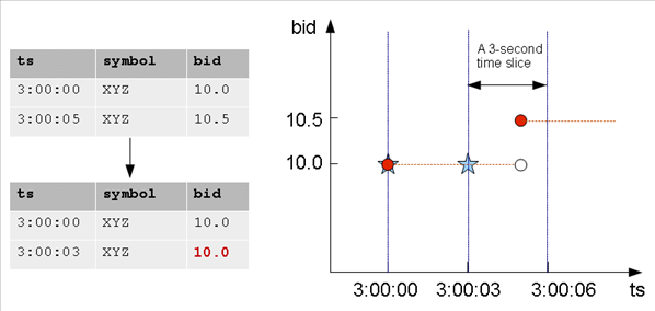
In order to write a query that makes the input rows more uniform, you first need to understand the TIMESERIES clause and time series aggregate functions.
8.1.2 - TIMESERIES clause and aggregates
The SELECT..TIMESERIES clause and time series aggregates help solve the problem of gaps in input records by normalizing the data into 3-second time slices and interpolating the bid price when it finds gaps.
The SELECT..TIMESERIES clause and time series aggregates help solve the problem of gaps in input records by normalizing the data into 3-second time slices and interpolating the bid price when it finds gaps.
TIMESERIES clause
The TIMESERIES clause is an important component of time series analytics computation. It performs gap filling and interpolation (GFI) to generate time slices missing from the input records. The clause applies to the timestamp columns/expressions in the data, and takes the following form:
TIMESERIES slice_time AS 'length_and_time_unit_expression'
OVER ( ... [ window-partition-clause[ , ... ] ]
... ORDER BY time_expression )
... [ ORDER BY table_column [ , ... ] ]
Note
The TIMESERIES clause requires an ORDER BY operation on the timestamp column.Time series aggregate functions
The Timeseries Aggregate (TSA) functions TS_FIRST_VALUE and TS_LAST_VALUE evaluate the values of a given set of variables over time and group those values into a window for analysis and aggregation.
TSA functions process the data that belongs to each time slice. One output row is produced per time slice or per partition per time slice if a partition expression is present.
The following table shows 3-second time slices where:
-
The first two rows fall within the first time slice, which runs from 3:00:00 to 3:00:02. These are the input rows for the TSA function's output for the time slice starting at 3:00:00.
-
The second two rows fall within the second time slice, which runs from 3:00:03 to 3:00:05. These are the input rows for the TSA function's output for the time slice starting at 3:00:03.
The result is the start of each time slice.
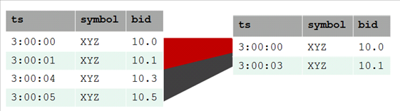
Examples
The following examples compare the values returned with and without the TS_FIRST_VALUE TSA function.
This example shows the TIMESERIES clause without the TS_FIRST_VALUE TSA function.
=> SELECT slice_time, bid FROM TickStore TIMESERIES slice_time AS '3 seconds' OVER(PARTITION by TickStore.bid ORDER BY ts);
This example shows both the TIMESERIES clause and the TS_FIRST_VALUE TSA function. The query returns the values of the bid column, as determined by the specified constant interpolation scheme.
=> SELECT slice_time, TS_FIRST_VALUE(bid, 'CONST') bid FROM TickStore
TIMESERIES slice_time AS '3 seconds' OVER(PARTITION by symbol ORDER BY ts);
Vertica interpolates the last known value and fills in the missing datapoint, returning 10 at 3:00:03:
| First query | Interpolated value | |
|
==> |
slice_time | bid
---------------------+-----
2009-01-01 03:00:00 | 10
2009-01-01 03:00:03 | 10
(2 rows)
|
8.1.3 - Time series rounding
Vertica calculates all time series as equal intervals relative to the timestamp 2000-01-01 00:00:00.
Vertica calculates all time series as equal intervals relative to the timestamp 2000-01-01 00:00:00. Vertica rounds time series timestamps as needed, to conform with this baseline. Start times are also rounded down to the nearest whole unit for the specified interval.
Given this logic, the TIMESERIES clause generates series of timestamps as described in the following sections.
Minutes
Time series of minutes are rounded down to full minutes. For example, the following statement specifies a time span of 00:00:03 ‑ 00:05:50:
=> SELECT ts FROM (
SELECT '2015-01-04 00:00:03'::TIMESTAMP AS tm
UNION
SELECT '2015-01-04 00:05:50'::TIMESTAMP AS tm
) t
TIMESERIES ts AS '1 minute' OVER (ORDER BY tm);
Vertica rounds down the time series start and end times to full minutes, 00:00:00 and 00:05:00, respectively:
ts
---------------------
2015-01-04 00:00:00
2015-01-04 00:01:00
2015-01-04 00:02:00
2015-01-04 00:03:00
2015-01-04 00:04:00
2015-01-04 00:05:00
(6 rows)
Weeks
Because the baseline timestamp 2000-01-01 00:00:00 is a Saturday, all time series of weeks start on Saturday. Vertica rounds down the series start and end timestamps accordingly. For example, the following statement specifies a time span of 12/10/99 ‑ 01/10/00:
=> SELECT ts FROM (
SELECT '1999-12-10 00:00:00'::TIMESTAMP AS tm
UNION
SELECT '2000-01-10 23:59:59'::TIMESTAMP AS tm
) t
TIMESERIES ts AS '1 week' OVER (ORDER BY tm);
The specified time span starts on Friday (12/10/99), so Vertica starts the time series on the preceding Saturday, 12/04/99. The time series ends on the last Saturday within the time span, 01/08/00:
ts
---------------------
1999-12-04 00:00:00
1999-12-11 00:00:00
1999-12-18 00:00:00
1999-12-25 00:00:00
2000-01-01 00:00:00
2000-01-08 00:00:00
(6 rows)
Months
Time series of months are divided into equal 30-day intervals, relative to the baseline timestamp 2000-01-01 00:00:00. For example, the following statement specifies a time span of 09/01/99 ‑ 12/31/00:
=> SELECT ts FROM (
SELECT '1999-09-01 00:00:00'::TIMESTAMP AS tm
UNION
SELECT '2000-12-31 23:59:59'::TIMESTAMP AS tm
) t
TIMESERIES ts AS '1 month' OVER (ORDER BY tm);
Vertica generates a series of 30-day intervals, where each timestamp is rounded up or down, relative to the baseline timestamp:
ts
---------------------
1999-08-04 00:00:00
1999-09-03 00:00:00
1999-10-03 00:00:00
1999-11-02 00:00:00
1999-12-02 00:00:00
2000-01-01 00:00:00
2000-01-31 00:00:00
2000-03-01 00:00:00
2000-03-31 00:00:00
2000-04-30 00:00:00
2000-05-30 00:00:00
2000-06-29 00:00:00
2000-07-29 00:00:00
2000-08-28 00:00:00
2000-09-27 00:00:00
2000-10-27 00:00:00
2000-11-26 00:00:00
2000-12-26 00:00:00
(18 rows)
Years
Time series of years are divided into equal 365-day intervals. If a time span overlaps leap years since or before the baseline timestamp 2000-01-01 00:00:00, Vertica rounds the series timestamps accordingly.
For example, the following statement specifies a time span of 01/01/95 ‑ 05/08/09, which overlaps four leap years, including the baseline timestamp:
=> SELECT ts FROM (
SELECT '1995-01-01 00:00:00'::TIMESTAMP AS tm
UNION
SELECT '2009-05-08'::TIMESTAMP AS tm
) t timeseries ts AS '1 year' over (ORDER BY tm);
Vertica generates a series of timestamps that are rounded up or down, relative to the baseline timestamp:
ts
---------------------
1994-01-02 00:00:00
1995-01-02 00:00:00
1996-01-02 00:00:00
1997-01-01 00:00:00
1998-01-01 00:00:00
1999-01-01 00:00:00
2000-01-01 00:00:00
2000-12-31 00:00:00
2001-12-31 00:00:00
2002-12-31 00:00:00
2003-12-31 00:00:00
2004-12-30 00:00:00
2005-12-30 00:00:00
2006-12-30 00:00:00
2007-12-30 00:00:00
2008-12-29 00:00:00
(16 rows)
8.1.4 - Linear interpolation
Instead of interpolating data points based on the last seen value (constant interpolation), linear interpolation is where Vertica interpolates values in a linear slope based on the specified time slice.
Instead of interpolating data points based on the last seen value (Constant interpolation), linear interpolation is where Vertica interpolates values in a linear slope based on the specified time slice.
The query that follows uses linear interpolation to place the input records in 2-second time slices and return the first bid value for each symbol/time slice combination (the value at the start of the time slice):
=> SELECT slice_time, TS_FIRST_VALUE(bid, 'LINEAR') bid FROM Tickstore
TIMESERIES slice_time AS '2 seconds' OVER(PARTITION BY symbol ORDER BY ts);
slice_time | bid
---------------------+------
2009-01-01 03:00:00 | 10
2009-01-01 03:00:02 | 10.2
2009-01-01 03:00:04 | 10.4
(3 rows)
The following figure illustrates the previous query results, showing the 2-second time gaps (3:00:02 and 3:00:04) in which no input record occurs. Note that the interpolated bid price of XYZ changes to 10.2 at 3:00:02 and 10.3 at 3:00:03 and 10.4 at 3:00:04, all of which fall between the two known data inputs (3:00:00 and 3:00:05). At 3:00:05, the value would change to 10.5.
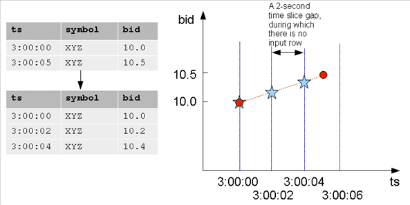
Note
The known data points above are represented by a red dot, and the interpolated values are represented by blue stars.The following is a side-by-side comparison of constant and linear interpolation schemes.
| CONST interpolation | LINEAR interpolation |
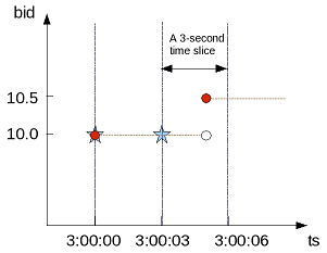 |
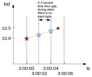 |
8.1.5 - GFI examples
This topic illustrates some of the queries you can write using the constant and linear interpolation schemes.
This topic illustrates some of the queries you can write using the constant and linear interpolation schemes.
Constant interpolation
The first query uses TS_FIRST_VALUE() and the TIMESERIES clause to place the input records in 3-second time slices and return the first bid value for each symbol/time slice combination (the value at the start of the time slice).
Note
The TIMESERIES clause requires an ORDER BY operation on the TIMESTAMP column.=> SELECT slice_time, symbol, TS_FIRST_VALUE(bid) AS first_bid FROM TickStore
TIMESERIES slice_time AS '3 seconds' OVER (PARTITION BY symbol ORDER BY ts);
Because the bid price of stock XYZ is 10.0 at 3:00:03, the first_bid value of the second time slice, which starts at 3:00:03 is till 10.0 (instead of 10.5) because the input value of 10.5 does not occur until 3:00:05. In this case, the interpolated value is inferred from the last value seen on stock XYZ for time 3:00:03:
slice_time | symbol | first_bid
---------------------+--------+-----------
2009-01-01 03:00:00 | XYZ | 10
2009-01-01 03:00:03 | XYZ | 10
(2 rows)
The next example places the input records in 2-second time slices to return the first bid value for each symbol/time slice combination:
=> SELECT slice_time, symbol, TS_FIRST_VALUE(bid) AS first_bid FROM TickStore
TIMESERIES slice_time AS '2 seconds' OVER (PARTITION BY symbol ORDER BY ts);
The result now contains three records in 2-second increments, all of which occur between the first input row at 03:00:00 and the second input row at 3:00:05. Note that the second and third output record correspond to a time slice where there is no input record:
slice_time | symbol | first_bid
---------------------+--------+-----------
2009-01-01 03:00:00 | XYZ | 10
2009-01-01 03:00:02 | XYZ | 10
2009-01-01 03:00:04 | XYZ | 10
(3 rows)
Using the same table schema, the next query uses TS_LAST_VALUE(), with the TIMESERIES clause to return the last values of each time slice (the values at the end of the time slices).
Note
Time series aggregate functions process the data that belongs to each time slice. One output row is produced per time slice or per partition per time slice if a partition expression is present.=> SELECT slice_time, symbol, TS_LAST_VALUE(bid) AS last_bid FROM TickStore
TIMESERIES slice_time AS '2 seconds' OVER (PARTITION BY symbol ORDER BY ts);
Notice that the last value output row is 10.5 because the value 10.5 at time 3:00:05 was the last point inside the 2-second time slice that started at 3:00:04:
slice_time | symbol | last_bid
---------------------+--------+----------
2009-01-01 03:00:00 | XYZ | 10
2009-01-01 03:00:02 | XYZ | 10
2009-01-01 03:00:04 | XYZ | 10.5
(3 rows)
Remember that because constant interpolation is the default, the same results are returned if you write the query using the CONST parameter as follows:
=> SELECT slice_time, symbol, TS_LAST_VALUE(bid, 'CONST') AS last_bid FROM TickStore
TIMESERIES slice_time AS '2 seconds' OVER (PARTITION BY symbol ORDER BY ts);
Linear interpolation
Based on the same input records described in the constant interpolation examples, which specify 2-second time slices, the result of TS_LAST_VALUE with linear interpolation is as follows:
=> SELECT slice_time, symbol, TS_LAST_VALUE(bid, 'linear') AS last_bid FROM TickStore
TIMESERIES slice_time AS '2 seconds' OVER (PARTITION BY symbol ORDER BY ts);
In the results, no last_bid value is returned for the last row because the query specified TS_LAST_VALUE, and there is no data point after the 3:00:04 time slice to interpolate.
slice_time | symbol | last_bid
---------------------+--------+----------
2009-01-01 03:00:00 | XYZ | 10.2
2009-01-01 03:00:02 | XYZ | 10.4
2009-01-01 03:00:04 | XYZ |
(3 rows)
Using multiple time series aggregate functions
Multiple time series aggregate functions can exists in the same query. They share the same gap-filling policy as defined in the TIMESERIES clause; however, each time series aggregate function can specify its own interpolation policy. In the following example, there are two constant and one linear interpolation schemes, but all three functions use a three-second time slice:
=> SELECT slice_time, symbol,
TS_FIRST_VALUE(bid, 'const') fv_c,
TS_FIRST_VALUE(bid, 'linear') fv_l,
TS_LAST_VALUE(bid, 'const') lv_c
FROM TickStore
TIMESERIES slice_time AS '3 seconds' OVER(PARTITION BY symbol ORDER BY ts);
In the following output, the original output is compared to output returned by multiple time series aggregate functions.
|
==> |
|
Using the analytic LAST_VALUE function
Here's an example using LAST_VALUE(), so you can see the difference between it and the GFI syntax.
=> SELECT *, LAST_VALUE(bid) OVER(PARTITION by symbol ORDER BY ts)
AS "last bid" FROM TickStore;
There is no gap filling and interpolation to the output values.
ts | symbol | bid | last bid
---------------------+--------+------+----------
2009-01-01 03:00:00 | XYZ | 10 | 10
2009-01-01 03:00:05 | XYZ | 10.5 | 10.5
(2 rows)
Using slice_time
In a TIMESERIES query, you cannot use the column slice_time in the WHERE clause because the WHERE clause is evaluated before the TIMESERIES clause, and the slice_time column is not generated until the TIMESERIES clause is evaluated. For example, Vertica does not support the following query:
=> SELECT symbol, slice_time, TS_FIRST_VALUE(bid IGNORE NULLS) AS fv
FROM TickStore
WHERE slice_time = '2009-01-01 03:00:00'
TIMESERIES slice_time as '2 seconds' OVER (PARTITION BY symbol ORDER BY ts);
ERROR: Time Series timestamp alias/Time Series Aggregate Functions not allowed in WHERE clause
Instead, you could write a subquery and put the predicate on slice_time in the outer query:
=> SELECT * FROM (
SELECT symbol, slice_time,
TS_FIRST_VALUE(bid IGNORE NULLS) AS fv
FROM TickStore
TIMESERIES slice_time AS '2 seconds'
OVER (PARTITION BY symbol ORDER BY ts) ) sq
WHERE slice_time = '2009-01-01 03:00:00';
symbol | slice_time | fv
--------+---------------------+----
XYZ | 2009-01-01 03:00:00 | 10
(1 row)
Creating a dense time series
The TIMESERIES clause provides a convenient way to create a dense time series for use in an outer join with fact data. The results represent every time point, rather than just the time points for which data exists.
The examples that follow use the same TickStore schema described in Gap filling and interpolation (GFI), along with the addition of a new inner table for the purpose of creating a join:
=> CREATE TABLE inner_table (
ts TIMESTAMP,
bid FLOAT
);
=> CREATE PROJECTION inner_p (ts, bid) as SELECT * FROM inner_table
ORDER BY ts, bid UNSEGMENTED ALL NODES;
=> INSERT INTO inner_table VALUES ('2009-01-01 03:00:02', 1);
=> INSERT INTO inner_table VALUES ('2009-01-01 03:00:04', 2);
=> COMMIT;
You can create a simple union between the start and end range of the timeframe of interest in order to return every time point. This example uses a 1-second time slice:
=> SELECT ts FROM (
SELECT '2009-01-01 03:00:00'::TIMESTAMP AS time FROM TickStore
UNION
SELECT '2009-01-01 03:00:05'::TIMESTAMP FROM TickStore) t
TIMESERIES ts AS '1 seconds' OVER(ORDER BY time);
ts
---------------------
2009-01-01 03:00:00
2009-01-01 03:00:01
2009-01-01 03:00:02
2009-01-01 03:00:03
2009-01-01 03:00:04
2009-01-01 03:00:05
(6 rows)
The next query creates a union between the start and end range of the timeframe using 500-millisecond time slices:
=> SELECT ts FROM (
SELECT '2009-01-01 03:00:00'::TIMESTAMP AS time
FROM TickStore
UNION
SELECT '2009-01-01 03:00:05'::TIMESTAMP FROM TickStore) t
TIMESERIES ts AS '500 milliseconds' OVER(ORDER BY time);
ts
-----------------------
2009-01-01 03:00:00
2009-01-01 03:00:00.5
2009-01-01 03:00:01
2009-01-01 03:00:01.5
2009-01-01 03:00:02
2009-01-01 03:00:02.5
2009-01-01 03:00:03
2009-01-01 03:00:03.5
2009-01-01 03:00:04
2009-01-01 03:00:04.5
2009-01-01 03:00:05
(11 rows)
The following query creates a union between the start- and end-range of the timeframe of interest using 1-second time slices:
=> SELECT * FROM (
SELECT ts FROM (
SELECT '2009-01-01 03:00:00'::timestamp AS time FROM TickStore
UNION
SELECT '2009-01-01 03:00:05'::timestamp FROM TickStore) t
TIMESERIES ts AS '1 seconds' OVER(ORDER BY time) ) AS outer_table
LEFT OUTER JOIN inner_table ON outer_table.ts = inner_table.ts;
The union returns a complete set of records from the left-joined table with the matched records in the right-joined table. Where the query found no match, it extends the right side column with null values:
ts | ts | bid
---------------------+---------------------+-----
2009-01-01 03:00:00 | |
2009-01-01 03:00:01 | |
2009-01-01 03:00:02 | 2009-01-01 03:00:02 | 1
2009-01-01 03:00:03 | |
2009-01-01 03:00:04 | 2009-01-01 03:00:04 | 2
2009-01-01 03:00:05 | |
(6 rows)
8.2 - Null values in time series data
Null values are uncommon inputs for gap-filling and interpolation (GFI) computation.
Null values are uncommon inputs for gap-filling and interpolation (GFI) computation. When null values exist, you can use time series aggregate (TSA) functions
TS_FIRST_VALUE and
TS_LAST_VALUE with IGNORE NULLS to affect output of the interpolated values. TSA functions are treated like their analytic counterparts
FIRST_VALUE and
LAST_VALUE: if the timestamp itself is null, Vertica filters out those rows before gap filling and interpolation occurs.
Constant interpolation with null values
Figure 1 illustrates a default (constant) interpolation result on four input rows where none of the inputs contains a NULL value:
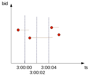 |
Figure 2 shows the same input rows with the addition of another input record whose bid value is NULL, and whose timestamp (ts) value is 3:00:03:
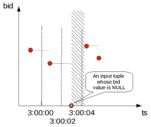 |
For constant interpolation, the bid value starting at 3:00:03 is null until the next non-null bid value appears in time. In Figure 2, the presence of the null row makes the interpolated bid value null in the time interval denoted by the shaded region. If TS_FIRST_VALUE(bid) is evaluated with constant interpolation on the time slice that begins at 3:00:02, its output is non-null. However, TS_FIRST_VALUE(bid) on the next time slice produces null. If the last value of the 3:00:02 time slice is null, the first value for the next time slice (3:00:04) is null. However, if you use a TSA function with IGNORE NULLS, then the value at 3:00:04 is the same value as it was at 3:00:02.
To illustrate, insert a new row into the TickStore table at 03:00:03 with a null bid value, Vertica outputs a row for the 03:00:02 record with a null value but no row for the 03:00:03 input:
=> INSERT INTO tickstore VALUES('2009-01-01 03:00:03', 'XYZ', NULL);
=> SELECT slice_time, symbol, TS_LAST_VALUE(bid) AS last_bid FROM TickStore
-> TIMESERIES slice_time AS '2 seconds' OVER (PARTITION BY symbol ORDER BY ts);
slice_time | symbol | last_bid
---------------------+--------+----------
2009-01-01 03:00:00 | XYZ | 10
2009-01-01 03:00:02 | XYZ |
2009-01-01 03:00:04 | XYZ | 10.5
(3 rows)
If you specify IGNORE NULLS, Vertica fills in the missing data point using a constant interpolation scheme. Here, the bid price at 03:00:02 is interpolated to the last known input record for bid, which was $10 at 03:00:00:
=> SELECT slice_time, symbol, TS_LAST_VALUE(bid IGNORE NULLS) AS last_bid FROM TickStore
TIMESERIES slice_time AS '2 seconds' OVER (PARTITION BY symbol ORDER BY ts);
slice_time | symbol | last_bid
---------------------+--------+----------
2009-01-01 03:00:00 | XYZ | 10
2009-01-01 03:00:02 | XYZ | 10
2009-01-01 03:00:04 | XYZ | 10.5
(3 rows)
Now, if you insert a row where the timestamp column contains a null value, Vertica filters out that row before gap filling and interpolation occurred.
=> INSERT INTO tickstore VALUES(NULL, 'XYZ', 11.2);
=> SELECT slice_time, symbol, TS_LAST_VALUE(bid) AS last_bid FROM TickStore
TIMESERIES slice_time AS '2 seconds' OVER (PARTITION BY symbol ORDER BY ts);
Notice there is no output for the 11.2 bid row:
slice_time | symbol | last_bid
---------------------+--------+----------
2009-01-01 03:00:00 | XYZ | 10
2009-01-01 03:00:02 | XYZ |
2009-01-01 03:00:04 | XYZ | 10.5
(3 rows)
Linear interpolation with null values
For linear interpolation, the interpolated bid value becomes null in the time interval, represented by the shaded region in Figure 3:
 |
In the presence of an input null value at 3:00:03, Vertica cannot linearly interpolate the bid value around that time point.
Vertica takes the closest non null value on either side of the time slice and uses that value. For example, if you use a linear interpolation scheme and do not specify IGNORE NULLS, and your data has one real value and one null, the result is null. If the value on either side is null, the result is null. Therefore, to evaluate TS_FIRST_VALUE(bid) with linear interpolation on the time slice that begins at 3:00:02, its output is null. TS_FIRST_VALUE(bid) on the next time slice remains null.
=> SELECT slice_time, symbol, TS_FIRST_VALUE(bid, 'linear') AS fv_l FROM TickStore
TIMESERIES slice_time AS '2 seconds' OVER (PARTITION BY symbol ORDER BY ts);
slice_time | symbol | fv_l
---------------------+--------+------
2009-01-01 03:00:00 | XYZ | 10
2009-01-01 03:00:02 | XYZ |
2009-01-01 03:00:04 | XYZ |
(3 rows)
9 - Data aggregation
You can use functions such as SUM and COUNT to aggregate the results of GROUP BY queries at one or more levels.
You can use functions such as SUM and COUNT to aggregate the results of GROUP BY queries at one or more levels.
9.1 - Single-level aggregation
The simplest GROUP BY queries aggregate data at a single level.
The simplest GROUP BY queries aggregate data at a single level. For example, a table might contain the following information about family expenses:
-
Category
-
Amount spent on that category during the year
-
Year
Table data might look like this:
=> SELECT * FROM expenses ORDER BY Category;
Year | Category | Amount
------+------------+--------
2005 | Books | 39.98
2007 | Books | 29.99
2008 | Books | 29.99
2006 | Electrical | 109.99
2005 | Electrical | 109.99
2007 | Electrical | 229.98
You can use aggregate functions to get the total expenses per category or per year:
=> SELECT SUM(Amount), Category FROM expenses GROUP BY Category;
SUM | Category
---------+------------
99.96 | Books
449.96 | Electrical
=> SELECT SUM(Amount), Year FROM expenses GROUP BY Year;
SUM | Year
--------+------
149.97 | 2005
109.99 | 2006
29.99 | 2008
259.97 | 2007
9.2 - Multi-level aggregation
Over time, tables that are updated frequently can contain large amounts of data.
Over time, tables that are updated frequently can contain large amounts of data. Using the simple table shown earlier, suppose you want a multilevel query, like the number of expenses per category per year.
The following query uses the ROLLUP aggregation with the SUM function to calculate the total expenses by category and the overall expenses total. The NULL fields indicate subtotal values in the aggregation.
-
When only the
Yearcolumn isNULL, the subtotal is for all theCategoryvalues. -
When both the
YearandCategorycolumns areNULL, the subtotal is for allAmountvalues for both columns.
Using the ORDER BY clause orders the results by expense category, the year the expenses took place, and the GROUP BY level that the GROUPING_ID function creates:
=> SELECT Category, Year, SUM(Amount) FROM expenses
GROUP BY ROLLUP(Category, Year) ORDER BY Category, Year, GROUPING_ID();
Category | Year | SUM
------------+------+--------
Books | 2005 | 39.98
Books | 2007 | 29.99
Books | 2008 | 29.99
Books | | 99.96
Electrical | 2005 | 109.99
Electrical | 2006 | 109.99
Electrical | 2007 | 229.98
Electrical | | 449.96
| | 549.92
Similarly, the following query calculates the total sales by year and the overall sales total and then uses the ORDER BY clause to sort the results:
=> SELECT Category, Year, SUM(Amount) FROM expenses
GROUP BY ROLLUP(Year, Category) ORDER BY 2, 1, GROUPING_ID();
Category | Year | SUM
------------+------+--------
Books | 2005 | 39.98
Electrical | 2005 | 109.99
| 2005 | 149.97
Electrical | 2006 | 109.99
| 2006 | 109.99
Books | 2007 | 29.99
Electrical | 2007 | 229.98
| 2007 | 259.97
Books | 2008 | 29.99
| 2008 | 29.99
| | 549.92
(11 rows)
You can use the CUBE aggregate to perform all possible groupings of the category and year expenses. The following query returns all possible groupings, ordered by grouping:
=> SELECT Category, Year, SUM(Amount) FROM expenses
GROUP BY CUBE(Category, Year) ORDER BY 1, 2, GROUPING_ID();
Category | Year | SUM
------------+------+--------
Books | 2005 | 39.98
Books | 2007 | 29.99
Books | 2008 | 29.99
Books | | 99.96
Electrical | 2005 | 109.99
Electrical | 2006 | 109.99
Electrical | 2007 | 229.98
Electrical | | 449.96
| 2005 | 149.97
| 2006 | 109.99
| 2007 | 259.97
| 2008 | 29.99
| | 549.92
The results include subtotals for each category and each year and a total ($549.92) for all transactions, regardless of year or category.
ROLLUP, CUBE, and GROUPING SETS generate NULL values in grouping columns to identify subtotals. If table data includes NULL values, differentiating these from NULL values in subtotals can sometimes be challenging.
In the preceding output, the NULL values in the Year column indicate that the row was grouped on the Category column, rather than on both columns. In this case, ROLLUP added the NULL value to indicate the subtotal row.
9.3 - Aggregates and functions for multilevel grouping
Vertica provides several aggregates and functions that group the results of a GROUP BY query at multiple levels.
Vertica provides several aggregates and functions that group the results of a GROUP BY query at multiple levels.
Aggregates for multilevel grouping
Use the following aggregates for multilevel grouping:
-
ROLLUPautomatically performs subtotal aggregations. ROLLUP performs one or more aggregations across multiple dimensions, at different levels. -
CUBEperforms the aggregation for all permutations of the CUBE expression that you specify. -
GROUPING SETSlet you specify which groupings of aggregations you need.
You can use CUBE or ROLLUP expressions inside GROUPING SETS expressions. Otherwise, you cannot nest multilevel aggregate expressions.
Grouping functions
You use one of the following three grouping functions with ROLLUP, CUBE, and GROUPING SETS:
-
GROUP_ID returns one or more numbers, starting with zero (0), to uniquely identify duplicate sets.
-
GROUPING_ID produces a unique ID for each grouping combination.
-
GROUPING identifies for each grouping combination whether a column is a part of this grouping. This function also differentiates NULL values in the data from NULL grouping subtotals.
These functions are typically used with multilevel aggregates.
9.4 - Aggregate expressions for GROUP BY
You can include CUBE and ROLLUP aggregates within a GROUPING SETS aggregate.
You can include CUBE and ROLLUP aggregates within a GROUPING SETS aggregate. Be aware that the CUBE and ROLLUP aggregates can result in a large amount of output. However, you can avoid large outputs by using GROUPING SETS to return only specified results.
...GROUP BY a,b,c,d,ROLLUP(a,b)...
...GROUP BY a,b,c,d,CUBE((a,b),c,d)...
You cannot include any aggregates in a CUBE or ROLLUP aggregate expression.
You can append multiple GROUPING SETS, CUBE, or ROLLUP aggregates in the same query.
...GROUP BY a,b,c,d,CUBE(a,b),ROLLUP (c,d)...
...GROUP BY a,b,c,d,GROUPING SETS ((a,d),(b,c),CUBE(a,b));...
...GROUP BY a,b,c,d,GROUPING SETS ((a,d),(b,c),(a,b),(a),(b),())...
9.5 - Pre-aggregating data in projections
Queries that use aggregate functions such as SUM and COUNT can perform more efficiently when they use projections that already contain the aggregated data.
Queries that use aggregate functions such as SUM and COUNT can perform more efficiently when they use projections that already contain the aggregated data. This improved efficiency is especially true for queries on large quantities of data.
For example, a power grid company reads 30 million smart meters that provide data at five-minute intervals. The company records each reading in a database table. Over a given year, three trillion records are added to this table.
The power grid company can analyze these records with queries that include aggregate functions to perform the following tasks:
-
Establish usage patterns.
-
Detect fraud.
-
Measure correlation to external events such as weather patterns or pricing changes.
To optimize query response time, you can create an aggregate projection, which stores the data is stored after it is aggregated.
Aggregate projections
Vertica provides several types of projections for storing data that is returned from aggregate functions or expressions:
-
Live aggregate projection: Projection that contains columns with values that are aggregated from columns in its anchor table. You can also define live aggregate projections that include user-defined transform functions.
-
Top-K projection: Type of live aggregate projection that returns the top
krows from a partition of selected rows. Create a Top-K projection that satisfies the criteria for a Top-K query. -
Projection that pre-aggregates UDTF results: Live aggregate projection that invokes user-defined transform functions (UDTFs). To minimize overhead when you query those projections of this type, Vertica processes the UDTF functions in the background and stores their results on disk.
-
Projection that contains expressions: Projection with columns whose values are calculated from anchor table columns.
Recommended use
-
Aggregate projections are most useful for queries against large sets of data.
-
For optimal query performance, the size of LAP projections should be a small subset of the anchor table—ideally, between 1 and 10 percent of the anchor table, or smaller, if possible.
Restrictions
-
MERGE operations must be optimized if they are performed on target tables that have live aggregate projections.
-
You cannot update or delete data in temporary tables with live aggregate projections.
Requirements
In the event of manual recovery from an unclean database shutdown, live aggregate projections might require some time to refresh.
9.5.1 - Live aggregate projections
A live aggregate projection contains columns with values that are aggregated from columns in its anchor table. When you load data into the table, Vertica aggregates the data before loading it into the live aggregate projection. On subsequent loads—for example, through INSERTor COPY—Vertica recalculates aggregations with the new data and updates the projection.
9.5.1.1 - Functions supported for live aggregate projections
Vertica can aggregate results in live aggregate projections from the following aggregate functions:.
Vertica can aggregate results in live aggregate projections from the following aggregate functions:
Aggregate functions with DISTINCT
Live aggregate projections can support queries that include aggregate functions qualified with the keyword DISTINCT. The following requirements apply:
-
The aggregated expression must evaluate to a non-constant.
-
The projection's
GROUP BYclause must specify the aggregated expression.
For example, the following query uses SUM(DISTINCT) to calculate the total of all unique salaries in a given region:
SELECT customer_region, SUM(DISTINCT annual_income)::INT
FROM customer_dimension GROUP BY customer_region;
This query can use the following live aggregate projection, which specifies the aggregated column (annual_income) in its GROUP BY clause:
CREATE PROJECTION public.TotalRegionalIncome
(
customer_region,
annual_income,
Count
)
AS
SELECT customer_dimension.customer_region,
customer_dimension.annual_income,
count(*) AS Count
FROM public.customer_dimension
GROUP BY customer_dimension.customer_region,
customer_dimension.annual_income
;
Note
This projection includes the aggregate functionCOUNT, which here serves no logical objective; it is included only because live aggregate projections require at least one aggregate function.
9.5.1.2 - Creating live aggregate projections
You define a live aggregate projection with the following syntax:.
You define a live aggregate projection with the following syntax:
=> CREATE PROJECTION proj-name AS
SELECT select-expression FROM table
GROUP BY group-expression;
For full syntax options, see CREATE PROJECTION.
For example:
=> CREATE PROJECTION clicks_agg AS
SELECT page_id, click_time::DATE click_date, COUNT(*) num_clicks FROM clicks
GROUP BY page_id, click_time::DATE KSAFE 1;
For an extended discussion, see Live aggregate projection example.
Requirements
The following requirements apply to live aggregate projections:
-
The projection cannot be unsegmented.
Note
Unless the CREATE PROJECTION statement or its anchor table DDL specify otherwise, all projections are segmented by default. -
SELECT and GROUP BY columns must be in the same order. GROUP BY expressions must be at the beginning of the SELECT list.
Restrictions
The following restrictions apply to live aggregate projections:
-
MERGE operations must be optimized if they are performed on target tables that have live aggregate projections.
-
Live aggregate projections can reference only one table.
-
Vertica does not regard live aggregate projections as superprojections, even those that include all table columns.
-
You cannot modify the anchor table metadata of columns that are included in live aggregate projections—for example, a column's data type or default value. You also cannot drop these columns. To make these changes, first drop all live aggregate and Top-K projections that are associated with the table.
Note
One exception applies: You can set and drop NOT NULL on columns that are included in a live aggregate projection.
9.5.1.3 - Live aggregate projection example
This example shows how you can track user clicks on a given web page using the following clicks table:.
This example shows how you can track user clicks on a given web page using the following clicks table:
=> CREATE TABLE clicks(
user_id INTEGER,
page_id INTEGER,
click_time TIMESTAMP NOT NULL);
You can aggregate user-specific activity with the following query:
=> SELECT page_id, click_time::DATE click_date, COUNT(*) num_clicks FROM clicks
WHERE click_time::DATE = '2015-04-30'
GROUP BY page_id, click_time::DATE ORDER BY num_clicks DESC;
To facilitate performance of this query, create a live aggregate projection that counts the number of clicks per user:
=> CREATE PROJECTION clicks_agg AS
SELECT page_id, click_time::DATE click_date, COUNT(*) num_clicks FROM clicks
GROUP BY page_id, click_time::DATE KSAFE 1;
When you query the clicks table on user clicks, Vertica typically directs the query to the live aggregate projection clicks_agg. As additional data is loaded into clicks, Vertica pre-aggregates the new data and updates clicks_agg, so queries always return with the latest data.
For example:
=> SELECT page_id, click_time::DATE click_date, COUNT(*) num_clicks FROM clicks
WHERE click_time::DATE = '2015-04-30' GROUP BY page_id, click_time::DATE
ORDER BY num_clicks DESC;
page_id | click_date | num_clicks
---------+------------+------------
2002 | 2015-04-30 | 10
3003 | 2015-04-30 | 3
2003 | 2015-04-30 | 1
2035 | 2015-04-30 | 1
12034 | 2015-04-30 | 1
(5 rows)
9.5.2 - Top-k projections
A Top-K query returns the top k rows from partitions of selected rows.
A Top-K query returns the top k rows from partitions of selected rows. Top-K projections can significantly improve performance of Top-K queries. For example, you can define a table that stores gas meter readings with three columns: gas meter ID, time of meter reading, and the read value:
=> CREATE TABLE readings (
meter_id INT,
reading_date TIMESTAMP,
reading_value FLOAT);
Given this table, the following Top-K query returns the five most recent meter readings for a given meter:
SELECT meter_id, reading_date, reading_value FROM readings
LIMIT 5 OVER (PARTITION BY meter_id ORDER BY reading_date DESC);
To improve the performance of this query, you can create a Top-K projection, which is a special type of live aggregate projection:
=> CREATE PROJECTION readings_topk (meter_id, recent_date, recent_value)
AS SELECT meter_id, reading_date, reading_value FROM readings
LIMIT 5 OVER (PARTITION BY meter_id ORDER BY reading_date DESC);
After you create this Top-K projection and load its data (through START_REFRESH or REFRESH), Vertica typically redirects the query to the projection and returns with the pre-aggregated data.
9.5.2.1 - Creating top-k projections
You define a Top-K projection with the following syntax:.
You define a Top-K projection with the following syntax:
CREATE PROJECTION proj-name [(proj-column-spec)]
AS SELECT select-expression FROM table
LIMIT num-rows OVER (PARTITION BY expression ORDER BY column-expr);
For full syntax options, see CREATE PROJECTION.
For example:
=> CREATE PROJECTION readings_topk (meter_id, recent_date, recent_value)
AS SELECT meter_id, reading_date, reading_value FROM readings
LIMIT 5 OVER (PARTITION BY meter_id ORDER BY reading_date DESC);
For an extended discussion, see Top-k projection examples.
Requirements
The following requirements apply to Top-K projections:
-
The projection cannot be unsegmented.
-
The window partition clause must use
PARTITION BY. -
Columns in
PARTITION BYandORDER BYclauses must be the first columns specified in theSELECTlist. -
You must use the
LIMIToption to create a Top-K projection, instead of subqueries. For example, the followingSELECTstatements are equivalent:=> SELECT symbol, trade_time last_trade, price last_price FROM ( SELECT symbol, trade_time, price, ROW_NUMBER() OVER(PARTITION BY symbol ORDER BY trade_time DESC) rn FROM trades) trds WHERE rn <=1; => SELECT symbol, trade_time last_trade, price last_price FROM trades LIMIT 1 OVER(PARTITION BY symbol ORDER BY trade_time DESC);Both return the same results:
symbol | last_trade | last_price ------------------+-----------------------+------------ AAPL | 2011-11-10 10:10:20.5 | 108.4000 HPQ | 2012-10-10 10:10:10.4 | 42.0500 (2 rows)A Top-K projection that pre-aggregates data for use by both queries must include the
LIMIToption:=> CREATE PROJECTION trades_topk AS SELECT symbol, trade_time last_trade, price last_price FROM trades LIMIT 1 OVER(PARTITION BY symbol ORDER BY trade_time DESC);
Restrictions
The following restrictions apply to Top-K projections:
-
Top-K projections can reference only one table.
-
Vertica does not regard Top-K projections as superprojections, even those that include all table columns.
-
You cannot modify the anchor table metadata of columns that are included in Top-K projections—for example, a column's data type or default value. You also cannot drop these columns. To make these changes, first drop all live aggregate and Top-K projections that are associated with the table.
Note
One exception applies: You can set and drop NOT NULL on columns that are included in a live aggregate projection.
9.5.2.2 - Top-k projection examples
The following examples show how to query a table with two Top-K projections for the most-recent trade and last trade of the day for each stock symbol.
The following examples show how to query a table with two Top-K projections for the most-recent trade and last trade of the day for each stock symbol.
-
Create a table that contains information about individual stock trades:
-
Stock symbol
-
Timestamp
-
Price per share
-
Number of shares
=> CREATE TABLE trades( symbol CHAR(16) NOT NULL, trade_time TIMESTAMP NOT NULL, price NUMERIC(12,4), volume INT ) PARTITION BY (EXTRACT(year from trade_time) * 100 + EXTRACT(month from trade_time)); -
-
Load data into the table:
INSERT INTO trades VALUES('AAPL','2010-10-10 10:10:10'::TIMESTAMP,100.00,100); INSERT INTO trades VALUES('AAPL','2010-10-10 10:10:10.3'::TIMESTAMP,101.00,100); INSERT INTO trades VALUES ('AAPL','2011-10-10 10:10:10.5'::TIMESTAMP,106.1,1000); INSERT INTO trades VALUES ('AAPL','2011-10-10 10:10:10.2'::TIMESTAMP,105.2,500); INSERT INTO trades VALUES ('HPQ','2012-10-10 10:10:10.2'::TIMESTAMP,42.01,400); INSERT INTO trades VALUES ('HPQ','2012-10-10 10:10:10.3'::TIMESTAMP,42.02,1000); INSERT INTO trades VALUES ('HPQ','2012-10-10 10:10:10.4'::TIMESTAMP,42.05,100); COMMIT; -
Create two Top-K projections that obtain the following information from the
tradestable:For each stock symbol, return the most recent trade.
=> CREATE PROJECTION trades_topk_a AS SELECT symbol, trade_time last_trade, price last_price FROM trades LIMIT 1 OVER(PARTITION BY symbol ORDER BY trade_time DESC); => SELECT symbol, trade_time last_trade, price last_price FROM trades LIMIT 1 OVER(PARTITION BY symbol ORDER BY trade_time DESC); symbol | last_trade | last_price ------------------+-----------------------+------------ HPQ | 2012-10-10 10:10:10.4 | 42.0500 AAPL | 2011-10-10 10:10:10.5 | 106.1000 (2 rows)
For each stock symbol, return the last trade on each trading day.=> CREATE PROJECTION trades_topk_b AS SELECT symbol, trade_time::DATE trade_date, trade_time, price close_price, volume FROM trades LIMIT 1 OVER(PARTITION BY symbol, trade_time::DATE ORDER BY trade_time DESC); => SELECT symbol, trade_time::DATE trade_date, trade_time, price close_price, volume FROM trades LIMIT 1 OVER(PARTITION BY symbol, trade_time::DATE ORDER BY trade_time DESC); symbol | trade_date | trade_time | close_price | volume ------------------+------------+-----------------------+-------------+-------- HPQ | 2012-10-10 | 2012-10-10 10:10:10.4 | 42.0500 | 100 AAPL | 2011-10-10 | 2011-10-10 10:10:10.5 | 106.1000 | 1000 AAPL | 2010-10-10 | 2010-10-10 10:10:10.3 | 101.0000 | 100 (3 rows)
In each scenario, Vertica redirects queries on the trades table to the appropriate Top-K projection and returns the aggregated data from them. As additional data is loaded into this table, Vertica pre-aggregates the new data and updates the Top-K projections, so queries always return with the latest data.
9.5.3 - Pre-aggregating UDTF results
CREATE PROJECTION can define live aggregate projections that invoke user-defined transform functions (UDTFs).
CREATE PROJECTION can define live aggregate projections that invoke user-defined transform functions (UDTFs). To minimize overhead when you query those projections, Vertica processes these functions in the background and stores their results on disk.
Important
Currently, live aggregate projections can only reference UDTFs that are developed in C++.Defining projections with UDTFs
The projection definition characterizes UDTFs in one of two ways:
-
Identifies the UDTF as a pre-pass UDTF, which transforms newly loaded data before it is stored in the projection ROS containers.
-
Identifies the UDTF as a batch UDTF, which aggregates and stores projection data.
The projection definition identifies a UDTF as a pre-pass UDTF or batch UDTF in its window partition clause, through the keywords PREPASS or BATCH. A projection can specify one pre-pass or batch UDTF or include both (see UDTF Specification Options).
In all cases, the projection is implicitly segmented and ordered on the PARTITION BY columns.
UDTF specification options
Projections can invoke batch and pre-pass UDTFs singly or in combination.
Single pre-pass UDTF
Vertica invokes the pre-pass UDTF when you load data into the projection's anchor table—for example through COPY or INSERT statements. A pre-pass UDTF transforms the new data and then stores the transformed data in the projection's ROS containers.
Use the following syntax:
CREATE PROJECTION [ IF NOT EXISTS ] [[database.]schema.]projection
[ (
{ projection-column | grouped-clause
[ ENCODING encoding-type ]
[ ACCESSRANK integer ] }[,...]
) ]
AS SELECT { table-column | expr-with-table-columns }[,...], prepass-udtf(prepass-args)
OVER (PARTITION PREPASS BY partition-column-expr[,...])
[ AS (prepass-output-columns) ] FROM table [[AS] alias]
Single batch UDTF
When invoked singly, a batch UDTF transforms and aggregates projection data on mergeout, data load, and query operations. The UDTF stores aggregated results in the projection's ROS containers. Aggregation is cumulative across mergeout and load operations, and is completed (if necessary) on query execution.
Use the following syntax:
CREATE PROJECTION [ IF NOT EXISTS ] [[database.]schema.]projection
[ (
{ projection-column | grouped-clause
[ ENCODING encoding-type ]
[ ACCESSRANK integer ] }[,...]
) ]
AS SELECT { table-column | expr-with-table-columns }[,...], batch-udtf(batch-args)
OVER (PARTITION BATCH BY partition-column-expr[,...])
[ AS (batch-output-columns) FROM table [ [AS] alias ]
Combined pre-pass and batch UDTFs
You can define a projection with a subquery that invokes a pre-pass UDTF. The pre-pass UDTF returns transformed data to the outer batch query. The batch UDTF then iteratively aggregates results across mergeout operations. It completes aggregation (if necessary) on query execution.
Use the following syntax:
CREATE PROJECTION [ IF NOT EXISTS ] [[database.]schema.]projection
[ (
{ projection-column | grouped-clause
[ ENCODING encoding-type ]
[ ACCESSRANK integer ] }[,...]
) ]
AS SELECT { table-column | expr-with-table-columns }[,...], batch-udtf(batch-args)
OVER (PARTITION BATCH BY partition-column-expr[,...]) [ AS (batch-output-columns) ] FROM (
SELECT { table-column | expr-with-table-columns }[,...], prepass-udtf (prepass-args)
OVER (PARTITION PREPASS BY partition-column-expr[,...]) [ AS (prepass-output-columns) ] FROM table ) sq-ref
Important
The outer batch UDTF argumentsbatch‑args must exactly match the output columns returned by the pre-pass UDTF, in name and order.
Examples
Single pre-pass UDTF
The following example shows how to use the UDTF text_index, which extracts from a text document strings that occur more than once.
The following projection specifies to invoke text_index as a pre-pass UDTF:
=> CREATE TABLE documents ( doc_id INT PRIMARY KEY, text VARCHAR(140));
=> CREATE PROJECTION index_proj (doc_id, text)
AS SELECT doc_id, text_index(doc_id, text)
OVER (PARTITION PREPASS BY doc_id) FROM documents;
The UDTF is invoked whenever data is loaded into the anchor table documents. text_index transforms the newly loaded data, and Vertica stores the transformed data in the live aggregate projection ROS containers.
So, if you load the following data into documents:
=> INSERT INTO documents VALUES
(100, 'A SQL Query walks into a bar. In one corner of the bar are two tables.
The Query walks up to the tables and asks - Mind if I join you?');
OUTPUT
--------
1
(1 row)
text_index transforms the newly loaded data and stores it in the projection ROS containers. When you query the projection, it returns with the following results:
doc_id | frequency | term
-------+-----------+--------------
100 | 2 | bar
100 | 2 | Query
100 | 2 | tables
100 | 2 | the
100 | 2 | walks
Combined Pre-Pass and Batch UDTFs
The following projection specifies pre-pass and batch UDTFs stv_intersect and aggregate_classified_points, respectively:
CREATE TABLE points( point_id INTEGER, point_type VARCHAR(10), coordinates GEOMETRY(100));
CREATE PROJECTION aggregated_proj
AS SELECT point_type, aggregate_classified_points( sq.point_id, sq.polygon_id)
OVER (PARTITION BATCH BY point_type) AS some_alias
FROM
(SELECT point_type, stv_intersect(
point_id, coordinates USING PARAMETERS index='polygons' )
OVER (PARTITION PREPASS BY point_type) AS (point_id, polygon_id) FROM points) sq;
The pre-pass query UDTF stv_intersect returns its results (a set of point and matching polygon IDs) to the outer batch query. The outer batch query then invokes the UDTF aggregate_classified_points. Vertica aggregates the result set that is returned by aggregate_classified_points whenever a mergeout operation consolidates projection data. Final aggregation (if necessary) occurs when the projection is queried.
The batch UDTF arguments must exactly match the output columns returned by the pre-pass UDTF stv_intersect, in name and order. In this example, the pre-pass subquery explicitly names the pre-pass UDTF output columns point_id and polygon_id. Accordingly, the batch UDTF arguments match them in name and order: sq.point_id and sq.polygon_id.
9.5.4 - Aggregating data through expressions
You can create projections where one or more columns are defined by expressions.
You can create projections where one or more columns are defined by expressions. An expression can reference one or more anchor table columns. For example, the following table contains two integer columns, a and b:
=> CREATE TABLE values (a INT, b INT);
You can create a projection with an expression that calculates the value of column c as the product of a and b:
=> CREATE PROJECTION values_product (a, b, c)
AS SELECT a, b, a*b FROM values SEGMENTED BY HASH(a) ALL NODES KSAFE;
When you load data into this projection, Vertica resolves the expression a*b in column c. You can then query the projection instead of the anchor table. Vertica returns the pre-calculated data and avoids the overhead otherwise incurred by resource-intensive computations.
Using expressions in projections also lets you sort or segment data on the calculated results of an expression instead of sorting on single column values.
Note
If a projection with expressions also includes aggregate functions such as SUM or COUNT, Vertica treats it like a live aggregate projection.Support for user-defined scalar functions
Important
Currently, support for pre-aggregating UDSF results is limited to C++.Vertica treats user-defined scalar functions (UDSFs) like other expressions. On each load operation, the UDSF is invoked and returns its results. Vertica stores these results on disk, and returns them when you query the projection directly.
In the following example, the projection points_p1 specifies the UDSF zorder, which is invoked whenever data is loaded in the anchor table points. When data is loaded into the projection, Vertica invokes this function and stores its results for fast access by future queries.
=> CREATE TABLE points(point_id INTEGER, lat NUMERIC(12,9), long NUMERIC(12,9));
=> CREATE PROJECTION points_p1
AS SELECT point_id, lat, long, zorder(lat, long) zorder FROM points
ORDER BY zorder(lat, long) SEGMENTED BY hash(point_id) ALL NODES;
Requirements
-
Any
ORDER BYexpression must be in theSELECTlist. -
All projection columns must be named.
Restrictions
-
MERGE operations must be optimized if they are performed on target tables that have live aggregate projections.
-
Unlike live aggregate projections, Vertica does not redirect queries with expressions to an equivalent existing projection.
-
Projection expressions must be immutable—that is, they must always return the same result. For example, a projection cannot include expressions that use
TO CHAR(depends on locale) orRANDOM(returns different value at each invocation). -
Projection expressions cannot include Vertica meta-functions such as
ADVANCE_EPOCH,ANALYZE_STATISTICS,EXPORT_TABLES, orSTART_REFRESH.
9.5.4.1 - Querying data through expressions example
The following example uses a table that contains two integer columns, a and b:.
The following example uses a table that contains two integer columns, a and b:
=> CREATE TABLE values (a INT, b INT);
You can create a projection with an expression that calculates the value of column c as the product of a and b:
=> CREATE PROJECTION values_product (a, b, c)
AS SELECT a, b, a*b FROM values SEGMENTED BY HASH(a) ALL NODES KSAFE;
=> COPY values FROM STDIN DELIMITER ',' DIRECT;
Enter data to be copied followed by a newline.
End with a backslash and a period on a line by itself.
>> 3,11
>> 3,55
>> 8,9
>> 8,23
>> 16,41
>> 22,111
>> \.
=>
To query this projection, use the name that Vertica assigns to it or to its buddy projections. For example, the following queries target different instances of the projection defined earlier, and return the same results:
=> SELECT * FROM values_product_b0;
=> SELECT * FROM values_product_b1;
The following example queries the anchor table:
=> SELECT * FROM values;
a | b
----+-----
3 | 11
3 | 55
8 | 9
8 | 23
16 | 41
22 | 111
Given the projection created earlier, querying that projection returns the following values:
VMart=> SELECT * FROM values_product_b0;
a | b | product
----+-----+---------
3 | 11 | 33
3 | 55 | 165
8 | 9 | 72
8 | 23 | 184
16 | 41 | 656
22 | 111 | 2442
9.5.5 - Aggregation information in system tables
You can query the following system table fields for information about live aggregate projections, Top-K projections, and projections with expressions:.
You can query the following system table fields for information about live aggregate projections, Top-K projections, and projections with expressions: