This is the multi-page printable view of this section.
Click here to print.
Return to the regular view of this page.
Data types
The following table summarizes the internal data types that Vertica supports.
The following table summarizes the internal data types that Vertica supports. It also shows the default placement of null values in projections. The Size column lists uncompressed bytes.
|
Data Type |
Size / bytes |
Description |
NULL Sorting |
|
Binary |
|
BINARY |
1 to 65,000 |
Fixed-length binary string |
NULLS LAST |
|
VARBINARY (synonyms: BYTEA, RAW) |
1 to 65,000 |
Variable-length binary string |
NULLS LAST |
|
LONG VARBINARY |
1 to 32,000,000 |
Long variable-length binary string |
NULLS LAST |
|
Boolean |
|
BOOLEAN |
1 |
True or False or NULL |
NULLS LAST |
|
Character / Long |
|
CHAR |
1 to 65,000 |
Fixed-length character string |
NULLS LAST |
|
VARCHAR |
1 to 65,000 |
Variable-length character string |
NULLS LAST |
|
LONG VARCHAR |
1 to 32,000,000 |
Long variable-length character string |
NULLS LAST |
|
Date/Time |
|
DATE |
8 |
A month, day, and year |
NULLS FIRST |
|
TIME |
8 |
A time of day without timezone |
NULLS FIRST |
|
TIME WITH TIMEZONE |
8 |
A time of day with timezone |
NULLS FIRST |
|
TIMESTAMP (synonyms: DATETIME, SMALLDATETIME) |
8 |
A date and time without timezone |
NULLS FIRST |
|
TIMESTAMP WITH TIMEZONE |
8 |
A date and time with timezone |
NULLS FIRST |
|
INTERVAL |
8 |
The difference between two points in time |
NULLS FIRST |
|
INTERVAL DAY TO SECOND |
8 |
An interval measured in days and seconds |
NULLS FIRST |
|
INTERVAL YEAR TO MONTH |
8 |
An interval measured in years and months |
NULLS FIRST |
|
Approximate Numeric |
|
DOUBLE PRECISION |
8 |
Signed 64-bit IEEE floating point number, requiring 8 bytes of storage |
NULLS LAST |
|
FLOAT |
8 |
Signed 64-bit IEEE floating point number, requiring 8 bytes of storage |
NULLS LAST |
|
FLOAT(n) |
8 |
Signed 64-bit IEEE floating point number, requiring 8 bytes of storage |
NULLS LAST |
|
FLOAT8 |
8 |
Signed 64-bit IEEE floating point number, requiring 8 bytes of storage |
NULLS LAST |
|
REAL |
8 |
Signed 64-bit IEEE floating point number, requiring 8 bytes of storage |
NULLS LAST |
|
Exact Numeric |
|
INTEGER |
8 |
Signed 64-bit integer, requiring 8 bytes of storage |
NULLS FIRST |
|
INT |
8 |
Signed 64-bit integer, requiring 8 bytes of storage |
NULLS FIRST |
|
BIGINT |
8 |
Signed 64-bit integer, requiring 8 bytes of storage |
NULLS FIRST |
|
INT8 |
8 |
Signed 64-bit integer, requiring 8 bytes of storage |
NULLS FIRST |
|
SMALLINT |
8 |
Signed 64-bit integer, requiring 8 bytes of storage |
NULLS FIRST |
|
TINYINT |
8 |
Signed 64-bit integer, requiring 8 bytes of storage |
NULLS FIRST |
|
DECIMAL |
8+ |
8 bytes for the first 18 digits of precision, plus 8 bytes for each additional 19 digits |
NULLS FIRST |
|
NUMERIC |
8+ |
8 bytes for the first 18 digits of precision, plus 8 bytes for each additional 19 digits |
NULLS FIRST |
|
NUMBER |
8+ |
8 bytes for the first 18 digits of precision, plus 8 bytes for each additional 19 digits |
NULLS FIRST |
|
MONEY |
8+ |
8 bytes for the first 18 digits of precision, plus 8 bytes for each additional 19 digits |
NULLS FIRST |
|
Spatial |
|
GEOMETRY |
1 to 10,000,000 |
Coordinates expressed as (x,y) pairs, defined in the Cartesian plane. |
NULLS LAST |
|
GEOGRAPHY |
1 to 10,000,000 |
Coordinates expressed in longitude/latitude angular values, measured in degrees |
NULLS LAST |
|
UUID |
|
UUID |
16 |
Stores universally unique identifiers (UUIDs). |
NULLS FIRST |
|
Complex |
|
ARRAY |
1 to 32,000,000 |
Collection of values of a primitive or complex type. |
Native array: same as the element type
Non-native array: cannot be used to order projections
|
|
ROW |
1 to 32,000,000 |
Structure of property-value pairs. |
Cannot be used to order projections |
|
SET |
1 to 32,000,000 |
Collection of unique values of a primitive type. |
Same as the primitive type |
1 - Binary data types (BINARY and VARBINARY)
Store raw-byte data, such as IP addresses, up to bytes.
Store raw-byte data, such as IP addresses, up to 65000 bytes. The BINARY and BINARY VARYING (VARBINARY) data types are collectively referred to as binary string types and the values of binary string types are referred to as binary strings. A binary string is a sequence of octets or bytes.
BYTEA and RAW are synonyms for VARBINARY.
Syntax
BINARY ( length )
{ VARBINARY | BINARY VARYING | BYTEA | RAW } ( max-length )
Arguments
length, max-length- The length of the string or column width, in bytes (octets).
BINARY and VARBINARY data types
BINARY and VARBINARY data types have the following attributes:
-
BINARY: A fixed-width string of length bytes, where the number of bytes is declared as an optional specifier to the type. If length is omitted, the default is 1. Where necessary, values are right-extended to the full width of the column with the zero byte. For example:
=> SELECT TO_HEX('ab'::BINARY(4));
  to_hex
----------
 61620000
-
VARBINARY: A variable-width string up to a length of max-length bytes, where the maximum number of bytes is declared as an optional specifier to the type. The default is the default attribute size, which is 80, and the maximum length is 65000 bytes. VARBINARY values are not extended to the full width of the column. For example:
=> SELECT TO_HEX('ab'::VARBINARY(4));
 to_hex
--------
 6162
You can use several formats when working with binary values. The hexadecimal format is generally the most straightforward and is emphasized in Vertica documentation.
Binary values can also be represented in octal format by prefixing the value with a backslash '\'.
Note
If you use vsql, you must use the escape character (\) when you insert another backslash on input; for example, input '\141' as '\\141'.
You can also input values represented by printable characters. For example, the hexadecimal value '0x61' can also be represented by the symbol a.
See Data load.
On input, strings are translated from:
Both functions take a VARCHAR argument and return a VARBINARY value.
Like the input format, the output format is a hybrid of octal codes and printable ASCII characters. A byte in the range of printable ASCII characters (the range [0x20, 0x7e]) is represented by the corresponding ASCII character, with the exception of the backslash ('\'), which is escaped as '\\'. All other byte values are represented by their corresponding octal values. For example, the bytes {97,92,98,99}, which in ASCII are {a,\,b,c}, are translated to text as 'a\\bc'.
Binary operators and functions
The binary operators &, ~, |, and # have special behavior for binary data types, as described in Bitwise operators.
The following aggregate functions are supported for binary data types:
BIT_AND, BIT_OR, and BIT_XOR are bit-wise operations that are applied to each non-null value in a group, while MAX and MIN are byte-wise comparisons of binary values.
Like their binary operator counterparts, if the values in a group vary in length, the aggregate functions treat the values as though they are all equal in length by extending shorter values with zero bytes to the full width of the column. For example, given a group containing the values 'ff', null, and 'f', a binary aggregate ignores the null value and treats the value 'f' as 'f0'. Also, like their binary operator counterparts, these aggregate functions operate on VARBINARY types explicitly and operate on BINARY types implicitly through casts. See Data type coercion operators (CAST).
Binary versus character data types
The BINARY and VARBINARY binary types are similar to the CHAR and VARCHAR character data types, respectively. They differ as follows:
-
Binary data types contain byte strings (a sequence of octets or bytes).
-
Character data types contain character strings (text).
-
The lengths of binary data types are measured in bytes, while character data types are measured in characters.
Examples
The following example shows HEX_TO_BINARY and TO_HEX usage.
Table t and its projection are created with binary columns:
=> CREATE TABLE t (c BINARY(1));
=> CREATE PROJECTION t_p (c) AS SELECT c FROM t;
Insert minimum byte and maximum byte values:
=> INSERT INTO t values(HEX_TO_BINARY('0x00'));
=> INSERT INTO t values(HEX_TO_BINARY('0xFF'));
Binary values can then be formatted in hex on output using the TO_HEX function:
=> SELECT TO_HEX(c) FROM t;
 to_hex
 --------
  00
  ff
 (2 rows)
The BIT_AND, BIT_OR, and BIT_XOR functions are interesting when operating on a group of values. For example, create a sample table and projections with binary columns:
The example that follows uses table t with a single column of VARBINARY data type:
=> CREATE TABLE t ( c VARBINARY(2) );
=> INSERT INTO t values(HEX_TO_BINARY('0xFF00'));
=> INSERT INTO t values(HEX_TO_BINARY('0xFFFF'));
=> INSERT INTO t values(HEX_TO_BINARY('0xF00F'));
Query table t to see column c output:
=> SELECT TO_HEX(c) FROM t;
 TO_HEX
--------
 ff00
 ffff
 f00f
(3 rows)
Now issue the bitwise AND operation. Because these are aggregate functions, an implicit GROUP BY operation is performed on results using (ff00&(ffff)&f00f):
=> SELECT TO_HEX(BIT_AND(c)) FROM t;
 TO_HEX
--------
f000
(1 row)
Issue the bitwise OR operation on (ff00|(ffff)|f00f):
=> SELECT TO_HEX(BIT_OR(c)) FROM t;
 TO_HEX
--------
ffff
(1 row)
Issue the bitwise XOR operation on (ff00#(ffff)#f00f):
=> SELECT TO_HEX(BIT_XOR(c)) FROM t;
 TO_HEX
--------
f0f0
(1 row)
2 - Boolean data type
Vertica provides the standard SQL type BOOLEAN, which has two states: true and false.
Vertica provides the standard SQL type BOOLEAN, which has two states: true and false. The third state in SQL boolean logic is unknown, which is represented by the NULL value.
Syntax
BOOLEAN
Parameters
Valid literal data values for input are:
TRUE |
't' |
'true' |
'y' |
'yes' |
'1' |
1 |
FALSE |
'f' |
'false' |
'n' |
'no' |
'0' |
0 |
Notes
-
Do not confuse the BOOLEAN data type with Logical operators or the Boolean.
-
The keywords TRUE and FALSE are preferred and are SQL-compliant.
-
A Boolean value of NULL appears last (largest) in ascending order.
-
All other values must be enclosed in single quotes.
-
Boolean values are output using the letters t and f.
See also
3 - Character data types (CHAR and VARCHAR)
Stores strings of letters, numbers, and symbols.
Stores strings of letters, numbers, and symbols. The CHARACTER (CHAR) and CHARACTER VARYING (VARCHAR) data types are collectively referred to as character string types, and the values of character string types are known as character strings.
Character data can be stored as fixed-length or variable-length strings. Fixed-length strings are right-extended with spaces on output; variable-length strings are not extended.
String literals in SQL statements must be enclosed in single quotes.
Syntax
{ CHAR | CHARACTER } [ (octet-length) ]
{ VARCHAR | CHARACTER VARYING ] } [ (octet-length) ]
Arguments
octet-length- Length of the string or column width, declared in bytes (octets).
This argument is optional.
CHAR versus VARCHAR data types
The following differences apply to CHAR and VARCHAR data:
-
CHAR is conceptually a fixed-length, blank-padded string. Trailing blanks (spaces) are removed on input and are restored on output. The default length is 1, and the maximum length is 65000 octets (bytes).
-
VARCHAR is a variable-length character data type. The default length is 80, and the maximum length is 65000 octets. For string values longer than 65000, use Long data types. Values can include trailing spaces.
Normally, you use VARCHAR for all of string data. Use CHAR when you need fixed-width string output. For example, you can use CHAR columns for data to be transferred to a legacy system that requires fixed-width strings.
Setting maximum length
When you define character columns, specify the maximum size of any string to be stored in a column. For example, to store strings up to 24 octets in length, use one of the following definitions:
CHAR(24)    --- fixed-length
VARCHAR(24) --- variable-length
The maximum length parameter for VARCHAR and CHAR data types refers to the number of octets that can be stored in that field, not the number of characters (Unicode code points). When using multibyte UTF-8 characters, the fields must be sized to accommodate from 1 to 4 octets per character, depending on the data. If the data loaded into a VARCHAR or CHAR column exceeds the specified maximum size for that column, data is truncated on UTF-8 character boundaries to fit within the specified size. See COPY.
Note
Remember to include the extra octets required for multibyte characters in the column-width declaration, keeping in mind the 65000 octet column-width limit.
Due to compression in Vertica, the cost of overestimating the length of these fields is incurred primarily at load time and during sorts.
NULL versus NUL
NULL and NUL differ as follows:
-
NUL represents a character whose ASCII/Unicode code is 0, sometimes qualified "ASCII NUL".
-
NULL means no value, and is true of a field (column) or constant, not of a character.
CHAR, LONG VARCHAR, and VARCHAR string data types accept ASCII NUL values.
In ascending sorts, NULL appears last (largest).
For additional information about NULL ordering, see NULL sort order.
The following example casts the input string containing NUL values to VARCHAR:
=> SELECT 'vert\0ica'::CHARACTER VARYING AS VARCHAR;
 VARCHAR
---------
 vert\0ica
(1 row)
The result contains 9 characters:
=> SELECT LENGTH('vert\0ica'::CHARACTER VARYING);
 length
--------
      9
(1 row)
If you use an extended string literal, the length is 8 characters:
=> SELECT E'vert\0ica'::CHARACTER VARYING AS VARCHAR;
 VARCHAR
---------
 vertica
(1 row)
=> SELECT LENGTH(E'vert\0ica'::CHARACTER VARYING);
 LENGTH
--------
      8
(1 row)
4 - Date/time data types
Vertica supports the full set of SQL date and time data types.
Vertica supports the full set of SQL date and time data types.
The following rules apply to all date/time data types:
-
All have a size of 8 bytes.
-
A date/time value of NULL is smallest relative to all other date/time values,.
-
Vertica uses Julian dates for all date/time calculations, which can correctly predict and calculate any date more recent than 4713 BC to far into the future, based on the assumption that the average length of the year is 365.2425 days.
-
All the date/time data types accept the special literal value NOW to specify the current date and time. For example:
=> SELECT TIMESTAMP 'NOW';
         ?column?
---------------------------
 2020-09-23 08:23:50.42325
(1 row)
-
By default, Vertica rounds with a maximum precision of six decimal places. You can substitute an integer between 0 and 6 for p to specify your preferred level of precision.
The following table lists specific attributes of date/time data types:
|
Name |
Description |
Low Value |
High Value |
Resolution |
DATE |
Dates only (no time of day) |
~ 25e+15 BC |
~ 25e+15 AD |
1 day |
TIME [(p)] |
Time of day only (no date) |
00:00:00.00 |
23:59:60.999999 |
1 μs |
TIMETZ [(p)] |
Time of day only, with time zone |
00:00:00.00+14 |
23:59:59.999999-14 |
1 μs |
TIMESTAMP [(p)] |
Both date and time, without time zone |
290279-12-22 19:59:05.224194 BC |
294277-01-09 04:00:54.775806 AD |
1 μs |
TIMESTAMPTZ [(p)]* |
Both date and time, with time zone |
290279-12-22 19:59:05.224194 BC UTC |
294277-01-09 04:00:54.775806 AD UTC |
1 μs |
INTERVAL DAY TO SECOND [(p)] |
Time intervals |
-106751991 days 04:00:54.775807 |
+-106751991 days 04:00:54.775807 |
1 μs |
INTERVAL YEAR TO MONTH |
Time intervals |
~ -768e15 yrs |
~ 768e15 yrs |
1 month |
Vertica recognizes the files in
/opt/vertica/share/timezonesets as date/time input values and defines the default list of strings accepted in the AT TIME ZONE zone parameter. The names are not necessarily used for date/time output—output is driven by the official time zone abbreviations associated with the currently selected time zone parameter setting.
4.1 - DATE
Consists of a month, day, and year.
Consists of a month, day, and year. The following limits apply:
See SET DATESTYLE for information about ordering.
Note
'0000-00-00' is not valid. If you try to insert that value into a DATE or TIMESTAMP field, an error occurs. If you copy '0000-00-00' into a DATE or TIMESTAMP field, Vertica converts the value to 0001-01-01 00:00:00 BC.
Syntax
DATE
Examples
|
Example |
Description |
January 8, 1999 |
Unambiguous in any datestyle input mode |
1999-01-08 |
ISO 8601; January 8 in any mode (recommended format) |
1/8/1999 |
January 8 in MDY mode; August 1 in DMY mode |
1/18/1999 |
January 18 in MDY mode; rejected in other modes |
01/02/03 |
January 2, 2003 in MDY mode
February 1, 2003 in DMY mode
February 3, 2001 in YMD mode |
1999-Jan-08 |
January 8 in any mode |
Jan-08-1999 |
January 8 in any mode |
08-Jan-1999 |
January 8 in any mode |
99-Jan-08 |
January 8 in YMD mode, else error |
08-Jan-99 |
January 8, except error in YMD mode |
Jan-08-99 |
January 8, except error in YMD mode |
19990108 |
ISO 8601; January 8, 1999 in any mode |
990108 |
ISO 8601; January 8, 1999 in any mode |
1999.008 |
Year and day of year |
J2451187 |
Julian day |
January 8, 99 BC |
Year 99 before the Common Era |
4.2 - DATETIME
DATETIME is an alias for TIMESTAMP.
DATETIME is an alias for TIMESTAMP/TIMESTAMPTZ.
4.3 - INTERVAL
Measures the difference between two points in time.
Measures the difference between two points in time. Intervals can be positive or negative. The INTERVAL data type is SQL:2008 compliant, and supports interval qualifiers that are divided into two major subtypes:
-
Year-month: Span of years and months
-
Day-time: Span of days, hours, minutes, seconds, and fractional seconds
Intervals are represented internally as some number of microseconds and printed as up to 60 seconds, 60 minutes, 24 hours, 30 days, 12 months, and as many years as necessary. You can control the output format of interval units with SET INTERVALSTYLE and SET DATESTYLE.
Syntax
INTERVAL 'interval-literal' [ interval-qualifier ] [ (p) ]
Parameters
-
interval-literal
- A character string that expresses an interval, conforming to this format:
[-] { quantity subtype-unit }[...] [ AGO ]
For details, see Interval literal.
-
interval-qualifier
- Optionally specifies how to interpret and format an interval literal for output, and, optionally, sets precision. If omitted, the default is
DAY TO SECOND(6). For details, see Interval qualifier.
p- Specifies precision of the seconds field, where
p is an integer between 0 - 6. For details, see Specifying interval precision.
Default: 6
Limits
|
Name |
Low Value |
High Value |
Resolution |
INTERVAL DAY TO SECOND [(p)] |
-106751991 days 04:00:54.775807 |
+/-106751991 days 04:00:54.775807 |
1 microsecond |
INTERVAL YEAR TO MONTH |
~/ -768e15 yrs |
~ 768e15 yrs |
1 month |
4.3.1 - Setting interval unit display
SET INTERVALSTYLE and SET DATESTYLE control the output format of interval units.
SET INTERVALSTYLE and SET DATESTYLE control the output format of interval units.
Important
DATESTYLE settings supersede INTERVALSTYLE. If DATESTYLE is set to SQL, interval unit display always conforms to the SQL:2008 standard, which omits interval unit display. If DATESTYLE is set to ISO, you can use
SET INTERVALSTYLE to omit or display interval unit display, as described below.
Omitting interval units
To omit interval units from the output, set INTERVALSTYLE to PLAIN. This is the default setting, which conforms with the SQL:2008 standard:
=> SET INTERVALSTYLE TO PLAIN;
SET
=> SELECT INTERVAL '3 2';
?column?
----------
 3 02:00
When INTERVALSTYLE is set to PLAIN, units are omitted from the output, even if the query specifies input units:
=> SELECT INTERVAL '3 days 2 hours';
 ?column?
----------
 3 02:00
If DATESTYLE is set to SQL, Vertica conforms with SQL:2008 standard and always omits interval units from output:
=> SET DATESTYLE TO SQL;
SET
=> SET INTERVALSTYLE TO UNITS;
SET
=> SELECT INTERVAL '3 2';
 ?column?
----------
 3 02:00
Displaying interval units
To enable display of interval units, DATESTYLE must be set to ISO. You can then display interval units by setting INTERVALSTYLE to UNITS:
=> SET DATESTYLE TO ISO;
SET
=> SET INTERVALSTYLE TO UNITS;
SET
=> SELECT INTERVAL '3 2';
 ?column?
----------------
 3 days 2 hours
Checking INTERVALSTYLE and DATESTYLE settings
Use
SHOW statements to check INTERVALSTYLE and DATESTYLE settings:
=> SHOW INTERVALSTYLE;
     name      | setting
---------------+---------
 intervalstyle | units
=> SHOW DATESTYLE;
   name    | setting
-----------+----------
 datestyle | ISO, MDY
4.3.2 - Specifying interval input
Interval values are expressed through interval literals.
Interval values are expressed through interval literals. An interval literal is composed of one or more interval fields, where each field represents a span of days and time, or years and months, as follows:
[-] { quantity subtype-unit }[...] [AGO]
Using subtype units
Subtype units are optional for day-time intervals; they must be specified for year-month intervals.
For example, the first statement below implicitly specifies days and time; the second statement explicitly identifies day and time units. Both statements return the same result:
=> SET INTERVALSTYLE TO UNITS;
=> SELECT INTERVAL '1 12:59:10:05';
      ?column?
--------------------
 1 day 12:59:10.005
(1 row)

=> SELECT INTERVAL '1 day 12 hours 59 min 10 sec 5 milliseconds';
      ?column?
--------------------
 1 day 12:59:10.005
(1 row)
The following two statements add 28 days and 4 weeks to the current date, respectively. The intervals in both cases are equal and the statements return the same result. However, in the first statement, the interval literal omits the subtype (implicitly days); in the second statement, the interval literal must include the subtype unit weeks:
=> SELECT CURRENT_DATE;
  ?column?
------------
 2016-08-15
(1 row)

=> SELECT CURRENT_DATE + INTERVAL '28';
      ?column?
---------------------
 2016-09-12 00:00:00
(1 row)

dbadmin=> SELECT CURRENT_DATE + INTERVAL '4 weeks';
      ?column?
---------------------
 2016-09-12 00:00:00
(1 row)
An interval literal can include day-time and year-month fields. For example, the following statement adds an interval of 4 years, 4 weeks, 4 days and 14 hours to the current date. The years and weeks fields must include subtype units; the days and hours fields omit them:
> SELECT CURRENT_DATE + INTERVAL '4 years 4 weeks 4 14';
      ?column?
---------------------
 2020-09-15 14:00:00
(1 row)
Omitting subtype units
You can specify quantities of days, hours, minutes, and seconds without specifying units. Vertica recognizes colons in interval literals as part of the timestamp:
=> SELECT INTERVAL '1 4 5 6';
 ?column?
------------
 1 day 04:05:06
=> SELECT INTERVAL '1 4:5:6';
 ?column?
------------
 1 day 04:05:06
=> SELECT INTERVAL '1 day 4 hour 5 min 6 sec';
 ?column?
------------
 1 day 04:05:06
If Vertica cannot determine the units, it applies the quantity to any missing units based on the interval qualifier. In the next two examples, Vertica uses the default interval qualifier (DAY TO SECOND(6)) and assigns the trailing 1 to days, since it has already processed hours, minutes, and seconds in the output:
=> SELECT INTERVAL '4:5:6 1';
 ?column?
------------
 1 day 04:05:06
=> SELECT INTERVAL '1 4:5:6';
 ?column?
------------
 1 day 04:05:06
In the next two examples, Vertica recognizes 4:5 as hours:minutes. The remaining values in the interval literal are assigned to the missing units: 1 is assigned to days and 2 is assigned to seconds.
SELECT INTERVAL '4:5 1 2';
  ?column?
------------
 1 day 04:05:02
=> SELECT INTERVAL '1 4:5 2';
 ?column?
------------
 1 day 04:05:02
Specifying the interval qualifier can change how Vertica interprets 4:5:
=> SELECT INTERVAL '4:5' MINUTE TO SECOND;
  ?column?
------------
 00:04:05
4.3.3 - Controlling interval format
Interval qualifiers specify a range of options that Vertica uses to interpret and format an interval literal.
Interval qualifiers specify a range of options that Vertica uses to interpret and format an interval literal. The interval qualifier can also specify precision. Each interval qualifier is composed of one or two units:
unit[p] [ TO unit[p] ]
where:
-
unit specifies a day-time or year-month subtype.
-
p specifies precision, an integer between 0 and 6. In general, precision only applies to SECOND units. The default precision for SECOND is 6. For details, see Specifying interval precision.
If an interval omits an interval qualifier, Vertica uses the default DAY TO SECOND(6).
Interval qualifier categories
Interval qualifiers belong to one of the following categories:
-
Year-month: Span of years and months
-
Day-time: Span of days, hours, minutes, seconds, and fractional seconds
Note
All examples below assume that
INTERVALSTYLE is set to plain.
Year-Month
Vertica supports two year-month subtypes: YEAR and MONTH.
In the following example, YEAR TO MONTH qualifies the interval literal 1 2 to indicate a span of 1 year and two months:
=> SELECT interval '1 2' YEAR TO MONTH;
 ?column?
----------
 1-2
(1 row)
If you omit the qualifier, Vertica uses the default interval qualifier DAY TO SECOND and returns a different result:
=> SELECT interval '1 2';
 ?column?
----------
 1 02:00
(1 row)
The following example uses the interval qualifier YEAR. In this case, Vertica extracts only the year from the interval literal 1y 10m :
=> SELECT INTERVAL '1y 10m' YEAR;
 ?column?
----------
 1
(1 row)
In the next example, the interval qualifier MONTH converts the same interval literal to months:
=> SELECT INTERVAL '1y 10m' MONTH;
 ?column?
----------
 22
(1 row)
Day-time
Vertica supports four day-time subtypes: DAY, HOUR, MINUTE, and SECOND.
In the following example, the interval qualifier DAY TO SECOND(4) qualifies the interval literal 1h 3m 6s 5msecs 57us. The qualifier also sets precision on seconds to 4:
=> SELECT INTERVAL '1h 3m 6s 5msecs 57us' DAY TO SECOND(4);
   ?column?
---------------
 01:03:06.0051
(1 row)
If no interval qualifier is specified, Vertica uses the default subtype DAY TO SECOND(6), regardless of how you specify the interval literal. For example, as an extension to SQL:2008, both of the following commands return 910 days:
=> SELECT INTERVAL '2-6';
    ?column?
-----------------
 910
=> SELECT INTERVAL '2 years 6 months';
 ?column?
-----------------
 910
An interval qualifier can extract other values from the input parameters. For example, the following command extracts the HOUR value from the interval literal 3 days 2 hours:
=> SELECT INTERVAL '3 days 2 hours' HOUR;
 ?column?
----------
 74
The primary day/time (DAY TO SECOND) and year/month (YEAR TO MONTH) subtype ranges can be restricted to more specific range of types by an interval qualifier. For example, HOUR TO MINUTE is a limited form of day/time interval, which can be used to express time zone offsets.
=> SELECT INTERVAL '1 3' HOUR to MINUTE;
 ?column?
---------------
 01:03
hh:mm:ss and hh:mm formats are used only when at least two of the fields specified in the interval qualifier are non-zero and there are no more than 23 hours or 59 minutes:
=> SELECT INTERVAL '2 days 12 hours 15 mins' DAY TO MINUTE;
  ?column?
--------------
 2 12:15
=> SELECT INTERVAL '15 mins 20 sec' MINUTE TO SECOND;
 ?column?
----------
 15:20
=> SELECT INTERVAL '1 hour 15 mins 20 sec' MINUTE TO SECOND;
 ?column?
-----------------
 75:20
4.3.4 - Specifying interval precision
In general, interval precision only applies to seconds.
In general, interval precision only applies to seconds. If no precision is explicitly specified, Vertica rounds precision to a maximum of six decimal places. For example:
=> SELECT INTERVAL '2 hours 4 minutes 3.709384766 seconds' DAY TO SECOND;
    ?column?
-----------------
 02:04:03.709385
(1 row)
Vertica lets you specify interval precision in two ways:
For example, the following statements use both methods to set precision, and return identical results:
=> SELECT INTERVAL(4) '2 hours 4 minutes 3.709384766 seconds' DAY TO SECOND;
   ?column?
---------------
 02:04:03.7094
(1 row)

=> SELECT INTERVAL '2 hours 4 minutes 3.709384766 seconds' DAY TO SECOND(4);
   ?column?
---------------
 02:04:03.7094
(1 row)
If the same statement specifies precision more than once, Vertica uses the lesser precision. For example, the following statement specifies precision twice: the INTERVAL keyword specifies precision of 1, while the interval qualifier SECOND specifies precision of 2. Vertica uses the lesser precision of 1:
=> SELECT INTERVAL(1) '1.2467' SECOND(2);
 ?column?
----------
 1.2 secs
Setting precision on interval table columns
If you create a table with an interval column, the following restrictions apply to the column definition:
-
You can set precision on the INTERVAL keyword only if you omit specifying an interval qualifier. If you try to set precision on the INTERVAL keyword and include an interval qualifier, Vertica returns an error.
-
You can set precision only on the last unit of an interval qualifier. For example:
CREATE TABLE public.testint2
(
    i INTERVAL HOUR TO SECOND(3)
);
If you specify precision on another unit, Vertica discards it when it saves the table definition.
4.3.5 - Fractional seconds in interval units
Vertica supports intervals in milliseconds (hh:mm:ss:ms), where 01:02:03:25 represents 1 hour, 2 minutes, 3 seconds, and 025 milliseconds.
Vertica supports intervals in milliseconds (hh:mm:ss:ms), where 01:02:03:25 represents 1 hour, 2 minutes, 3 seconds, and 025 milliseconds. Milliseconds are converted to fractional seconds as in the following example, which returns 1 day, 2 hours, 3 minutes, 4 seconds, and 25.5 milliseconds:
=> SELECT INTERVAL '1 02:03:04:25.5';
  ?column?
------------
 1 day 02:03:04.0255
Vertica allows fractional minutes. The fractional minutes are rounded into seconds:
=> SELECT INTERVAL '10.5 minutes';
  ?column?
------------
 00:10:30
=> select interval '10.659 minutes';
  ?column?
-------------
 00:10:39.54
=> select interval '10.3333333333333 minutes';
 ?column?
----------
 00:10:20
Considerations
-
An INTERVAL can include only the subset of units that you need; however, year/month intervals represent calendar years and months with no fixed number of days, so year/month interval values cannot include days, hours, minutes. When year/month values are specified for day/time intervals, the intervals extension assumes 30 days per month and 365 days per year. Since the length of a given month or year varies, day/time intervals are never output as months or years, only as days, hours, minutes, and so on.
-
Day/time and year/month intervals are logically independent and cannot be combined with or compared to each other. In the following example, an interval-literal that contains DAYS cannot be combined with the YEAR TO MONTH type:
=> SELECT INTERVAL '1 2 3' YEAR TO MONTH;
ERROR 3679:  Invalid input syntax for interval year to month: "1 2 3"
-
Vertica accepts intervals up to 2^63 – 1 microseconds or months (about 18 digits).
-
INTERVAL YEAR TO MONTH can be used in an analytic RANGE window when the ORDER BY column type is TIMESTAMP/TIMESTAMP WITH TIMEZONE, or DATE. Using TIME/TIME WITH TIMEZONE are not supported.
-
You can use INTERVAL DAY TO SECOND when the ORDER BY column type is TIMESTAMP/TIMESTAMP WITH TIMEZONE, DATE, and TIME/TIME WITH TIMEZONE.
Examples
Examples in this section assume that INTERVALSTYLE is set to PLAIN, so results omit subtype units. Interval values that omit an interval qualifier use the default to DAY TO SECOND(6).
=> SELECT INTERVAL '00:2500:00';
 ?column?
----------
 1 17:40
(1 row)

=> SELECT INTERVAL '2500' MINUTE TO SECOND;
 ?column?
----------
 2500
(1 row)

=> SELECT INTERVAL '2500' MINUTE;
 ?column?
----------
 2500
(1 row)

=> SELECT INTERVAL '28 days 3 hours' HOUR TO SECOND;
 ?column?
----------
 675:00
(1 row)

=> SELECT INTERVAL(3) '28 days 3 hours';
 ?column?
----------
 28 03:00
(1 row)

=> SELECT INTERVAL(3) '28 days 3 hours 1.234567';
    ?column?
-----------------
 28 03:01:14.074
(1 row)

=> SELECT INTERVAL(3) '28 days 3 hours 1.234567 sec';
    ?column?
-----------------
 28 03:00:01.235
(1 row)

=> SELECT INTERVAL(3) '28 days 3.3 hours' HOUR TO SECOND;
 ?column?
----------
 675:18
(1 row)

=> SELECT INTERVAL(3) '28 days 3.35 hours' HOUR TO SECOND;
 ?column?
----------
 675:21
(1 row)

=> SELECT INTERVAL(3) '28 days 3.37 hours' HOUR TO SECOND;
 ?column?
-----------
 675:22:12
(1 row)

=> SELECT INTERVAL '1.234567 days' HOUR TO SECOND;
   ?column?
---------------
 29:37:46.5888
(1 row)

=> SELECT INTERVAL '1.23456789 days' HOUR TO SECOND;
    ?column?
-----------------
 29:37:46.665696
(1 row)

=> SELECT INTERVAL(3) '1.23456789 days' HOUR TO SECOND;
   ?column?
--------------
 29:37:46.666
(1 row)

=> SELECT INTERVAL(3) '1.23456789 days' HOUR TO SECOND(2);
  ?column?
-------------
 29:37:46.67
(1 row)

=> SELECT INTERVAL(3) '01:00:01.234567' as "one hour+";
  one hour+
--------------
 01:00:01.235
(1 row)

=> SELECT INTERVAL(3) '01:00:01.234567' = INTERVAL(3) '01:00:01.234567';
 ?column?
----------
 t
(1 row)

=> SELECT INTERVAL(3) '01:00:01.234567' = INTERVAL '01:00:01.234567';
 ?column?
----------
 f
(1 row)

=> SELECT INTERVAL(3) '01:00:01.234567' = INTERVAL '01:00:01.234567'
HOUR TO SECOND(3);
 ?column?
----------
 t
(1 row)

=> SELECT INTERVAL(3) '01:00:01.234567' = INTERVAL '01:00:01.234567'
MINUTE TO SECOND(3);
 ?column?
----------
 t
(1 row)

=> SELECT INTERVAL '255 1.1111' MINUTE TO SECOND(3);
  ?column?
------------
 255:01.111
(1 row)

=> SELECT INTERVAL '@ - 5 ago';
 ?column?
----------
 5
(1 row)

=> SELECT INTERVAL '@ - 5 minutes ago';
 ?column?
----------
 00:05
(1 row)

=> SELECT INTERVAL '@ 5 minutes ago';
 ?column?
----------
 -00:05
(1 row)

=> SELECT INTERVAL '@ ago -5 minutes';
 ?column?
----------
 00:05
(1 row)

=> SELECT DATE_PART('month', INTERVAL '2-3' YEAR TO MONTH);
 DATE_PART
-----------
         3
(1 row)

=> SELECT FLOOR((TIMESTAMP '2005-01-17 10:00'
  - TIMESTAMP '2005-01-01')
/ INTERVAL '7');
 FLOOR
-------
     2
(1 row)
4.3.6 - Processing signed intervals
In the SQL:2008 standard, a minus sign before an interval-literal or as the first character of the interval-literal negates the entire literal, not just the first component.
In the SQL:2008 standard, a minus sign before an interval-literal or as the first character of the interval-literal negates the entire literal, not just the first component. In Vertica, a leading minus sign negates the entire interval, not just the first component. The following commands both return the same value:
=> SELECT INTERVAL '-1 month - 1 second';
 ?column?
----------
 -29 days 23:59:59

=> SELECT INTERVAL -'1 month - 1 second';
 ?column?
----------
 -29 days 23:59:59
Use one of the following commands instead to return the intended result:
=> SELECT INTERVAL -'1 month 1 second';
 ?column?
----------
 -30 days 1 sec
=> SELECT INTERVAL -'30 00:00:01';
 ?column?
----------
 -30 days 1 sec
Two negatives together return a positive:
=> SELECT INTERVAL -'-1 month - 1 second';
 ?column?
----------
 29 days 23:59:59
=> SELECT INTERVAL -'-1 month 1 second';
 ?column?
----------
 30 days 1 sec
You can use the year-month syntax with no spaces. Vertica allows the input of negative months but requires two negatives when paired with years.
=> SELECT INTERVAL '3-3' YEAR TO MONTH;
 ?column?
----------
 3 years 3 months
=> SELECT INTERVAL '3--3' YEAR TO MONTH;
 ?column?
----------
 2 years 9 months
When the interval-literal looks like a year/month type, but the type is day/second, or vice versa, Vertica reads the interval-literal from left to right, where number-number is years-months, and number <space> <signed number> is whatever the units specify. Vertica processes the following command as (–) 1 year 1 month = (–) 365 + 30 = –395 days:
=> SELECT INTERVAL '-1-1' DAY TO HOUR;
 ?column?
----------
 -395 days
If you insert a space in the interval-literal, Vertica processes it based on the subtype DAY TO HOUR: (–) 1 day – 1 hour = (–) 24 – 1 = –23 hours:
=> SELECT INTERVAL '-1 -1' DAY TO HOUR;
 ?column?
----------
 -23 hours
Two negatives together returns a positive, so Vertica processes the following command as (–) 1 year – 1 month = (–) 365 – 30 = –335 days:
=> SELECT INTERVAL '-1--1' DAY TO HOUR;
  ?column?
----------
 -335 days
If you omit the value after the hyphen, Vertica assumes 0 months and processes the following command as 1 year 0 month –1 day = 365 + 0 – 1 = –364 days:
=> SELECT INTERVAL '1- -1' DAY TO HOUR;
  ?column?
----------
 364 days
4.3.7 - Casting with intervals
You can use CAST to convert strings to intervals, and vice versa.
You can use CAST to convert strings to intervals, and vice versa.
String to interval
You cast a string to an interval as follows:
CAST( [ INTERVAL[(p)] ] [-] ] interval-literal AS INTERVAL[(p)] interval-qualifier )
For example:
=> SELECT CAST('3700 sec' AS INTERVAL);
 ?column?
----------
 01:01:40
You can cast intervals within day-time or the year-month subtypes but not between them:
=> SELECT CAST(INTERVAL '4440' MINUTE as INTERVAL);
  ?column?
----------
 3 days 2 hours
=> SELECT CAST(INTERVAL -'01:15' as INTERVAL MINUTE);
 ?column?
----------
 -75 mins
Interval to string
You cast an interval to a string as follows:
CAST( (SELECT interval ) AS VARCHAR[(n)] )
For example:
=> SELECT CONCAT(
  'Tomorrow at this time: ',
  CAST((SELECT INTERVAL '24 hours') + CURRENT_TIMESTAMP(0) AS VARCHAR));
                    CONCAT
-----------------------------------------------
 Tomorrow at this time: 2016-08-17 08:41:23-04
(1 row)
4.3.8 - Operations with intervals
If you divide an interval by an interval, you get a FLOAT:.
If you divide an interval by an interval, you get a FLOAT:
=> SELECT INTERVAL '28 days 3 hours' HOUR(4) / INTERVAL '27 days 3 hours' HOUR(4);
 ?column?
------------
 1.036866359447
An INTERVAL divided by FLOAT returns an INTERVAL:
=> SELECT INTERVAL '3' MINUTE / 1.5;
 ?column?
------------
 2 mins
INTERVAL MODULO (remainder) INTERVAL returns an INTERVAL:
=> SELECT INTERVAL '28 days 3 hours' HOUR % INTERVAL '27 days 3 hours' HOUR;
  ?column?
------------
 24 hours
If you add INTERVAL and TIME, the result is TIME, modulo 24 hours:
=> SELECT INTERVAL '1' HOUR + TIME '1:30';
 ?column?
------------
 02:30:00
4.4 - SMALLDATETIME
SMALLDATETIME is an alias for TIMESTAMP.
SMALLDATETIME is an alias for TIMESTAMP/TIMESTAMPTZ.
4.5 - TIME/TIMETZ
Stores the specified time of day.
Stores the specified time of day. TIMETZ is the same as TIME WITH TIME ZONE: both data types store the UTC offset of the specified time.
Syntax
TIME [ (p) ] [ { WITHOUT | WITH } TIME ZONE ] 'input-string' [ AT TIME ZONE zone ]
Parameters
p- Optional precision value that specifies the number of fractional digits retained in the seconds field, an integer value between 0 and 6. If you omit specifying precision, Vertica returns up to 6 fractional digits.
WITHOUT TIME ZONE- Ignore any time zone in the input string and use a value without a time zone (default).
WITH TIME ZONE- Convert the time to UTC. If the input string includes a time zone, use its UTC offset for the conversion. If the input string omits a time zone, Vertica uses the UTC offset of the time zone that is configured for your system.
input-string- See Input String below.
-
AT TIME ZONE zone
- See TIME AT TIME ZONE and TIMESTAMP AT TIME ZONE.
TIMETZ vs. TIMESTAMPTZ
TIMETZ and
TIMESTAMPTZ are not parallel SQL constructs. TIMESTAMPTZ records a time and date in GMT, converting from the specified TIME ZONE.TIMETZ records the specified time and the specified time zone, in minutes, from GMT.
Limits
|
Name |
Low Value |
High Value |
Resolution |
TIME [p] |
00:00:00.00 |
23:59:60.999999 |
1 µs |
TIME [p] WITH TIME ZONE |
00:00:00.00+14 |
23:59:59.999999-14 |
1 µs |
A TIME input string can be set to any of the formats shown below:
|
Example |
Description |
04:05:06.789 |
ISO 8601 |
04:05:06 |
ISO 8601 |
04:05 |
ISO 8601 |
040506 |
ISO 8601 |
04:05 AM |
Same as 04:05; AM does not affect value |
04:05 PM |
Same as 16:05 |
04:05:06.789-8 |
ISO 8601 |
04:05:06-08:00 |
ISO 8601 |
04:05-08:00 |
ISO 8601 |
040506-08 |
ISO 8601 |
04:05:06 PST |
Time zone specified by name |
Data type coercion
You can cast a TIME or TIMETZ interval to a TIMESTAMP. This returns the local date and time as follows:
=> SELECT (TIME '3:01am')::TIMESTAMP;
       ?column?
---------------------
 2012-08-30 03:01:00
(1 row)

=> SELECT (TIMETZ '3:01am')::TIMESTAMP;
      ?column?
---------------------
 2012-08-22 03:01:00
(1 row)
Casting the same TIME or TIMETZ interval to a TIMESTAMPTZ returns the local date and time, appended with the UTC offset—in this example, -05:
=> SELECT (TIME '3:01am')::TIMESTAMPTZ;
        ?column?
------------------------
 2016-12-08 03:01:00-05
(1 row)
4.6 - TIME AT TIME ZONE
Converts the specified TIME to the time in another time zone.
Converts the specified TIME to the time in another time zone.
Syntax
TIME [WITH TIME ZONE] 'input-string' AT TIME ZONE 'zone'
Parameters
WITH TIME ZONE- Converts the input string to UTC, using the UTC offset for the specified time zone. If the input string omits a time zone, Vertica uses the UTC offset of the time zone that is configured for your system, and converts the input string accordingly
zone- Specifies the time zone to use in the conversion, either as a literal or interval that specifies UTC offset:
For details, see Specifying Time Zones below.
Note
Vertica treats literals TIME ZONE and TIMEZONE as synonyms.
Specifying time zones
You can specify time zones in two ways:
-
A string literal such as America/Chicago or PST
-
An interval that specifies a UTC offset—for example, INTERVAL '-08:00'
It is generally good practice to specify time zones with literals that indicate a geographic location. Vertica makes the necessary seasonal adjustments, and thereby avoids inconsistent results. For example, the following two queries are issued when daylight time is in effect. Because the local UTC offset during daylight time is -04, both queries return the same results:
=> SELECT CURRENT_TIME(0) "EDT";
     EDT
-------------
 12:34:35-04
(1 row)

=> SELECT CURRENT_TIME(0) AT TIME ZONE 'America/Denver' "Mountain Time";
 Mountain Time
---------------
 10:34:35-06
(1 row)
=> SELECT CURRENT_TIME(0) AT TIME ZONE INTERVAL '-06:00' "Mountain Time";
 Mountain Time
---------------
 10:34:35-06
(1 row)
If you issue a use the UTC offset in a similar query when standard time is in effect, you must adjust the UTC offset accordingly—for Denver time, to -07—otherwise, Vertica returns a different (and erroneous) result:
=> SELECT CURRENT_TIME(0) "EST";
     EST
-------------
 14:18:22-05
(1 row)

=> SELECT CURRENT_TIME(0) AT TIME ZONE INTERVAL '-06:00' "Mountain Time";
 Mountain Time
---------------
 13:18:22-06
(1 row)
You can show and set the session's time zone with
SHOW TIMEZONE and
SET TIME ZONE, respectively:
=> SHOW TIMEZONE;
   name   |     setting
----------+------------------
 timezone | America/New_York
(1 row)

=> SELECT CURRENT_TIME(0) "Eastern Daylight Time";
 Eastern Daylight Time
-----------------------
 12:18:24-04
(1 row)

=> SET TIMEZONE 'America/Los_Angeles';
SET

=> SELECT CURRENT_TIME(0) "Pacific Daylight Time";
 Pacific Daylight Time
-----------------------
 09:18:24-07
(1 row)
Time zone literals
To view the default list of valid literals, see the files in the following directory:
opt/vertica/share/timezonesets
For example:
$ cat Antarctica.txt
...
# src/timezone/tznames/Antarctica.txt
#

AWST    28800    # Australian Western Standard Time
                 #     (Antarctica/Casey)
                 #     (Australia/Perth)
...

NZST    43200    # New Zealand Standard Time
                 #     (Antarctica/McMurdo)
                 #     (Pacific/Auckland)
ROTT   -10800    # Rothera Time
                 #     (Antarctica/Rothera)
SYOT    10800    # Syowa Time
                 #     (Antarctica/Syowa)
VOST    21600    # Vostok time
                 #     (Antarctica/Vostok)
Examples
The following example assumes that local time is EST (Eastern Standard Time). The query converts the specified time to MST (mountain standard time):
=> SELECT CURRENT_TIME(0);
  timezone
-------------
 10:10:56-05
(1 row)

=> SELECT TIME '10:10:56' AT TIME ZONE 'America/Denver' "Denver Time";
 Denver Time
-------------
 08:10:56-07
(1 row)
The next example adds a time zone literal to the input string—in this case, Europe/Vilnius—and converts the time to MST:
=> SELECT TIME '09:56:13 Europe/Vilnius' AT TIME ZONE 'America/Denver';
 Denver Time
-------------
 00:56:13-07
(1 row)
See also
4.7 - TIMESTAMP/TIMESTAMPTZ
Stores the specified date and time.
Stores the specified date and time. TIMESTAMPTZ is the same as TIMESTAMP WITH TIME ZONE: both data types store the UTC offset of the specified time.
TIMESTAMP is an alias for DATETIME and SMALLDATETIME.
Syntax
TIMESTAMP [ (p) ] [ { WITHOUT | WITH } TIME ZONE ] 'input-string' [AT TIME ZONE zone ]
TIMESTAMPTZ [ (p) ] 'input-string' [ AT TIME ZONE zone ]
Parameters
p- Optional precision value that specifies the number of fractional digits retained in the seconds field, an integer value between 0 and 6. If you omit specifying precision, Vertica returns up to 6 fractional digits.
WITHOUT TIME ZONE
WITH TIME ZONESpecifies whether to include a time zone with the stored value:
-
WITHOUT TIME ZONE (default): Specifiesthat input-string does not include a time zone. If the input string contains a time zone, Vertica ignores this qualifier. Instead, it conforms to WITH TIME ZONE behavior.
-
WITH TIME ZONE: Specifies to convert input-string to UTC, using the UTC offset for the specified time zone. If the input string omits a time zone, Vertica uses the UTC offset of the time zone that is configured for your system.
input-string- See Input String below.
-
AT TIME ZONE zone
- See TIMESTAMP AT TIME ZONE.
Limits
In the following table, values are rounded. See Date/time data types for more detail.
|
Name |
Low Value |
High Value |
Resolution |
TIMESTAMP [ (p) ] [ WITHOUT TIME ZONE ] |
290279 BC |
294277 AD |
1 µs |
TIMESTAMP [ (p) ] WITH TIME ZONE |
290279 BC |
294277 AD |
1 µs |
The date/time input string concatenates a date and a time. The input string can include a time zone, specified as a literal such as America/Chicago, or as a UTC offset.
The following list represents typical date/time input variations:
Note
0000-00-00 is invalid input. If you try to insert that value into a DATE or TIMESTAMP field, an error occurs. If you copy 0000-00-00 into a DATE or TIMESTAMP field, Vertica converts the value to 0001-01-01 00:00:00 BC.
The input string can also specify the calendar era, either AD (default) or BC. If you omit the calendar era, Vertica assumes the current calendar era (AD). The calendar era typically follows the time zone; however, the input string can include it in various locations. For example, the following queries return the same results:
=> SELECT TIMESTAMP WITH TIME ZONE 'March 1, 44 12:00 CET BC ' "Caesar's Time of Death EST";
 Caesar's Time of Death EST
----------------------------
 0044-03-01 06:00:00-05 BC
(1 row)

=> SELECT TIMESTAMP WITH TIME ZONE 'March 1, 44 12:00 BC CET' "Caesar's Time of Death EST";
 Caesar's Time of Death EST
----------------------------
 0044-03-01 06:00:00-05 BC
(1 row)
Examples
=> SELECT (TIMESTAMP '2014-01-17 10:00' - TIMESTAMP '2014-01-01');
 ?column?
----------
 16 10:00
(1 row)

=> SELECT (TIMESTAMP '2014-01-17 10:00' - TIMESTAMP '2014-01-01') / 7;
     ?column?
-------------------
 2 08:17:08.571429
(1 row)

=> SELECT TIMESTAMP '2009-05-29 15:21:00.456789'-TIMESTAMP '2009-05-28';
     ?column?
-------------------
 1 15:21:00.456789
(1 row)

=> SELECT (TIMESTAMP '2009-05-29 15:21:00.456789'-TIMESTAMP '2009-05-28')(3);
    ?column?
----------------
 1 15:21:00.457
(1 row)

=> SELECT '2017-03-18 07:00'::TIMESTAMPTZ(0) + INTERVAL '1.5 day';
        ?column?
------------------------
 2017-03-19 19:00:00-04
(1 row)

=> SELECT (TIMESTAMP '2014-01-17 10:00' - TIMESTAMP '2014-01-01') day;
 ?column?
----------
 16
(1 row)

=> SELECT cast((TIMESTAMP '2014-01-17 10:00' - TIMESTAMP '2014-01-01')
day as integer) / 7;
       ?column?
----------------------
 2.285714285714285714
(1 row)

=> SELECT floor((TIMESTAMP '2014-01-17 10:00' - TIMESTAMP '2014-01-01')
/ interval '7');
 floor
-------
     2
(1 row)

=> SELECT (TIMESTAMP '2009-05-29 15:21:00.456789'-TIMESTAMP '2009-05-28') second;
   ?column?
---------------
 141660.456789
(1 row)

=> SELECT (TIMESTAMP '2012-05-29 15:21:00.456789'-TIMESTAMP '2009-01-01') year;
 ?column?
----------
 3
(1 row)

=> SELECT (TIMESTAMP '2012-05-29 15:21:00.456789'-TIMESTAMP '2009-01-01') month;
 ?column?
----------
 40
(1 row)

=> SELECT (TIMESTAMP '2012-05-29 15:21:00.456789'-TIMESTAMP '2009-01-01')
year to month;
 ?column?
----------
 3-4
(1 row)

=> SELECT (TIMESTAMP '2012-05-29 15:21:00.456789'-TIMESTAMP '2009-01-01')
second(3);
   ?column?
---------------
 107536860.457
(1 row)

=> SELECT (TIMESTAMP '2012-05-29 15:21:00.456789'-TIMESTAMP '2009-01-01') minute;
 ?column?
----------
 1792281
(1 row)

=> SELECT (TIMESTAMP '2012-05-29 15:21:00.456789'-TIMESTAMP '2009-01-01')
minute to second(3);
    ?column?
----------------
 1792281:00.457
(1 row)

=> SELECT TIMESTAMP 'infinity';
 ?column?
----------
 infinity
(1 row)
4.8 - TIMESTAMP AT TIME ZONE
Converts the specified TIMESTAMP or TIMESTAMPTZ (TIMESTAMP WITH TIMEZONE) to another time zone.
Converts the specified TIMESTAMP or TIMESTAMPTZ (TIMESTAMP WITH TIMEZONE) to another time zone. Vertica executes AT TIME ZONE differently, depending on whether the date input is a TIMESTAMP or TIMESTAMPTZ. See TIMESTAMP versus TIMESTAMPTZ Behavior below.
Syntax
timestamp-clause AT TIME ZONE 'zone'
Parameters
- [timestamp-clause](/en/sql-reference/data-types/datetime-data-types/timestamptimestamptz/)
- Specifies the timestamp to convert, either
TIMESTAMP or TIMESTAMPTZ.
For details, see
TIMESTAMP/TIMESTAMPTZ.
AT TIME ZONE zone- Specifies the time zone to use in the timestamp conversion, where
zone is a literal or interval that specifies a UTC offset:
For details, see Specifying Time Zones below.
Note
Vertica treats literals TIME ZONE and TIMEZONE as synonyms.
TIMESTAMP versus TIMESTAMPTZ behavior
How Vertica interprets AT TIME ZONE depends on whether the date input is a TIMESTAMP or TIMESTAMPTZ:
|
Date input |
Action |
TIMESTAMP |
If the input string specifies no time zone, Vertica performs two actions:
-
Converts the input string to the time zone of the AT TIME ZONE argument.
-
Returns the time for the current session's time zone.
If the input string includes a time zone, Vertica implicitly casts it to a TIMESTAMPTZ and converts it accordingly (see TIMESTAMPTZ below).
For example, the following statement specifies a TIMESTAMP with no time zone. Vertica executes the statement as follows:
-
Converts the input string to PDT (Pacific Daylight Time).
-
Returns that time in the local time zone, which is three hours later:
=> SHOW TIMEZONE;
   name   |     setting
----------+------------------
 timezone | America/New_York
(1 row)

SELECT TIMESTAMP '2017-3-14 5:30' AT TIME ZONE 'PDT';
        timezone
------------------------
 2017-03-14 08:30:00-04
(1 row)
|
TIMESTAMPTZ |
Vertica converts the input string to the time zone of the AT TIME ZONE argument and returns that time.
For example, the following statement specifies a TIMESTAMPTZ data type. The input string omits any time zone expression, so Vertica assumes the input string to be in local time zone (America/New_York) and returns the time of the AT TIME ZONE argument:
=> SHOW TIMEZONE;
   name   |     setting
----------+------------------
 timezone | America/New_York
(1 row)

=> SELECT TIMESTAMP WITH TIME ZONE '2001-02-16 20:38:40' AT TIME ZONE 'America/Denver';
      timezone
---------------------
 2001-02-16 18:38:40
(1 row)
The input string in the next statement explicitly specifies a time zone, so Vertica coerces the TIMESTAMP to a TIMESTAMPTZ and returns the time of the AT TIME ZONE argument:
=> SELECT TIMESTAMP '2001-02-16 20:38:40 America/Mexico_City' AT TIME ZONE 'Asia/Tokyo';
      timezone
---------------------
 2001-02-17 11:38:40
(1 row)
|
Specifying time zones
You can specify time zones in two ways:
-
A string literal such as America/Chicago or PST
-
An interval that specifies a UTC offset—for example, INTERVAL '-08:00'
It is generally good practice to specify time zones with literals that indicate a geographic location. Vertica makes the necessary seasonal adjustments, and thereby avoids inconsistent results. For example, the following two queries are issued when daylight time is in effect. Because the local UTC offset during daylight time is -04, both queries return the same results:
=> SELECT TIMESTAMPTZ '2017-03-16 09:56:13' AT TIME ZONE 'America/Denver' "Denver Time";
     Denver Time
---------------------
 2017-03-16 07:56:13
(1 row)

=> SELECT TIMESTAMPTZ '2017-03-16 09:56:13' AT TIME ZONE INTERVAL '-06:00' "Denver Time";
     Denver Time
---------------------
 2017-03-16 07:56:13
(1 row)
If you issue a use the UTC offset in a similar query when standard time is in effect, you must adjust the UTC offset accordingly—for Denver time, to -07—otherwise, Vertica returns a different (and erroneous) result:
=> SELECT TIMESTAMPTZ '2017-01-16 09:56:13' AT TIME ZONE 'America/Denver' "Denver Time";
     Denver Time
---------------------
 2017-0-16 07:56:13
(1 row)

=> SELECT TIMESTAMPTZ '2017-01-16 09:56:13' AT TIME ZONE INTERVAL '-06:00' "Denver Time";
     Denver Time
---------------------
 2017-01-16 08:56:13
(1 row)
You can show and set the session's time zone with
SHOW TIMEZONE and
SET TIME ZONE, respectively:
=> SHOW TIMEZONE;
   name   |     setting
----------+------------------
 timezone | America/New_York
(1 row)

=> SELECT CURRENT_TIMESTAMP(0) "Eastern Daylight Time";
 Eastern Daylight Time
------------------------
 2017-03-20 12:18:24-04
(1 row)

=> SET TIMEZONE 'America/Los_Angeles';
SET

=> SELECT CURRENT_TIMESTAMP(0) "Pacific Daylight Time";
 Pacific Daylight Time
------------------------
 2017-03-20 09:18:24-07
(1 row)
Time zone literals
To view the default list of valid literals, see the files in the following directory:
opt/vertica/share/timezonesets
For example:
$ cat Antarctica.txt
...
# src/timezone/tznames/Antarctica.txt
#

AWST    28800    # Australian Western Standard Time
                 #     (Antarctica/Casey)
                 #     (Australia/Perth)
...

NZST    43200    # New Zealand Standard Time
                 #     (Antarctica/McMurdo)
                 #     (Pacific/Auckland)
ROTT   -10800    # Rothera Time
                 #     (Antarctica/Rothera)
SYOT    10800    # Syowa Time
                 #     (Antarctica/Syowa)
VOST    21600    # Vostok time
                 #     (Antarctica/Vostok)
See also
5 - Long data types
Store data up to 32000000 octets.
Store data up to 32000000 octets. Vertica supports two long data types:
-
LONG VARBINARY: Variable-length raw-byte data, such as spatial data. LONG VARBINARY values are not extended to the full width of the column.
-
LONG VARCHAR: Variable-length strings, such as log files and unstructured data. LONG VARCHAR values are not extended to the full width of the column.
Use LONG data types only when you need to store data greater than the maximum size of VARBINARY and VARCHAR data types (65 KB). Long data can include unstructured data, online comments or posts, or small log files.
Flex tables have a default LONG VARBINARY __raw__ column, with a NOT NULL constraint. For more information, see Flex tables.
Syntax
LONG VARBINARY [(max-length)]
LONG VARCHAR [(octet-length)]
Parameters
max-length- Length of the byte string or column width, declared in bytes (octets), up to 32000000.
Default: 1 MB
octet-length- Length of the string or column width, declared in bytes (octets), up to 32000000.
Default: 1 MB
For optimal performance of LONG data types, Vertica recommends that you:
-
Use the LONG data types as storage only containers; Vertica supports operations on the content of LONG data types, but does not support all the operations that VARCHAR and VARBINARY take.
-
Use VARBINARY and VARCHAR data types, instead of their LONG counterparts, whenever possible. VARBINARY and VARCHAR data types are more flexible and have a wider range of operations.
-
Do not sort, segment, or partition projections on LONG data type columns.
-
Do not add constraints, such as a primary key, to any LONG VARBINARY or LONG VARCHAR columns.
-
Do not join or aggregate any LONG data type columns.
Examples
The following example creates a table user_comments with a LONG VARCHAR column and inserts data into it:
=> CREATE TABLE user_comments
                  (id INTEGER,
                  username VARCHAR(200),
                  time_posted TIMESTAMP,
                  comment_text LONG VARCHAR(200000));
=> INSERT INTO user_comments VALUES
                  (1,
                  'User1',
                  TIMESTAMP '2013-06-25 12:47:32.62',
                  'The weather tomorrow will be cold and rainy and then
                  on the day after, the sun will come and the temperature
                  will rise dramatically.');
6 - Numeric data types
Numeric data types are numbers stored in database columns.
Numeric data types are numbers stored in database columns. These data types are typically grouped by:
-
Exact numeric types, values where the precision and scale need to be preserved. The exact numeric types are INTEGER, BIGINT, DECIMAL, NUMERIC, NUMBER, and MONEY.
-
Approximate numeric types, values where the precision needs to be preserved and the scale can be floating. The approximate numeric types are DOUBLE PRECISION, FLOAT, and REAL.
Implicit casts from INTEGER, FLOAT, and NUMERIC to VARCHAR are not supported. If you need that functionality, write an explicit cast using one of the following forms:
CAST(numeric-expression AS data-type)
numeric-expression::data-type
For example, you can cast a float to an integer as follows:
=> SELECT(FLOAT '123.5')::INT;
 ?column?
----------
      124
(1 row)
String-to-numeric data type conversions accept formats of quoted constants for scientific notation, binary scaling, hexadecimal, and combinations of numeric-type literals:
-
Scientific notation:
=> SELECT FLOAT '1e10';
  ?column?
-------------
 10000000000
(1 row)
-
BINARY scaling:
=> SELECT NUMERIC '1p10';
 ?column?
----------
     1024
(1 row)
-
hexadecimal:
=> SELECT NUMERIC '0x0abc';
 ?column?
----------
     2748
(1 row)
6.1 - DOUBLE PRECISION (FLOAT)
Vertica supports the numeric data type DOUBLE PRECISION, which is the IEEE-754 8-byte floating point type, along with most of the usual floating point operations.
Vertica supports the numeric data type DOUBLE PRECISION, which is the IEEE-754 8-byte floating point type, along with most of the usual floating point operations.
Syntax
[ DOUBLE PRECISION | FLOAT | FLOAT(n) | FLOAT8 | REAL ]
Parameters
Note
On a machine whose floating-point arithmetic does not follow IEEE-754, these values probably do not work as expected.
Double precision is an inexact, variable-precision numeric type. In other words, some values cannot be represented exactly and are stored as approximations. Thus, input and output operations involving double precision might show slight discrepancies.
-
All of the DOUBLE PRECISION data types are synonyms for 64-bit IEEE FLOAT.
-
The n in FLOAT(n) must be between 1 and 53, inclusive, but a 53-bit fraction is always used. See the IEEE-754 standard for details.
-
For exact numeric storage and calculations (money for example), use NUMERIC.
-
Floating point calculations depend on the behavior of the underlying processor, operating system, and compiler.
-
Comparing two floating-point values for equality might not work as expected.
-
While Vertica treats decimal values as FLOAT internally, if a column is defined as FLOAT then you cannot read decimal values from ORC and Parquet files. In those formats, FLOAT and DECIMAL are different types.
Values
COPY accepts floating-point data in the following format:
-
Optional leading white space
-
An optional plus ("+") or minus sign ("-")
-
A decimal number, a hexadecimal number, an infinity, a NAN, or a null value
Decimal Number
A decimal number consists of a non-empty sequence of decimal digits possibly containing a radix character (decimal point "."), optionally followed by a decimal exponent. A decimal exponent consists of an "E" or "e", followed by an optional plus or minus sign, followed by a non-empty sequence of decimal digits, and indicates multiplication by a power of 10.
Hexadecimal Number
A hexadecimal number consists of a "0x" or "0X" followed by a non-empty sequence of hexadecimal digits possibly containing a radix character, optionally followed by a binary exponent. A binary exponent consists of a "P" or "p", followed by an optional plus or minus sign, followed by a non-empty sequence of decimal digits, and indicates multiplication by a power of 2. At least one of radix character and binary exponent must be present.
Infinity
An infinity is either INF or INFINITY, disregarding case.
NaN (Not A Number)
A NaN is NAN (disregarding case) optionally followed by a sequence of characters enclosed in parentheses. The character string specifies the value of NAN in an implementation-dependent manner. (The Vertica internal representation of NAN is 0xfff8000000000000LL on x86 machines.)
When writing infinity or NAN values as constants in a SQL statement, enclose them in single quotes. For example:
=> UPDATE table SET x = 'Infinity'
Note
Vertica follows the IEEE definition of NaNs (IEEE 754). The SQL standards do not specify how floating point works in detail.
IEEE defines NaNs as a set of floating point values where each one is not equal to anything, even to itself. A NaN is not greater than and at the same time not less than anything, even itself. In other words, comparisons always return false whenever a NaN is involved.
However, for the purpose of sorting data, NaN values must be placed somewhere in the result. The value generated 'NaN' appears in the context of a floating point number matches the NaN value generated by the hardware. For example, Intel hardware generates (0xfff8000000000000LL), which is technically a Negative, Quiet, Non-signaling NaN.
Vertica uses a different NaN value to represent floating point NULL (0x7ffffffffffffffeLL). This is a Positive, Quiet, Non-signaling NaN and is reserved by Vertica
A NaN example follows.
=> SELECT CBRT('Nan'); -- cube root
 CBRT
------
 NaN
(1 row)
=> SELECT 'Nan' > 1.0;
 ?column?
----------
 f
(1 row)
Null Value
The load file format of a null value is user defined, as described in the COPY command. The Vertica internal representation of a null value is 0x7fffffffffffffffLL. The interactive format is controlled by the vsql printing option null. For example:
\pset null '(null)'
The default option is not to print anything.
Rules
To search for NaN column values, use the following predicate:
... WHERE column != column
This is necessary because WHERE column = 'Nan' cannot be true by definition.
Sort order (ascending)
-
NaN
-
-Inf
-
numbers
-
+Inf
-
NULL
Notes
-
NULL appears last (largest) in ascending order.
-
All overflows in floats generate +/-infinity or NaN, per the IEEE floating point standard.
6.2 - INTEGER
A signed 8-byte (64-bit) data type.
A signed 8-byte (64-bit) data type.
Syntax
[ INTEGER | INT | BIGINT | INT8 | SMALLINT | TINYINT ]
Parameters
INT, INTEGER, INT8, SMALLINT, TINYINT, and BIGINT are all synonyms for the same signed 64-bit integer data type. Automatic compression techniques are used to conserve disk space in cases where the full 64 bits are not required.
Notes
-
The range of values is –2^63+1 to 2^63-1.
-
2^63 = 9,223,372,036,854,775,808 (19 digits).
-
The value –2^63 is reserved to represent NULL.
-
NULL appears first (smallest) in ascending order.
-
Vertica does not have an explicit 4-byte (32-bit integer) or smaller types. Vertica's encoding and compression automatically eliminate the storage overhead of values that fit in less than 64 bits.
Restrictions
-
The JDBC type INTEGER is 4 bytes and is not supported by Vertica. Use BIGINT instead.
-
Vertica does not support the SQL/JDBC types NUMERIC, SMALLINT, or TINYINT.
-
Vertica does not check for overflow (positive or negative) except in the aggregate function SUM(). If you encounter overflow when using SUM, use SUM_FLOAT(), which converts to floating point.
See also
Data Type Coercion Chart
6.3 - NUMERIC
Numeric data types store fixed-point numeric data.
Numeric data types store fixed-point numeric data. For example, a value of $123.45 can be stored in a NUMERIC(5,2) field. Note that the first number, the precision, specifies the total number of digits.
Syntax
numeric-type [ ( precision[, scale] ) ]
Parameters
numeric-type- One of the following:
-
NUMERIC
-
DECIMAL
-
NUMBER
-
MONEY
precision- An unsigned integer that specifies the total number of significant digits that the data type stores, where
precision is ≤ 1024. If omitted, the default precision depends on numeric type that you specify. If you assign a value that exceeds precision, Vertica returns an error.
If a data type's precision is ≤ 18, performance is equivalent to an INTEGER data type, regardless of scale. When possible, Vertica recommends using a precision ≤ 18.
scale- An unsigned integer that specifies the maximum number of digits to the right of the decimal point to store.
scale must be ≤ precision. If omitted, the default scale depends on numeric type that you specify. If you assign a value with more decimal digits than scale, the scale is rounded to scale digits.
When using ALTER to modify the data type of a numeric column, scale cannot be changed.
Default precision and scale
NUMERIC, DECIMAL, NUMBER, and MONEY differ in their default precision and scale values:
|
Type |
Precision |
Scale |
|
NUMERIC |
37 |
15 |
|
DECIMAL |
37 |
15 |
|
NUMBER |
38 |
0 |
|
MONEY |
18 |
4 |
Supported encoding
Vertica supports the following encoding for numeric data types:
-
Precision ≤ 18: AUTO, BLOCK_DICT, BLOCKDICT_COMP, COMMONDELTA_COMP, DELTAVAL, GCDDELTA, and RLE
-
Precision > 18: AUTO, BLOCK_DICT, BLOCKDICT_COMP, RLE
For details, see Encoding types.
Numeric versus integer and floating data types
Numeric data types are exact data types that store values of a specified precision and scale, expressed with a number of digits before and after a decimal point. This contrasts with the Vertica integer and floating data types:
-
DOUBLE PRECISION (FLOAT) supports ~15 digits, variable exponent, and represents numeric values approximately. It can be less precise than NUMERIC data types.
-
INTEGER supports ~18 digits, whole numbers only.
The NUMERIC data type is preferred for non-integer constants, because it is always exact. For example:
=> SELECT 1.1 + 2.2 = 3.3;
?column?
----------
 t
(1 row)

=>  SELECT 1.1::float + 2.2::float = 3.3::float;
 ?column?
----------
 f
(1 row)
Numeric operations
Supported numeric operations include the following:
-
Basic math: +, -, *, /
-
Aggregation: SUM, MIN, MAX, COUNT
-
Comparison: <, <=, =, <=>, <>, >, >=
NUMERIC divide operates directly on numeric values, without converting to floating point. The result has at least 18 decimal places and is rounded.
NUMERIC mod (including %) operates directly on numeric values, without converting to floating point. The result has the same scale as the numerator and never needs rounding.
Some complex operations used with numeric data types result in an implicit cast to FLOAT. When using SQRT, STDDEV, transcendental functions such as LOG, and TO_CHAR/TO_NUMBER formatting, the result is always FLOAT.
Examples
The following series of commands creates a table that contains a numeric data type and then performs some mathematical operations on the data:
=> CREATE TABLE num1 (id INTEGER, amount NUMERIC(8,2));
Insert some values into the table:
=> INSERT INTO num1 VALUES (1, 123456.78);
Query the table:
=> SELECT * FROM num1;
  id  |  amount
------+-----------
    1 | 123456.78
(1 row)
The following example returns the NUMERIC column, amount, from table num1:
=> SELECT amount FROM num1;
  amount
-----------
 123456.78
(1 row)
The following syntax adds one (1) to the amount:
=> SELECT amount+1 AS 'amount' FROM num1;
  amount
-----------
 123457.78
(1 row)
The following syntax multiplies the amount column by 2:
=> SELECT amount*2 AS 'amount' FROM num1;
  amount
-----------
 246913.56
(1 row)
The following syntax returns a negative number for the amount column:
=> SELECT -amount FROM num1;
?column?
------------
-123456.78
(1 row)
The following syntax returns the absolute value of the amount argument:
=> SELECT ABS(amount) FROM num1;
ABS
-----------
123456.78
(1 row)
The following syntax casts the NUMERIC amount as a FLOAT data type:
=> SELECT amount::float FROM num1;
  amount
-----------
 123456.78
(1 row)
See also
Mathematical functions
6.4 - Numeric data type overflow
Vertica does not check for overflow (positive or negative) except in the aggregate function SUM().
Vertica does not check for overflow (positive or negative) except in the aggregate function SUM(). If you encounter overflow when using SUM, use SUM_FLOAT() which converts to floating point.
For a detailed discussion of how Vertica handles overflow when you use the functions SUM, SUM_FLOAT, and AVG with numeric data types, see Numeric data type overflow with SUM, SUM_FLOAT, and AVG. The discussion includes directives for turning off silent numeric overflow and setting precision for numeric data types.
Dividing by zero returns an error:
=> SELECT 0/0;
ERROR 3117:  Division by zero

=> SELECT 0.0/0;
ERROR 3117:  Division by zero

=> SELECT 0 // 0;
ERROR 3117:  Division by zero

=> SELECT 200.0/0;
ERROR 3117:  Division by zero

=> SELECT 116.43 // 0;
ERROR 3117:  Division by zero
Dividing zero as a FLOAT by zero returns NaN:
=> SELECT 0.0::float/0;
 ?column?
----------
      NaN
=> SELECT 0.0::float//0;
 ?column?
----------
      NaN
Dividing a non-zero FLOAT by zero returns Infinity:
=> SELECT 2.0::float/0;
 ?column?
----------
Infinity
=> SELECT 200.0::float//0;
?column?
----------
Infinity
Add, subtract, and multiply operations ignore overflow. Sum and average operations use 128-bit arithmetic internally. SUM() reports an error if the final result overflows, suggesting the use of SUM_FLOAT(INT), which converts the 128-bit sum to a FLOAT. For example:
=> CREATE TEMP TABLE t (i INT);
=> INSERT INTO t VALUES (1<<62);
=> INSERT INTO t VALUES (1<<62);
=> INSERT INTO t VALUES (1<<62);
=> INSERT INTO t VALUES (1<<62);
=> INSERT INTO t VALUES (1<<62);
=> SELECT SUM(i) FROM t;
   ERROR: sum() overflowed
   HINT: try sum_float() instead
=> SELECT SUM_FLOAT(i) FROM t;
     SUM_FLOAT
---------------------
 2.30584300921369e+19
6.5 - Numeric data type overflow with SUM, SUM_FLOAT, and AVG
When you use the SUM, SUM_FLOAT, and AVG functions (aggregate and analytic) to query a numeric column, overflow can occur.
When you use the SUM, SUM_FLOAT, and AVG functions (aggregate and analytic) to query a numeric column, overflow can occur. How Vertica responds to that overflow depends on the settings of two configuration parameters:
- AllowNumericOverflow (Boolean, default 1) allows numeric overflow. Vertica does not implicitly extend precision of numeric data types.
- NumericSumExtraPrecisionDigits (integer, default 6) determines whether to return an overflow error if a result exceeds the specified precision. This parameter is ignored if AllowNumericOverflow is set to 1 (true).
Vertica also allows numeric overflow when you use SUM or SUM_FLOAT to query pre-aggregated data. See Impact on Pre-Aggregated Data Projections below.
Default overflow handling
With numeric columns, Vertica internally works with multiples of 18 digits. If specified precision is less than 18—for example, x(12,0)—Vertica allows overflow up to and including the first multiple of 18. In some situations, if you sum a column, you can exceed the number of digits Vertica internally reserves for the result. In this case, Vertica allows silent overflow.
Turning off silent numeric overflow
You can turn off silent numeric overflow by setting AllowNumericOverflow to 0. In this case, Vertica checks the value of configuration parameter NumericSumExtraPrecisionDigits. By default, this parameter is set to 6, which means that Vertica internally adds extra digit places beyond a column's DDL-specified precision. Adding extra precision digits enables Vertica to consistently return results that overflow the column's precision. However, crossing into the second multiple of 18 internally can adversely impact performance.
For example, if AllowNumericOverflow is set to 0 :
- Column
x is defined as x(12,0)and NumericSumExtraPrecisionDigits is set to 6: Vertica internally stays within the first multiple of 18 digits and no additional performance impact occurs (a).
- Column
x is defined as x(2,0)and NumericSumExtraPrecisionDigits is set to 20: Vertica internally crosses a threshold into the second multiple of 18. In this case, performance is significantly affected (2a). Performance beyond the second multiple of 18 continues to be 2a.
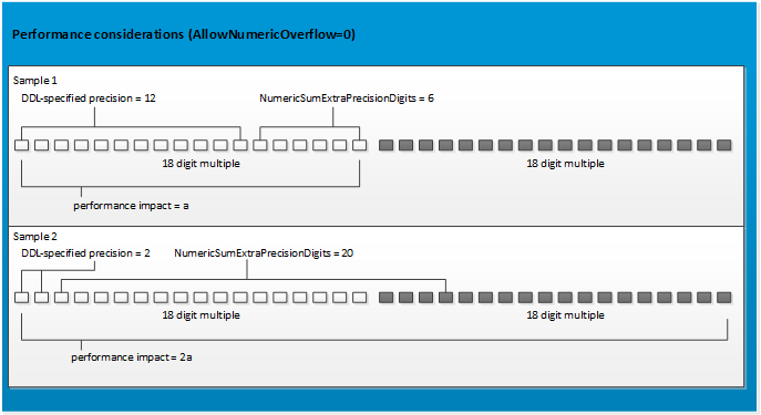
Tip
Vertica recommends that you turn off silent numeric overflow and set the parameter NumericSumExtraPrecisionDigits if you expect query results to exceed the precision specified in the DDL of numeric columns. Be aware of the following considerations:
- If you turn off AllowNumericOverflow and exceed the number of extra precision digits set by NumericSumExtraPrecisionDigits, Vertica returns an error.
- Be careful to set NumericSumExtraPrecisionDigits only as high as necessary to return the SUM of numeric columns.
Impact on pre-aggregated data projections
Vertica supports silent numeric overflow for queries that use SUM or SUM_FLOAT on projections with pre-aggregated data such as live aggregate or Top-K projections. To turn off silent numeric overflow for these queries:
-
Set AllowNumericOverflow to 0.
-
Set NumericSumExtraPrecisionDigits to the desired number of implicit digits. Alternatively, use the default setting of 6.
-
Drop and re-create the affected projections.
If you turn off silent numeric overflow, be aware that overflow can sometimes cause rollback or errors:
-
Overflow occurs during load operations, such as COPY, MERGE, or INSERT:
Vertica aggregates data before loading the projection with data. If overflow occurs while data is aggregated, , Vertica rolls back the load operation.
-
Overflow occurs after load, while Vertica sums existing data.
Vertica computes the sum of existing data separately from the computation that it does during data load. If the projection selects a column with SUM or SUM_FLOAT and overflow occurs, Vertica produces an error message. This response resembles the way Vertica produces an error for a query that uses SUM or SUM_FLOAT.
-
Overflow occurs during mergeout.
Vertica logs a message during mergeout if overflow occurs while Vertica computes a final sum during the mergeout operation. If an error occurs, Vertica marks the projection as out of date and disqualifies it from further mergeout operations.
7 - Spatial data types
The maximum amount of spatial data that a GEOMETRY or GEOGRAPHY column can store, up to 10 MB.
Vertica supports two spatial data types. These data types store two- and three-dimensional spatial objects in a table column:
The maximum size of a GEOMETRY or GEOGRAPHY data type is 10,000,000 bytes (10 MB). You cannot use either data type as a table's primary key.
Syntax
GEOMETRY [ (length) ]
GEOGRAPHY [ (length) ]
Parameters
length- The maximum amount of spatial data that a
GEOMETRY or GEOGRAPHY column can store, up to 10 MB.
Default: 1 MB
8 - UUID data type
Stores universally unique identifiers (UUIDs).
Stores universally unique identifiers (UUIDs). UUIDs are 16-byte (128-bit) numbers used to uniquely identify records. To generate UUIDs, Vertica provides the function
UUID_GENERATE, which returns UUIDs based on high-quality randomness from /dev/urandom.
Syntax
UUID
UUIDs support input of case-insensitive string literal formats, as specified by RFC 4122. In general, a UUID is written as a sequence of hexadecimal digits, in several groups optionally separated by hyphens, for a total of 32 digits representing 128 bits.
The following input formats are valid:
6bbf0744-74b4-46b9-bb05-53905d4538e7
{6bbf0744-74b4-46b9-bb05-53905d4538e7}
6BBF074474B446B9BB0553905D4538E7
6BBf-0744-74B4-46B9-BB05-5390-5D45-38E7
On output, Vertica always uses the following format:
xxxxxxxx-xxxx-xxxx-xxxx-xxxxxxxxxxxx
For example, the following table defines column cust_id as a UUID:
=> CREATE TABLE public.Customers
(
    cust_id uuid,
    lname varchar(36),
    fname varchar(24)
);
The following input for cust_id uses several valid formats:
=>  COPY Customers FROM STDIN;
Enter data to be copied followed by a newline.
End with a backslash and a period on a line by itself.
>> {cede66b7-3d29-4da6-b700-871fc0ac57be}|Kearney|Thomas
>> 34462732ed5649838f3be735b0c32d50|Pham|Duc
>> 9fb0-1de0-1d63-4d09-9415-90e0-b4e9-3b9a|Steinberg|Jeremy
>> \.
On querying this table, Vertica formats all cust_id data in the same way:
=> SELECT cust_id, fname, lname FROM Customers;
                cust_id                | fname  |   lname
--------------------------------------+--------+-----------
 9fb01de0-1d63-4d09-9415-90e0b4e93b9a | Jeremy | Steinberg
 34462732-ed56-4983-8f3b-e735b0c32d50 | Duc    | Pham
 cede66b7-3d29-4da6-b700-871fc0ac57be | Thomas | Kearney
(3 rows)
Generating UUIDs
You can use the Vertica function
UUID_GENERATE to automatically generate UUIDs that uniquely identify table records. For example:
=> INSERT INTO Customers SELECT UUID_GENERATE(),'Rostova','Natasha';
 OUTPUT
--------
      1
(1 row)

=> COMMIT;
COMMIT
=> SELECT cust_id, fname, lname FROM Customers;
               cust_id                |  fname  |   lname
--------------------------------------+---------+-----------
 9fb01de0-1d63-4d09-9415-90e0b4e93b9a | Jeremy  | Steinberg
 34462732-ed56-4983-8f3b-e735b0c32d50 | Duc     | Pham
 cede66b7-3d29-4da6-b700-871fc0ac57be | Thomas  | Kearney
 9aad6757-fe1b-473a-a109-b89b7b358c69 | Natasha | Rostova
(4 rows)
The following string is reserved as NULL for UUID columns:
00000000-0000-0000-0000-000000000000
Vertica always renders NULL as blank.
The following COPY statements insert NULL values into the UUID column, explicitly and implicitly:
=>  COPY Customers FROM STDIN NULL AS 'null';
Enter data to be copied followed by a newline.
End with a backslash and a period on a line by itself.
>> null|Doe|Jane
>> 00000000-0000-0000-0000-000000000000|Man|Nowhere
>> \.
=>  COPY Customers FROM STDIN;
>> |Doe|John
>> \.
In all cases, Vertica renders NULL as blank:
=> SELECT cust_id, fname, lname FROM Customers WHERE cust_id IS NULL;
 cust_id |  fname  | lname
---------+---------+-------
         | Nowhere | Man
         | Jane    | Doe
         | John    | Doe
(3 rows)
Usage restrictions
UUID data types only support relational operators and functions that are also supported by CHAR and VARCHAR data types—for example,
MIN,
MAX, and
COUNT. UUID data types do not support mathematical operators or functions, such as
SUM and
AVG.
9 - Data type coercion
Vertica supports two types of data type casting:.
Vertica supports two types of data type casting:
Implicit casting
The ANSI SQL-92 standard supports implicit casting among similar data types:
-
Number types
-
CHAR, VARCHAR, LONG VARCHAR
-
BINARY, VARBINARY, LONG VARBINARY
Vertica supports two types of nonstandard implicit casts of scalar types:
-
From CHAR to FLOAT, to match the one from VARCHAR to FLOAT. The following example converts the CHAR '3' to a FLOAT so it can add the number 4.33 to the FLOAT result of the second expression:
=> SELECT '3'::CHAR + 4.33::FLOAT;
 ?column?
----------
   7.33
(1 row)
-
Between DATE and TIMESTAMP. The following example DATE to a TIMESTAMP and calculates the time 6 hours, 6 minutes, and 6 seconds back from 12:00 AM:
=> SELECT DATE('now') - INTERVAL '6:6:6';
      ?column?
---------------------
 2013-07-30 17:53:54
(1 row)
When there is no ambiguity about the data type of an expression value, it is implicitly coerced to match the expected data type. In the following statement, the quoted string constant '2' is implicitly coerced into an INTEGER value so that it can be the operand of an arithmetic operator (addition):
=> SELECT 2 + '2';
 ?column?
----------
        4
(1 row)
A concatenate operation explicitly takes arguments of any data type. In the following example, the concatenate operation implicitly coerces the arithmetic expression 2 + 2 and the INTEGER constant 2 to VARCHAR values so that they can be concatenated.
=> SELECT 2 + 2 || 2;
 ?column?
----------
 42
(1 row)
Another example is to first get today's date:
=> SELECT DATE 'now';
  ?column?
------------
 2013-07-31
(1 row)
The following command converts DATE to a TIMESTAMP and adds a day and a half to the results by using INTERVAL:
=> SELECT DATE 'now' + INTERVAL '1 12:00:00';
      ?column?
---------------------
 2013-07-31 12:00:00
(1 row)
Most implicit casts stay within their relational family and go in one direction, from less detailed to more detailed. For example:
-
DATE to TIMESTAMP/TZ
-
INTEGER to NUMERIC to FLOAT
-
CHAR to FLOAT
-
CHAR to VARCHAR
-
CHAR and/or VARCHAR to FLOAT
-
CHAR to LONG VARCHAR
-
VARCHAR to LONG VARCHAR
-
BINARY to VARBINARY
-
BINARY to LONG VARBINARY
-
VARBINARY to LONG VARBINARY
More specifically, data type coercion works in this manner in Vertica:
|
Conversion |
Notes |
|
INT8 > FLOAT8 |
Implicit, can lose significance |
|
FLOAT8 > INT8 |
Explicit, rounds |
|
VARCHAR <-> CHAR |
Implicit, adjusts trailing spaces |
|
VARBINARY <-> BINARY |
Implicit, adjusts trailing NULs |
|
VARCHAR > LONG VARCHAR |
Implicit, adjusts trailing spaces |
|
VARBINARY > LONG VARBINARY |
Implicit, adjusts trailing NULs |
No other types cast to or from LONGVARBINARY, VARBINARY, or BINARY. In the following list, <any> means one these types: INT8, FLOAT8, DATE, TIME, TIMETZ, TIMESTAMP, TIMESTAMPTZ, INTERVAL:
-
<any> -> VARCHAR—implicit
-
VARCHAR -> <any>—explicit, except that VARCHAR->FLOAT is implicit
-
<any> <-> CHAR—explicit
-
DATE -> TIMESTAMP/TZ—implicit
-
TIMESTAMP/TZ -> DATE—explicit, loses time-of-day
-
TIME -> TIMETZ—implicit, adds local timezone
-
TIMETZ -> TIME—explicit, loses timezone
-
TIME -> INTERVAL—implicit, day to second with days=0
-
INTERVAL -> TIME—explicit, truncates non-time parts
-
TIMESTAMP <-> TIMESTAMPTZ—implicit, adjusts to local timezone
-
TIMESTAMP/TZ -> TIME—explicit, truncates non-time parts
-
TIMESTAMPTZ -> TIMETZ—explicit
-
VARBINARY -> LONG VARBINARY—implicit
-
LONG VARBINARY -> VARBINARY—explicit
-
VARCHAR -> LONG VARCHAR—implicit
-
LONG VARCHAR -> VARCHAR—explicit
Important
Implicit casts from INTEGER, FLOAT, and NUMERIC to VARCHAR are not supported. If you need that functionality, write an explicit cast:
CAST(x AS data-type-name)
or
x::data-type-name
The following example casts a FLOAT to an INTEGER:
=> SELECT(FLOAT '123.5')::INT;
 ?column?
----------
      124
(1 row)
String-to-numeric data type conversions accept formats of quoted constants for scientific notation, binary scaling, hexadecimal, and combinations of numeric-type literals:
-
Scientific notation:
=> SELECT FLOAT '1e10';
  ?column?
-------------
 10000000000
(1 row)
-
BINARY scaling:
=> SELECT NUMERIC '1p10';
 ?column?
----------
     1024
(1 row)
-
hexadecimal:
=> SELECT NUMERIC '0x0abc';
 ?column?
----------
     2748
(1 row)
Complex types
Collections (arrays and sets) can be cast implicitly and explicitly. Casting a collection casts each element of the collection. You can, for example, cast an ARRAY[VARCHAR] to an ARRAY[INT] or a SET[DATE] to SET[TIMESTAMPTZ]. You can cast between arrays and sets.
When casting to a bounded native array, inputs that are too long are truncated. When casting to a non-native array (an array containing complex data types including other arrays), if the new bounds are too small for the data the cast fails
Rows (structs) can be cast implicitly and explicitly. Casting a ROW casts each field value. You can specify new field names in the cast or specify only the field types to use the existing field names.
Casting can increase the storage needed for a column. For example, if you cast an array of INT to an array of VARCHAR(50), each element takes more space and thus the array takes more space. If the difference is extreme or the array has many elements, this could mean that the array no longer fits within the space allotted for the column. In this case the operation reports an error and fails.
Examples
The following example casts three strings as NUMERICs:
=> SELECT NUMERIC '12.3e3', '12.3p10'::NUMERIC, CAST('0x12.3p-10e3' AS NUMERIC);
 ?column? | ?column? |     ?column?
----------+----------+-------------------
    12300 |  12595.2 | 17.76123046875000
(1 row)
This example casts a VARBINARY string into a LONG VARBINARY data type:
=> SELECT B'101111000'::LONG VARBINARY;
 ?column?
----------
 \001x
(1 row)
The following example concatenates a CHAR with a LONG VARCHAR, resulting in a LONG VARCHAR:
=> \set s ''''`cat longfile.txt`''''
=> SELECT length ('a' || :s ::LONG VARCHAR);
 length
----------
 65002
(1 row)
The following example casts a combination of NUMERIC and INTEGER data into a NUMERIC result:
=> SELECT (18. + 3./16)/1024*1000;
                ?column?
-----------------------------------------
 17.761230468750000000000000000000000000
(1 row)
Note
In SQL expressions, pure numbers between (–2^63–1) and (2^63–1) are INTEGERs. Numbers with decimal points are NUMERIC.
See also
10 - Data type coercion chart
The following table defines all possible type conversions that Vertica supports.
Conversion types
The following table defines all possible type conversions that Vertica supports. The data types in the first column of the table are the inputs to convert, and the remaining columns indicate the result for the different conversion types.
|
Source Data Type |
Implicit |
Explicit |
Assignment |
Assignment without numeric meaning |
Conversion without explicit casting |
|
BOOLEAN |
|
|
INTEGER, LONG VARCHAR, VARCHAR, CHAR |
|
|
|
INTEGER |
BOOLEAN, NUMERIC, FLOAT |
|
INTERVAL DAY/SECOND, INTERVAL YEAR/MONTH |
LONG VARCHAR, VARCHAR, CHAR |
|
|
NUMERIC |
FLOAT |
|
INTEGER |
LONG VARCHAR, VARCHAR, CHAR |
NUMERIC |
|
FLOAT |
|
|
INTEGER, NUMERIC |
LONG VARCHAR, VARCHAR, CHAR |
|
|
LONG VARCHAR |
FLOAT, CHAR |
BOOLEAN, INTEGER, NUMERIC, VARCHAR, TIMESTAMP, TIMESTAMPTZ, DATE, TIME, TIMETZ, INTERVAL DAY/SECOND, INTERVAL YEAR/MONTH, LONG VARBINARY |
|
|
LONG VARCHAR |
|
VARCHAR |
CHAR, FLOAT, LONG VARCHAR |
BOOLEAN, INTEGER, NUMERIC, TIMESTAMP, TIMESTAMPTZ, DATE, TIME, TIMETZ, UUID, BINARY, VARBINARY, INTERVAL DAY/SECOND, INTERVAL YEAR/MONTH |
|
|
VARCHAR |
|
CHAR |
FLOAT, LONG VARCHAR, VARCHAR |
BOOLEAN, INTEGER, NUMERIC, TIMESTAMP, TIMESTAMPTZ, DATE, TIME, TIMETZ, UUID (CHAR length ≥ 36), BINARY, VARBINARY, INTERVAL DAY/SECOND, INTERVAL YEAR/MONTH |
|
|
CHAR |
|
TIMESTAMP |
TIMESTAMPTZ |
|
LONG CHAR, VARCHAR, CHAR, DATE, TIME |
|
TIMESTAMP |
|
TIMESTAMPTZ |
TIMESTAMP |
|
LONG CHAR, VARCHAR, CHAR, DATE, TIME, TIMETZ |
|
TIMESTAMPTZ |
|
DATE |
TIMESTAMP |
|
LONG CHAR, VARCHAR, CHAR, TIMESTAMPTZ |
|
|
|
TIME |
TIMETZ |
TIMESTAMP, TIMESTAMPTZ, INTERVAL DAY/SECOND |
LONG CHAR, VARCHAR, CHAR |
|
TIME |
|
TIMETZ |
|
TIMESTAMP, TIMESTAMPTZ |
LONG CHAR, VARCHAR, CHAR, TIME |
|
TIMETZ |
|
INTERVAL DAY/SECOND |
|
TIME |
INTEGER, LONG CHAR, VARCHAR, CHAR |
|
INTERVAL DAY/SECOND |
|
INTERVAL YEAR/MONTH |
|
|
INTEGER, LONG CHAR, VARCHAR, CHAR |
|
INTERVAL YEAR/MONTH |
|
LONG VARBINARY |
|
VARBINARY |
|
|
LONG VARBINARY |
|
VARBINARY |
LONG VARBINARY, BINARY |
|
|
|
VARBINARY |
|
BINARY |
VARBINARY |
|
|
|
BINARY |
|
UUID |
|
CHAR(36), VARCHAR |
|
|
UUID |
Implicit and explicit conversion
Vertica supports data type conversion of values without explicit casting, such as NUMERIC(10,6) -> NUMERIC(18,4).Implicit data type conversion occurs automatically when converting values of different, but compatible, types to the target column's data type. For example, when adding values, (INTEGER + NUMERIC), the result is implicitly cast to a NUMERIC type to accommodate the prominent type in the statement. Depending on the input data types, different precision and scale can occur.
An explicit type conversion must occur when the source data cannot be cast implicitly to the target column's data type.
Assignment conversion
In data assignment conversion, coercion implicitly occurs when values are assigned to database columns in an INSERT or UPDATE...SET statement. For example, in a statement that includes INSERT...VALUES('2.5'), where the target column data type is NUMERIC(18,5), a cast from VARCHAR to the column data type is inferred.
In an assignment without numeric meaning, the value is subject to CHAR/VARCHAR/LONG VARCHAR comparisons.
See also
11 - Complex types
Complex types such as structures (also known as rows), arrays, and maps are composed of primitive types and sometimes other complex types.
Complex types such as structures (also known as rows), arrays, and maps are composed of primitive types and sometimes other complex types. Complex types can be used in the following ways:
-
Arrays and rows (in any combination) can be used as column data types in both native and external tables.
-
Sets of primitive element types can be used as column data types in native and external tables.
-
Arrays and rows, but not combinations of them, can be created as literals, for example to use in query expressions.
The MAP type is a legacy type. To represent maps, use ARRAY[ROW].
If a flex table has a real column that uses a complex type, the values from that column are not included in the __raw__ column. For more information, see Loading Data into Flex Table Real Columns.
11.1 - ARRAY
Represents array data.
Represents array data. There are two types of arrays in Vertica:
-
Native array: a one-dimensional array of a primitive type. Native arrays are tracked in the TYPES system table and used in native tables.
-
Non-native array: all other supported arrays, including arrays that contain other arrays (multi-dimensional arrays) or structs (ROWs). Non-native arrays have some usage restrictions. Non-native arrays are tracked in the COMPLEX_TYPES system table.
Both types of arrays operate in the same way, but they have different OIDs.
Arrays can be bounded, meaning they specify a maximum element count, or unbounded. Unbounded arrays have a maximum binary size, which can be set explicitly or defaulted. See Limits on Element Count and Collection Size.
Selected parsers support using COPY to load arrays. See the documentation of individual parsers for more information.
Syntax
In column definitions:
ARRAY[data_type, max_elements] |
ARRAY[data_type](max_size) |
ARRAY[data_type]
In literals:
ARRAY[value[, ...] ]
Restrictions
-
Native arrays support only data of primitive types, for example, int, UUID, and so on.
-
Array dimensionality is enforced. A column cannot contain arrays of varying dimensions. For example, a column that contains a three-dimensional array can only contain other three-dimensional arrays; it cannot simultaneously include a one-dimensional array. However, the arrays in a column can vary in size, where one array can contain four elements while another contains ten.
-
Array bounds, if specified, are enforced for all operations that load or alter data. Unbounded arrays may have as many elements as will fit in the allotted binary size.
-
An array has a maximum binary size. If this size is not set when the array is defined, a default value is used.
-
Arrays do not support LONG types (like LONG VARBINARY or LONG VARCHAR) or user-defined types (like Geometry).
Syntax for column definition
Arrays used in column definitions can be either bounded or unbounded. Bounded arrays must specify a maximum number of elements. Unbounded arrays can specify a maximum binary size (in bytes) for the array, or the value of DefaultArrayBinarySize is used. You can specify a bound or a binary size but not both. For more information about these values, see Limits on Element Count and Collection Size.
|
Type |
Syntax |
Semantics |
|
Bounded array |
ARRAY[data_type, max_elements]
Example:
ARRAY[VARCHAR(50),100]
|
Can contain no more than max_elements elements. Attempting to add more is an error.
Has a binary size of the size of the data type multiplied by the maximum number of elements (possibly rounded up).
|
|
Unbounded array with maximum binary size |
ARRAY[data_type](max_size)
Example:
ARRAY[VARCHAR(50)](32000)
|
Can contain as many elements as fit in max_size. Ignores the value of DefaultArrayBinarySize. |
|
Unbounded array with default binary size |
ARRAY[data_type]
Example:
ARRAY[VARCHAR(50)]
|
Can contain as many elements as fit in the default binary size.
Equivalent to:
ARRAY[data_type](DefaultArrayBinarySize)
|
The following example defines a table for customers using an unbounded array:
=> CREATE TABLE customers (id INT, name VARCHAR, email ARRAY[VARCHAR(50)]);
The following example uses a bounded array for customer email addresses and an unbounded array for order history:
=> CREATE TABLE customers (id INT, name VARCHAR, email ARRAY[VARCHAR(50),5], orders ARRAY[INT]);
The following example uses an array that has ROW elements:
=> CREATE TABLE orders(
  orderid INT,
  accountid INT,
  shipments ARRAY[
    ROW(
      shipid INT,
      address ROW(
        street VARCHAR,
        city VARCHAR,
        zip INT
        ),
      shipdate DATE
    )
  ]
 );
To declare a multi-dimensional array, use nesting. For example, ARRAY[ARRAY[int]] specifies a two-dimensional array.
Syntax for direct construction (literals)
Use the ARRAY keyword to construct an array value. The following example creates an array of integer values.
=> SELECT ARRAY[1,2,3];
 array
-------
 [1,2,3]
(1 row)
You can nest an array inside another array, as in the following example.
=> SELECT ARRAY[ARRAY[1],ARRAY[2]];
   array
-----------
 [[1],[2]]
(1 row)
If an array of arrays contains no null elements and no function calls, you can abbreviate the syntax:
=> SELECT ARRAY[[1,2],[3,4]];
     array
---------------
 [[1,2],[3,4]]
(1 row)

---not valid:
=> SELECT ARRAY[[1,2],null,[3,4]];

ERROR 4856:  Syntax error at or near "null" at character 20
LINE 1: SELECT ARRAY[[1,2],null,[3,4]];
                           ^
Array literals can contain elements of all scalar types, ROW, and ARRAY. ROW elements must all have the same set of fields:
=> SELECT ARRAY[ROW(1,2),ROW(1,3)];
               array
-----------------------------------
 [{"f0":1,"f1":2},{"f0":1,"f1":3}]
(1 row)

=> SELECT ARRAY[ROW(1,2),ROW(1,3,'abc')];
ERROR 3429:  For 'ARRAY', types ROW(int,int) and ROW(int,int,unknown) are inconsistent
Because the elements are known at the time you directly construct an array, these arrays are implicitly bounded.
You can use ARRAY literals in comparisons, as in the following example:
=> SELECT id.name, id.num, GPA FROM students
   WHERE major = ARRAY[ROW('Science','Physics')];
 name  | num | GPA
-------+-----+-----
 bob   | 121 | 3.3
 carol | 123 | 3.4
(2 rows)
Queries of array columns return JSON format, with the values shown in comma-separated lists in brackets. The following example shows a query that includes array columns.
=> SELECT cust_custkey,cust_custstaddress,cust_custcity,cust_custstate from cust;
cust_custkey |               cust_custstaddress                      |                cust_custcity                | cust_custstate
-------------+-------  ----------------------------------------------+---------------------------------------------+----------------
      342176 | ["668 SW New Lane","518 Main Ave","7040 Campfire Dr"] | ["Winchester","New Hyde Park","Massapequa"] | ["VA","NY","NY"]
      342799 | ["2400 Hearst Avenue","3 Cypress Street"]             | ["Berkeley","San Antonio"]                  | ["CA","TX"]
      342845 | ["336 Boylston Street","180 Clarkhill Rd"]            | ["Boston","Amherst"]                        | ["MA","MA"]
      342321 | ["95 Fawn Drive"]                                     | ["Allen Park"]                              | ["MI"]
      342989 | ["5 Thompson St"]                                     | ["Massillon"]                               | ["OH"]
(5 rows)
Note that JSON format escapes some characters that would not be escaped in native VARCHARs. For example, if you insert "c:\users\data" into an array, the JSON output for that value is "c:\\users\\data".
Element access
Arrays are 0-indexed. The first element's ordinal position is 0, second is 1, and so on.
You can access (dereference) elements from an array by index:
=> SELECT (ARRAY['a','b','c','d','e'])[1];
array
-------
b
(1 row)
To specify a range, use the format start:end. The end of the range is non-inclusive.
=> SELECT(ARRAY['a','b','c','d','e','f','g'])[1:4];
array
---------
["b","c","d"]
(1 row)
To dereference an element from a multi-dimensional array, put each index in brackets:
=> SELECT(ARRAY[ARRAY[1,2],ARRAY[3,4]])[0][0];
 array
-------
 1
(1 row)
Out-of-bound index references return NULL.
Limits on element count and collection size
When declaring a collection type for a table column, you can limit either the number of elements or the total binary size of the collection. During query processing, Vertica always reserves the maximum memory needed for the column, based on either the element count or the binary size. If this size is much larger than your data actually requires, setting one of these limits can improve query performance by reducing the amount of memory that must be reserved for the column.
You can change the bounds of a collection, including changing between bounded and unbounded collections, by casting. See Casting.
A bounded collection specifies a maximum element count. A value in a bounded collection column may contain fewer elements, but it may not contain more. Any attempt to insert more elements into a bounded collection than the declared maximum is an error. A bounded collection has a binary size that is the product of the data-type size and the maximum number of elements, possibly rounded up.
An unbounded collection specifies a binary size in bytes, explicitly or implicitly. It may contain as many elements as can fit in that binary size.
If a nested array specifies bounds for all dimensions, Vertica sets a single bound that is the product of the bounds. In the following example, the inner and outer arrays each have a bound of 10, but only a total element count of 100 is enforced.
ARRAY[ARRAY[INT,10],10]
If a nested array specifies a bound for only the outer collection, it is treated as the total bound. The previous example is equivalent to the following:
ARRAY[ARRAY[INT],100]
You must either specify bounds for all nested collections or specify a bound only for the outer one. For any other distribution of bounds, Vertica treats the collection as unbounded.
Instead of specifying a bound, you can specify a maximum binary size for an unbounded collection. The binary size acts as an absolute limit, regardless of how many elements the collection contains. Collections that do not specify a maximum binary size use the value of DefaultArrayBinarySize. This size is set at the time the collection is defined and is not affected by later changes to the value of DefaultArrayBinarySize.
You cannot set a maximum binary size for a bounded collection, only an unbounded one.
You can change the bounds or the binary size of an array column using ALTER TABLE as in the following example:
=> ALTER TABLE cust ALTER COLUMN orders SET DATA TYPE ARRAY[INTEGER](100);
If the change reduces the size of the collection and would result in data loss, the change fails.
Comparisons
All collections support equality (=), inequality (<>), and null-safe equality (<=>). 1D collections also support comparison operators (<, <=, >, >=) between collections of the same type (arrays or sets). Comparisons follow these rules:
-
A null collection is ordered last.
-
Non-null collections are compared element by element, using the ordering rules of the element's data type. The relative order of the first pair of non-equal elements determines the order of the two collections.
-
If all elements in both collections are equal up to the length of the shorter collection, the shorter collection is ordered before the longer one.
-
If all elements in both collections are equal and the collections are of equal length, the collections are equal.
Null-handling
Null semantics for collections are consistent with normal columns in most regards. See NULL sort order for more information on null-handling.
The null-safe equality operator (<=>) behaves differently from equality (=) when the collection is null rather than empty. Comparing a collection to NULL strictly returns null:
=> SELECT ARRAY[1,3] = NULL;
?column?
----------

(1 row)

=> SELECT ARRAY[1,3] <=> NULL;
 ?column?
----------
 f
(1 row)
In the following example, the grants column in the table is null for employee 99:
=> SELECT grants = NULL FROM employees WHERE id=99;
 ?column?
----------

(1 row)

=> SELECT grants <=> NULL FROM employees WHERE id=99;
 ?column?
----------
 t
(1 row)
Empty collections are not null and behave as expected:
=> SELECT ARRAY[]::ARRAY[INT] = ARRAY[]::ARRAY[INT];
 ?column?
----------
 t
(1 row)
Collections are compared element by element. If a comparison depends on a null element, the result is unknown (null), not false. For example, ARRAY[1,2,null]=ARRAY[1,2,null] and ARRAY[1,2,null]=ARRAY[1,2,3] both return null, but ARRAY[1,2,null]=ARRAY[1,4,null] returns false because the second elements do not match.
Casting
Casting an array casts each element of the array. You can therefore cast between data types following the same rules as for casts of scalar values.
You can cast both literal arrays and array columns explicitly:
=> SELECT ARRAY['1','2','3']::ARRAY[INT];
  array
---------
[1,2,3]
(1 row)
You can change the bound of an array or set by casting. When casting to a bounded native array, inputs that are too long are truncated. When casting to a non-native array (an array containing complex data types including other arrays), if the new bounds are too small for the data the cast fails:
=> SELECT ARRAY[1,2,3]::ARRAY[VARCHAR,2];
   array
-----------
 ["1","2"]
(1 row)

=> SELECT ARRAY[ARRAY[1,2,3],ARRAY[4,5,6]]::ARRAY[ARRAY[VARCHAR,2],2];
ERROR 9227:  Output array isn't big enough
DETAIL:  Type limit is 4 elements, but value has 6 elements
If you cast to a bounded multi-dimensional array, you must specify the bounds at all levels:
=> SELECT ARRAY[ARRAY[1,2,3],ARRAY[4,5,6]]::ARRAY[ARRAY[VARCHAR,5],10];
             array
-------------------------------
 [["1","2","3"],["4","5","6"]]
(1 row)

=> SELECT ARRAY[ARRAY[1,2,3],ARRAY[4,5,6]]::ARRAY[ARRAY[VARCHAR,2]];
WARNING 9753:  Collection type bound will not be used
DETAIL:  A bound was provided for an inner dimension, but not for an outer dimension
             array
-------------------------------
 [["1","2","3"],["4","5","6"]]
(1 row)
Assignment casts and implicit casts work the same way as for scalars:
=> CREATE TABLE transactions (tid INT, prod_ids ARRAY[VARCHAR,100], quantities ARRAY[INT,100]);
CREATE TABLE

=> INSERT INTO transactions VALUES (12345, ARRAY['p1265', 'p4515'], ARRAY[15,2]);
 OUTPUT
--------
      1
(1 row)

=> CREATE TABLE txreport (prod_ids ARRAY[VARCHAR(12),100], quants ARRAY[VARCHAR(32),100]);
CREATE TABLE

=> INSERT INTO txreport SELECT prod_ids, quantities FROM transactions;
 OUTPUT
--------
      1
(1 row)

=> SELECT * FROM txreport;
     prod_ids      |   quants
-------------------+------------
 ["p1265","p4515"] | ["15","2"]
(1 row)
You can perform explicit casts, but not implicit casts, between the ARRAY and SET types (native arrays only). If the collection is unbounded and the data type does not change, the binary size is preserved. For example, if you cast an ARRAY[INT] to a SET[INT], the set has the same binary size as the array.
If you cast from one element type to another, the resulting collection uses the default binary size. If this would cause the data not to fit, the cast fails.
You cannot cast from an array to an array with a different dimensionality, for example from a two-dimensional array to a one-dimensional array.
Functions and operators
See Collection functions for a comprehensive list of functions that can be used to manipulate arrays and sets.
Collections can be used in the following ways:
Collections cannot be used in the following ways:
-
As part of an IN or NOT IN expression.
-
As partition columns when creating tables.
-
With ANALYZE_STATISTICS or TopK projections.
-
Non-native arrays only: ORDER BY, PARTITION BY, DEFAULT, SET USING, or constraints.
11.2 - MAP
Represents map data in external tables in the Parquet, ORC, and Avro formats only.
Represents map data in external tables in the Parquet, ORC, and Avro formats only. A MAP must use only primitive types and may not contain other complex types. You can use the MAP type in a table definition to consume columns in the data, but you cannot query those columns.
A superior alternative to MAP is ARRAY[ROW]. An array of rows can use all supported complex types and can be queried. This is the representation that INFER_TABLE_DDL suggests. For Avro data, the ROW must have fields named key and value.
Within a single table you must define all map columns using the same approach, MAP or ARRAY[ROW].
Syntax
In column definitions:
MAP<key,value>
In a column definition in an external table, a MAP consists of a key-value pair, specified as types. The table in the following example defines a map of product IDs to names.
=> CREATE EXTERNAL TABLE store (storeID INT, inventory MAP<INT,VARCHAR(100)>)
    AS COPY FROM '...' PARQUET;
11.3 - ROW
Represents structured data (structs).
Represents structured data (structs). A ROW can contain fields of any primitive or complex type supported by Vertica.
Syntax
In column definitions:
ROW([field] type[, ...])
If the field name is omitted, Vertica generates names starting with "f0".
In literals:
ROW(value [AS field] [, ...]) [AS name(field[, ...])]
Syntax for column definition
In a column definition, a ROW consists of one or more comma-separated pairs of field names and types. In the following example, the Parquet data file contains a struct for the address, which is read as a ROW in an external table:
=> CREATE EXTERNAL TABLE customers (name VARCHAR,
    address ROW(street VARCHAR, city VARCHAR, zipcode INT))
    AS COPY FROM '...' PARQUET;
ROWs can be nested; a field can have a type of ROW:
=> CREATE TABLE employees(
    employeeID INT,
    personal ROW(
      name VARCHAR,
      address ROW(street VARCHAR, city VARCHAR, zipcode INT),
      taxID INT),
    department VARCHAR);
ROWs can contain arrays:
=> CREATE TABLE customers(
  name VARCHAR,
  contact ROW(
    street VARCHAR,
    city VARCHAR,
    zipcode INT,
    email ARRAY[VARCHAR]
  ),
  accountid INT );
When loading data, the primitive types in the table definition must match those in the data. The ROW structure must also match; a ROW must contain all and only the fields in the struct in the data.
Restrictions on ROW columns
ROW columns have several restrictions:
- Maximum nesting depth is 100.
- Vertica tables support up to 9800 columns and fields. The ROW itself is not counted, only its fields.
- ROW columns cannot use any constraints (such as NOT NULL) or defaults.
- ROW fields cannot be auto_increment or setof.
- ROW definition must include at least one field.
Row is a reserved keyword within a ROW definition, but is permitted as the name of a table or column.- Tables containing ROW columns cannot also contain IDENTITY, default, SET USING, or named sequence columns.
Syntax for direct construction (literals)
In a literal, such as a value in a comparison operation, a ROW consists of one or more values. If you omit field names in the ROW expression, Vertica generates them automatically. If you do not coerce types, Vertica infers the types from the data values.
=> SELECT ROW('Amy',2,false);
                row
--------------------------------------------
 {"f0":"Amy","f1":2,"f2":false}
(1 row)
You can use an AS clause to name the ROW and its fields:
=> SELECT ROW('Amy',2,false) AS student(name, id, current);
               student
--------------------------------------------
 {"name":"Amy","id":2,"current":false}
(1 row)
You can also name individual fields using AS. This query produces the same output as the previous one:
=> SELECT ROW('Amy' AS name, 2 AS id, false AS current) AS student;
You do not need to name all fields.
In an array of ROW elements, if you use AS to name fields and the names differ among the elements, Vertica uses the right-most names for all elements:
=> SELECT ARRAY[ROW('Amy' AS name, 2 AS id),ROW('Fred' AS first_name, 4 AS id)];
                           array
------------------------------------------------------------
 [{"first_name":"Amy","id":2},{"first_name":"Fred","id":4}]
(1 row)
You can coerce types explicitly:
=> SELECT ROW('Amy',2.5::int,false::varchar);
               row
------------------------------------------
 {"f0":"Amy","f1":3,"f2":"f"}
(1 row)
Escape single quotes in literal inputs using single quotes, as in the following example:
=> SELECT ROW('Howard''s house',2,false);
                      row
---------------------------------------------------
 {"f0":"Howard's house","f1":2,"f2":false}
(1 row)
You can use fields of all scalar types, ROW, and ARRAY, as in the following example:
=> SELECT id.name, major, GPA FROM students
   WHERE id = ROW('alice',119, ARRAY['alice@example.com','ap16@cs.example.edu']);
 name  |               major                | GPA
-------+------------------------------------+-----
 alice | [{"school":"Science","dept":"CS"}] | 3.8
(1 row)
ROW values are output in JSON format as in the following example.
=> CREATE EXTERNAL TABLE customers (name VARCHAR,
    address ROW(street VARCHAR, city VARCHAR, zipcode INT))
    AS COPY FROM '...' PARQUET;

=> SELECT address FROM customers WHERE address.city ='Pasadena';
                              address
--------------------------------------------------------------------
 {"street":"100 Main St Apt 4B","city":"Pasadena","zipcode":91001}
 {"street":"100 Main St Apt 4A","city":"Pasadena","zipcode":91001}
 {"street":"23 Fifth Ave Apt 8C","city":"Pasadena","zipcode":91001}
 {"street":"15 Raymond Dr","city":"Pasadena","zipcode":91003}
(4 rows)
The following table specifies the mappings from Vertica data types to JSON data types.
|
Vertica Type |
JSON Type |
|
Integer |
Integer |
|
Float |
Numeric |
|
Numeric |
Numeric |
|
Boolean |
Boolean |
|
All others |
String |
Comparisons
ROW supports equality (=), inequality (<>), and null-safe equality (<=>) between inputs that have the same set of fields. ROWs that contain only primitive types, including nested ROWs of primitive types, also support comparison operators (<, <=, >, >=).
Two ROWs are equal if and only if all fields are equal. Vertica compares fields in order until an inequality is found or all fields have been compared. The evaluation of the first non-equal field determines which ROW is greater:
=> SELECT ROW(1, 'joe') > ROW(2, 'bob');
?column?
----------
f
(1 row)
Comparisons between ROWs with different schemas fail:
=> SELECT ROW(1, 'joe') > ROW(2, 'bob', 123);
ERROR 5162:  Unequal number of entries in row expressions
If the result of a comparison depends on a null field, the result is null:
=>  select row(1, null, 3) = row(1, 2, 3);
 ?column?
----------

(1 row)
Null-handling
If a struct exists but a field value is null, Vertica assigns NULL as its value in the ROW. A struct where all fields are null is treated as a ROW with null fields. If the struct itself is null, Vertica reads the ROW as NULL.
Casting
Casting a ROW casts each field. You can therefore cast between data types following the same rules as for casts of scalar values.
The following example casts the contact ROW in the customers table, changing the zipcode field from INT to VARCHAR and adding a bound to the array:
=> SELECT contact::ROW(VARCHAR,VARCHAR,VARCHAR,ARRAY[VARCHAR,20]) FROM customers;
                                                         contact

--------------------------------------------------------------------------------
-----------------------------------------
 {"street":"911 San Marcos St","city":"Austin","zipcode":"73344","email":["missy@mit.edu","mcooper@cern.gov"]}
 {"street":"100 Main St Apt 4B","city":"Pasadena","zipcode":"91001","email":["shelly@meemaw.name","cooper@caltech.edu"]}
 {"street":"100 Main St Apt 4A","city":"Pasadena","zipcode":"91001","email":["hofstadter@caltech.edu"]}
 {"street":"23 Fifth Ave Apt 8C","city":"Pasadena","zipcode":"91001","email":[]}
 {"street":null,"city":"Pasadena","zipcode":"91001","email":["raj@available.com"]}

(6 rows)
You can specify new field names to change them in the output:
=> SELECT contact::ROW(str VARCHAR, city VARCHAR, zip VARCHAR, email ARRAY[VARCHAR,
20]) FROM customers;
                                                     contact

--------------------------------------------------------------------------------
----------------------------------
 {"str":"911 San Marcos St","city":"Austin","zip":"73344","email":["missy@mit.edu","mcooper@cern.gov"]}
 {"str":"100 Main St Apt 4B","city":"Pasadena","zip":"91001","email":["shelly@meemaw.name","cooper@caltech.edu"]}
 {"str":"100 Main St Apt 4A","city":"Pasadena","zip":"91001","email":["hofstadter@caltech.edu"]}
 {"str":"23 Fifth Ave Apt 8C","city":"Pasadena","zip":"91001","email":[]}
 {"str":null,"city":"Pasadena","zip":"91001","email":["raj@available.com"]}
(6 rows)
Supported operators and predicates
ROW values may be used in queries in the following ways:
-
INNER and OUTER JOIN
-
Comparisons, IN, BETWEEN (non-nullable filters only)
-
IS NULL, IS NOT NULL
-
CASE
-
GROUP BY, ORDER BY
-
SELECT DISTINCT
-
Arguments to user-defined scalar, transform, and analytic functions
The following operators and predicates are not supported for ROW values:
-
Math operators
-
Type coercion of whole rows (coercion of field values is supported)
-
BITWISE, LIKE
-
MLA (ROLLUP, CUBE, GROUPING SETS)
-
Aggregate functions including MAX, MIN, and SUM
-
Set operators including UNION, UNION ALL, MINUS, and INTERSECT
COUNT is not supported for ROWs returned from user-defined scalar functions, but is supported for ROW columns and literals.
In comparison operations (including implicit comparisons like ORDER BY), a ROW literal is treated as the sequence of its field values. For example, the following two statements are equivalent:
GROUP BY ROW(zipcode, city)
GROUP BY zipcode, city
Using rows in views and subqueries
You can use ROW columns to construct views and in subqueries. Consider employee and customer tables with the following definitions:
=> CREATE EXTERNAL TABLE customers(name VARCHAR,
        address ROW(street VARCHAR, city VARCHAR, zipcode INT), accountID INT)
    AS COPY FROM '...' PARQUET;

=> CREATE EXTERNAL TABLE employees(employeeID INT,
        personal ROW(name VARCHAR,
        address ROW(street VARCHAR, city VARCHAR, zipcode INT),
        taxID INT), department VARCHAR)
    AS COPY FROM '...' PARQUET;
The following example creates a view and queries it.
=> CREATE VIEW neighbors (num_neighbors, area(city, zipcode))
AS SELECT count(*), ROW(address.city, address.zipcode)
FROM customers GROUP BY address.city, address.zipcode;
CREATE VIEW

=> SELECT employees.personal.name, neighbors.area FROM neighbors, employees
WHERE employees.personal.address.zipcode=neighbors.area.zipcode AND neighbors.nu
m_neighbors > 1;
        name        |                area
--------------------+-------------------------------------
 Sheldon Cooper     | {"city":"Pasadena","zipcode":91001}
 Leonard Hofstadter | {"city":"Pasadena","zipcode":91001}
(2 rows)
11.4 - SET
Represents a collection of unordered, unique elements.
Represents a collection of unordered, unique elements. Sets may contain only primitive types. In sets, unlike in arrays, element position is not meaningful.
Sets do not support LONG types (like LONG VARBINARY or LONG VARCHAR) or user-defined types (like Geometry).
If you populate a set from an array, Vertica sorts the values and removes duplicate elements. If you do not care about element position and plan to run queries that check for the presence of specific elements (find, contains), using a set could improve query performance.
Sets can be bounded, meaning they specify a maximum element count, or unbounded. Unbounded sets have a maximum binary size, which can be set explicitly or defaulted. See Limits on Element Count and Collection Size.
Syntax
In column definitions:
SET[data_type, max_elements] |
SET[data_type](max_size) |
SET[data_type]
In literals:
SET[value[, ...] ]
Restrictions
-
Sets support only data of primitive (scalar) types.
-
Bounds, if specified, are enforced for all operations that load or alter data. Unbounded sets may have as many elements as will fit in the allotted binary size.
-
A set has a maximum binary size. If this size is not set when the set is defined, a default value is used.
Syntax for column definition
Sets used in column definitions can be either bounded or unbounded. Bounded sets must specify a maximum number of elements. Unbounded sets can specify a maximum binary size for the set, or the value of DefaultArrayBinarySize is used. You can specify a bound or a binary size but not both. For more information about these values, see Limits on Element Count and Collection Size.
|
Type |
Syntax |
Semantics |
|
Bounded set |
SET[data_type, max_elements]
Example:
SET[VARCHAR(50),100]
|
Can contain no more than max_elements elements. Attempting to add more is an error.
Has a binary size of the size of the data type multiplied by the maximum number of elements (possibly rounded up).
|
|
Unbounded set with maximum size |
SET[data_type](max_size)
Example:
SET[VARCHAR(50)](32000)
|
Can contain as many elements as fit in max_size. Ignores the value of DefaultArrayBinarySize. |
|
Unbounded set |
SET[data_type]
Example:
SET[VARCHAR(50)]
|
Can contain as many elements as fit in the default binary size.
Equivalent to:
SET[data_type](DefaultArrayBinarySize)
|
The following example defines a table with an unbounded set colum.
=> CREATE TABLE users
(
user_id INTEGER,
display_name VARCHAR,
email_addrs SET[VARCHAR]
);
When you load array data into a column defined as a set, the array data is automatically converted to a set.
Syntax for direct construction (literals)
Use the SET keyword to construct a set value. Literal set values are contained in brackets. For example, to create a set of INT, you would do the following:
=> SELECT SET[1,2,3];
  set
-------
 [1,2,3]
(1 row)
You can explicitly convert an array to a set by casting, as in the following example:
=> SELECT ARRAY[1, 5, 2, 6, 3, 0, 6, 4]::SET[INT];
     set
-----------------
[0,1,2,3,4,5,6]
(1 row)
Notice that duplicate elements have been removed and the elements have been sorted.
Because the elements are known at the time you directly construct a set, these sets are implicitly bounded.
Sets are shown in a JSON-like format, with comma-separated elements contained in brackets (like arrays). In the following example, the email_addrs column is a set.
=> SELECT custkey,email_addrs FROM customers LIMIT 4;
 custkey |                           email_addrs
---------+------------------------------------------------------------------------
 342176  | ["joe.smith@example.com"]
 342799  | ["bob@example,com","robert.jones@example.com"]
 342845  | ["br92@cs.example.edu"]
 342321  | ["789123@example-isp.com","sjohnson@eng.example.com","sara@johnson.example.name"]
Limits on element count and collection size
When declaring a collection type for a table column, you can limit either the number of elements or the total binary size of the collection. During query processing, Vertica always reserves the maximum memory needed for the column, based on either the element count or the binary size. If this size is much larger than your data actually requires, setting one of these limits can improve query performance by reducing the amount of memory that must be reserved for the column.
You can change the bounds of a collection, including changing between bounded and unbounded collections, by casting. See Casting.
A bounded collection specifies a maximum element count. A value in a bounded collection column may contain fewer elements, but it may not contain more. Any attempt to insert more elements into a bounded collection than the declared maximum is an error. A bounded collection has a binary size that is the product of the data-type size and the maximum number of elements, possibly rounded up.
An unbounded collection specifies a binary size in bytes, explicitly or implicitly. It may contain as many elements as can fit in that binary size.
Instead of specifying a bound, you can specify a maximum binary size for an unbounded collection. The binary size acts as an absolute limit, regardless of how many elements the collection contains. Collections that do not specify a maximum binary size use the value of DefaultArrayBinarySize. This size is set at the time the collection is defined and is not affected by later changes to the value of DefaultArrayBinarySize.
You cannot set a maximum binary size for a bounded collection, only an unbounded one.
Comparisons
All collections support equality (=), inequality (<>), and null-safe equality (<=>). 1D collections also support comparison operators (<, <=, >, >=) between collections of the same type (arrays or sets). Comparisons follow these rules:
-
A null collection is ordered last.
-
Non-null collections are compared element by element, using the ordering rules of the element's data type. The relative order of the first pair of non-equal elements determines the order of the two collections.
-
If all elements in both collections are equal up to the length of the shorter collection, the shorter collection is ordered before the longer one.
-
If all elements in both collections are equal and the collections are of equal length, the collections are equal.
Null handling
Null semantics for collections are consistent with normal columns in most regards. See NULL sort order for more information on null-handling.
The null-safe equality operator (<=>) behaves differently from equality (=) when the collection is null rather than empty. Comparing a collection to NULL strictly returns null:
=> SELECT ARRAY[1,3] = NULL;
?column?
----------

(1 row)

=> SELECT ARRAY[1,3] <=> NULL;
 ?column?
----------
 f
(1 row)
In the following example, the grants column in the table is null for employee 99:
=> SELECT grants = NULL FROM employees WHERE id=99;
 ?column?
----------

(1 row)

=> SELECT grants <=> NULL FROM employees WHERE id=99;
 ?column?
----------
 t
(1 row)
Empty collections are not null and behave as expected:
=> SELECT ARRAY[]::ARRAY[INT] = ARRAY[]::ARRAY[INT];
 ?column?
----------
 t
(1 row)
Collections are compared element by element. If a comparison depends on a null element, the result is unknown (null), not false. For example, ARRAY[1,2,null]=ARRAY[1,2,null] and ARRAY[1,2,null]=ARRAY[1,2,3] both return null, but ARRAY[1,2,null]=ARRAY[1,4,null] returns false because the second elements do not match.
Casting
Casting a set casts each element of the set. You can therefore cast between data types following the same rules as for casts of scalar values.
You can cast both literal sets and set columns explicitly:
=> SELECT SET['1','2','3']::SET[INT];
   set
---------
[1,2,3]
(1 row)

=> CREATE TABLE transactions (tid INT, prod_ids SET[VARCHAR], quantities SET[VARCHAR(32)]);

=> INSERT INTO transactions VALUES (12345, SET['p1265', 'p4515'], SET['15','2']);

=> SELECT quantities :: SET[INT] FROM transactions;
 quantities
------------
   [15,2]
(1 row)
Assignment casts and implicit casts work the same way as for scalars.
You can perform explicit casts, but not implicit casts, between ARRAY and SET types. If the collection is unbounded and the data type does not change, the binary size is preserved. For example, if you cast an ARRAY[INT] to a SET[INT], the set has the same binary size as the array.
When casting an array to a set, Vertica first casts each element and then sorts the set and removes duplicates. If two source values are cast to the same target value, one of them will be removed. For example, if you cast an array of FLOAT to a set of INT, two values in the array might be rounded to the same integer and then be treated as duplicates. This also happens if the array contains more than one value that is cast to NULL.
If you cast from one element type to another, the resulting collection uses the default binary size. If this would cause the data not to fit, the cast fails.
Functions and operators
See Collection functions for a comprehensive list of functions that can be used to manipulate arrays and sets.
Collections can be used in the following ways:
Collections cannot be used in the following ways:
-
As part of an IN or NOT IN expression.
-
As partition columns when creating tables.
-
With ANALYZE_STATISTICS or TopK projections.
-
Non-native arrays only: ORDER BY, PARTITION BY, DEFAULT, SET USING, or constraints.
12 - Data type mappings between Vertica and Oracle
Oracle uses proprietary data types for all main data types, such as VARCHAR, INTEGER, FLOAT, DATE.
Oracle uses proprietary data types for all main data types, such as VARCHAR, INTEGER, FLOAT, DATE. Before migrating a database from Oracle to Vertica, first convert the schema to minimize errors and time spent fixing erroneous data issues.
The following table compares the behavior of Oracle data types to Vertica data types.
|
Oracle |
Vertica |
Notes |
|
NUMBER
(no explicit precision)
|
INTEGER |
In Oracle, the NUMBER data type with no explicit precision stores each number N as an integer M, together with a scale S. The scale can range from -84 to 127, while the precision of M is limited to 38 digits. Thus:
N = M * 10^S
When precision is specified, precision/scale applies to all entries in the column. If omitted, the scale defaults to 0.
For the common case—Oracle NUMBER with no explicit precision used to store only integer values—the Vertica INTEGER data type is the most appropriate and the fastest equivalent data type. However, INTEGER is limited to a little less than 19 digits, with a scale of 0: [-9223372036854775807, +9223372036854775807].
|
|
NUMERIC |
If an Oracle column contains integer values outside of the range [-9223372036854775807, +9223372036854775807], then use the Vertica data type NUMERIC(p,0) where p is the maximum number of digits required to represent values of the source data.
If the data is exact with fractional places—for example dollar amounts—Vertica recommends NUMERIC(p,s) where p is the precision (total number of digits) and s is the maximum scale (number of decimal places).
Vertica conforms to standard SQL, which requires that p ≥ s and s ≥ 0. Vertica's NUMERIC data type is most effective for p=18, and increasingly expensive for p=37, 58, 67, etc., where p ≤ 1024.
Tip
Vertica recommends against using the data type NUMERIC(38,s) as a default "failsafe" mapping to guarantee no loss of precision. NUMERIC(18,s) is better, and INTEGER or FLOAT better yet, if one of these data types will do the job.
|
|
FLOAT |
Even though no explicit scale is specified for an Oracle NUMBER column, Oracle allows non-integer values, each with its own scale. If the data stored in the column is approximate, Vertica recommends using the Vertica data type FLOAT, which is standard IEEE floating point, like ORACLE BINARY_DOUBLE. |
|
NUMBER(P,0)
P ≤ 18
|
INTEGER |
For Oracle NUMBER data types with 0 scale and a precision less than or equal to 18, use the Vertica INTEGER data type. |
|
NUMBER(P,0)
P > 18
|
NUMERIC(p,0) |
In the rare case where a Oracle column specifies precision greater than 18, use the Vertica data type NUMERIC(p, 0), where p = P. |
|
NUMBER(P,S)
All cases other than above
|
NUMERIC(p,s) |
- When P ≥ S and S ≥ 0, use p = P and s = S, unless the data allows reducing P or using FLOAT as discussed above.
- If S > P, use p = S, s = S.
- If S < 0, use p = P – S, s = 0.
|
|
FLOAT |
|
NUMERIC(P,S) |
|
Rarely used in Oracle, see notes for Oracle NUMBER. |
|
DECIMAL(P,S) |
|
Synonym for Oracle NUMERIC. |
|
BINARY_FLOAT |
FLOAT |
Same as FLOAT(53) or DOUBLE PRECISION |
|
BINARY_DOUBLE |
FLOAT |
Same as FLOAT(53) or DOUBLE PRECISION |
|
RAW |
VARBINARY |
Maximum sizes compared:
|
|
LONG RAW |
LONG VARBINARY |
Maximum sizes compared:
Caution
Be careful to avoid truncation when migrating Oracle LONG RAW data to Vertica.
|
|
CHAR(n) |
CHAR(n) |
Maximum sizes compared:
|
|
NCHAR(n) |
CHAR(*n**3) |
Vertica supports national characters with CHAR(n) as variable-length UTF8-encoded UNICODE character string. UTF-8 represents ASCII in 1 byte, most European characters in 2 bytes, and most oriental and Middle Eastern characters in 3 bytes. |
|
VARCHAR2(n) |
VARCHAR(n) |
Maximum sizes compared:
Important
The Oracle VARCHAR2 and Vertica VARCHAR data types are semantically different:
- VARCHAR exhibits standard SQL behavior
- VARCHAR2 is inconsistent with standard SQL behavior in that it treats an empty string as NULL value, and uses non-padded comparison if one operand is VARCHAR2.
|
|
NVARCHAR2(n) |
VARCHAR(*n**3) |
See notes for NCHAR. |
|
DATE |
TIMESTAMP |
Oracle’s DATE is different from the SQL standard DATE data type implemented by Vertica. Oracle’s DATE includes the time (no fractional seconds), while Vertica DATE data types include only date as per the SQL standard. |
|
DATE |
|
TIMESTAMP |
TIMESTAMP |
TIMESTAMP defaults to six places—that is, to microseconds. |
|
TIMESTAMP WITH TIME ZONE |
TIMESTAMP WITH TIME ZONE |
TIME ZONE defaults to the currently SET or system time zone. |
|
INTERVAL YEAR TO MONTH |
INTERVAL YEAR TO MONTH |
As per the SQL standard, you can qualify Vertica INTERVAL data types with the YEAR TO MONTH subtype. |
|
INTERVAL DAY TO SECOND |
INTERVAL DAY TO SECOND |
The default subtype for Vertica INTERVAL data types is DAY TO SECOND. |
|
CLOB |
LONG VARCHAR |
You can store a CLOB (character large object) or BLOB (binary large object) value in a table or in an external location. The maximum size of a CLOB or BLOB is 128 TB.
You can store Vertica LONG data types only in LONG VARCHAR and LONG VARBINARY columns. The maximum size of LONG data types is 32M bytes.
|
|
BLOB |
LONG VARBINARY |
|
LONG |
LONG VARCHAR |
Oracle recommends using CLOB and BLOB data types instead of LONG and LONG RAW data types.
An Oracle table can contain only one LONG column, The maximum size of a LONG or LONG RAW data type is 2 GB.
|
|
LONG RAW |
LONG VARBINARY |