Window framing

• 1: Windows with a physical offset (ROWS)
• 2: Windows with a logical offset (RANGE)
• 3: Reporting aggregates

{ ROWS | RANGE } { BETWEEN start-point AND end-point } | start-point

start-point | end-point:

  { UNBOUNDED {PRECEDING | FOLLOWING}
    | CURRENT ROW
    | constant-value  {PRECEDING | FOLLOWING}}

RANGE BETWEEN UNBOUNDED PRECEDING AND CURRENT ROW

1 - Windows with a physical offset (ROWS)

The keyword ROWS in a window frame clause specifies window dimensions as the number of rows relative to the current row. The value can be INTEGER data type only.

Examples

The examples on this page use the emp table schema:

CREATE TABLE emp(deptno INT, sal INT, empno INT);
INSERT INTO emp VALUES(10,101,1);
INSERT INTO emp VALUES(10,104,4);
INSERT INTO emp VALUES(20,100,11);
INSERT INTO emp VALUES(20,109,7);
INSERT INTO emp VALUES(20,109,6);
INSERT INTO emp VALUES(20,109,8);
INSERT INTO emp VALUES(20,110,10);
INSERT INTO emp VALUES(20,110,9);
INSERT INTO emp VALUES(30,102,2);
INSERT INTO emp VALUES(30,103,3);
INSERT INTO emp VALUES(30,105,5);
COMMIT;

The following query invokes COUNT to count the current row and the rows preceding it, up to two rows:

SELECT deptno, sal, empno,  COUNT(*) OVER
         (PARTITION BY deptno ORDER BY sal ROWS BETWEEN 2 PRECEDING AND CURRENT ROW)
        AS count FROM emp;

The OVER clause contains three components:

• Window partition clause PARTITION BY deptno

• Order by clause ORDER BY sal

• Window frame clause ROWS BETWEEN 2 PRECEDING AND CURRENT ROW . This clause defines window dimensions as extending from the current row through the two rows that precede it.

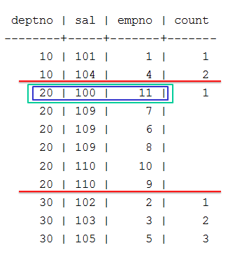
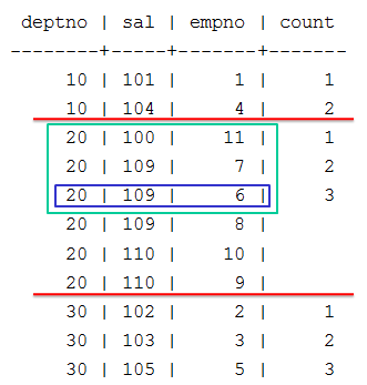
The query returns results that are divided into three partitions, indicated below as red lines. Within the second partition (deptno=20), COUNT processes the window frame clause as follows:

1. Creates the first window (green box). This window comprises a single row, as the current row (blue box) is also the the partition's first row. Thus, the value in the count column shows the number of rows in the current window, which is 1:
   

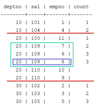
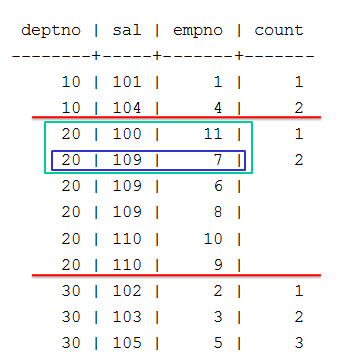
2. After COUNT processes the partition's first row, it resets the current row to the partition's second row. The window now spans the current row and the row above it, so COUNT returns a value of 2:
   

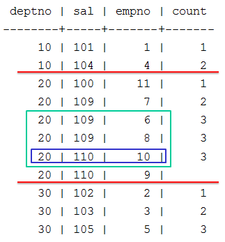
3. After COUNT processes the partition's second row, it resets the current row to the partition's third row. The window now spans the current row and the two rows above it, so COUNT returns a value of 3:
   
   

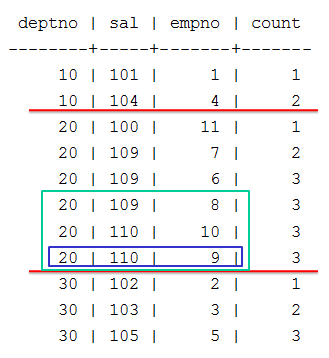
4. Thereafter, COUNT continues to process the remaining partition rows and moves the window accordingly, but the window dimensions (ROWS BETWEEN 2 PRECEDING AND CURRENT ROW) remain unchanged as three rows. Accordingly, the value in the count column also remains unchanged (3):
   
   
   
   
   

2 - Windows with a logical offset (RANGE)

The RANGE keyword defines an analytic window frame as a logical offset from the current row.

For each row, an analytic function uses the window order clause (ORDER_BY) column or expression to calculate window frame dimensions as follows:

1. Within the current partition, evaluates the ORDER_BY value of the current row against the ORDER_BY values of contiguous rows.

2. Determines which of these rows satisfy the specified range requirements relative to the current row.

3. Creates a window frame that includes only those rows.

4. Executes on the current window.

Example

This example uses the table property_sales, which contains data about neighborhood home sales:

=> SELECT property_key, neighborhood, sell_price FROM property_sales ORDER BY neighborhood, sell_price;
 property_key | neighborhood  | sell_price
--------------+---------------+------------
        10918 | Jamaica Plain |     353000
        10921 | Jamaica Plain |     450000
        10927 | Jamaica Plain |     450000
        10922 | Jamaica Plain |     474000
        10919 | Jamaica Plain |     515000
        10917 | Jamaica Plain |     675000
        10924 | Jamaica Plain |     675000
        10920 | Jamaica Plain |     705000
        10923 | Jamaica Plain |     710000
        10926 | Jamaica Plain |     875000
        10925 | Jamaica Plain |     900000
        10930 | Roslindale    |     300000
        10928 | Roslindale    |     422000
        10932 | Roslindale    |     450000
        10929 | Roslindale    |     485000
        10931 | Roslindale    |     519000
        10938 | West Roxbury  |     479000
        10933 | West Roxbury  |     550000
        10937 | West Roxbury  |     550000
        10934 | West Roxbury  |     574000
        10935 | West Roxbury  |     598000
        10936 | West Roxbury  |     615000
        10939 | West Roxbury  |     720000
(23 rows)

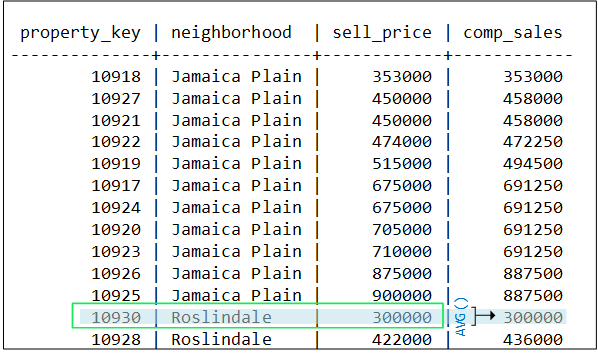
The analytic function AVG can obtain the average of proximate selling prices within each neighborhood. The following query calculates for each home the average sale for all other neighborhood homes whose selling price was $50k higher or lower:

=> SELECT property_key, neighborhood, sell_price, AVG(sell_price) OVER(
     PARTITION BY neighborhood ORDER BY sell_price
     RANGE BETWEEN 50000 PRECEDING and 50000 FOLLOWING)::int AS comp_sales
     FROM property_sales ORDER BY neighborhood;
 property_key | neighborhood  | sell_price | comp_sales
--------------+---------------+------------+------------
        10918 | Jamaica Plain |     353000 |     353000
        10927 | Jamaica Plain |     450000 |     458000
        10921 | Jamaica Plain |     450000 |     458000
        10922 | Jamaica Plain |     474000 |     472250
        10919 | Jamaica Plain |     515000 |     494500
        10917 | Jamaica Plain |     675000 |     691250
        10924 | Jamaica Plain |     675000 |     691250
        10920 | Jamaica Plain |     705000 |     691250
        10923 | Jamaica Plain |     710000 |     691250
        10926 | Jamaica Plain |     875000 |     887500
        10925 | Jamaica Plain |     900000 |     887500
        10930 | Roslindale    |     300000 |     300000
        10928 | Roslindale    |     422000 |     436000
        10932 | Roslindale    |     450000 |     452333
        10929 | Roslindale    |     485000 |     484667
        10931 | Roslindale    |     519000 |     502000
        10938 | West Roxbury  |     479000 |     479000
        10933 | West Roxbury  |     550000 |     568000
        10937 | West Roxbury  |     550000 |     568000
        10934 | West Roxbury  |     574000 |     577400
        10935 | West Roxbury  |     598000 |     577400
        10936 | West Roxbury  |     615000 |     595667
        10939 | West Roxbury  |     720000 |     720000
(23 rows)

AVG processes this query as follows:

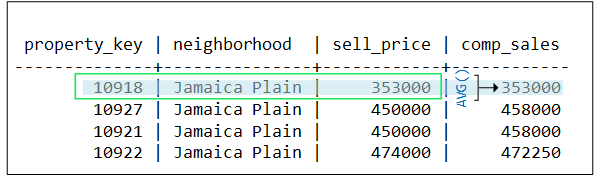
1. AVG evaluates row 1 of the first partition (Jamaica Plain), but finds no sales within $50k of this row's sell_price, ($353k). AVG creates a window that includes this row only, and returns an average of 353k for row 1:
   
   

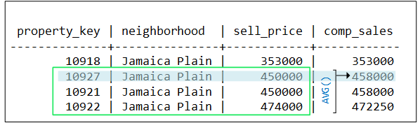
2. AVG evaluates row 2 and finds three sell_price values within $50k of the current row. AVG creates a window that includes these three rows, and returns an average of 458k for row 2:
   

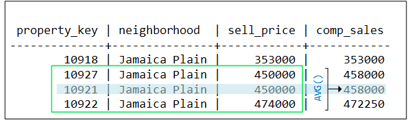
3. AVG evaluates row 3 and finds the same three sell_price values within $50k of the current row. AVG creates a window identical to the one before, and returns the same average of 458k for row 3:
   
   

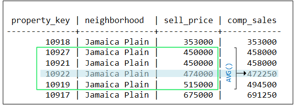
4. AVG evaluates row 4 and finds four sell_price values within $50k of the current row. AVG expands its window to include rows 2 through 5, and returns an average of $472.25k for row 4:
   

5. In similar fashion, AVG evaluates the remaining rows in this partition. When the function evaluates the first row of the second partition (Roslindale), it resets the window as follows:
   
   

Restrictions

If RANGE specifies a constant value, that value's data type and the window's ORDER BY data type must be the same. The following exceptions apply:

• RANGE can specify INTERVAL Year to Month if the window order clause data type is one of following: TIMESTAMP, TIMESTAMP WITH TIMEZONE, or DATE. TIME and TIME WITH TIMEZONE are not supported.

• RANGE can specify INTERVAL Day to Second if the window order clause data is one of following: TIMESTAMP, TIMESTAMP WITH TIMEZONE, DATE, TIME, or TIME WITH TIMEZONE.

The window order clause must specify one of the following data types: NUMERIC, DATE/TIME, FLOAT or INTEGER. This requirement is ignored if the window specifies one of following frames:

• RANGE BETWEEN UNBOUNDED PRECEDING AND CURRENT ROW

• RANGE BETWEEN CURRENT ROW AND UNBOUNDED FOLLOWING

• RANGE BETWEEN UNBOUNDED PRECEDING AND UNBOUNDED FOLLOWING

3 - Reporting aggregates

Some of the analytic functions that take the window-frame-clause are the reporting aggregates. These functions let you compare a partition's aggregate values with detail rows, taking the place of correlated subqueries or joins.

• AVG()

• COUNT()

• MAX() and MIN()

• SUM()

• STDDEV(), STDDEV_POP(), and STDDEV_SAMP()

• VARIANCE(), VAR_POP(), and VAR_SAMP()

If you use a window aggregate with an empty OVER() clause, the analytic function is used as a reporting function, where the entire input is treated as a single partition.

About standard deviation and variance functions

With standard deviation functions, a low standard deviation indicates that the data points tend to be very close to the mean, whereas high standard deviation indicates that the data points are spread out over a large range of values.

Standard deviation is often graphed and a distributed standard deviation creates the classic bell curve.

Variance functions measure how far a set of numbers is spread out.

Examples

Think of the window for reporting aggregates as a window defined as UNBOUNDED PRECEDING and UNBOUNDED FOLLOWING. The omission of a window-order-clause makes all rows in the partition also the window (reporting aggregates).

=> SELECT deptno, sal, empno, COUNT(sal)
  OVER (PARTITION BY deptno) AS COUNT FROM emp;
 deptno | sal | empno | count
--------+-----+-------+-------
     10 | 101 |     1 |     2
     10 | 104 |     4 |     2
------------------------------
     20 | 110 |    10 |     6
     20 | 110 |     9 |     6
     20 | 109 |     7 |     6
     20 | 109 |     6 |     6
     20 | 109 |     8 |     6
     20 | 100 |    11 |     6
------------------------------
     30 | 105 |     5 |     3
     30 | 103 |     3 |     3
     30 | 102 |     2 |     3
(11 rows)

If the OVER() clause in the above query contained a window-order-clause (for example, ORDER BY sal), it would become a moving window (window aggregate) query with a default window of RANGE BETWEEN UNBOUNDED PRECEDING AND CURRENT ROW:

=> SELECT deptno, sal, empno, COUNT(sal)  OVER (PARTITION BY deptno ORDER BY sal) AS COUNT FROM emp;
 deptno | sal | empno | count
--------+-----+-------+-------
     10 | 101 |     1 |     1
     10 | 104 |     4 |     2
------------------------------
     20 | 100 |    11 |     1
     20 | 109 |     7 |     4
     20 | 109 |     6 |     4
     20 | 109 |     8 |     4
     20 | 110 |    10 |     6
     20 | 110 |     9 |     6
------------------------------
     30 | 102 |     2 |     1
     30 | 103 |     3 |     2
     30 | 105 |     5 |     3
(11 rows)

What about LAST_VALUE?

You might wonder why you couldn't just use the LAST_VALUE() analytic function.

For example, for each employee, get the highest salary in the department:

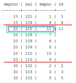
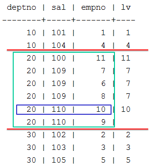
=> SELECT deptno, sal, empno,LAST_VALUE(empno) OVER (PARTITION BY deptno ORDER BY sal) AS lv FROM emp;
![](/images/reporting-aggregates2.png)

Due to default window semantics, LAST_VALUE does not always return the last value of a partition. If you omit the window-frame-clause from the analytic clause, LAST_VALUE operates on this default window. Results, therefore, can seem non-intuitive because the function does not return the bottom of the current partition. It returns the bottom of the window, which continues to change along with the current input row being processed.

Remember the default window:

OVER (PARTITION BY deptno ORDER BY sal)

is the same as:

OVER(PARTITION BY deptno ORDER BY salROWS BETWEEN UNBOUNDED PRECEDING AND CURRENT ROW)

If you want to return the last value of a partition, use UNBOUNDED PRECEDING AND UNBOUNDED FOLLOWING.

=> SELECT deptno, sal, empno, LAST_VALUE(empno)
OVER (PARTITION BY deptno ORDER BY sal
ROWS BETWEEN UNBOUNDED PRECEDING AND UNBOUNDED FOLLOWING) AS lv
FROM emp;
![](/images/reporting-aggregates9.png)

Vertica recommends that you use LAST_VALUE with the window-order-clause to produce deterministic results.

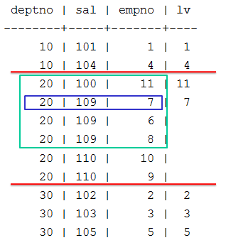
In the following example, empno 6, 7, and 8 have the same salary, so they are in adjacent rows. empno 8 appears first in this case but the order is not guaranteed.

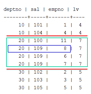
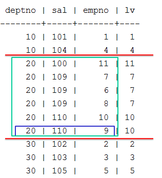
Notice in the output above, the last value is 7, which is the last row from the partition deptno = 20. If the rows have a different order, then the function returns a different value:

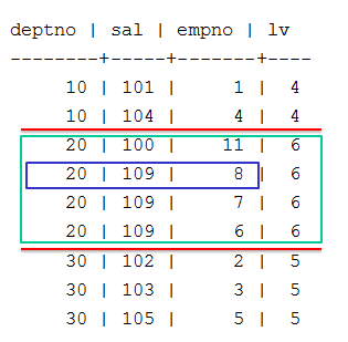
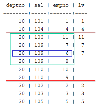
Now the last value is 6, which is the last row from the partition deptno = 20. The solution is to add a unique key to the sort order. Even if the order of the query changes, the result will always be the same, and so deterministic.

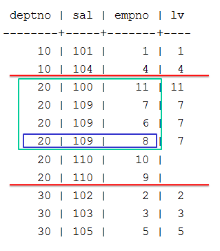
=> SELECT deptno, sal, empno, LAST_VALUE(empno)
OVER (PARTITION BY deptno ORDER BY sal, empno 
ROWS BETWEEN UNBOUNDED PRECEDING AND UNBOUNDED FOLLOWING) as lv
FROM emp;

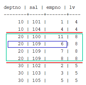
Notice how the rows are now ordered by empno, the last value stays at 8, and it does not matter the order of the query.