Query plans

• 1: Viewing query plans
• 1.1: EXPLAIN-Generated query plans
• 1.2: JSON-Formatted query plans
• 1.3: Verbose query plans
• 1.4: Local query plans
• 2: Query plan cost estimation
• 3: Query plan information and structure
• 3.1: Query plan statistics
• 3.2: Cost and rows path
• 3.3: Projection path
• 3.4: Join path
• 3.5: Path ID
• 3.6: Filter path
• 3.7: GROUP BY paths
• 3.7.1: GROUPBY HASH query plan
• 3.7.2: GROUPBY PIPELINED query plan
• 3.8: Sort path
• 3.9: Limit path
• 3.10: Data redistribution path
• 3.11: Analytic function path
• 3.12: Node down information
• 3.13: MERGE path

1 - Viewing query plans

You can obtain query plans in two ways:

• The EXPLAIN statement outputs query plans in various text formats (see below).
• Management Console provides a graphical interface for viewing query plans. For detailed information, see Working with query plans in MC.

You can also observe the real-time flow of data through a query plan by querying the system table QUERY_PLAN_PROFILES. For more information, see Profiling query plans.

EXPLAIN output options

By default, EXPLAIN output represents the query plan as a hierarchy, where each level, or path, represents a single database operation that the optimizer uses to execute a query. EXPLAIN output also appends DOT language source so you can display this output graphically with open source Graphviz tools.

EXPLAIN supports options for producing verbose and JSON output. You can also show the local query plans that are assigned to each node, which together comprise the total (global) query plan.

EXPLAIN also supports an ANNOTATED option. EXPLAIN ANNOTATED returns a query with embedded optimizer hints, which encapsulate the query plan for this query. For an example of usage, see Using optimizer-generated and custom directed queries together.

1.1 - EXPLAIN-Generated query plans

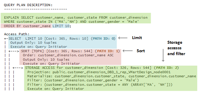
EXPLAIN returns the optimizer's query plan for executing a specified query. For example:

 QUERY PLAN DESCRIPTION:
 ------------------------------

 EXPLAIN SELECT customer_name, customer_state FROM customer_dimension WHERE customer_state IN ('MA','NH') AND customer_gender='Male' ORDER BY customer_name LIMIT 10;

 Access Path:
 +-SELECT  LIMIT 10 [Cost: 365, Rows: 10] (PATH ID: 0)
 |  Output Only: 10 tuples
 |  Execute on: Query Initiator
 | +---> SORT [TOPK] [Cost: 365, Rows: 544] (PATH ID: 1)
 | |      Order: customer_dimension.customer_name ASC
 | |      Output Only: 10 tuples
 | |      Execute on: Query Initiator
 | | +---> STORAGE ACCESS for customer_dimension [Cost: 326, Rows: 544] (PATH ID: 2)
 | | |      Projection: public.customer_dimension_DBD_1_rep_VMartDesign_node0001
 | | |      Materialize: customer_dimension.customer_state, customer_dimension.customer_name
 | | |      Filter: (customer_dimension.customer_gender = 'Male')
 | | |      Filter: (customer_dimension.customer_state = ANY (ARRAY['MA', 'NH']))
 | | |      Execute on: Query Initiator
 | | |      Runtime Filter: (SIP1(TopK): customer_dimension.customer_name)

You can use EXPLAIN to evaluate choices that the optimizer makes with respect to a given query. If you think query performance is less than optimal, run it through the Database Designer. For more information, see Incremental Design and Reducing query run time.

1.2 - JSON-Formatted query plans

EXPLAIN JSON returns a query plan in JSON format. For example:

=> EXPLAIN JSON SELECT customer_name, customer_state FROM customer_dimension
     WHERE customer_state IN ('MA','NH') AND customer_gender='Male' ORDER BY customer_name LIMIT 10;
 ------------------------------
{
     "PARAMETERS" : {
         "QUERY_STRING" : "EXPLAIN JSON SELECT customer_name, customer_state FROM customer_dimension \n
         WHERE customer_state IN ('MA','NH') AND customer_gender='Male' ORDER BY customer_name LIMIT 10;"
     },
     "PLAN" : {
         "PATH_ID" : 0,
         "PATH_NAME" : "SELECT",
         "EXTRA" : " LIMIT 10",
         "COST" : 2114.000000,
         "ROWS" : 10.000000,
         "COST_STATUS" : "NO_STATISTICS",
         "TUPLE_LIMIT" : 10,
         "EXECUTE_NODE" : "Query Initiator",
         "INPUT" : {
             "PATH_ID" : 1,
             "PATH_NAME" : "SORT",
             "EXTRA" : "[TOPK]",
             "COST" : 2114.000000,
             "ROWS" : 49998.000000,
             "COST_STATUS" : "NO_STATISTICS",
             "ORDER" : ["customer_dimension.customer_name", "customer_dimension.customer_state"],
             "TUPLE_LIMIT" : 10,
             "EXECUTE_NODE" : "All Nodes",
             "INPUT" : {
                 "PATH_ID" : 2,
                 "PATH_NAME" : "STORAGE ACCESS",
                 "EXTRA" : "for customer_dimension",
                 "COST" : 252.000000,
                 "ROWS" : 49998.000000,
                 "COST_STATUS" : "NO_STATISTICS",
                 "TABLE" : "public.customer_dimension",
                 "PROJECTION" : "public.customer_dimension_b0",
                 "MATERIALIZE" : ["customer_dimension.customer_name", "customer_dimension.customer_state"],
                 "FILTER" : ["(customer_dimension.customer_state = ANY (ARRAY['MA', 'NH']))", "(customer_dimension.customer_gender = 'Male')"],
                 "EXECUTE_NODE" : "All Nodes"
          "SIP" : "Runtime Filter: (SIP1(TopK): customer_dimension.customer_name)"

             }
         }
     }
 }
(40 rows)

1.3 - Verbose query plans

You can qualify EXPLAIN with the VERBOSE option. This option, valid for default and JSON output, increases the amount of detail in the rendered query plan

For example, the following EXPLAIN statement specifies to produce verbose output. Added information is set off in bold:

=> EXPLAIN VERBOSE SELECT customer_name, customer_state FROM customer_dimension
     WHERE customer_state IN ('MA','NH') AND customer_gender='Male' ORDER BY customer_name LIMIT 10;

QUERY PLAN DESCRIPTION:
 ------------------------------

 Opt Vertica Options
 --------------------
 PLAN_OUTPUT_SUPER_VERBOSE

 EXPLAIN VERBOSE SELECT customer_name, customer_state FROM customer_dimension
 WHERE customer_state IN ('MA','NH') AND customer_gender='Male'
 ORDER BY customer_name LIMIT 10;

Access Path:
+-SELECT  LIMIT 10 [Cost: 756.000000, Rows: 10.000000 Disk(B): 0.000000 CPU(B): 0.000000 Memory(B): 0.000000 Netwrk(B): 0.000000 Parallelism: 1.000000] [OutRowSz (B): 274](PATH ID: 0)
|  Output Only: 10 tuples
|  Execute on: Query Initiator
|  Sort Key: (customer_dimension.customer_name)
|  LDISTRIB_UNSEGMENTED
| +---> SORT [TOPK] [Cost: 756.000000, Rows: 9998.000000 Disk(B): 0.000000 CPU(B): 34274697.123457 Memory(B): 2739452.000000 Netwrk(B): 0.000000 Parallelism: 4.000000 (NO STATISTICS)] [OutRowSz (B): 274] (PATH ID: 1)
| |      Order: customer_dimension.customer_name ASC
| |      Output Only: 10 tuples
| |      Execute on: Query Initiator
| |      Sort Key: (customer_dimension.customer_name)
| |      LDISTRIB_UNSEGMENTED
| | +---> STORAGE ACCESS for customer_dimension [Cost: 513.000000, Rows: 9998.000000 Disk(B): 0.000000 CPU(B): 0.000000 Memory(B): 0.000000 Netwrk(B): 0.000000 Parallelism: 4.000000 (NO STATISTICS)] [OutRowSz (B): 274] (PATH ID: 2)
| | |      Column Cost Aspects: [ Disk(B): 7371817.156569 CPU(B): 4914708.578284 Memory(B): 2659466.004399 Netwrk(B): 0.000000 Parallelism: 4.000000 ]
| | |      Projection: public.customer_dimension_P1
| | |      Materialize: customer_dimension.customer_state, customer_dimension.customer_name
| | |      Filter: (customer_dimension.customer_gender = 'Male')/* sel=0.999800 ndv= 500 */
| | |      Filter: (customer_dimension.customer_state = ANY (ARRAY['MA', 'NH']))/* sel=0.999800 ndv= 500 */
| | |      Execute on: All Nodes
| | |      Runtime Filter: (SIP1(TopK): customer_dimension.customer_name)
| | |      Sort Key: (customer_dimension.household_id, customer_dimension.customer_key, customer_dimension.store_membership_card, customer_dimension.customer_type, customer_dimension.customer_region, customer_dimension.title, customer_dimension.number_of_children)
| | |      LDISTRIB_SEGMENTED

1.4 - Local query plans

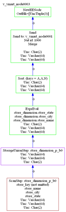
EXPLAIN LOCAL (on a multi-node database) shows the local query plans assigned to each node, which together comprise the total (global) query plan. If you omit this option, Vertica shows only the global query plan. Local query plans are shown only in DOT language source, which can be rendered in Graphviz.

For example, the following EXPLAIN statement includes the LOCAL option:

=> EXPLAIN LOCAL SELECT store_name, store_city, store_state
   FROM store.store_dimension ORDER BY store_state ASC, store_city ASC;

The output includes GraphViz source, which describes the local query plans assigned to each node. For example, output for this statement on a three-node database includes a GraphViz description of the following query plan for one node (v_vmart_node0003):

 -----------------------------------------------
 PLAN: v_vmart_node0003 (GraphViz Format)
 -----------------------------------------------
 digraph G {
 graph [rankdir=BT, label = "v_vmart_node0003\n", labelloc=t, labeljust=l ordering=out]
 0[label = "NewEENode \nOutBlk=[UncTuple(3)]", color = "green", shape = "box"];
 1[label = "Send\nSend to: v_vmart_node0001\nNet id: 1000\nMerge\n\nUnc: Char(2)\nUnc: Varchar(64)\nUnc: Varchar(64)", color = "green", shape = "box"];
 2[label = "Sort: (keys = A,A,N)\nUnc: Char(2)\nUnc: Varchar(64)\nUnc: Varchar(64)", color = "green", shape = "box"];
 3[label = "ExprEval: \n  store_dimension.store_state\n  store_dimension.store_city\n  store_dimension.store_name\nUnc: Char(2)\nUnc: Varchar(64)\nUnc: Varchar(64)
", color = "green", shape = "box"];
 4[label = "StorageUnionStep: store_dimension_p_b0\nUnc: Varchar(64)\nUnc: Varchar(64)\nUnc: Char(2)", color = "purple", shape = "box"];
 5[label = "ScanStep: store_dimension_p_b0\nstore_key (not emitted)\nstore_name\nstore_city\nstore_state\nUnc: Varchar(64)\nUnc: Varchar(64)\nUnc: Char(2)", color
= "brown", shape = "box"];
 1->0 [label = "0",color = "blue"];
 2->1 [label = "0",color = "blue"];
 3->2 [label = "0",color = "blue"];
 4->3 [label = "0",color = "blue"];
 5->4 [label = "0",color = "blue"];
 }

GraphViz renders this output as follows:

2 - Query plan cost estimation

The query optimizer chooses a query plan based on cost estimates. The query optimizer uses information from a number of sources to develop potential plans and determine their relative costs. These include:

• Number of table rows

• Column statistics, including: number of distinct values (cardinality), minimum/maximum values, distribution of values, and disk space usage

• Access path that is likely to require fewest I/O operations, and lowest CPU, memory, and network usage

• Available eligible projections

• Join options: join types (merge versus hash joins), join order

• Query predicates

• Data segmentation across cluster nodes

Many important optimizer decisions rely on statistics, which the query optimizer uses to determine the final plan to execute a query. Therefore, it is important that statistics be up to date. Without reasonably accurate statistics, the optimizer could choose a suboptimal plan, which might affect query performance.

Vertica provides hints about statistics in the query plan. See Query plan statistics.

Cost versus execution runtime

Although costs correlate to query runtime, they do not provide an estimate of actual runtime. For example, if the optimizer determines that Plan A costs twice as much as Plan B, it is likely that Plan A will require more time to run. However, this cost estimate does not necessarily indicate that Plan A will run twice as long as Plan B.

Also, plan costs for different queries are not directly comparable. For example, if the estimated cost of Plan X for query1 is greater than the cost of Plan Y for query2, it is not necessarily true that Plan X's runtime is greater than Plan Y's runtime.

3 - Query plan information and structure

Depending on the query and database schema, EXPLAIN output includes the following information:

• Tables referenced by the statement

• Estimated costs

• Estimated row cardinality

• Path ID, an integer that links to error messages and profiling counters so you troubleshoot performance issues more easily. For more information, see Profiling query plans.

• Data operations such as SORT, FILTER, LIMIT, and GROUP BY

• Projections used

• Information about statistics—for example, whether they are current or out of range

• Algorithms chosen for operations into the query, such as HASH/MERGE or GROUPBY HASH/GROUPBY PIPELINED

• Data redistribution (broadcast, segmentation) across cluster nodes

Example

In the EXPLAIN output that follows, the optimizer processes a query in three steps, where each step identified by a unique path ID:

• 0: Limit

• 1: Sort

• 2: Storage access and filter

3.1 - Query plan statistics

If you query a table whose statistics are unavailable or out-of-date, the optimizer might choose a sub-optimal query plan.

You can resolve many issues related to table statistics by calling ANALYZE_STATISTICS. This function let you update statistics at various scopes: one or more table columns, a single table, or all database tables.

If you update statistics and find that the query still performs sub-optimally, run your query through Database Designer and choose incremental design as the design type.

For detailed information about updating database statistics, see Collecting database statistics.

Statistics hints in query plans

Query plans can contain information about table statistics through two hints: NO STATISTICS and STALE STATISTICS. For example, the following query plan fragment includes NO STATISTICS to indicate that histograms are unavailable:

| | +-- Outer -> STORAGE ACCESS for fact [Cost: 604, Rows: 10K (NO STATISTICS)]

The following query plan fragment includes STALE STATISTICS to indicate that the predicate has fallen outside the histogram range:

| | +-- Outer -> STORAGE ACCESS for fact [Cost: 35, Rows: 1 (STALE STATISTICS)]

3.2 - Cost and rows path

The following EXPLAIN output shows the Cost operator:

 Access Path: +-SELECT  LIMIT 10 [Cost: 370, Rows: 10] (PATH ID: 0)
 |  Output Only: 10 tuples
 |  Execute on: Query Initiator
 | +---> SORT [Cost: 370, Rows: 544] (PATH ID: 1)
 | |      Order: customer_dimension.customer_name ASC
 | |      Output Only: 10 tuples
 | |      Execute on: Query Initiator
 | | +---> STORAGE ACCESS for customer_dimension [Cost: 331, Rows: 544] (PATH ID: 2)
 | | |      Projection: public.customer_dimension_DBD_1_rep_vmartdb_design_vmartdb_design_node0001
 | | |      Materialize: customer_dimension.customer_state, customer_dimension.customer_name
 | | |      Filter: (customer_dimension.customer_gender = 'Male')
 | | |      Filter: (customer_dimension.customer_state = ANY (ARRAY['MA', 'NH']))
 | | |      Execute on: Query Initiator

The Row operator is the number of rows the optimizer estimates the query will return. Letters after numbers refer to the units of measure (K=thousand, M=million, B=billion, T=trillion), so the output for the following query indicates that the number of rows to return is 50 thousand.

=> EXPLAIN SELECT customer_gender FROM customer_dimension;
 Access Path:
 +-STORAGE ACCESS for customer_dimension [Cost: 17, Rows: 50K (3 RLE)] (PATH ID: 1)
 |  Projection: public.customer_dimension_DBD_1_rep_vmartdb_design_vmartdb_design_node0001
 |  Materialize: customer_dimension.customer_gender
 |  Execute on: Query Initiator

The reference to (3 RLE) in the STORAGE ACCESS path means that the optimizer estimates that the storage access operator returns 50K rows. Because the column is run-length encoded (RLE), the real number of RLE rows returned is only three rows:

• 1 row for female

• 1 row for male

• 1 row that represents unknown (NULL) gender

3.3 - Projection path

You can see which projections the optimizer chose for the query plan by looking at the Projection path in the textual output:

EXPLAIN SELECT
   customer_name,
   customer_state
 FROM customer_dimension
 WHERE customer_state in ('MA','NH')
 AND customer_gender = 'Male'
 ORDER BY customer_name
 LIMIT 10;
 Access Path:
 +-SELECT  LIMIT 10 [Cost: 370, Rows: 10] (PATH ID: 0)
 |  Output Only: 10 tuples
 |  Execute on: Query Initiator
 | +---> SORT [Cost: 370, Rows: 544] (PATH ID: 1)
 | |      Order: customer_dimension.customer_name ASC
 | |      Output Only: 10 tuples
 | |      Execute on: Query Initiator
 | | +---> STORAGE ACCESS for customer_dimension [Cost: 331, Rows: 544] (PATH ID: 2)
 | | |      Projection: public.customer_dimension_DBD_1_rep_vmart_vmart_node0001
 | | |      Materialize: customer_dimension.customer_state, customer_dimension.customer_name
 | | |      Filter: (customer_dimension.customer_gender = 'Male')
 | | |      Filter: (customer_dimension.customer_state = ANY (ARRAY['MA', 'NH']))
 | | |      Execute on: Query Initiator

The query optimizer automatically picks the best projections, but without reasonably accurate statistics, the optimizer could choose a suboptimal projection or join order for a query. For details, see Collecting Statistics.

Vertica considers which projection to choose for a plan by considering the following aspects:

• How columns are joined in the query

• How the projections are grouped or sorted

• Whether SQL analytic operations applied

• Any column information from a projection's storage on disk

As Vertica scans the possibilities for each plan, projections with the higher initial costs could end up in the final plan because they make joins cheaper. For example, a query can be answered with many possible plans, which the optimizer considers before choosing one of them. For efficiency, the optimizer uses sophisticated algorithms to prune intermediate partial plan fragments with higher cost. The optimizer knows that intermediate plan fragments might initially look bad (due to high storage access cost) but which produce excellent final plans due to other optimizations that it allows.

If your statistics are up to date but the query still performs poorly, run the query through the Database Designer. For details, see Incremental Design.

Tips

• To test different segmented projections, refer to the projection by name in the query.

• For optimal performance, write queries so the columns are sorted the same way that the projection columns are sorted.

See also

• Reducing query run time
• Creating custom designs
• Projections

3.4 - Join path

Just like a join query, which references two or more tables, the Join step in a query plan has two input branches:

• The left input, which is the outer table of the join

• The right input, which is the inner table of the join

In the following query, the T1 table is the left input because it is on the left side of the JOIN keyword, and the T2 table is the right input, because it is on the right side of the JOIN keyword:

SELECT * FROM T1 JOIN T2 ON T1.x = T2.x;

Outer versus inner join

Query performance is better if the small table is used as the inner input to the join. The query optimizer automatically reorders the inputs to joins to ensure that this is the case unless the join in question is an outer join.

The following example shows a query and its plan for a left outer join:

=> EXPLAIN SELECT CD.annual_income,OSI.sale_date_key
-> FROM online_sales.online_sales_fact OSI
-> LEFT OUTER JOIN customer_dimension CD ON CD.customer_key = OSI.customer_key;
 Access Path:
 +-JOIN HASH [LeftOuter] [Cost: 4K, Rows: 5M] (PATH ID: 1)
 |  Join Cond: (CD.customer_key = OSI.customer_key)
 |  Materialize at Output: OSI.sale_date_key
 |  Execute on: All Nodes
 | +-- Outer -> STORAGE ACCESS for OSI [Cost: 3K, Rows: 5M] (PATH ID: 2)
 | |      Projection: online_sales.online_sales_fact_DBD_12_seg_vmartdb_design_vmartdb_design
 | |      Materialize: OSI.customer_key
 | |      Execute on: All Nodes
 | +-- Inner -> STORAGE ACCESS for CD [Cost: 264, Rows: 50K] (PATH ID: 3)
 | |      Projection: public.customer_dimension_DBD_1_rep_vmartdb_design_vmartdb_design_node0001
 | |      Materialize: CD.annual_income, CD.customer_key
 | |      Execute on: All Nodes

The following example shows a query and its plan for a full outer join:

=> EXPLAIN SELECT CD.annual_income,OSI.sale_date_key
-> FROM online_sales.online_sales_fact OSI
-> FULL OUTER JOIN customer_dimension CD ON CD.customer_key = OSI.customer_key;
 Access Path:
 +-JOIN HASH [FullOuter] [Cost: 18K, Rows: 5M] (PATH ID: 1) Outer (RESEGMENT) Inner (FILTER)
 |  Join Cond: (CD.customer_key = OSI.customer_key)
 |  Execute on: All Nodes
 | +-- Outer -> STORAGE ACCESS for OSI [Cost: 3K, Rows: 5M] (PATH ID: 2)
 | |      Projection: online_sales.online_sales_fact_DBD_12_seg_vmartdb_design_vmartdb_design
 | |      Materialize: OSI.sale_date_key, OSI.customer_key
 | |      Execute on: All Nodes
 | +-- Inner -> STORAGE ACCESS for CD [Cost: 264, Rows: 50K] (PATH ID: 3)
 | |      Projection: public.customer_dimension_DBD_1_rep_vmartdb_design_vmartdb_design_node0001
 | |      Materialize: CD.annual_income, CD.customer_key
 | |      Execute on: All Nodes

Hash and merge joins

Vertica has two join algorithms to choose from: merge join and hash join. The optimizer automatically chooses the most appropriate algorithm, given the query and projections in a system.

For the following query, the optimizer chooses a hash join.

=> EXPLAIN SELECT CD.annual_income,OSI.sale_date_key
-> FROM online_sales.online_sales_fact OSI
-> INNER JOIN customer_dimension CD ON CD.customer_key = OSI.customer_key;
 Access Path:
 +-JOIN HASH [Cost: 4K, Rows: 5M] (PATH ID: 1)
 |  Join Cond: (CD.customer_key = OSI.customer_key)
 |  Materialize at Output: OSI.sale_date_key
 |  Execute on: All Nodes
 | +-- Outer -> STORAGE ACCESS for OSI [Cost: 3K, Rows: 5M] (PATH ID: 2)
 | |      Projection: online_sales.online_sales_fact_DBD_12_seg_vmartdb_design_vmartdb_design
 | |      Materialize: OSI.customer_key
 | |      Execute on: All Nodes
 | +-- Inner -> STORAGE ACCESS for CD [Cost: 264, Rows: 50K] (PATH ID: 3)
 | |      Projection: public.customer_dimension_DBD_1_rep_vmartdb_design_vmartdb_design_node0001
 | |      Materialize: CD.annual_income, CD.customer_key
 | |      Execute on: All Nodes

In the next example, the optimizer chooses a merge join. The optimizer's first pass performs a merge join because the inputs are presorted, and then it performs a hash join.

=> EXPLAIN SELECT count(*) FROM online_sales.online_sales_fact OSI
-> INNER JOIN customer_dimension CD ON CD.customer_key = OSI.customer_key
-> INNER JOIN product_dimension PD ON PD.product_key = OSI.product_key;
 Access Path:
 +-GROUPBY NOTHING [Cost: 8K, Rows: 1] (PATH ID: 1)
 |  Aggregates: count(*)
 |  Execute on: All Nodes
 | +---> JOIN HASH [Cost: 7K, Rows: 5M] (PATH ID: 2)
 | |      Join Cond: (PD.product_key = OSI.product_key)
 | |      Materialize at Input: OSI.product_key
 | |      Execute on: All Nodes
 | | +-- Outer -> JOIN MERGEJOIN(inputs presorted) [Cost: 4K, Rows: 5M] (PATH ID: 3)
 | | |      Join Cond: (CD.customer_key = OSI.customer_key)
 | | |      Execute on: All Nodes
 | | | +-- Outer -> STORAGE ACCESS for OSI [Cost: 3K, Rows: 5M] (PATH ID: 4)
 | | | |      Projection: online_sales.online_sales_fact_DBD_12_seg_vmartdb_design_vmartdb_design
 | | | |      Materialize: OSI.customer_key
 | | | |      Execute on: All Nodes
 | | | +-- Inner -> STORAGE ACCESS for CD [Cost: 132, Rows: 50K] (PATH ID: 5)
 | | | |      Projection: public.customer_dimension_DBD_1_rep_vmartdb_design_vmartdb_design_node0001
 | | | |      Materialize: CD.customer_key
 | | | |      Execute on: All Nodes
 | | +-- Inner -> STORAGE ACCESS for PD [Cost: 152, Rows: 60K] (PATH ID: 6)
 | | |      Projection: public.product_dimension_DBD_2_rep_vmartdb_design_vmartdb_design_node0001
 | | |      Materialize: PD.product_key
 | | |      Execute on: All Nodes

Inequality joins

Vertica processes joins with equality predicates very efficiently. The query plan shows equality join predicates as join condition (Join Cond).

=> EXPLAIN SELECT CD.annual_income, OSI.sale_date_key
-> FROM online_sales.online_sales_fact OSI
-> INNER JOIN customer_dimension CD
-> ON CD.customer_key = OSI.customer_key;
 Access Path:
 +-JOIN HASH [Cost: 4K, Rows: 5M] (PATH ID: 1)
 |  Join Cond: (CD.customer_key = OSI.customer_key)
 |  Materialize at Output: OSI.sale_date_key
 |  Execute on: All Nodes
 | +-- Outer -> STORAGE ACCESS for OSI [Cost: 3K, Rows: 5M] (PATH ID: 2)
 | |      Projection: online_sales.online_sales_fact_DBD_12_seg_vmartdb_design_vmartdb_design
 | |      Materialize: OSI.customer_key
 | |      Execute on: All Nodes
 | +-- Inner -> STORAGE ACCESS for CD [Cost: 264, Rows: 50K] (PATH ID: 3)
 | |      Projection: public.customer_dimension_DBD_1_rep_vmartdb_design_vmartdb_design_node0001
 | |      Materialize: CD.annual_income, CD.customer_key
 | |      Execute on: All Nodes

However, inequality joins are treated like cross joins and can run less efficiently, which you can see by the change in cost between the two queries:

=> EXPLAIN SELECT CD.annual_income, OSI.sale_date_key
-> FROM online_sales.online_sales_fact OSI
-> INNER JOIN customer_dimension CD
-> ON CD.customer_key < OSI.customer_key;
 Access Path:
 +-JOIN HASH [Cost: 98M, Rows: 5M] (PATH ID: 1)
 |  Join Filter: (CD.customer_key < OSI.customer_key)
 |  Materialize at Output: CD.annual_income
 |  Execute on: All Nodes
 | +-- Outer -> STORAGE ACCESS for CD [Cost: 132, Rows: 50K] (PATH ID: 2)
 | |      Projection: public.customer_dimension_DBD_1_rep_vmartdb_design_vmartdb_design_node0001
 | |      Materialize: CD.customer_key
 | |      Execute on: All Nodes
 | +-- Inner -> STORAGE ACCESS for OSI [Cost: 3K, Rows: 5M] (PATH ID: 3)
 | |      Projection: online_sales.online_sales_fact_DBD_12_seg_vmartdb_design_vmartdb_design
 | |      Materialize: OSI.sale_date_key, OSI.customer_key
 | |      Execute on: All Nodes

Event series joins

Event series joins are denoted by the INTERPOLATED path.

=> EXPLAIN SELECT * FROM hTicks h FULL OUTER JOIN aTicks a -> ON (h.time INTERPOLATE PREVIOUS
 Access Path:
 +-JOIN  (INTERPOLATED) [FullOuter] [Cost: 31, Rows: 4 (NO STATISTICS)] (PATH ID: 1)
   Outer (SORT ON JOIN KEY) Inner (SORT ON JOIN KEY)
 |  Join Cond: (h."time" = a."time")
 |  Execute on: Query Initiator
 | +-- Outer -> STORAGE ACCESS for h [Cost: 15, Rows: 4 (NO STATISTICS)] (PATH ID: 2)
 | |      Projection: public.hTicks_node0004
 | |      Materialize: h.stock, h."time", h.price
 | |      Execute on: Query Initiator
 | +-- Inner -> STORAGE ACCESS for a [Cost: 15, Rows: 4 (NO STATISTICS)] (PATH ID: 3)
 | |      Projection: public.aTicks_node0004
 | |      Materialize: a.stock, a."time", a.price
 | |      Execute on: Query Initiator

3.5 - Path ID

The PATH ID is a unique identifier that Vertica assigns to each operation (path) within a query plan. The same identifier is shared by:

• Query plans

• Join error messages

• System tables EXECUTION_ENGINE_PROFILES and QUERY_PLAN_PROFILES

Path IDs can help you trace issues to their root cause. For example, if a query returns a join error, preface the query with EXPLAIN and look for PATH ID n in the query plan to see which join in the query had the problem.

For example, the following EXPLAIN output shows the path ID for each path in the optimizer's query plan:

=> EXPLAIN SELECT * FROM fact JOIN dim ON x=y JOIN ext on y=z;
 Access Path:
 +-JOIN MERGEJOIN(inputs presorted) [Cost: 815, Rows: 10K (NO STATISTICS)] (PATH ID: 1)
 | Join Cond: (dim.y = ext.z)
 | Materialize at Output: fact.x
 | Execute on: All Nodes
 | +-- Outer -> JOIN MERGEJOIN(inputs presorted) [Cost: 408, Rows: 10K (NO STATISTICS)] (PATH ID: 2)
 | | Join Cond: (fact.x = dim.y)
 | | Execute on: All Nodes
 | | +-- Outer -> STORAGE ACCESS for fact [Cost: 202, Rows: 10K (NO STATISTICS)] (PATH ID: 3)
 | | | Projection: public.fact_super
 | | | Materialize: fact.x
 | | | Execute on: All Nodes
 | | +-- Inner -> STORAGE ACCESS for dim [Cost: 202, Rows: 10K (NO STATISTICS)] (PATH ID: 4)
 | | | Projection: public.dim_super
 | | | Materialize: dim.y
 | | | Execute on: All Nodes
 | +-- Inner -> STORAGE ACCESS for ext [Cost: 202, Rows: 10K (NO STATISTICS)] (PATH ID: 5)
 | | Projection: public.ext_super
 | | Materialize: ext.z
 | | Execute on: All Nodes

3.6 - Filter path

The Filter step evaluates predicates on a single table. It accepts a set of rows, eliminates some of them (based on the criteria you provide in your query), and returns the rest. For example, the optimizer can filter local data of a join input that will be joined with another re-segmented join input.

The following statement queries the customer_dimension table and uses the WHERE clause to filter the results only for male customers in Massachusetts and New Hampshire.

EXPLAIN SELECT
  CD.customer_name,
  CD.customer_state,
  AVG(CD.customer_age) AS avg_age,
  COUNT(*) AS count
FROM customer_dimension CD
WHERE CD.customer_state in ('MA','NH') AND CD.customer_gender = 'Male'
GROUP BY CD.customer_state, CD.customer_name;

The query plan output is as follows:

 Access Path:
 +-GROUPBY HASH [Cost: 378, Rows: 544] (PATH ID: 1)
 |  Aggregates: sum_float(CD.customer_age), count(CD.customer_age), count(*)
 |  Group By: CD.customer_state, CD.customer_name
 |  Execute on: Query Initiator
 | +---> STORAGE ACCESS for CD [Cost: 372, Rows: 544] (PATH ID: 2)
 | |      Projection: public.customer_dimension_DBD_1_rep_vmartdb_design_vmartdb_design_node0001
 | |      Materialize: CD.customer_state, CD.customer_name, CD.customer_age
 | |      Filter: (CD.customer_gender = 'Male')
 | |      Filter: (CD.customer_state = ANY (ARRAY['MA', 'NH']))
 | |      Execute on: Query Initiator

3.7 - GROUP BY paths

A GROUP BY operation has two algorithms:

• GROUPBY HASH input is not sorted by the group columns, so Vertica builds a hash table on those group columns in order to process the aggregates and group by expressions.

• GROUPBY PIPELINED requires that inputs be presorted on the columns specified in the group, which means that Vertica need only retain data in the current group in memory. GROUPBY PIPELINED operations are preferred because they are generally faster and require less memory than GROUPBY HASH. GROUPBY PIPELINED is especially useful for queries that process large numbers of high-cardinality group by columns or DISTINCT aggregates.

If possible, the query optimizer chooses the faster algorithm GROUPBY PIPELINED over GROUPBY HASH.

3.7.1 - GROUPBY HASH query plan

Here's an example of how GROUPBY HASH operations look in EXPLAIN output.

=> EXPLAIN SELECT COUNT(DISTINCT annual_income)
     FROM customer_dimension
     WHERE customer_region='NorthWest';

The output shows that the optimizer chose the less efficient GROUPBY HASH path, which means the projection was not presorted on the annual_income column. If such a projection is available, the optimizer would choose the GROUPBY PIPELINED algorithm.

Access Path:
+-GROUPBY NOTHING [Cost: 256, Rows: 1 (NO STATISTICS)] (PATH ID: 1)
|  Aggregates: count(DISTINCT customer_dimension.annual_income)
| +---> GROUPBY HASH (LOCAL RESEGMENT GROUPS) [Cost: 253, Rows: 10K (NO STATISTICS)] (PATH ID: 2)
| |      Group By: customer_dimension.annual_income
| | +---> STORAGE ACCESS for customer_dimension [Cost: 227, Rows: 50K (NO STATISTICS)] (PATH ID: 3)
| | |      Projection: public.customer_dimension_super
| | |      Materialize: customer_dimension.annual_income
| | |      Filter: (customer_dimension.customer_region = 'NorthWest'
...

3.7.2 - GROUPBY PIPELINED query plan

If you have a projection that is already sorted on the customer_gender column, the optimizer chooses the faster GROUPBY PIPELINED operation:

 => EXPLAIN SELECT COUNT(distinct customer_gender) from customer_dimension;
Access Path:
 +-GROUPBY NOTHING [Cost: 22, Rows: 1] (PATH ID: 1)
 |  Aggregates: count(DISTINCT customer_dimension.customer_gender)
 |  Execute on: Query Initiator
 | +---> GROUPBY PIPELINED [Cost: 20, Rows: 10K] (PATH ID: 2)
 | |      Group By: customer_dimension.customer_gender
 | |      Execute on: Query Initiator
 | | +---> STORAGE ACCESS for customer_dimension [Cost: 17, Rows: 50K (3 RLE)] (PATH ID: 3)
 | | |      Projection: public.customer_dimension_DBD_1_rep_vmartdb_design_vmartdb_design_node0001
 | | |      Materialize: customer_dimension.customer_gender
 | | |      Execute on: Query Initiator

Similarly, the use of an equality predicate, such as in the following query, preserves GROUPBY PIPELINED:

=> EXPLAIN SELECT COUNT(DISTINCT annual_income)    FROM customer_dimension
   WHERE customer_gender = 'Female';

 Access Path: +-GROUPBY NOTHING [Cost: 161, Rows: 1] (PATH ID: 1)
 |  Aggregates: count(DISTINCT customer_dimension.annual_income)
 | +---> GROUPBY PIPELINED [Cost: 158, Rows: 10K] (PATH ID: 2)
 | |      Group By: customer_dimension.annual_income
 | | +---> STORAGE ACCESS for customer_dimension [Cost: 144, Rows: 47K] (PATH ID: 3)
 | | |      Projection: public.customer_dimension_DBD_1_rep_vmartdb_design_vmartdb_design_node0001
 | | |      Materialize: customer_dimension.annual_income
 | | |      Filter: (customer_dimension.customer_gender = 'Female')

3.8 - Sort path

The SORT operator sorts the data according to a specified list of columns. The EXPLAIN output indicates the sort expressions and if the sort order is ascending (ASC) or descending (DESC).

For example, the following query plan shows the column list nature of the SORT operator:

EXPLAIN SELECT
  CD.customer_name,
  CD.customer_state,
  AVG(CD.customer_age) AS avg_age,
  COUNT(*) AS count
FROM customer_dimension CD
WHERE CD.customer_state in ('MA','NH')
  AND CD.customer_gender = 'Male'
GROUP BY CD.customer_state, CD.customer_name
ORDER BY avg_age, customer_name;
 Access Path:
 +-SORT [Cost: 422, Rows: 544] (PATH ID: 1)
 |  Order: (<SVAR> / float8(<SVAR>)) ASC, CD.customer_name ASC
 |  Execute on: Query Initiator
 | +---> GROUPBY HASH [Cost: 378, Rows: 544] (PATH ID: 2)
 | |      Aggregates: sum_float(CD.customer_age), count(CD.customer_age), count(*)
 | |      Group By: CD.customer_state, CD.customer_name
 | |      Execute on: Query Initiator
 | | +---> STORAGE ACCESS for CD [Cost: 372, Rows: 544] (PATH ID: 3)
 | | |      Projection: public.customer_dimension_DBD_1_rep_vmart_vmart_node0001
 | | |      Materialize: CD.customer_state, CD.customer_name, CD.customer_age
 | | |      Filter: (CD.customer_gender = 'Male')
 | | |      Filter: (CD.customer_state = ANY (ARRAY['MA', 'NH']))
 | | |      Execute on: Query Initiator

If you change the sort order to descending, the change appears in the query plan:

EXPLAIN SELECT
  CD.customer_name,
  CD.customer_state,
  AVG(CD.customer_age) AS avg_age,
  COUNT(*) AS count
FROM customer_dimension CD
WHERE CD.customer_state in ('MA','NH')
  AND CD.customer_gender = 'Male'
GROUP BY CD.customer_state, CD.customer_name
ORDER BY avg_age DESC, customer_name;
 Access Path:
 +-SORT [Cost: 422, Rows: 544] (PATH ID: 1)
 |  Order: (<SVAR> / float8(<SVAR>)) DESC, CD.customer_name ASC
 |  Execute on: Query Initiator
 | +---> GROUPBY HASH [Cost: 378, Rows: 544] (PATH ID: 2)
 | |      Aggregates: sum_float(CD.customer_age), count(CD.customer_age), count(*)
 | |      Group By: CD.customer_state, CD.customer_name
 | |      Execute on: Query Initiator
 | | +---> STORAGE ACCESS for CD [Cost: 372, Rows: 544] (PATH ID: 3)
 | | |      Projection: public.customer_dimension_DBD_1_rep_vmart_vmart_node0001
 | | |      Materialize: CD.customer_state, CD.customer_name, CD.customer_age
 | | |      Filter: (CD.customer_gender = 'Male')
 | | |      Filter: (CD.customer_state = ANY (ARRAY['MA', 'NH']))
 | | |      Execute on: Query Initiator

3.9 - Limit path

The LIMIT path restricts the number of result rows based on the LIMIT clause in the query. Using the LIMIT clause in queries with thousands of rows might increase query performance.

The optimizer pushes the LIMIT operation as far down as possible in queries. A single LIMIT clause in the query can generate multiple Output Only plan annotations.

 => EXPLAIN SELECT COUNT(DISTINCT annual_income) FROM customer_dimension LIMIT 10;
Access Path:
 +-SELECT  LIMIT 10 [Cost: 161, Rows: 10] (PATH ID: 0)
 |  Output Only: 10 tuples
 | +---> GROUPBY NOTHING [Cost: 161, Rows: 1] (PATH ID: 1)
 | |      Aggregates: count(DISTINCT customer_dimension.annual_income)
 | |      Output Only: 10 tuples
 | | +---> GROUPBY HASH (SORT OUTPUT) [Cost: 158, Rows: 10K] (PATH ID: 2)
 | | |      Group By: customer_dimension.annual_income
 | | | +---> STORAGE ACCESS for customer_dimension [Cost: 132, Rows: 50K] (PATH ID: 3)
 | | | |      Projection: public.customer_dimension_DBD_1_rep_vmartdb_design_vmartdb_design_node0001
 | | | |      Materialize: customer_dimension.annual_income

3.10 - Data redistribution path

The optimizer can redistribute join data in two ways:

• Broadcasting

• Resegmentation

Broadcasting

Broadcasting sends a complete copy of an intermediate result to all nodes in the cluster. Broadcast is used for joins in the following cases:

• One table is very small (usually the inner table) compared to the other.

• Vertica can avoid other large upstream resegmentation operations.

• Outer join or subquery semantics require one side of the join to be replicated.

For example:

=> EXPLAIN SELECT * FROM T1 LEFT JOIN T2 ON T1.a > T2.y;
 Access Path:
 +-JOIN HASH [LeftOuter] [Cost: 40K, Rows: 10K (NO STATISTICS)] (PATH ID: 1) Inner (BROADCAST)
 |  Join Filter: (T1.a > T2.y)
 |  Materialize at Output: T1.b
 |  Execute on: All Nodes
 | +-- Outer -> STORAGE ACCESS for T1 [Cost: 151, Rows: 10K (NO STATISTICS)] (PATH ID: 2)
 | |      Projection: public.T1_b0
 | |      Materialize: T1.a
 | |      Execute on: All Nodes
 | +-- Inner -> STORAGE ACCESS for T2 [Cost: 302, Rows: 10K (NO STATISTICS)] (PATH ID: 3)
 | |      Projection: public.T2_b0
 | |      Materialize: T2.x, T2.y
 | |      Execute on: All Nodes

Resegmentation

Resegmentation takes an existing projection or intermediate relation and resegments the data evenly across all cluster nodes. At the end of the resegmentation operation, every row from the input relation is on exactly one node. Resegmentation is the operation used most often for distributed joins in Vertica if the data is not already segmented for local joins. For more detail, see Identical segmentation.

For example:

=> CREATE TABLE T1 (a INT, b INT) SEGMENTED BY HASH(a) ALL NODES;
=> CREATE TABLE T2 (x INT, y INT) SEGMENTED BY HASH(x) ALL NODES;
=> EXPLAIN SELECT * FROM T1 JOIN T2 ON T1.a = T2.y;

 ------------------------------ QUERY PLAN DESCRIPTION: ------------------------------
 Access Path:
 +-JOIN HASH [Cost: 639, Rows: 10K (NO STATISTICS)] (PATH ID: 1) Inner (RESEGMENT)
 |  Join Cond: (T1.a = T2.y)
 |  Materialize at Output: T1.b
 |  Execute on: All Nodes
 | +-- Outer -> STORAGE ACCESS for T1 [Cost: 151, Rows: 10K (NO STATISTICS)] (PATH ID: 2)
 | |      Projection: public.T1_b0
 | |      Materialize: T1.a
 | |      Execute on: All Nodes
 | +-- Inner -> STORAGE ACCESS for T2 [Cost: 302, Rows: 10K (NO STATISTICS)] (PATH ID: 3)
 | |      Projection: public.T2_b0
 | |      Materialize: T2.x, T2.y
 | |      Execute on: All Nodes

3.11 - Analytic function path

Vertica attempts to optimize multiple SQL-99 Analytic functions from the same query by grouping them together in Analytic Group areas.

For each analytical group, Vertica performs a distributed sort and resegment of the data, if necessary.

You can tell how many sorts and resegments are required based on the query plan.

For example, the following query plan shows that the FIRST_VALUE and LAST_VALUE functions are in the same analytic group because their OVER clause is the same. In contrast, ROW_NUMBER() has a different ORDER BY clause, so it is in a different analytic group. Because both groups share the same PARTITION BY deal_stage clause, the data does not need to be resegmented between groups :

EXPLAIN SELECT
  first_value(deal_size) OVER (PARTITION BY deal_stage
  ORDER BY deal_size),
  last_value(deal_size) OVER (PARTITION BY deal_stage
  ORDER BY deal_size),
  row_number() OVER (PARTITION BY deal_stage
  ORDER BY largest_bill_amount)
  FROM customer_dimension;

 Access Path:
 +-ANALYTICAL [Cost: 1K, Rows: 50K] (PATH ID: 1)
 |  Analytic Group
 |   Functions: row_number()
 |   Group Sort: customer_dimension.deal_stage ASC, customer_dimension.largest_bill_amount ASC NULLS LAST
 |  Analytic Group
 |   Functions: first_value(), last_value()
 |   Group Filter: customer_dimension.deal_stage
 |   Group Sort: customer_dimension.deal_stage ASC, customer_dimension.deal_size ASC NULL LAST
 |  Execute on: All Nodes
 | +---> STORAGE ACCESS for customer_dimension [Cost: 263, Rows: 50K]
         (PATH ID: 2)
 | |      Projection: public.customer_dimension_DBD_1_rep_vmart_vmart_node0001
 | |      Materialize: customer_dimension.largest_bill_amount,
          customer_dimension.deal_stage, customer_dimension.deal_size
 | |      Execute on: All Nodes

See also

3.12 - Node down information

Vertica provides performance optimization when cluster nodes fail by distributing the work of the down nodes uniformly among available nodes throughout the cluster.

When a node in your cluster is down, the query plan identifies which node the query will execute on. To help you quickly identify down nodes on large clusters, EXPLAIN output lists up to six nodes, if the number of running nodes is less than or equal to six, and lists only down nodes if the number of running nodes is more than six.

The following table provides more detail:

Examples

In the following example, the down node is v_vmart_node0005, and the node v_vmart_node0006 will execute this run of the query.

=> EXPLAIN SELECT * FROM test;
QUERY PLAN
-----------------------------------------------------------------------------
QUERY PLAN DESCRIPTION:
------------------------------
EXPLAIN SELECT * FROM my1table;
Access Path:
+-STORAGE ACCESS for my1table [Cost: 10, Rows: 2] (PATH ID: 1)
| Projection: public.my1table_b0
| Materialize: my1table.c1, my1table.c2
| Execute on: All Except v_vmart_node0005
+-STORAGE ACCESS for my1table (REPLACEMENT FOR DOWN NODE) [Cost: 66, Rows: 2]
| Projection: public.my1table_b1
| Materialize: my1table.c1, my1table.c2
| Execute on: v_vmart_node0006

The All Permanent Nodes output in the following example fragment denotes that the node list is for permanent (non-ephemeral) nodes only:

=> EXPLAIN SELECT * FROM my2table;
Access Path:
+-STORAGE ACCESS for my2table [Cost: 18, Rows:6 (NO STATISTICS)] (PATH ID: 1)
|  Projection: public.my2tablee_b0
|  Materialize: my2table.x, my2table.y, my2table.z
|  Execute on: All Permanent Nodes

3.13 - MERGE path

Vertica prepares an optimized query plan for a MERGE statement if the statement and its tables meet the criteria described in MERGE optimization.

Use the EXPLAIN keyword to determine whether Vertica can produce an optimized query plan for a given MERGE statement. If optimization is possible, the EXPLAIN-generated output contains a[Semi] path, as shown in the following sample fragment:

...
Access Path:
+-DML DELETE [Cost: 0, Rows: 0]
|  Target Projection: public.A_b1 (DELETE ON CONTAINER)
|  Target Prep:
|  Execute on: All Nodes
| +---> JOIN MERGEJOIN(inputs presorted) [Semi] [Cost: 6, Rows: 1 (NO STATISTICS)] (PATH ID: 1)
         Inner (RESEGMENT)
| |      Join Cond: (A.a1 = VAL(2))
| |      Execute on: All Nodes
| | +-- Outer -> STORAGE ACCESS for A [Cost: 2, Rows: 2 (NO STATISTICS)] (PATH ID: 2)
...

Conversely, if Vertica cannot create an optimized plan, EXPLAIN-generated output contains RightOuter path:

...
Access Path: +-DML MERGE
 |  Target Projection: public.locations_b1
 |  Target Projection: public.locations_b0
 |  Target Prep:
 |  Execute on: All Nodes
 | +---> JOIN MERGEJOIN(inputs presorted) [RightOuter] [Cost: 28, Rows: 3 (NO STATISTICS)] (PATH ID: 1) Outer (RESEGMENT) Inner (RESEGMENT)
 | |      Join Cond: (locations.user_id = VAL(2)) AND (locations.location_x = VAL(2)) AND (locations.location_y = VAL(2))
 | |      Execute on: All Nodes
 | | +-- Outer -> STORAGE ACCESS for <No Alias> [Cost: 15, Rows: 2 (NO STATISTICS)] (PATH ID: 2)
...