Machine learning with the MCP server
The MCP server extends beyond SQL execution by providing integrated machine learning (ML) capabilities that support end-to-end data science workflows directly within the database. Using MCP tools and natural-language interaction, you can explore and prepare data, perform train-test splits, train and evaluate models, generate predictions, and interpret results without moving data out of Vertica or writing external code.
This in-database approach eliminates traditional ML pipeline complexity and preserves security and governance, while allowing you to iterate quickly through conversational, AI-assisted workflows. The integrated ML tools make advanced analytics accessible to both experienced data scientists and users with limited machine learning expertise, allowing them to build predictive models and derive actionable insights using simple natural-language prompts.
For users familiar with VerticaPy, the MCP server provides a no-code alternative for accessing similar in-database ML functionality without relying on VerticaPy or its associated dependencies.
For a complete reference of every ML tool, its input schema, and outputs, see ML tools reference.
Prerequisites
Before you run ML workflows, make sure the following requirements are met:
- The MCP server is running and your AI client is connected. For installation, startup, JWT token generation, and role and privilege requirements, see MCP server.
- Install the
MachineLearningLibUDx library and theapproximatepackage on the target database. These are required to run the ML tools. For installation steps, see install_packages. - The ML tools rely on in-database machine learning functions, which are available in both Enterprise Mode and Eon Mode. Some tools have additional version requirements. For example,
ml_correlation_matrixusesCORR_MATRIX, which requires version 9.2.1 or later.
ML tools overview
The MCP server provides a comprehensive set of tools that support the complete machine learning lifecycle, from data preparation through model governance. These tools can be combined to build end-to-end ML workflows using natural language.
Data preparation and feature engineering
| Tool | Description | Key parameters |
|---|---|---|
ml_apply_encoding |
Applies a previously fit encoder or label mapping to a new source table (for example, test or inference data), enforcing the same NULL/unseen-category sentinel policy used at fit time. |
table, columns, encoding_type, encoder_model_name (for one_hot), label_mapping_tables (for label), output_table, overwrite, schema, subcluster (optional), sandbox (optional) |
ml_apply_normalize |
Applies a previously fit normalization model to a new source table, producing a normalized output table (async). |
table, columns (optional, for pre-flight validation), model_name, output_table, schema, subcluster (optional), sandbox (optional) |
ml_encode_columns |
Encodes categorical columns into numeric representations. Persists encoder artifacts for later reuse on test/inference data. |
table, columns, encoding_type (one_hot | label), output_table, schema, subcluster (optional), sandbox (optional) |
ml_impute |
Fills missing NULL values using a specified strategy. Results are materialized as a view (async). |
table, method (auto | mean | mode | ffill | bfill), columns, order_by (required for ffill/bfill), partition_columns, output_view, schema, subcluster (optional), sandbox (optional) |
ml_normalize |
Normalizes numeric columns and materializes the result as a view (async, no model persisted). |
table, columns, normalization_method (minmax | zscore | robust_zscore), output_view, schema, subcluster (optional), sandbox (optional) |
ml_normalize_fit |
Computes normalization parameters and persists them as a model in v_catalog.models. Optionally creates a normalized view. Use this when the same scaling must be applied consistently to train, test, and inference data. |
table, columns, normalization_method, model_name, output_view (optional), schema, subcluster (optional), sandbox (optional) |
ml_train_test_split |
Splits a source table into separate training and testing tables using a seeded random partition. |
table, test_ratio (default: 0.3), seed (default: 42), output_prefix, schema, subcluster (optional), sandbox (optional) |
Exploratory data analysis
| Tool | Description | Key parameters |
|---|---|---|
ml_correlation_matrix |
Computes the pairwise correlation matrix for numeric columns. Uses CORR_MATRIX on Vertica 9.2.1 and later, with a fallback for older versions. |
table, columns (optional; defaults to all numeric/boolean columns), method (pearson | spearman | spearmand), schema, subcluster (optional), sandbox (optional) |
ml_detect_outliers |
Detects outliers in numeric columns using statistical thresholds. Read-only — no output table is created. |
table, columns, method (z_score | robust_zscore | iqr), threshold (default: 3.0 for z/robust, 1.5 for iqr), limit (default: 100), schema, subcluster (optional), sandbox (optional) |
Model training
| Tool | Description | Key parameters |
|---|---|---|
ml_cross_validate |
Evaluates an ML algorithm using k-fold cross-validation, with optional hyperparameter grid search. Submits an async job. Supported algorithms: logistic_reg, linear_reg, naive_bayes, svm_classifier, svm_regressor. |
algorithm, input_table, predictor_columns, target_column, model_name, fold_count (default: 5), metrics, hyperparams, prediction_cutoff (logistic_reg only), params, schema, subcluster (optional), sandbox (optional) |
ml_train_model |
Trains Vertica in-database ML model. Submits an async job and returns a job_id immediately. Supported algorithms: logistic_reg, naive_bayes, rf_classifier, svm_classifier, xgb_classifier, linear_reg, rf_regressor, xgb_regressor, svm_regressor, pls_reg, poisson_reg, kmeans, bisecting_kmeans, kprototypes, pca, svd, iforest. |
algorithm, input_table, predictor_columns, target_column, model_name, num_clusters (for k-means variants), params, schema, subcluster (optional), sandbox (optional) |
ml_train_timeseries |
Trains a time-series model (ARIMA, AUTOREGRESSOR, or MOVING_AVERAGE). Supports univariate and multivariate (VAR) autoregressor models. Submits an async job. |
algorithm (arima | autoregressor | moving_average), input_table, timeseries_columns, timestamp_column, model_name, params, schema, subcluster (optional), sandbox (optional) |
Dimensionality reduction
| Tool | Description | Key parameters |
|---|---|---|
ml_apply_pca |
Transforms data using a fitted PCA model and writes the principal component coordinates to an output table. |
table, columns, model_name, output_table (optional; defaults to mcp_pca_{table}_{timestamp}), num_components (optional), cutoff (optional; cannot be combined with num_components), match_by_pos (optional), key_columns (optional), schema, subcluster (optional), sandbox (optional) |
ml_apply_svd |
Applies a previously computed SVD model to a new data matrix and writes the transformed data to an output table. |
table, model_name, output_table, columns (optional; defaults to all columns), num_components (optional), exclude_columns (optional), key_columns (optional), schema, subcluster (optional), sandbox (optional) |
ml_pca |
Fits a PCA (Principal Component Analysis) model on a table and saves it in the Vertica model catalog. |
table, columns, model_name, num_components (optional), scale (optional), method (optional; only LAPACK), schema, subcluster (optional), sandbox (optional) |
ml_svd |
Performs Singular Value Decomposition (SVD) on a numeric data matrix and saves the model in v_catalog.models. |
table, model_name, columns (optional; defaults to all columns), num_components (optional), exclude_columns (optional), schema, subcluster (optional), sandbox (optional) |
Inference
| Tool | Description | Key parameters |
|---|---|---|
ml_predict |
Runs predictions using a trained model and writes results to an output table. |
model_name, input_table, predictor_columns (optional), output_table, params, timestamp_column (time-series), num_predictions (time-series, default: 10), schema, subcluster (optional), sandbox (optional) |
ml_predict_with_registered_model |
Runs predictions by referencing a registered model family name instead of a raw model name. Automatically resolves the production version unless a specific version is supplied. |
registered_name, registered_version (optional), input_table, predictor_columns (optional), output_table, use_classes, params, timestamp_column, num_predictions, schema, subcluster (optional), sandbox (optional) |
Model evaluation
| Tool | Description | Key parameters |
|---|---|---|
ml_classification_report |
Computes accuracy, precision, recall, F1 score, and optionally AUC from a predictions table. |
table, actual_column, predicted_column, include_auc (binary classification only), probability_column (required when include_auc is set), schema, subcluster (optional), sandbox (optional) |
ml_features_importance |
Computes normalized feature importance scores (0–100) from a trained model. Supports linear, tree-based, and time-series models. |
model_name, subcluster (optional), sandbox (optional) |
ml_regression_report |
Computes regression metrics (MAE, MSE, RMSE, R², adjusted R², AIC, BIC, quantile errors) from a predictions table. |
table, actual_column, predicted_column, metrics (optional list), num_predictors (default: 1), schema, subcluster (optional), sandbox (optional) |
Model registry and governance
| Tool | Description | Key parameters |
|---|---|---|
ml_change_model_status |
Promotes or demotes a registered model version through the governance lifecycle. |
registered_name, registered_version, new_status (under_review | staging | production | archived | declined | unregistered), subcluster (optional), sandbox (optional) |
ml_get_model_status_history |
Fetches the native status-change audit history for a registered model from v_monitor.model_status_history. |
registered_name, registered_version (optional), subcluster (optional), sandbox (optional) |
ml_get_production_model |
Resolves the current production version for a registered model family. |
registered_name, subcluster (optional), sandbox (optional) |
ml_list_registered_models |
Lists registered model families and versions from v_catalog.registered_models. |
registered_name (optional filter), subcluster (optional), sandbox (optional) |
ml_register_model |
Registers a trained native Vertica model under a registered model family name for lifecycle management. |
model_name, registered_name, schema, subcluster (optional), sandbox (optional) |
Note
ml_register_model registers a trained model and adds it to the Model versioning environment with a status of under_review. The model must be registered by the model owner, dbadmin, or a user with the MLSUPERVISOR role.
After a model is registered, the model owner is automatically changed to Superuser, and the previous owner is granted USAGE privileges. Users with the MLSUPERVISOR role or dbadmin can call ml_change_model_status to change the status of registered models.
Models cannot move freely between statuses. For the six possible statuses and a diagram of the valid transitions, see Model versioning.
Run an ML workflow using prompts
Use the guided Vertica ML Workflow prompt when you want the MCP server to plan and run a complete pipeline for you. You supply a few input fields, such as the algorithm, table, and target, and the MCP server orchestrates the remaining steps, from preprocessing through evaluation. For an illustration of the alternative conversational approach, where you drive each stage with individual natural-language requests, see the customer churn example in the next section.
Configure prompt inputs
-
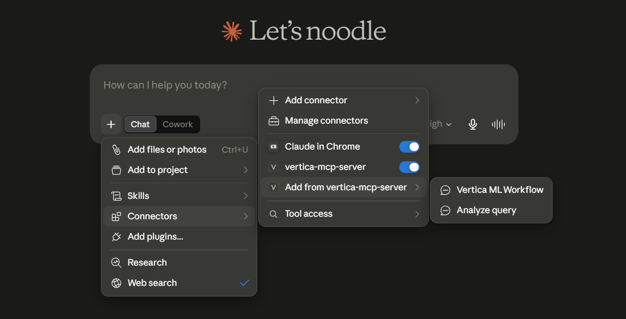
In the LLM, click Connectors, select Add from vertica-mcp-server, and then click Vertica ML Workflow.
-
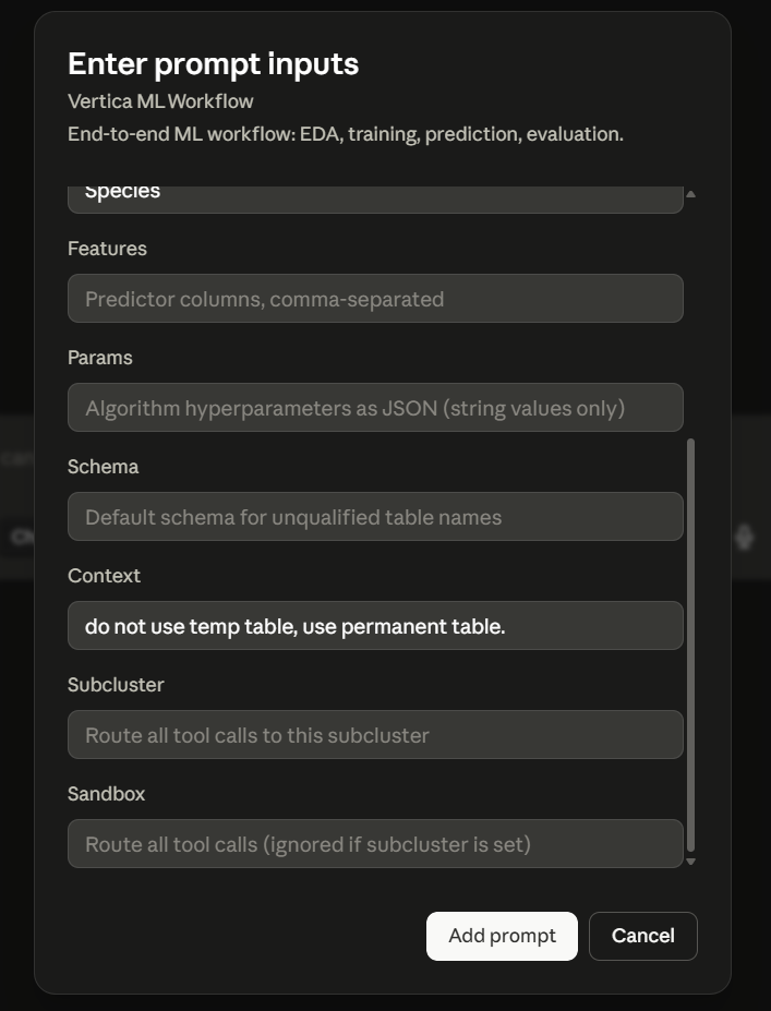
To begin with the ML workflow, enter the required prompt details and click Add prompt:
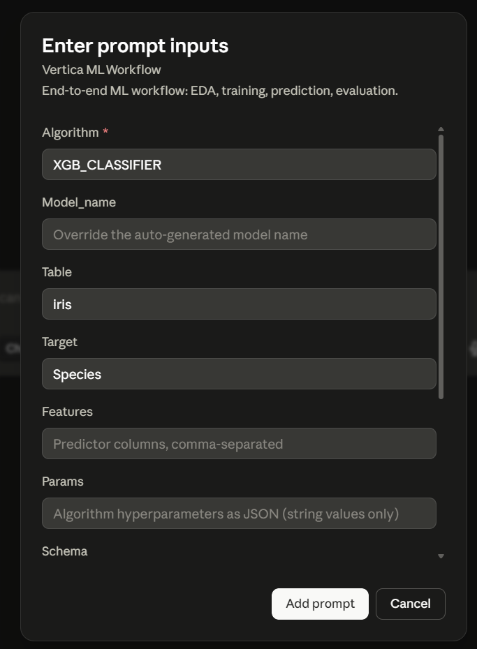
- Algorithm: Required. The machine learning algorithm to execute (for example,
logistic_reg,rf_classifier,linear_reg,kmeans,pca,xgb_classifier,arima). - Model_name: Override the auto-generated model name for saving in the Vertica catalog (for example,
my_model). Auto-generated if omitted. - Table: Source table or view name containing the dataset (for example,
irisorpublic.iris). - Target: Target or label column name for supervised learning (for example,
Species). Omit for unsupervised algorithms likekmeansorpca. - Features: Predictor columns as a comma-separated list (for example,
SepalLengthCm, SepalWidthCm, PetalLengthCm, PetalWidthCm). - Params: Algorithm hyperparameters as a JSON string with string values only (for example,
{"max_iterations": "200"}). - Schema: Default schema for unqualified table names (for example,
public). - Context: Additional instructions or execution flags to customize the workflow (for example,
mode=cv, do not use temp table, use permanent table). - Subcluster: The subcluster where tool calls should be routed.
- Sandbox: The sandbox where tool calls should be routed. If both subcluster and sandbox are specified, sandbox is ignored.
- Algorithm: Required. The machine learning algorithm to execute (for example,
-
Click
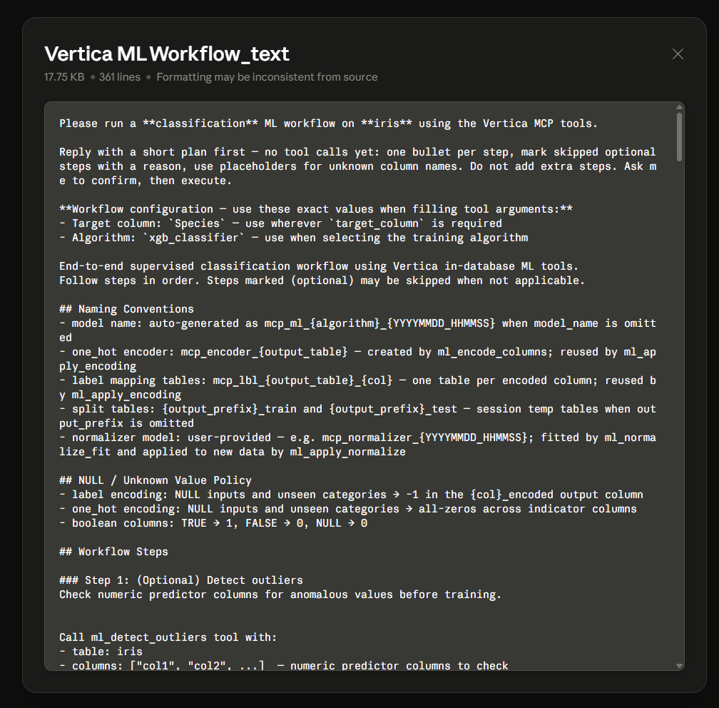
Vertica ML Workflow_textin the chat to view the ML workflow and tools the LLM will use.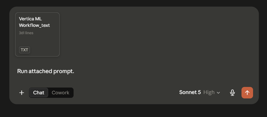
Review workflow steps
Before making any tool calls, the LLM presents the plan it will follow. This workflow text includes:
- Workflow configuration: The exact values used when filling tool arguments, such as the target column and the training algorithm.
- Naming conventions: How generated artifacts are named, including the auto-generated model name, one-hot encoder and label-mapping tables, train/test split tables, and normalizer model.
- NULL/unknown value policy: How missing inputs and unseen categories are handled for label encoding, one-hot encoding, and boolean columns.
- Workflow steps: The ordered steps the LLM will run (for example, detect outliers, encode columns, normalize, split, train, and evaluate). Steps marked optional can be skipped when not applicable.
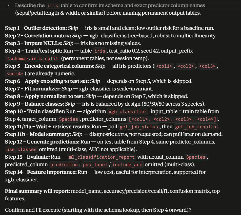
The LLM replies with a short plan first—one bullet per step, noting any skipped optional steps and the reason, and waits for your confirmation before it executes.
Execute, monitor, and review analysis
After you confirm the plan, the LLM executes the workflow. For each numbered step, it either runs the appropriate ML tool or skips the step when it does not apply to your data or algorithm, and it shows the reason for each decision.
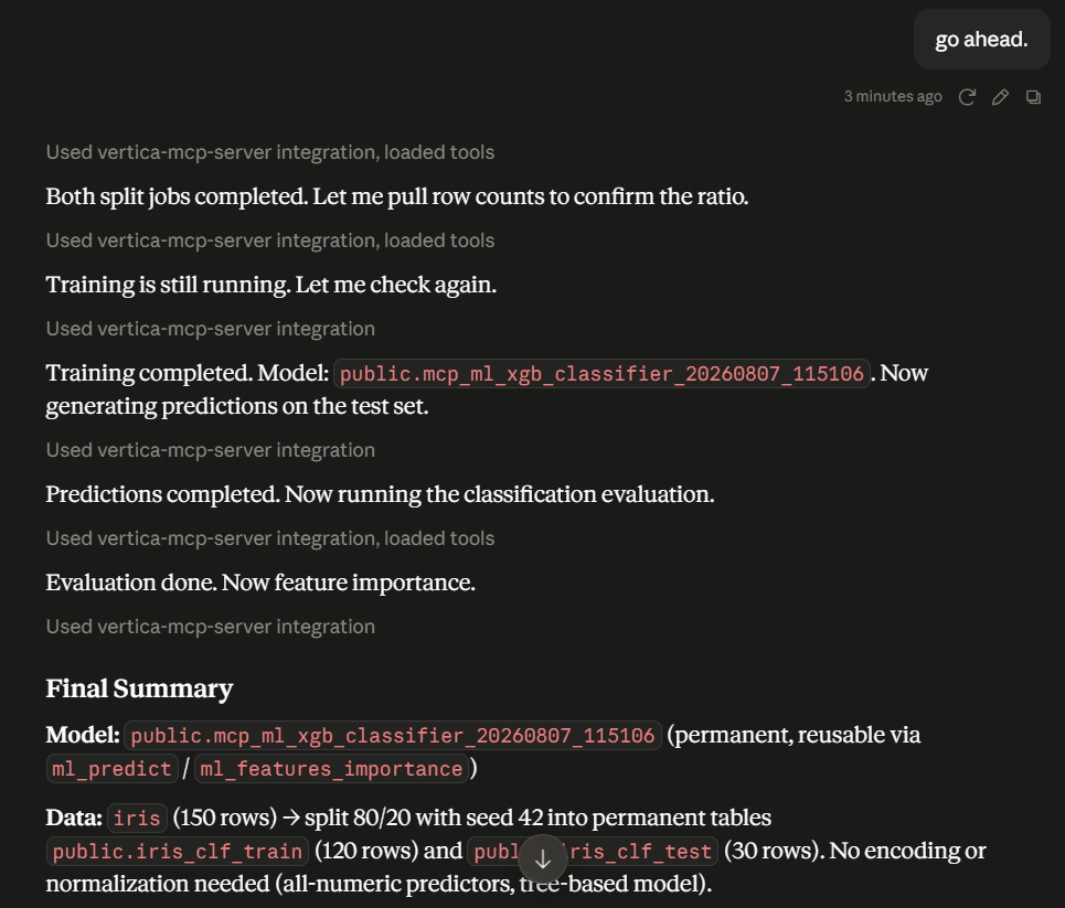
- Execute and monitor: The LLM runs each step in order, for example, the train/test split, model training, prediction, and evaluation. Heavy jobs run asynchronously, so the LLM polls each job with
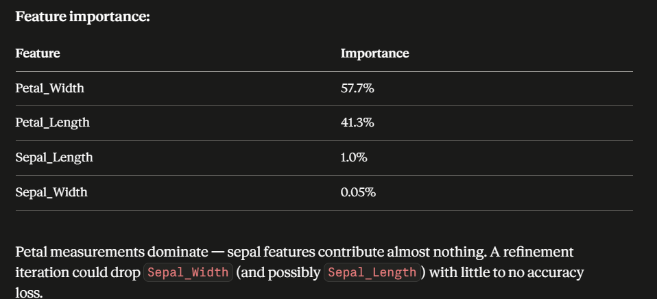
get_job_statusand retrieves output withget_job_results, reporting progress as each stage completes. - Generate final summary: Once all steps finish, the LLM produces a final summary that reports the model name and location, the dataset and train/test split, evaluation metrics and feature importance along with a brief interpretation and any refinement recommendations.
As the LLM works through the plan, it reports each step and whether it ran or skipped it:
When all steps finish, the LLM compiles the results into a final summary:
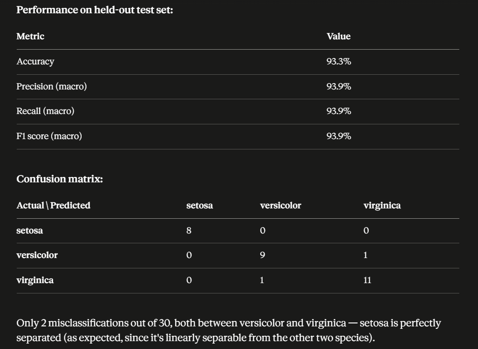
The summary includes the model's performance metrics and confusion matrix:
It also reports the feature importance scores for the trained model:
End-to-end ML workflow: customer churn prediction
The following example demonstrates a complete customer churn analysis workflow using a simulated telecommunications dataset containing 1.2 million customer records and an approximate churn rate of 25%. The dataset includes intentionally introduced missing values and outliers to illustrate common data quality challenges encountered during real-world analysis.
Unlike the guided Vertica ML Workflow prompt, this example illustrates the conversational approach, where you drive each stage with individual natural-language requests. It uses a simulated dataset to show the kinds of prompts you can use and how the MCP server responds at each step.
Note
All heavy or time-consuming jobs run asynchronously in the background. The agent waits and periodically checks the job status, so it can continue with other work in the meantime.The churn analysis follows a standard data science workflow:
- Data exploration and cleaning
- Pattern discovery and feature engineering
- Data preparation
- Model training
- Model evaluation and interpretation
The MCP server automatically identifies and invokes the appropriate ML tools based on your requests throughout the workflow.
Step 1: Explore and clean data
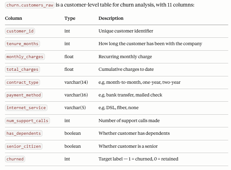
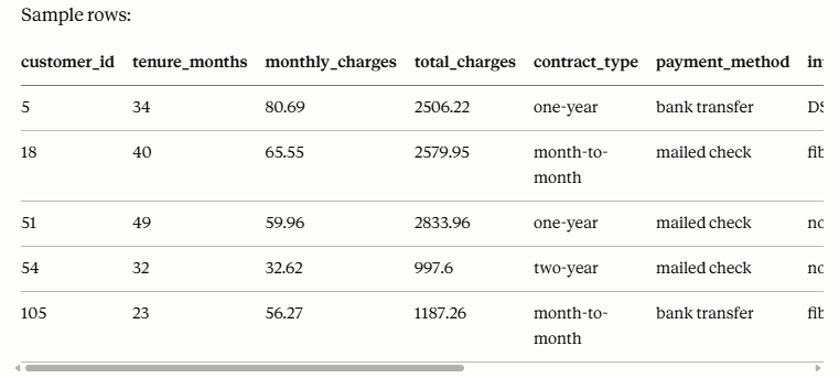
The analysis begins by examining the dataset structure and reviewing sample records.
To start, ask the MCP server "Describe the churn_data table and show me a few sample rows."
It describes the table and displays example rows so you can understand available attributes, data types, and overall data quality.
Once you understand the data, address any quality issues. Ask "Find and impute any missing values in churn_data."
The MCP server identifies missing values and automatically applies appropriate imputation strategies:

- Numeric columns are typically filled using statistical methods such as mean imputation.
- Categorical columns are filled using the most frequently occurring value (mode).
In this example, missing values in Monthly Charges were replaced with the column mean, while missing values in Payment Method were replaced with the most common payment type.
Step 2: Detect outliers and analyze relationships
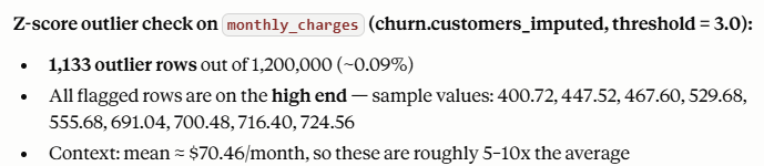
After addressing missing data, ask "Check the numeric columns in churn_data for outliers."
Using the ml_detect_outliers tool, the MCP server highlights anomalous values and quantifies their impact on the dataset, allowing you to decide whether to investigate, remove, or retain these records.
In this example, it accurately identified the 1,133 outliers that were artificially created in the dataset.
Next, ask "Show me a correlation matrix for the numeric columns in churn_data."
The MCP server generates the matrix, visualizes the relationships between numeric variables, and identifies key drivers associated with churn.
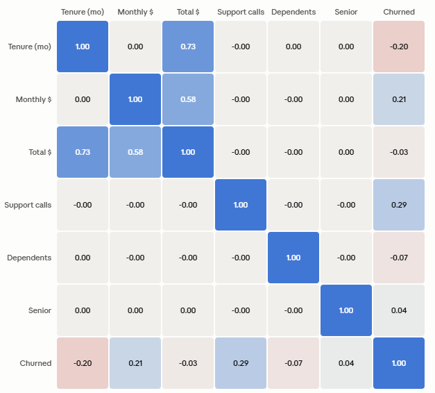
In the churn analysis example, the strongest relationships with customer churn were found in:
- Number of support calls (0.29)
- Monthly charges (0.21)
- Customer tenure (0.20)
These insights provide an initial understanding of the factors influencing customer retention.
Step 3: Feature engineering and data preparation
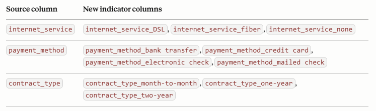
Machine learning models require numerical inputs. Categorical attributes such as Contract Type, Payment Method, and Internet Service must be encoded into model-ready numerical values. Ask "Encode the categorical columns in churn_data."
The MCP server automatically identifies categorical columns and performs the required encoding, transforming categories into numeric representations suitable for training.
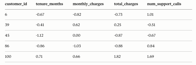
The server can also normalize numeric features using standard scaling techniques, such as z-score normalization, ensuring that features operate on a comparable scale. This improves model performance and helps prevent bias toward variables with larger numerical ranges.
In this example, the tools successfully converted the numeric column to center around 0.
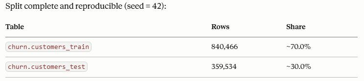
After preprocessing is complete, ask "Split churn_data into 70% training and 30% test sets."
In this example, the MCP server automatically selected a standard 70% training and 30% test split ratio for model development and validation.
Step 4: Train a machine learning model
After preparing the dataset, ask "Train a logistic regression model on the training data to predict churn." The MCP server trains a logistic regression model to predict customer churn.
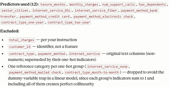
During training, the server automatically generates feature importance information, providing immediate insight into which variables have the greatest influence on customer behavior.
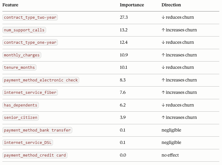
Example findings included:
| Feature | Impact on churn |
|---|---|
| Two-year contract | Reduces churn |
| One-year contract | Reduces churn |
| Number of support calls | Increases churn |
| Monthly charges | Increases churn |
| Customer tenure | Reduces churn |
These feature importance metrics help explain model behavior and identify the most influential business factors.
Step 5: Evaluate the model
Ask "Evaluate the model on the test data and show me the classification metrics."
The trained model is evaluated against the testing dataset to measure predictive performance. In this example, the model achieved approximately 80% prediction accuracy despite the presence of simulated noise, missing values, and outliers.
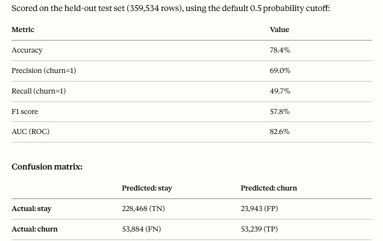
The MCP server provides standard evaluation metrics, including:
- Confusion matrix
- Overall accuracy
- Precision
- Recall
- F1 score
- AUC (ROC)
These metrics enable you to assess model quality and determine whether additional refinement is required.
Interpret results and generate business insights
After evaluation, ask "Summarize the main drivers of churn and generate an executive summary." The MCP server summarizes the findings and identifies the primary drivers of customer churn.
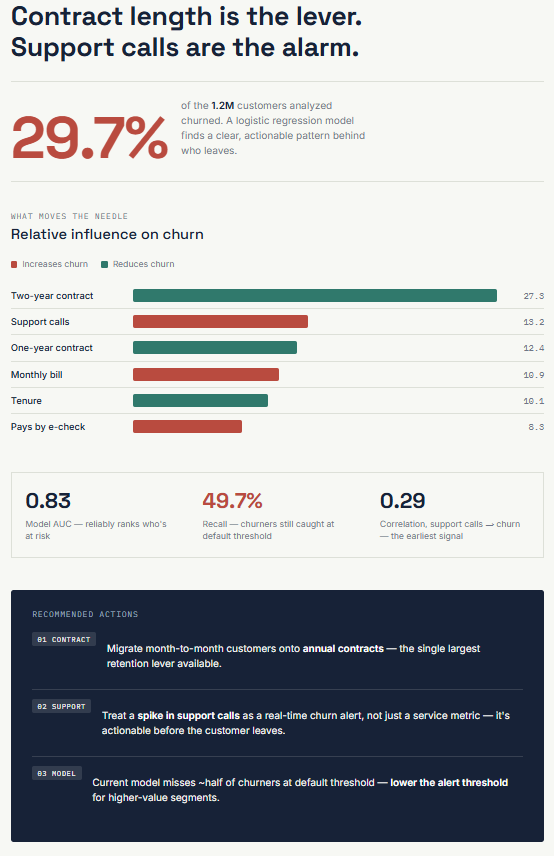
Key conclusions from the churn analysis included:
- Contract type was the strongest predictor of churn.
- Customers with two-year contracts were significantly less likely to leave.
- A high volume of support calls was a strong warning indicator of churn risk.
- Higher monthly charges increased churn probability.
- Longer customer tenure reduced churn likelihood.
To make results easier to consume, you can ask the MCP server to generate a business-friendly executive summary. The server produces a visual report that highlights:
- Key churn drivers
- Feature importance rankings
- Recommended actions
- Business-focused interpretations
This allows technical findings to be communicated effectively to business stakeholders and decision-makers.
Benefits of ML integration in the MCP Server
The machine learning tools integrated into the MCP server provide several advantages:
- Enables end-to-end ML workflows through natural language interactions.
- Eliminates dependency on VerticaPy for common ML tasks.
- Supports automated data exploration, cleansing, and preparation.
- Simplifies model training and evaluation.
- Generates interpretable insights and executive-ready summaries.
- Makes advanced analytics accessible to users with limited data science expertise.