Machine learning for predictive analytics

• 1: Download the machine learning example data
• 2: Data preparation
• 2.1: Balancing imbalanced data
• 2.2: Detect outliers
• 2.3: Encoding categorical columns
• 2.4: Imputing missing values
• 2.5: Normalizing data
• 2.6: PCA (principal component analysis)
• 2.6.1: Dimension reduction using PCA
• 2.7: Sampling data
• 2.8: SVD (singular value decomposition)
• 2.8.1: Computing SVD
• 3: Regression algorithms
• 3.1: Autoregression
• 3.2: Linear regression
• 3.2.1: Building a linear regression model
• 3.3: Poisson regression
• 3.4: Random forest for regression
• 3.4.1: Building a random forest regression model
• 3.5: SVM (support vector machine) for regression
• 3.5.1: Building an SVM for regression model
• 3.6: XGBoost for regression
• 4: Classification algorithms
• 4.1: Logistic regression
• 4.1.1: Building a logistic regression model
• 4.2: Naive bayes
• 4.2.1: Classifying data using naive bayes
• 4.3: Random forest for classification
• 4.3.1: Classifying data using random forest
• 4.4: SVM (support vector machine) for classification
• 4.4.1: Classifying data using SVM (support vector machine)
• 4.5: XGBoost for classification
• 5: Clustering algorithms
• 5.1: K-means
• 5.1.1: Clustering data using k-means
• 5.2: K-prototypes
• 5.3: Bisecting k-means
• 5.3.1: Clustering data hierarchically using bisecting k-means
• 6: Time series forecasting
• 6.1: ARIMA model example
• 6.2: Autoregressive model example
• 6.3: Moving-average model example
• 7: Model management
• 7.1: Model versioning
• 7.2: Altering models
• 7.2.1: Changing model ownership
• 7.2.2: Moving models to another schema
• 7.2.3: Renaming a model
• 7.3: Dropping models
• 7.4: Managing model security
• 7.5: Viewing model attributes
• 7.6: Summarizing models
• 7.7: Viewing models
• 8: Using external models with Vertica
• 8.1: TensorFlow models
• 8.1.1: TensorFlow integration and directory structure
• 8.1.2: TensorFlow example
• 8.1.3: tf_model_desc.json overview
• 8.2: Using PMML models
• 8.2.1: Exporting Vertica models in PMML format
• 8.2.2: Importing and predicting with PMML models
• 8.2.3: PMML features and attributes

1 - Download the machine learning example data

You need several data sets to run the machine learning examples. You can download these data sets from the Vertica GitHub repository.

You can download the example data in either of two ways:

• Download the ZIP file. Extract the contents of the file into a directory.

• Clone the Vertica Machine Learning GitHub repository. Using a terminal window, run the following command:

  $ git clone https://github.com/vertica/Machine-Learning-Examples
  

Loading the example data

You can load the example data by doing one of the following. Note that models are not automatically dropped. You must either rerun the load_ml_data.sql script to drop models or manually drop them.

• Copying and pasting the DDL and DML operations in load_ml_data.sql in a vsql prompt or another Vertica client.

• Running the following command from a terminal window within the data folder in the Machine-Learning-Examples directory:

  $ /opt/vertica/bin/vsql -d <name of your database> -f load_ml_data.sql
  

You must also load the naive_bayes_data_prepration.sql script in the Machine-Learning-Examples directory:

$ /opt/vertica/bin/vsql -d <name of your database> -f ./naive_bayes/naive_bayes_data_preparation.sql

Example data descriptions

The repository contains the following data sets.

2 - Data preparation

Before you can analyze your data, you must prepare it. You can do the following data preparation tasks in Vertica:

2.1 - Balancing imbalanced data

Imbalanced data occurs when an uneven distribution of classes occurs in the data. Building a predictive model on the imbalanced data set would cause a model that appears to yield high accuracy but does not generalize well to the new data in the minority class. To prevent creating models with false levels of accuracy, you should rebalance your imbalanced data before creating a predictive model.

You see imbalanced data a lot in financial transaction data where the majority of the transactions are not fraudulent and a small number of the transactions are fraudulent, as shown in the following example.

1. View the distribution of the classes.

   => SELECT fraud, COUNT(fraud) FROM transaction_data GROUP BY fraud;
    fraud | COUNT
   -------+-------
    TRUE  |    19
    FALSE |   981
   (2 rows)
   

2. Use the BALANCE function to create a more balanced data set.

   => SELECT BALANCE('balance_fin_data', 'transaction_data', 'fraud', 'under_sampling'
                     USING PARAMETERS sampling_ratio = 0.2);
            BALANCE
   --------------------------
    Finished in 1 iteration
   
   (1 row)
   

3. View the new distribution of the classifiers.

   => SELECT fraud, COUNT(fraud) FROM balance_fin_data GROUP BY fraud;
    fraud | COUNT
   -------+-------
    t     |    19
    f     |   236
   (2 rows)
   

See also

• BALANCE

2.2 - Detect outliers

Outliers are data points that greatly differ from other data points in a dataset. You can use outlier detection for applications such as fraud detection and system health monitoring, or you can detect outliers to then remove them from your data. If you leave outliers in your data when training a machine learning model, your resultant model is at risk for bias and skewed predictions. Vertica supports two methods for detecting outliers: the DETECT_OUTLIERS function and the IFOREST algorithm.

Isolation forest

Isolation forest (iForest) is an unsupervised algorithm that operates on the assumption that outliers are few and different. This assumption makes outliers susceptible to a separation mechanism called isolation. Instead of comparing data instances to a constructed normal distribution of each data feature, isolation focuses on outliers themselves.

To isolate outliers directly, iForest builds binary tree structures named isolation trees (iTrees) to model the feature space. These iTrees randomly and recursively split the feature space so that each node of the tree represents a feature subspace. For instance, the first split divides the whole feature space into two subspaces, which are represented by the two child nodes of the root node. A data instance is considered isolated when it is the only member of a feature subspace. Because outliers are assumed to be few and different, outliers are likely to be isolated sooner than normal data instances.

In order to improve the robustness of the algorithm, iForest builds an ensemble of iTrees, which each separate the feature space differently. The algorithm calculates the average path length needed to isolate a data instance across all iTrees. This average path length helps determine the anomaly_score for each data instance in a dataset. The data instances with an anomaly_score above a given threshold are considered outliers.

You do not need a large dataset to train an iForest, and even a small sample should suffice to train an accurate model. The data can have columns of types CHAR, VARCHAR, BOOL, INT, or FLOAT.

After you have a trained an iForest model, you can use the APPLY_IFOREST function to detect outliers in any new data added to the dataset.

The following example demonstrates how to train an iForest model and detect outliers on the baseball dataset.

To build and train an iForest model, call IFOREST:

=> SELECT IFOREST('baseball_outliers','baseball','hr, hits, salary' USING PARAMETERS max_depth=30, nbins=100);
IFOREST
----------
Finished
(1 row)

You can view a summary of the trained model using GET_MODEL_SUMMARY:

=> SELECT GET_MODEL_SUMMARY(USING PARAMETERS model_name='baseball_outliers');
GET_MODEL_SUMMARY
---------------------------------------------------------------------------------------------------------------------------------------------

===========
call_string
===========
SELECT iforest('public.baseball_outliers', 'baseball', 'hr, hits, salary' USING PARAMETERS exclude_columns='', ntree=100, sampling_size=0.632,
col_sample_by_tree=1, max_depth=30, nbins=100);

=======
details
=======
predictor|      type
---------+----------------
   hr    |      int
  hits   |      int
 salary  |float or numeric

===============
Additional Info
===============
       Name       |Value
------------------+-----
tree_count        | 100
rejected_row_count|  0
accepted_row_count|1000

(1 row)

You can apply the trained iForest model to the baseball dataset with APPLY_IFOREST. To view only the data instances that are identified as outliers, you can run the following query:

=> SELECT * FROM (SELECT first_name, last_name, APPLY_IFOREST(hr, hits, salary USING PARAMETERS model_name='baseball_outliers', threshold=0.6)
   AS predictions FROM baseball) AS outliers WHERE predictions.is_anomaly IS true;
 first_name | last_name |                      predictions
------------+-----------+--------------------------------------------------------
 Jacqueline | Richards  | {"anomaly_score":0.8572338674053986,"is_anomaly":true}
 Debra      | Hall      | {"anomaly_score":0.6007846156043213,"is_anomaly":true}
 Gerald     | Fuller    | {"anomaly_score":0.6813650107767862,"is_anomaly":true}
(3 rows)

Instead of specifying a threshold value for APPLY_IFOREST, you can set the contamination parameter. This parameter sets a threshold so that the ratio of training data points labeled as outliers is approximately equal to the value of contamination:

=> SELECT * FROM (SELECT first_name, last_name, APPLY_IFOREST(team, hr, hits, avg, salary USING PARAMETERS model_name='baseball_anomalies',
   contamination = 0.1) AS predictions FROM baseball) AS outliers WHERE predictions.is_anomaly IS true;
 first_name | last_name |                      predictions
------------+-----------+--------------------------------------------------------
 Marie      | Fields    | {"anomaly_score":0.5307715717521868,"is_anomaly":true}
 Jacqueline | Richards  | {"anomaly_score":0.777757463074347,"is_anomaly":true}
 Debra      | Hall      | {"anomaly_score":0.5714649698133808,"is_anomaly":true}
 Gerald     | Fuller    | {"anomaly_score":0.5980549926114661,"is_anomaly":true}
(4 rows)

DETECT_OUTLIERS

The DETECT_OUTLIERS function assumes a normal distribution for each data dimension, and then identifies data instances that differ strongly from the normal profile of any dimension. The function uses the robust z-score detection method to normalize each input column. If a data instance contains a normalized value greater than a specified threshold, it is identified as an outlier. The function outputs a table that contains all the outliers.

The function accepts data with only numeric input columns, treats each column independently, and assumes a Gaussian distribution on each column. If you want to detect outliers in new data added to the dataset, you must rerun DETECT_OUTLIERS.

The following example demonstrates how you can detect the outliers in the baseball dataset based on the hr, hits, and salary columns. The DETECT_OUTLIERS function creates a table containing the outliers with the input and key columns:

=> SELECT DETECT_OUTLIERS('baseball_hr_hits_salary_outliers', 'baseball', 'hr, hits, salary', 'robust_zscore'
                         USING PARAMETERS outlier_threshold=3.0);
     DETECT_OUTLIERS
--------------------------
 Detected 5 outliers

(1 row)

To view the outliers, query the output table containing the outliers:

=> SELECT * FROM baseball_hr_hits_salary_outliers;
id  | first_name | last_name |    dob     |   team    |   hr    |  hits   |  avg  |        salary
----+------------+-----------+------------+-----------+---------+---------+-------+----------------------
73  | Marie      | Fields    | 1985-11-23 | Mauv      |    8888 |      34 | 0.283 | 9.99999999341471e+16
89  | Jacqueline | Richards  | 1975-10-06 | Pink      |  273333 | 4490260 | 0.324 |  4.4444444444828e+17
87  | Jose       | Stephens  | 1991-07-20 | Green     |      80 |   64253 |  0.69 |          16032567.12
222 | Gerald     | Fuller    | 1991-02-13 | Goldenrod | 3200000 |     216 | 0.299 |          37008899.76
147 | Debra      | Hall      | 1980-12-31 | Maroon    | 1100037 |     230 | 0.431 |           9000101403
(5 rows)

You can create a view omitting the outliers from the table:

=> CREATE VIEW clean_baseball AS
   SELECT * FROM baseball WHERE id NOT IN (SELECT id FROM baseball_hr_hits_salary_outliers);
CREATE VIEW

See also

• DETECT_OUTLIERS
• IFOREST
• APPLY_IFOREST
• READ_TREE

2.3 - Encoding categorical columns

Many machine learning algorithms cannot work with categorical data. To accommodate such algorithms, categorical data must be converted to numerical data before training. Directly mapping the categorical values into indices is not enough. For example, if your categorical feature has three distinct values "red", "green" and "blue", replacing them with 1, 2 and 3 may have a negative impact on the training process because algorithms usually rely on some kind of numerical distances between values to discriminate between them. In this case, the Euclidean distance from 1 to 3 is twice the distance from 1 to 2, which means the training process will think that "red" is much more different than "blue", while it is more similar to "green". Alternatively, one hot encoding maps each categorical value to a binary vector to avoid this problem. For example, "red" can be mapped to [1,0,0], "green" to [0,1,0] and "blue" to [0,0,1]. Now, the pair-wise distances between the three categories are all the same. One hot encoding allows you to convert categorical variables to binary values so that you can use different machine learning algorithms to evaluate your data.

The following example shows how you can apply one hot encoding to the Titanic data set. If you would like to read more about this data set, see the Kaggle site.

Suppose you want to use a logistic regression classifier to predict which passengers survived the sinking of the Titanic. You cannot use categorical features for logistic regression without one hot encoding. This data set has two categorical features that you can use. The "sex" feature can be either male or female. The "embarkation_point" feature can be one of the following:

• S for Southampton

• Q for Queenstown

• C for Cherbourg

1. Run the ONE_HOT_ENCODER_FIT function on the training data:

=> SELECT ONE_HOT_ENCODER_FIT('titanic_encoder', 'titanic_training', 'sex, embarkation_point');
ONE_HOT_ENCODER_FIT
---------------------
Success

(1 row)

2. View a summary of the titanic_encoder model:

=> SELECT GET_MODEL_SUMMARY(USING PARAMETERS model_name='titanic_encoder');
GET_MODEL_SUMMARY
------------------------------------------------------------------------------------------
===========
call_string
===========
SELECT one_hot_encoder_fit('public.titanic_encoder','titanic_training','sex, embarkation_point'
USING PARAMETERS exclude_columns='', output_view='', extra_levels='{}');
==================
varchar_categories
==================
category_name    |category_level|category_level_index
-----------------+--------------+--------------------
embarkation_point|      C       |         0
embarkation_point|      Q       |         1
embarkation_point|      S       |         2
embarkation_point|              |         3
sex              |    female    |         0
sex              |     male     |         1
(1 row)

3. Run the GET_MODEL_ATTRIBUTE function. This function returns the categorical levels in their native data types, so they can be compared easily with the original table:

=> SELECT * FROM (SELECT GET_MODEL_ATTRIBUTE(USING PARAMETERS model_name='titanic_encoder',
attr_name='varchar_categories')) AS attrs INNER JOIN (SELECT passenger_id, name, sex, age,
embarkation_point FROM titanic_training) AS original_data ON attrs.category_level
ILIKE original_data.embarkation_point ORDER BY original_data.passenger_id LIMIT 10;
category_name     | category_level | category_level_index | passenger_id |name
|  sex   | age | embarkation_point
------------------+----------------+----------------------+--------------+-----------------------------
-----------------------+--------+-----+-------------------
embarkation_point | S              |                    2 |            1 | Braund, Mr. Owen Harris
| male   |  22 | S
embarkation_point | C              |                    0 |            2 | Cumings, Mrs. John Bradley
(Florence Briggs Thayer | female |  38 | C
embarkation_point | S              |                    2 |            3 | Heikkinen, Miss. Laina
| female |  26 | S
embarkation_point | S              |                    2 |            4 | Futrelle, Mrs. Jacques Heath
(Lily May Peel)       | female |  35 | S
embarkation_point | S              |                    2 |            5 | Allen, Mr. William Henry
| male   |  35 | S
embarkation_point | Q              |                    1 |            6 | Moran, Mr. James
| male   |     | Q
embarkation_point | S              |                    2 |            7 | McCarthy, Mr. Timothy J
| male   |  54 | S
embarkation_point | S              |                    2 |            8 | Palsson, Master. Gosta Leonard
| male   |   2 | S
embarkation_point | S              |                    2 |            9 | Johnson, Mrs. Oscar W
(Elisabeth Vilhelmina Berg)  | female |  27 | S
embarkation_point | C              |                    0 |           10 | Nasser, Mrs. Nicholas
(Adele Achem)                | female |  14 | C
(10 rows)

4. Run the APPLY_ONE_HOT_ENCODER function on both the training and testing data:

=> CREATE VIEW titanic_training_encoded AS SELECT passenger_id, survived, pclass, sex_1, age,
sibling_and_spouse_count, parent_and_child_count, fare, embarkation_point_1, embarkation_point_2
FROM (SELECT APPLY_ONE_HOT_ENCODER(* USING PARAMETERS model_name='titanic_encoder')
FROM titanic_training) AS sq;

CREATE VIEW

=> CREATE VIEW titanic_testing_encoded AS SELECT passenger_id, name, pclass, sex_1, age,
sibling_and_spouse_count, parent_and_child_count, fare, embarkation_point_1, embarkation_point_2
FROM (SELECT APPLY_ONE_HOT_ENCODER(* USING PARAMETERS model_name='titanic_encoder')
FROM titanic_testing) AS sq;
CREATE VIEW

5. Then, train a logistic regression classifier on the training data, and execute the model on the testing data:

=> SELECT LOGISTIC_REG('titanic_log_reg', 'titanic_training_encoded', 'survived', '*'
USING PARAMETERS exclude_columns='passenger_id, survived');
LOGISTIC_REG
---------------------------
Finished in 5 iterations
(1 row)

=> SELECT passenger_id, name, PREDICT_LOGISTIC_REG(pclass, sex_1, age, sibling_and_spouse_count,
parent_and_child_count, fare, embarkation_point_1, embarkation_point_2 USING PARAMETERS
model_name='titanic_log_reg') FROM titanic_testing_encoded ORDER BY passenger_id LIMIT 10;
passenger_id |                     name                     | PREDICT_LOGISTIC_REG
-------------+----------------------------------------------+----------------------
893          | Wilkes, Mrs. James (Ellen Needs)             |                    0
894          | Myles, Mr. Thomas Francis                    |                    0
895          | Wirz, Mr. Albert                             |                    0
896          | Hirvonen, Mrs. Alexander (Helga E Lindqvist) |                    1
897          | Svensson, Mr. Johan Cervin                   |                    0
898          | Connolly, Miss. Kate                         |                    1
899          | Caldwell, Mr. Albert Francis                 |                    0
900          | Abrahim, Mrs. Joseph (Sophie Halaut Easu)    |                    1
901          | Davies, Mr. John Samuel                      |                    0
902          | Ilieff, Mr. Ylio                             |
(10 rows)

2.4 - Imputing missing values

You can use the IMPUTE function to replace missing data with the most frequent value or with the average value in the same column. This impute example uses the small_input_impute table. Using the function, you can specify either the mean or mode method.

These examples show how you can use the IMPUTE function on the small_input_impute table.

First, query the table so you can see the missing values:

=> SELECT * FROM small_input_impute;
pid | pclass | gender |    x1     |    x2     |    x3     | x4 | x5 | x6
----+--------+--------+-----------+-----------+-----------+----+----+----
5   |      0 |      1 | -2.590837 | -2.892819 |  -2.70296 |  2 | t  | C
7   |      1 |      1 |  3.829239 |   3.08765 |  Infinity |    | f  | C
13  |      0 |      0 | -9.060605 | -9.390844 | -9.559848 |  6 | t  | C
15  |      0 |      1 | -2.590837 | -2.892819 |  -2.70296 |  2 | f  | A
16  |      0 |      1 | -2.264599 | -2.615146 |  -2.10729 | 11 | f  | A
19  |      1 |      1 |           |  3.841606 |  3.754375 | 20 | t  |
1   |      0 |      0 | -9.445818 | -9.740541 | -9.786974 |  3 | t  | A
1   |      0 |      0 | -9.445818 | -9.740541 | -9.786974 |  3 | t  | A
2   |      0 |      0 | -9.618292 | -9.308881 | -9.562255 |  4 | t  | A
3   |      0 |      0 | -9.060605 | -9.390844 | -9.559848 |  6 | t  | B
4   |      0 |      0 | -2.264599 | -2.615146 |  -2.10729 | 15 | t  | B
6   |      0 |      1 | -2.264599 | -2.615146 |  -2.10729 | 11 | t  | C
8   |      1 |      1 |  3.273592 |           |  3.477332 | 18 | f  | B
10  |      1 |      1 |           |  3.841606 |  3.754375 | 20 | t  | A
18  |      1 |      1 |  3.273592 |           |  3.477332 | 18 | t  | B
20  |      1 |      1 |           |  3.841606 |  3.754375 | 20 |    | C
9   |      1 |      1 |           |  3.841606 |  3.754375 | 20 | f  | B
11  |      0 |      0 | -9.445818 | -9.740541 | -9.786974 |  3 | t  | B
12  |      0 |      0 | -9.618292 | -9.308881 | -9.562255 |  4 | t  | C
14  |      0 |      0 | -2.264599 | -2.615146 |  -2.10729 | 15 | f  | A
17  |      1 |      1 |  3.829239 |   3.08765 |  Infinity |    | f  | B
(21 rows)

Specify the mean method

Execute the IMPUTE function, specifying the mean method:

=> SELECT IMPUTE('output_view','small_input_impute', 'pid, x1,x2,x3,x4','mean'
                  USING PARAMETERS exclude_columns='pid');
IMPUTE
--------------------------
Finished in 1 iteration
(1 row)

View output_view to see the imputed values:

=> SELECT * FROM output_view;
pid | pclass | gender |        x1         |        x2         |        x3         | x4 | x5 | x6
----+--------+--------+-------------------+-------------------+-------------------+----+----+----
5   |      0 |      1 |         -2.590837 |         -2.892819 |          -2.70296 |  2 | t  | C
7   |      1 |      1 |          3.829239 |           3.08765 | -3.12989705263158 | 11 | f  | C
13  |      0 |      0 |         -9.060605 |         -9.390844 |         -9.559848 |  6 | t  | C
15  |      0 |      1 |         -2.590837 |         -2.892819 |          -2.70296 |  2 | f  | A
16  |      0 |      1 |         -2.264599 |         -2.615146 |          -2.10729 | 11 | f  | A
19  |      1 |      1 | -3.86645035294118 |          3.841606 |          3.754375 | 20 | t  |
9   |      1 |      1 | -3.86645035294118 |          3.841606 |          3.754375 | 20 | f  | B
11  |      0 |      0 |         -9.445818 |         -9.740541 |         -9.786974 |  3 | t  | B
12  |      0 |      0 |         -9.618292 |         -9.308881 |         -9.562255 |  4 | t  | C
14  |      0 |      0 |         -2.264599 |         -2.615146 |          -2.10729 | 15 | f  | A
17  |      1 |      1 |          3.829239 |           3.08765 | -3.12989705263158 | 11 | f  | B
1   |      0 |      0 |         -9.445818 |         -9.740541 |         -9.786974 |  3 | t  | A
1   |      0 |      0 |         -9.445818 |         -9.740541 |         -9.786974 |  3 | t  | A
2   |      0 |      0 |         -9.618292 |         -9.308881 |         -9.562255 |  4 | t  | A
3   |      0 |      0 |         -9.060605 |         -9.390844 |         -9.559848 |  6 | t  | B
4   |      0 |      0 |         -2.264599 |         -2.615146 |          -2.10729 | 15 | t  | B
6   |      0 |      1 |         -2.264599 |         -2.615146 |          -2.10729 | 11 | t  | C
8   |      1 |      1 |          3.273592 | -3.22766163157895 |          3.477332 | 18 | f  | B
10  |      1 |      1 | -3.86645035294118 |          3.841606 |          3.754375 | 20 | t  | A
18  |      1 |      1 |          3.273592 | -3.22766163157895 |          3.477332 | 18 | t  | B
20  |      1 |      1 | -3.86645035294118 |          3.841606 |          3.754375 | 20 |    | C
(21 rows)

You can also execute the IMPUTE function, specifying the mean method and using the partition_columns parameter. This parameter works similarly to the GROUP_BY clause:

=> SELECT IMPUTE('output_view_group','small_input_impute', 'pid, x1,x2,x3,x4','mean'
USING PARAMETERS exclude_columns='pid', partition_columns='pclass,gender');
impute
--------------------------
Finished in 1 iteration
(1 row)

View output_view_group to see the imputed values:

=> SELECT * FROM output_view_group;
pid | pclass | gender |    x1     |        x2        |        x3        | x4 | x5 | x6
----+--------+--------+-----------+------------------+------------------+----+----+----
5   |      0 |      1 | -2.590837 |        -2.892819 |         -2.70296 |  2 | t  | C
7   |      1 |      1 |  3.829239 |          3.08765 | 3.66202733333333 | 19 | f  | C
13  |      0 |      0 | -9.060605 |        -9.390844 |        -9.559848 |  6 | t  | C
15  |      0 |      1 | -2.590837 |        -2.892819 |         -2.70296 |  2 | f  | A
16  |      0 |      1 | -2.264599 |        -2.615146 |         -2.10729 | 11 | f  | A
19  |      1 |      1 | 3.5514155 |         3.841606 |         3.754375 | 20 | t  |
1   |      0 |      0 | -9.445818 |        -9.740541 |        -9.786974 |  3 | t  | A
1   |      0 |      0 | -9.445818 |        -9.740541 |        -9.786974 |  3 | t  | A
2   |      0 |      0 | -9.618292 |        -9.308881 |        -9.562255 |  4 | t  | A
3   |      0 |      0 | -9.060605 |        -9.390844 |        -9.559848 |  6 | t  | B
4   |      0 |      0 | -2.264599 |        -2.615146 |         -2.10729 | 15 | t  | B
6   |      0 |      1 | -2.264599 |        -2.615146 |         -2.10729 | 11 | t  | C
8   |      1 |      1 |  3.273592 | 3.59028733333333 |         3.477332 | 18 | f  | B
10  |      1 |      1 | 3.5514155 |         3.841606 |         3.754375 | 20 | t  | A
18  |      1 |      1 |  3.273592 | 3.59028733333333 |         3.477332 | 18 | t  | B
20  |      1 |      1 | 3.5514155 |         3.841606 |         3.754375 | 20 |    | C
9   |      1 |      1 | 3.5514155 |         3.841606 |         3.754375 | 20 | f  | B
11  |      0 |      0 | -9.445818 |        -9.740541 |        -9.786974 |  3 | t  | B
12  |      0 |      0 | -9.618292 |        -9.308881 |        -9.562255 |  4 | t  | C
14  |      0 |      0 | -2.264599 |        -2.615146 |         -2.10729 | 15 | f  | A
17  |      1 |      1 |  3.829239 |          3.08765 | 3.66202733333333 | 19 | f  | B
(21 rows)

Specify the mode method

Execute the IMPUTE function, specifying the mode method:

=> SELECT impute('output_view_mode','small_input_impute', 'pid, x5,x6','mode'
                  USING PARAMETERS exclude_columns='pid');
impute
--------------------------
Finished in 1 iteration
(1 row)

View output_view_mode to see the imputed values:

=> SELECT * FROM output_view_mode;
pid | pclass | gender |    x1     |    x2     |    x3     | x4 | x5 | x6
----+--------+--------+-----------+-----------+-----------+----+----+----
5   |      0 |      1 | -2.590837 | -2.892819 |  -2.70296 |  2 | t  | C
7   |      1 |      1 |  3.829239 |   3.08765 |  Infinity |    | f  | C
13  |      0 |      0 | -9.060605 | -9.390844 | -9.559848 |  6 | t  | C
15  |      0 |      1 | -2.590837 | -2.892819 |  -2.70296 |  2 | f  | A
16  |      0 |      1 | -2.264599 | -2.615146 |  -2.10729 | 11 | f  | A
19  |      1 |      1 |           |  3.841606 |  3.754375 | 20 | t  | B
1   |      0 |      0 | -9.445818 | -9.740541 | -9.786974 |  3 | t  | A
1   |      0 |      0 | -9.445818 | -9.740541 | -9.786974 |  3 | t  | A
2   |      0 |      0 | -9.618292 | -9.308881 | -9.562255 |  4 | t  | A
3   |      0 |      0 | -9.060605 | -9.390844 | -9.559848 |  6 | t  | B
4   |      0 |      0 | -2.264599 | -2.615146 |  -2.10729 | 15 | t  | B
6   |      0 |      1 | -2.264599 | -2.615146 |  -2.10729 | 11 | t  | C
8   |      1 |      1 |  3.273592 |           |  3.477332 | 18 | f  | B
10  |      1 |      1 |           |  3.841606 |  3.754375 | 20 | t  | A
18  |      1 |      1 |  3.273592 |           |  3.477332 | 18 | t  | B
20  |      1 |      1 |           |  3.841606 |  3.754375 | 20 | t  | C
9   |      1 |      1 |           |  3.841606 |  3.754375 | 20 | f  | B
11  |      0 |      0 | -9.445818 | -9.740541 | -9.786974 |  3 | t  | B
12  |      0 |      0 | -9.618292 | -9.308881 | -9.562255 |  4 | t  | C
14  |      0 |      0 | -2.264599 | -2.615146 |  -2.10729 | 15 | f  | A
17  |      1 |      1 |  3.829239 |   3.08765 |  Infinity |    | f  | B
(21 rows)

You can also execute the IMPUTE function, specifying the mode method and using the partition_columns parameter. This parameter works similarly to the GROUP_BY clause:

=> SELECT impute('output_view_mode_group','small_input_impute', 'pid, x5,x6','mode'
                   USING PARAMETERS exclude_columns='pid',partition_columns='pclass,gender');
impute
--------------------------
Finished in 1 iteration
(1 row)

View output_view_mode_group to see the imputed values:

=> SELECT * FROM output_view_mode_group;
pid | pclass | gender |    x1     |    x2     |    x3     | x4 | x5 | x6
----+--------+--------+-----------+-----------+-----------+----+----+----
1   |      0 |      0 | -9.445818 | -9.740541 | -9.786974 |  3 | t  | A
1   |      0 |      0 | -9.445818 | -9.740541 | -9.786974 |  3 | t  | A
2   |      0 |      0 | -9.618292 | -9.308881 | -9.562255 |  4 | t  | A
3   |      0 |      0 | -9.060605 | -9.390844 | -9.559848 |  6 | t  | B
4   |      0 |      0 | -2.264599 | -2.615146 |  -2.10729 | 15 | t  | B
13  |      0 |      0 | -9.060605 | -9.390844 | -9.559848 |  6 | t  | C
11  |      0 |      0 | -9.445818 | -9.740541 | -9.786974 |  3 | t  | B
12  |      0 |      0 | -9.618292 | -9.308881 | -9.562255 |  4 | t  | C
14  |      0 |      0 | -2.264599 | -2.615146 |  -2.10729 | 15 | f  | A
5   |      0 |      1 | -2.590837 | -2.892819 |  -2.70296 |  2 | t  | C
15  |      0 |      1 | -2.590837 | -2.892819 |  -2.70296 |  2 | f  | A
16  |      0 |      1 | -2.264599 | -2.615146 |  -2.10729 | 11 | f  | A
6   |      0 |      1 | -2.264599 | -2.615146 |  -2.10729 | 11 | t  | C
7   |      1 |      1 |  3.829239 |   3.08765 |  Infinity |    | f  | C
19  |      1 |      1 |           |  3.841606 |  3.754375 | 20 | t  | B
9   |      1 |      1 |           |  3.841606 |  3.754375 | 20 | f  | B
17  |      1 |      1 |  3.829239 |   3.08765 |  Infinity |    | f  | B
8   |      1 |      1 |  3.273592 |           |  3.477332 | 18 | f  | B
10  |      1 |      1 |           |  3.841606 |  3.754375 | 20 | t  | A
18  |      1 |      1 |  3.273592 |           |  3.477332 | 18 | t  | B
20  |      1 |      1 |           |  3.841606 |  3.754375 | 20 | f  | C
(21 rows)

See also

2.5 - Normalizing data

The purpose of normalization is, primarily, to scale numeric data from different columns down to an equivalent scale. For example, suppose you execute the LINEAR_REG function on a data set with two feature columns, current_salary and years_worked. The output value you are trying to predict is a worker's future salary. The values in the current_salary column are likely to have a far wider range, and much larger values, than the values in the years_worked column. Therefore, the values in the current_salary column can overshadow the values in the years_worked column, thus skewing your model.

Vertica offers the following data preparation methods which use normalization. These methods are:

• MinMax
  Using the MinMax normalization method, you can normalize the values in both of these columns to be within a distribution of values between 0 and 1. Doing so allows you to compare values on very different scales to one another by reducing the dominance of one column over the other.

• Z-score
  Using the Z-score normalization method, you can normalize the values in both of these columns to be the number of standard deviations an observation is from the mean of each column. This allows you to compare your data to a normally distributed random variable.

• Robust Z-score
  Using the Robust Z-score normalization method, you can lessen the influence of outliers on Z-score calculations. Robust Z-score normalization uses the median value as opposed to the mean value used in Z-score. By using the median instead of the mean, it helps remove some of the influence of outliers in the data.

Normalizing data results in the creation of a view where the normalized data is saved. The output_view option in the NORMALIZE function determines name of the view .

Normalizing salary data using MinMax

The following example shows how you can normalize the salary_data table using the MinMax normalization method.

=> SELECT NORMALIZE('normalized_salary_data', 'salary_data', 'current_salary, years_worked', 'minmax');
        NORMALIZE
--------------------------
 Finished in 1 iteration

(1 row)

=> SELECT * FROM normalized_salary_data;
employee_id | first_name  | last_name  |     years_worked     |    current_salary
------------+-------------+------------+----------------------+----------------------
189         | Shawn       | Moore      | 0.350000000000000000 | 0.437246565765357217
518         | Earl        | Shaw       | 0.100000000000000000 | 0.978867411144492943
1126        | Susan       | Alexander  | 0.250000000000000000 | 0.909048995710749580
1157        | Jack        | Stone      | 0.100000000000000000 | 0.601863084103319918
1277        | Scott       | Wagner     | 0.050000000000000000 | 0.455949209228501786
3188        | Shirley     | Flores     | 0.400000000000000000 | 0.538816771536005140
3196        | Andrew      | Holmes     | 0.900000000000000000 | 0.183954046444834949
3430        | Philip      | Little     | 0.100000000000000000 | 0.735279557092379495
3522        | Jerry       | Ross       | 0.800000000000000000 | 0.671828883472214349
3892        | Barbara     | Flores     | 0.350000000000000000 | 0.092901007123556866

.
.
.
(1000 rows)

Normalizing salary data using z-score

The following example shows how you can normalize the salary_data table using the Z-score normalization method.

=> SELECT NORMALIZE('normalized_z_salary_data', 'salary_data', 'current_salary, years_worked',
                     'zscore');
        NORMALIZE
--------------------------
 Finished in 1 iteration

(1 row)

=> SELECT * FROM normalized_z_salary_data;
employee_id | first_name  | last_name  |    years_worked     |    current_salary
------------+-------------+------------+---------------------+----------------------
189         | Shawn       | Moore      |  -0.524447274157005 |   -0.221041249770669
518         | Earl        | Shaw       |   -1.35743214416495 |     1.66054215981221
1126        | Susan       | Alexander  |  -0.857641222160185 |     1.41799393943946
1157        | Jack        | Stone      |   -1.35743214416495 |    0.350834283622416
1277        | Scott       | Wagner     |   -1.52402911816654 |   -0.156068522159045
3188        | Shirley     | Flores     |  -0.357850300155415 |    0.131812255991634
3196        | Andrew      | Holmes     |    1.30811943986048 |    -1.10097599783475
3430        | Philip      | Little     |   -1.35743214416495 |    0.814321286168547
3522        | Jerry       | Ross       |   0.974925491857304 |    0.593894513770248
3892        | Barbara     | Flores     |  -0.524447274157005 |    -1.41729301118583

.
.
.
(1000 rows)

Normalizing salary data using robust z-score

The following example shows how you can normalize the salary_data table using the robust Z-score normalization method.

=> SELECT NORMALIZE('normalized_robustz_salary_data', 'salary_data', 'current_salary, years_worked', 'robust_zscore');
        NORMALIZE
--------------------------
 Finished in 1 iteration

(1 row)

=> SELECT * FROM normalized_robustz_salary_data;
employee_id | first_name  | last_name  |    years_worked    |    current_salary
------------+-------------+------------+--------------------+-----------------------
189         | Shawn       | Moore      | -0.404694455685957 | -0.158933849655499140
518         | Earl        | Shaw       | -1.079185215162552 |  1.317126172796275889
1126        | Susan       | Alexander  | -0.674490759476595 |  1.126852528914384584
1157        | Jack        | Stone      | -1.079185215162552 |  0.289689691751547422
1277        | Scott       | Wagner     | -1.214083367057871 | -0.107964200747705902
3188        | Shirley     | Flores     | -0.269796303790638 |  0.117871818902746738
3196        | Andrew      | Holmes     |  1.079185215162552 | -0.849222942006447161
3430        | Philip      | Little     | -1.079185215162552 |  0.653284859470426481
3522        | Jerry       | Ross       |  0.809388911371914 |  0.480364995828913355
3892        | Barbara     | Flores     | -0.404694455685957 | -1.097366550974798397
3939        | Anna        | Walker     | -0.944287063267233 |  0.414956177842775781
4165        | Martha      | Reyes      |  0.269796303790638 |  0.773947701782753329
4335        | Phillip     | Wright     | -1.214083367057871 |  1.218843012657445647
4534        | Roger       | Harris     |  1.079185215162552 |  1.155185021164402608
4806        | John        | Robinson   |  0.809388911371914 | -0.494320112876813908
4881        | Kelly       | Welch      |  0.134898151895319 | -0.540778808820045933
4889        | Jennifer    | Arnold     |  1.214083367057871 | -0.299762093576526566
5067        | Martha      | Parker     |  0.000000000000000 |  0.719991348857328239
5523        | John        | Martin     | -0.269796303790638 | -0.411248545269163826
6004        | Nicole      | Sullivan   |  0.269796303790638 |  1.065141044522487821
6013        | Harry       | Woods      | -0.944287063267233 |  1.005664438654129376
6240        | Norma       | Martinez   |  1.214083367057871 |  0.762412844887071691

.
.
.
(1000 rows)

See also

• NORMALIZE

2.6 - PCA (principal component analysis)

Principal Component Analysis (PCA) is a technique that reduces the dimensionality of data while retaining the variation present in the data. In essence, a new coordinate system is constructed so that data variation is strongest along the first axis, less strong along the second axis, and so on. Then, the data points are transformed into this new coordinate system. The directions of the axes are called principal components.

If the input data is a table with p columns, there could be maximum p principal components. However, it's usually the case that the data variation along the direction of some k-th principal component becomes almost negligible, which allows us to keep only the first k components. As a result, the new coordinate system has fewer axes. Hence, the transformed data table has only k columns instead of p. It is important to remember that the k output columns are not simply a subset of p input columns. Instead, each of the k output columns is a combination of all p input columns.

You can use the following functions to train and apply the PCA model:

• APPLY_INVERSE_PCA
• APPLY_PCA
• PCA

For a complete example, see Dimension reduction using PCA.

2.6.1 - Dimension reduction using PCA

This PCA example uses a data set with a large number of columns named world. The example shows how you can apply PCA to all columns in the data set (except HDI) and reduce them into two dimensions.

1. Create the PCA model, named pcamodel.

   => SELECT PCA ('pcamodel', 'world','country,HDI,em1970,em1971,em1972,em1973,em1974,em1975,em1976,em1977,
   em1978,em1979,em1980,em1981,em1982,em1983,em1984 ,em1985,em1986,em1987,em1988,em1989,em1990,em1991,em1992,
   em1993,em1994,em1995,em1996,em1997,em1998,em1999,em2000,em2001,em2002,em2003,em2004,em2005,em2006,em2007,
   em2008,em2009,em2010,gdp1970,gdp1971,gdp1972,gdp1973,gdp1974,gdp1975,gdp1976,gdp1977,gdp1978,gdp1979,gdp1980,
   gdp1981,gdp1982,gdp1983,gdp1984,gdp1985,gdp1986,gdp1987,gdp1988,gdp1989,gdp1990,gdp1991,gdp1992,gdp1993,
   gdp1994,gdp1995,gdp1996,gdp1997,gdp1998,gdp1999,gdp2000,gdp2001,gdp2002,gdp2003,gdp2004,gdp2005,gdp2006,
   gdp2007,gdp2008,gdp2009,gdp2010' USING PARAMETERS exclude_columns='HDI, country');
   
   PCA
   ---------------------------------------------------------------
   Finished in 1 iterations.
   Accepted Rows: 96  Rejected Rows: 0
   (1 row)
   

2. View the summary output of pcamodel.

   
   => SELECT GET_MODEL_SUMMARY(USING PARAMETERS model_name='pcamodel');
   GET_MODEL_SUMMARY
   --------------------------------------------------------------------------------
   

3. Next, apply PCA to a select few columns, with the exception of HDI and country.

   => SELECT APPLY_PCA (HDI,country,em1970,em2010,gdp1970,gdp2010 USING PARAMETERS model_name='pcamodel',
   exclude_columns='HDI,country', key_columns='HDI,country',cutoff=.3) OVER () FROM world;
   HDI   |       country       |       col1
   ------+---------------------+-------------------
   0.886 | Belgium             | -36288.1191849017
   0.699 | Belize              |   -81740.32711562
   0.427 | Benin               | -122666.882708325
   0.805 | Chile               | -161356.484748602
   0.687 | China               | -202634.254216416
   0.744 | Costa Rica          | -242043.080125449
   0.4   | Cote d'Ivoire       | -283330.394428932
   0.776 | Cuba                | -322625.857541772
   0.895 | Denmark             | -356086.311721071
   0.644 | Egypt               | -403634.743992772
   .
   .
   .
   (96 rows)
   

4. Then, optionally apply the inverse function to transform the data back to its original state. This example shows an abbreviated output, only for the first record. There are 96 records in total.

   => SELECT APPLY_INVERSE_PCA (HDI,country,em1970,em2010,gdp1970,gdp2010 USING PARAMETERS model_name='pcamodel',
   exclude_columns='HDI,country', key_columns='HDI,country') OVER () FROM world limit 1;
   -[ RECORD 1 ]--------------
   HDI     | 0.886
   country | Belgium
   em1970  | 3.74891915022521
   em1971  | 26.091852917619
   em1972  | 22.0262860721982
   em1973  | 24.8214492074202
   em1974  | 20.9486650320945
   em1975  | 29.5717692117088
   em1976  | 17.4373459783249
   em1977  | 33.1895610966146
   em1978  | 15.6251407781098
   em1979  | 14.9560299812815
   em1980  | 18.0870223053504
   em1981  | -6.23151505146251
   em1982  | -7.12300504708672
   em1983  | -7.52627957856581
   em1984  | -7.17428622245234
   em1985  | -9.04899186621455
   em1986  | -10.5098581697156
   em1987  | -7.97146984849547
   em1988  | -8.85458031319287
   em1989  | -8.78422101747477
   em1990  | -9.61931854722004
   em1991  | -11.6411235452067
   em1992  | -12.8882752879355
   em1993  | -15.0647523842803
   em1994  | -14.3266175918398
   em1995  | -9.07603254825782
   em1996  | -9.32002671928241
   em1997  | -10.0209028262361
   em1998  | -6.70882735196004
   em1999  | -7.32575918131333
   em2000  | -10.3113551933996
   em2001  | -11.0162573094354
   em2002  | -10.886264397431
   em2003  | -8.96078372850612
   em2004  | -11.5157129257881
   em2005  | -12.5048269019293
   em2006  | -12.2345161132594
   em2007  | -8.92504587601715
   em2008  | -12.1136551375247
   em2009  | -10.1144380511421
   em2010  | -7.72468307053519
   gdp1970 | 10502.1047183969
   gdp1971 | 9259.97560190599
   gdp1972 | 6593.98178532712
   gdp1973 | 5325.33813328068
   gdp1974 | -899.029529832931
   gdp1975 | -3184.93671107899
   gdp1976 | -4517.68204331439
   gdp1977 | -3322.9509067019
   gdp1978 | -33.8221923368737
   gdp1979 | 2882.50573071066
   gdp1980 | 3638.74436577365
   gdp1981 | 2211.77365027338
   gdp1982 | 5811.44631880621
   gdp1983 | 7365.75180165581
   gdp1984 | 10465.1797058904
   gdp1985 | 12312.7219748196
   gdp1986 | 12309.0418293413
   gdp1987 | 13695.5173269466
   gdp1988 | 12531.9995299889
   gdp1989 | 13009.2244205049
   gdp1990 | 10697.6839797576
   gdp1991 | 6835.94651304181
   gdp1992 | 4275.67753277099
   gdp1993 | 3382.29408813394
   gdp1994 | 3703.65406726311
   gdp1995 | 4238.17659535371
   gdp1996 | 4692.48744219914
   gdp1997 | 4539.23538342266
   gdp1998 | 5886.78983381162
   gdp1999 | 7527.72448728762
   gdp2000 | 7646.05563584361
   gdp2001 | 9053.22077886667
   gdp2002 | 9914.82548013531
   gdp2003 | 9201.64413455221
   gdp2004 | 9234.70123279344
   gdp2005 | 9565.5457350936
   gdp2006 | 9569.86316415438
   gdp2007 | 9104.60260145907
   gdp2008 | 8182.8163827425
   gdp2009 | 6279.93197775805
   gdp2010 | 4274.40397281553
   

See also

• APPLY_INVERSE_PCA
• APPLY_PCA
• PCA

2.7 - Sampling data

The goal of data sampling is to take a smaller, more manageable sample of a much larger data set. With a sample data set, you can produce predictive models or use it to help you tune your database. The following example shows how you can use the TABLESAMPLE clause to create a sample of your data.

Sampling data from a table

Using the baseball table, create a new table named baseball_sample containing a 25% sample of baseball. Remember, TABLESAMPLE does not guarantee that the exact percentage of records defined in the clause are returned.

=> CREATE TABLE baseball_sample AS SELECT * FROM baseball TABLESAMPLE(25);
CREATE TABLE
=> SELECT * FROM baseball_sample;
 id  | first_name | last_name  |    dob     |    team    | hr  | hits  |  avg  |   salary
-----+------------+------------+------------+------------+-----+-------+-------+-------------
   4 | Amanda     | Turner     | 1997-12-22 | Maroon     |  58 |   177 | 0.187 |     8047721
  20 | Jesse      | Cooper     | 1983-04-13 | Yellow     |  97 |    39 | 0.523 |     4252837
  22 | Randy      | Peterson   | 1980-05-28 | Orange     |  14 |    16 | 0.141 |  11827728.1
  24 | Carol      | Harris     | 1991-04-02 | Fuscia     |  96 |    12 | 0.456 |  40572253.6
  32 | Rose       | Morrison   | 1977-07-26 | Goldenrod  |  27 |   153 | 0.442 | 14510752.49
  50 | Helen      | Medina     | 1987-12-26 | Maroon     |  12 |   150 |  0.54 | 32169267.91
  70 | Richard    | Gilbert    | 1983-07-13 | Khaki      |   1 |   250 | 0.213 | 40518422.76
  81 | Angela     | Cole       | 1991-08-16 | Violet     |  87 |   136 | 0.706 | 42875181.51
  82 | Elizabeth  | Foster     | 1994-04-30 | Indigo     |  46 |   163 | 0.481 | 33896975.53
  98 | Philip     | Gardner    | 1992-05-06 | Puce       |  39 |   239 | 0.697 | 20967480.67
 102 | Ernest     | Freeman    | 1983-10-05 | Turquoise  |  46 |    77 | 0.564 | 21444463.92
.
.
.
(227 rows)

With your sample you can create a predictive model, or tune your database.

See also

• FROM clause (for more information about the TABLESAMPLE clause)

2.8 - SVD (singular value decomposition)

Singular Value Decomposition (SVD) is a matrix decomposition method that allows you to approximate matrix X with dimensions n-by-p as a product of 3 matrices: X(n-by-p) = U(n-by-k).S(k-byk).VT(k-by-p) where k is an integer from 1 to p, and S is a diagonal matrix. Its diagonal has non-negative values, called singular values, sorted from the largest, at the top left, to the smallest, at the bottom right. All other elements of S are zero.

In practice, the matrix V(p-by-k), which is the transposed version of VT, is more preferred.

If k (an input parameter to the decomposition algorithm, also known as the number of components to keep in the output) is equal to p, the decomposition is exact. If k is less than p, the decomposition becomes an approximation.

An application of SVD is lossy data compression. For example, storing X required n.p elements, while storing the three matrices U, S, and VT requires storing n.k + k + k.p elements. If n=1000, p=10, and k=2, storing X would require 10,000 elements while storing the approximation would require 2,000+4+20 = 2,024 elements. A smaller value of k increases the savings in storage space, while a larger value of k gives a more accurate approximation.

Depending on your data, the singular values may decrease rapidly, which allows you to choose a value of k that is much smaller than the value of p.

Another common application of SVD is to perform the principal component analysis.

You can use the following functions to train and apply the SVD model:

• APPLY_INVERSE_SVD
• APPLY_SVD
• SVD

For a complete example, see Computing SVD.

2.8.1 - Computing SVD

This SVD example uses a small data set named small_svd. The example shows you how to compute SVD using the given data set. The table is a matrix of numbers. The singular value decomposition is computed using the SVD function. This example computes the SVD of the table matrix and assigns it to a new object, which contains one vector, and two matrices, U and V. The vector contains the singular values. The first matrix, U contains the left singular vectors and V contains the right singular vectors.

1. Create the SVD model, named svdmodel.

   => SELECT SVD ('svdmodel', 'small_svd', 'x1,x2,x3,x4');
   SVD
   --------------------------------------------------------------
   Finished in 1 iterations.
   Accepted Rows: 8  Rejected Rows: 0
   (1 row)
   

2. View the summary output of svdmodel.

   
   => SELECT GET_MODEL_SUMMARY(USING PARAMETERS model_name='svdmodel');
   GET_MODEL_SUMMARY
   ----------------------------------------------------------------------------------------------------------
   ----------------------------------------------------------------------------------------------------------
   ----------------------------------------------------------------------------------------------------------
   ----------------------------------------------------------------------------------------------------------
   ----------------------------------------------------------------------------------------------------------
   ----------------------------------------------------------------------------------------------------------
   ----------------------------------------------------------------------------------------------------------
   ----------------------------------------------------------------------------------------------------------
   ----------------------------------------------------------------------------------------------------------
   ----------------------------------------------------------------------------------------------------------
   ---------------------------------------------------------------------------------------
   =======
   columns
   =======
   index|name
   -----+----
   1    | x1
   2    | x2
   3    | x3
   4    | x4
   ===============
   singular_values
   ===============
   index| value  |explained_variance|accumulated_explained_variance
   -----+--------+------------------+------------------------------
   1    |22.58748|      0.95542     |            0.95542
   2    | 3.79176|      0.02692     |            0.98234
   3    | 2.55864|      0.01226     |            0.99460
   4    | 1.69756|      0.00540     |            1.00000
   ======================
   right_singular_vectors
   ======================
   index|vector1 |vector2 |vector3 |vector4
   -----+--------+--------+--------+--------
   1    | 0.58736| 0.08033| 0.74288|-0.31094
   2    | 0.26661| 0.78275|-0.06148| 0.55896
   3    | 0.71779|-0.13672|-0.64563|-0.22193
   4    | 0.26211|-0.60179| 0.16587| 0.73596
   ========
   counters
   ========
   counter_name      |counter_value
   ------------------+-------------
   accepted_row_count|      8
   rejected_row_count|      0
   iteration_count   |      1
   ===========
   call_string
   ===========
   SELECT SVD('public.svdmodel', 'small_svd', 'x1,x2,x3,x4');
   (1 row)
   

3. Create a new table, named Umat to obtain the values for U.

   => CREATE TABLE Umat AS SELECT APPLY_SVD(id, x1, x2, x3, x4 USING PARAMETERS model_name='svdmodel',
   exclude_columns='id', key_columns='id') OVER() FROM small_svd;
   CREATE TABLE
   

4. View the results in the Umat table. This table transforms the matrix into a new coordinates system.

   => SELECT * FROM Umat ORDER BY id;
     id |        col1        |        col2        |        col3         |        col4
   -----+--------------------+--------------------+---------------------+--------------------
   1    | -0.494871802886819 | -0.161721379259287 |  0.0712816417153664 | -0.473145877877408
   2    |  -0.17652411036246 | 0.0753183783382909 |  -0.678196192333598 | 0.0567124770173372
   3    | -0.150974762654569 | -0.589561842046029 | 0.00392654610109522 |  0.360011163271921
   4    |  -0.44849499240202 |  0.347260956311326 |   0.186958376368345 |  0.378561270493651
   5    | -0.494871802886819 | -0.161721379259287 |  0.0712816417153664 | -0.473145877877408
   6    |  -0.17652411036246 | 0.0753183783382909 |  -0.678196192333598 | 0.0567124770173372
   7    | -0.150974762654569 | -0.589561842046029 | 0.00392654610109522 |  0.360011163271921
   8    |  -0.44849499240202 |  0.347260956311326 |   0.186958376368345 |  0.378561270493651
   (8 rows)
   

5. Then, we can optionally transform the data back by converting it from Umat to Xmat. First, we must create the Xmat table and then apply the APPLY_INVERSE_SVD function to the table:

   => CREATE TABLE Xmat AS SELECT APPLY_INVERSE_SVD(* USING PARAMETERS model_name='svdmodel',
   exclude_columns='id', key_columns='id') OVER() FROM Umat;
   CREATE TABLE
   

6. Then view the data from the Xmat table that was created:
   

   => SELECT id, x1::NUMERIC(5,1), x2::NUMERIC(5,1), x3::NUMERIC(5,1), x4::NUMERIC(5,1) FROM Xmat
   ORDER BY id;
   id | x1  | x2  | x3  | x4
   ---+-----+-----+-----+-----
   1  | 7.0 | 3.0 | 8.0 | 2.0
   2  | 1.0 | 1.0 | 4.0 | 1.0
   3  | 2.0 | 3.0 | 2.0 | 0.0
   4  | 6.0 | 2.0 | 7.0 | 4.0
   5  | 7.0 | 3.0 | 8.0 | 2.0
   6  | 1.0 | 1.0 | 4.0 | 1.0
   7  | 2.0 | 3.0 | 2.0 | 0.0
   8  | 6.0 | 2.0 | 7.0 | 4.0
   (8 rows)
   

See also

• APPLY_INVERSE_SVD
• APPLY_SVD
• SVD

3 - Regression algorithms

Regression is an important and popular machine learning tool that makes predictions from data by learning the relationship between some features of the data and an observed value response. Regression is used to make predictions about profits, sales, temperature, stocks, and more. For example, you could use regression to predict the price of a house based on the location, the square footage, the size of the lot, and so on. In this example, the house's value is the response, and the other factors, such as location, are the features.

The optimal set of coefficients found for the regression's equation is known as the model. The relationship between the outcome and the features is summarized in the model, which can then be applied to different data sets, where the outcome value is unknown.

3.1 - Autoregression

See the autoregressive model example under time series models.

3.2 - Linear regression

Using linear regression, you can model the linear relationship between independent variables, or features, and a dependent variable, or outcome. You can build linear regression models to:

• Fit a predictive model to a training data set of independent variables and some dependent variable. Doing so allows you to use feature variable values to make predictions on outcomes. For example, you can predict the amount of rain that will fall on a particular day of the year.

• Determine the strength of the relationship between an independent variable and some outcome variable. For example, suppose you want to determine the importance of various weather variables on the outcome of how much rain will fall. You can build a linear regression model based on observations of weather patterns and rainfall to find the answer.

Unlike Logistic regression, which you use to determine a binary classification outcome, linear regression is primarily used to predict continuous numerical outcomes in linear relationships.

You can use the following functions to build a linear regression model, view the model, and use the model to make predictions on a set of test data:

• LINEAR_REG
• PREDICT_LINEAR_REG
• GET_MODEL_SUMMARY

For a complete example of how to use linear regression on a table in Vertica, see Building a linear regression model.

3.2.1 - Building a linear regression model

This linear regression example uses a small data set named faithful. The data set contains the intervals between eruptions and the duration of eruptions for the Old Faithful geyser in Yellowstone National Park. The duration of each eruption can be between 1.5 and 5 minutes. The length of intervals between eruptions and of each eruption varies. However, you can estimate the time of the next eruption based on the duration of the previous eruption. The example shows how you can build a model to predict the value of eruptions, given the value of the waiting feature.

1. Create the linear regression model, named linear_reg_faithful, using the faithful_training training data:

   => SELECT LINEAR_REG('linear_reg_faithful', 'faithful_training', 'eruptions', 'waiting'
      USING PARAMETERS optimizer='BFGS');
           LINEAR_REG
   ---------------------------
    Finished in 6 iterations
   
   (1 row)
   

2. View the summary output of linear_reg_faithful:

   => SELECT GET_MODEL_SUMMARY(USING PARAMETERS model_name='linear_reg_faithful');
   --------------------------------------------------------------------------------
   =======
   details
   =======
   predictor|coefficient|std_err |t_value |p_value
   ---------+-----------+--------+--------+--------
   Intercept| -2.06795  | 0.21063|-9.81782| 0.00000
   waiting  |  0.07876  | 0.00292|26.96925| 0.00000
   
   ==============
   regularization
   ==============
   type| lambda
   ----+--------
   none| 1.00000
   
   ===========
   call_string
   ===========
   linear_reg('public.linear_reg_faithful', 'faithful_training', '"eruptions"', 'waiting'
   USING PARAMETERS optimizer='bfgs', epsilon=1e-06, max_iterations=100,
   regularization='none', lambda=1)
   
   ===============
   Additional Info
   ===============
   Name              |Value
   ------------------+-----
   iteration_count   |  3
   rejected_row_count|  0
   accepted_row_count| 162
   (1 row)
   

3. Create a table that contains the response values from running the PREDICT_LINEAR_REG function on your test data. Name this table pred_faithful_results. View the results in the pred_faithful_results table:

   => CREATE TABLE pred_faithful_results AS
      (SELECT id, eruptions, PREDICT_LINEAR_REG(waiting USING PARAMETERS model_name='linear_reg_faithful')
      AS pred FROM faithful_testing);
   CREATE TABLE
   
   => SELECT * FROM pred_faithful_results ORDER BY id;
    id  | eruptions |       pred
   -----+-----------+------------------
      4 |     2.283 |  2.8151271587036
      5 |     4.533 | 4.62659045686076
      8 |       3.6 | 4.62659045686076
      9 |      1.95 | 1.94877514654148
     11 |     1.833 | 2.18505296804024
     12 |     3.917 | 4.54783118302784
     14 |      1.75 |  1.6337380512098
     20 |      4.25 | 4.15403481386324
     22 |      1.75 |  1.6337380512098
   .
   .
   .
   (110 rows)
   

Calculating the mean squared error (MSE)

You can calculate how well your model fits the data using the MSE function. MSE returns the average of the squared differences between actual value and predicted values.

=> SELECT MSE (eruptions::float, pred::float) OVER() FROM
   (SELECT eruptions, pred FROM pred_faithful_results) AS prediction_output;
        mse        |                   Comments
-------------------+-----------------------------------------------
 0.252925741352641 | Of 110 rows, 110 were used and 0 were ignored
(1 row)

See also

• LINEAR_REG
• PREDICT_LINEAR_REG
• GET_MODEL_SUMMARY
• RSQUARED
• MSE

3.3 - Poisson regression

Using Poisson regression, you can model count data. Poisson regression offers an alternative to linear regression or logistic regression and is useful when the target variable describes event frequency (event count in a fixed interval of time). Linear regression is preferable if you aim to predict continuous numerical outcomes in linear relationships, while logistic regression is used for predicting a binary classification.

You can use the following functions to build a Poisson regression model, view the model, and use the model to make predictions on a set of test data:

• POISSON_REG

• PREDICT_POISSON_REG

• GET_MODEL_SUMMARY

3.4 - Random forest for regression

The Random Forest for regression algorithm creates an ensemble model of regression trees. Each tree is trained on a randomly selected subset of the training data. The algorithm predicts the value that is the mean prediction of the individual trees.

You can use the following functions to train the Random Forest model, and use the model to make predictions on a set of test data:

• GET_MODEL_SUMMARY
• PREDICT_RF_REGRESSOR
• RF_REGRESSOR

For a complete example of how to use the Random Forest for regression algorithm in Vertica, see Building a random forest regression model.

3.4.1 - Building a random forest regression model

This example uses the "mtcars" dataset to create a random forest model to predict the value of carb (the number of carburetors).

1. Use RF_REGRESSOR to create the random forest model myRFRegressorModel using the mtcars training data. View the summary output of the model with GET_MODEL_SUMMARY:

   => SELECT RF_REGRESSOR ('myRFRegressorModel', 'mtcars', 'carb', 'mpg, cyl, hp, drat, wt' USING PARAMETERS
   ntree=100, sampling_size=0.3);
   RF_REGRESSOR
   --------------
   Finished
   (1 row)
   
   
   => SELECT GET_MODEL_SUMMARY(USING PARAMETERS model_name='myRFRegressorModel');
   --------------------------------------------------------------------------------
   ===========
   call_string
   ===========
   SELECT rf_regressor('public.myRFRegressorModel', 'mtcars', '"carb"', 'mpg, cyl, hp, drat, wt'
   USING PARAMETERS exclude_columns='', ntree=100, mtry=1, sampling_size=0.3, max_depth=5, max_breadth=32,
   min_leaf_size=5, min_info_gain=0, nbins=32);
   
   =======
   details
   =======
   predictor|type
   ---------+-----
   mpg      |float
   cyl      | int
   hp       | int
   drat     |float
   wt       |float
   ===============
   Additional Info
   ===============
   Name              |Value
   ------------------+-----
   tree_count        | 100
   rejected_row_count|  0
   accepted_row_count| 32
   (1 row)
   

2. Use PREDICT_RF_REGRESSOR to predict the number of carburetors:

   => SELECT PREDICT_RF_REGRESSOR (mpg,cyl,hp,drat,wt
   USING PARAMETERS model_name='myRFRegressorModel') FROM mtcars;
   PREDICT_RF_REGRESSOR
   ----------------------
   2.94774203574204
   2.6954087024087
   2.6954087024087
   2.89906346431346
   2.97688489288489
   2.97688489288489
   2.7086587024087
   2.92078965478965
   2.97688489288489
   2.7086587024087
   2.95621822621823
   2.82255155955156
   2.7086587024087
   2.7086587024087
   2.85650394050394
   2.85650394050394
   2.97688489288489
   2.95621822621823
   2.6954087024087
   2.6954087024087
   2.84493251193251
   2.97688489288489
   2.97688489288489
   2.8856467976468
   2.6954087024087
   2.92078965478965
   2.97688489288489
   2.97688489288489
   2.7934087024087
   2.7934087024087
   2.7086587024087
   2.72469441669442
   (32 rows)
   

3.5 - SVM (support vector machine) for regression

Support Vector Machine (SVM) for regression predicts continuous ordered variables based on the training data.

Unlike Logistic regression, which you use to determine a binary classification outcome, SVM for regression is primarily used to predict continuous numerical outcomes.

You can use the following functions to build an SVM for regression model, view the model, and use the model to make predictions on a set of test data:

• SVM_REGRESSOR
• PREDICT_SVM_REGRESSOR
• GET_MODEL_SUMMARY

For a complete example of how to use the SVM algorithm in Vertica, see Building an SVM for regression model.

3.5.1 - Building an SVM for regression model

This SVM for regression example uses a small data set named faithful, based on the Old Faithful geyser in Yellowstone National Park. The data set contains values about the waiting time between eruptions and the duration of eruptions of the geyser. The example shows how you can build a model to predict the value of eruptions, given the value of the waiting feature.

1. Create the SVM model, named svm_faithful, using the faithful_training training data:

   => SELECT SVM_REGRESSOR('svm_faithful', 'faithful_training', 'eruptions', 'waiting'
                         USING PARAMETERS error_tolerance=0.1, max_iterations=100);
           SVM_REGRESSOR
   ---------------------------
    Finished in 5 iterations
   Accepted Rows: 162   Rejected Rows: 0
   (1 row)
   

2. View the summary output of svm_faithful:

   => SELECT GET_MODEL_SUMMARY(USING PARAMETERS model_name='svm_faithful');
   
   ------------------------------------------------------------------
   =======
   details
   =======
   
   ===========================
   Predictors and Coefficients
   ===========================
            |Coefficients
   ---------+------------
   Intercept|  -1.59007
   waiting  |   0.07217
   ===========
   call_string
   ===========
   Call string:
   SELECT svm_regressor('public.svm_faithful', 'faithful_training', '"eruptions"',
   'waiting'USING PARAMETERS error_tolerance = 0.1, C=1, max_iterations=100,
   epsilon=0.001);
   
   ===============
   Additional Info
   ===============
   Name              |Value
   ------------------+-----
   accepted_row_count| 162
   rejected_row_count|  0
   iteration_count  |  5
   (1 row)
   

3. Create a new table that contains the response values from running the PREDICT_SVM_REGRESSOR function on your test data. Name this table pred_faithful_results. View the results in the pred_faithful_results table:

   => CREATE TABLE pred_faithful AS
          (SELECT id, eruptions, PREDICT_SVM_REGRESSOR(waiting USING PARAMETERS model_name='svm_faithful')
           AS pred FROM faithful_testing);
   CREATE TABLE
   => SELECT * FROM pred_faithful ORDER BY id;
    id  | eruptions |       pred
   -----+-----------+------------------
      4 |     2.283 | 2.88444568755189
      5 |     4.533 | 4.54434581879796
      8 |       3.6 | 4.54434581879796
      9 |      1.95 | 2.09058040739072
     11 |     1.833 | 2.30708912016195
     12 |     3.917 | 4.47217624787422
     14 |      1.75 | 1.80190212369576
     20 |      4.25 | 4.11132839325551
     22 |      1.75 | 1.80190212369576
   .
   .
   .
   (110 rows)
   

Calculating the mean squared error (MSE)

You can calculate how well your model fits the data is by using the MSE function. MSE returns the average of the squared differences between actual value and predicted values.

=> SELECT MSE(obs::float, prediction::float) OVER()
   FROM (SELECT eruptions AS obs, pred AS prediction
         FROM pred_faithful) AS prediction_output;
        mse        |                   Comments
-------------------+-----------------------------------------------
 0.254499811834235 | Of 110 rows, 110 were used and 0 were ignored
(1 row)

See also

• SVM (support vector machine) for regression
• SVM_REGRESSOR
• PREDICT_SVM_REGRESSOR
• GET_MODEL_SUMMARY

3.6 - XGBoost for regression

XGBoost (eXtreme Gradient Boosting) is a popular supervised-learning algorithm used for regression and classification on large datasets. It uses sequentially-built shallow decision trees to provide accurate results and a highly-scalable training method that avoids overfitting.

The following XGBoost functions create and perform predictions with a regression model:

• XGB_REGRESSOR
• PREDICT_XGB_REGRESSOR

Example

This example uses a small data set named "mtcars", which contains design and performance data for 32 automobiles from 1973-1974, and creates an XGBoost regression model to predict the value of the variable carb (the number of carburetors).

1. Use XGB_REGRESSOR to create the XGBoost regression model xgb_cars from the mtcars dataset:

   => SELECT XGB_REGRESSOR ('xgb_cars', 'mtcars', 'carb', 'mpg, cyl, hp, drat, wt'
       USING PARAMETERS learning_rate=0.5);
    XGB_REGRESSOR
   ---------------
    Finished
   (1 row)
   

   You can then view a summary of the model with GET_MODEL_SUMMARY:

   
   => SELECT GET_MODEL_SUMMARY(USING PARAMETERS model_name='xgb_cars');
                     GET_MODEL_SUMMARY
   ------------------------------------------------------
   ===========
   call_string
   ===========
   xgb_regressor('public.xgb_cars', 'mtcars', '"carb"', 'mpg, cyl, hp, drat, wt'
   USING PARAMETERS exclude_columns='', max_ntree=10, max_depth=5, nbins=32, objective=squarederror,
   split_proposal_method=global, epsilon=0.001, learning_rate=0.5, min_split_loss=0, weight_reg=0, sampling_size=1)
   
   =======
   details
   =======
   predictor|      type
   ---------+----------------
      mpg   |float or numeric
      cyl   |      int
      hp    |      int
     drat   |float or numeric
      wt    |float or numeric
   
   ===============
   Additional Info
   ===============
          Name       |Value
   ------------------+-----
       tree_count    | 10
   rejected_row_count|  0
   accepted_row_count| 32
   
   (1 row)
   

2. Use PREDICT_XGB_REGRESSOR to predict the number of carburetors:

   => SELECT carb, PREDICT_XGB_REGRESSOR (mpg,cyl,hp,drat,wt USING PARAMETERS model_name='xgb_cars') FROM mtcars;
    carb | PREDICT_XGB_REGRESSOR
   ------+-----------------------
       4 |      4.00335213618023
       2 |       2.0038188946536
       6 |      5.98866003194438
       1 |      1.01774386191546
       2 |       1.9959801016274
       2 |       2.0038188946536
       4 |      3.99545403625739
       8 |      7.99211056556231
       2 |      1.99291901733151
       3 |       2.9975688946536
       3 |       2.9975688946536
       1 |      1.00320357711227
       2 |       2.0038188946536
       4 |      3.99545403625739
       4 |      4.00124134679445
       1 |      1.00759516721382
       4 |      3.99700517763435
       4 |      3.99580193056138
       4 |      4.00009088187525
       3 |       2.9975688946536
       2 |      1.98625064560888
       1 |      1.00355294416998
       2 |      2.00666247039502
       1 |      1.01682931210169
       4 |      4.00124134679445
       1 |      1.01007809485918
       2 |      1.98438405824605
       4 |      3.99580193056138
       2 |      1.99291901733151
       4 |      4.00009088187525
       2 |       2.0038188946536
       1 |      1.00759516721382
   (32 rows)
   

4 - Classification algorithms

Classification is an important and popular machine learning tool that assigns items in a data set to different categories. Classification is used to predict risk over time, in fraud detection, text categorization, and more. Classification functions begin with a data set where the different categories are known. For example, suppose you want to classify students based on how likely they are to get into graduate school. In addition to factors like admission score exams and grades, you could also track work experience.

Binary classification means the outcome, in this case, admission, only has two possible values: admit or do not admit. Multiclass outcomes have more than two values. For example, low, medium, or high chance of admission. During the training process, classification algorithms find the relationship between the outcome and the features. This relationship is summarized in the model, which can then be applied to different data sets, where the categories are unknown.

4.1 - Logistic regression

Using logistic regression, you can model the relationship between independent variables, or features, and some dependent variable, or outcome. The outcome of logistic regression is always a binary value.

You can build logistic regression models to:

• Fit a predictive model to a training data set of independent variables and some binary dependent variable. Doing so allows you to make predictions on outcomes, such as whether a piece of email is spam mail or not.

• Determine the strength of the relationship between an independent variable and some binary outcome variable. For example, suppose you want to determine whether an email is spam or not. You can build a logistic regression model, based on observations of the properties of email messages. Then, you can determine the importance of various properties of an email message on that outcome.

You can use the following functions to build a logistic regression model, view the model, and use the model to make predictions on a set of test data:

• LOGISTIC_REG
• PREDICT_LOGISTIC_REG
• GET_MODEL_SUMMARY

For a complete programming example of how to use logistic regression on a table in Vertica, see Building a logistic regression model.

4.1.1 - Building a logistic regression model

This logistic regression example uses a small data set named mtcars. The example shows how to build a model that predicts the value of am, which indicates whether the car has an automatic or a manual transmission. It uses the given values of all the other features in the data set.

In this example, roughly 60% of the data is used as training data to create a model. The remaining 40% is used as testing data against which you can test your logistic regression model.

1. Create the logistic regression model, named logistic_reg_mtcars, using the mtcars_train training data.

   => SELECT LOGISTIC_REG('logistic_reg_mtcars', 'mtcars_train', 'am', 'cyl, wt'
      USING PARAMETERS exclude_columns='hp');
           LOGISTIC_REG
   ----------------------------
    Finished in 15 iterations
   
   (1 row)
   

2. View the summary output of logistic_reg_mtcars.

   
   => SELECT GET_MODEL_SUMMARY(USING PARAMETERS model_name='logistic_reg_mtcars');
   --------------------------------------------------------------------------------
   =======
   details
   =======
   predictor|coefficient|  std_err  |z_value |p_value
   ---------+-----------+-----------+--------+--------
   Intercept| 262.39898 |44745.77338| 0.00586| 0.99532
   cyl      | 16.75892  |5987.23236 | 0.00280| 0.99777
   wt       |-119.92116 |17237.03154|-0.00696| 0.99445
   
   ==============
   regularization
   ==============
   type| lambda
   ----+--------
   none| 1.00000
   
   ===========
   call_string
   ===========
   logistic_reg('public.logistic_reg_mtcars', 'mtcars_train', '"am"', 'cyl, wt'
   USING PARAMETERS exclude_columns='hp', optimizer='newton', epsilon=1e-06,
   max_iterations=100, regularization='none', lambda=1)
   
   
   ===============
   Additional Info
   ===============
   Name              |Value
   ------------------+-----
   iteration_count   | 20
   rejected_row_count|  0
   accepted_row_count| 20
   (1 row)
   

3. Create a table named mtcars_predict_results. Populate this table with the prediction outputs you obtain from running the PREDICT_LOGISTIC_REG function on your test data. View the results in the mtcars_predict_results table.

   => CREATE TABLE mtcars_predict_results AS
      (SELECT car_model, am, PREDICT_LOGISTIC_REG(cyl, wt
      USING PARAMETERS model_name='logistic_reg_mtcars')
      AS Prediction FROM mtcars_test);
   CREATE TABLE
   
   
   => SELECT * FROM mtcars_predict_results;
      car_model    | am | Prediction
   ----------------+----+------------
    AMC Javelin    |  0 |          0
    Hornet 4 Drive |  0 |          0
    Maserati Bora  |  1 |          0
    Merc 280       |  0 |          0
    Merc 450SL     |  0 |          0
    Toyota Corona  |  0 |          1
    Volvo 142E     |  1 |          1
    Camaro Z28     |  0 |          0
    Datsun 710     |  1 |          1
    Honda Civic    |  1 |          1
    Porsche 914-2  |  1 |          1
    Valiant        |  0 |          0
   (12 rows)
   

4. Evaluate the accuracy of the PREDICT_LOGISTIC_REG function, using the CONFUSION_MATRIX evaluation function.

   => SELECT CONFUSION_MATRIX(obs::int, pred::int USING PARAMETERS num_classes=2) OVER()
      FROM (SELECT am AS obs, Prediction AS pred FROM mtcars_predict_results) AS prediction_output;
    class | 0 | 1 |                   comment
   -------+---+---+---------------------------------------------
        0 | 6 | 1 |
        1 | 1 | 4 | Of 12 rows, 12 were used and 0 were ignored
   (2 rows)
   

   In this case, PREDICT_LOGISTIC_REG correctly predicted that four out of five cars with a value of 1 in the am column have a value of 1. Out of the seven cars which had a value of 0 in the am column, six were correctly predicted to have the value 0. One car was incorrectly classified as having the value 1.

See also

• CONFUSION_MATRIX
• LIFT_TABLE
• LOGISTIC_REG
• PREDICT_LOGISTIC_REG
• GET_MODEL_SUMMARY

4.2 - Naive bayes

You can use the Naive Bayes algorithm to classify your data when features can be assumed independent. The algorithm uses independent features to calculate the probability of a specific class. For example, you might want to predict the probability that an email is spam. In that case, you would use a corpus of words associated with spam to calculate the probability the email's content is spam.

You can use the following functions to build a Naive Bayes model, view the model, and use the model to make predictions on a set of test data:

• NAIVE_BAYES
• PREDICT_NAIVE_BAYES
• PREDICT_NAIVE_BAYES_CLASSES
• GET_MODEL_SUMMARY

For a complete example of how to use the Naive Bayes algorithm in Vertica, see Classifying data using naive bayes.

4.2.1 - Classifying data using naive bayes

This Naive Bayes example uses the HouseVotes84 data set to show you how to build a model. With this model, you can predict which party the member of the United States Congress is affiliated based on their voting record. To aid in classifying the data it has been cleaned, and any missed votes have been replaced. The cleaned data replaces missed votes with the voter's party majority vote. For example, suppose a member of the Democrats had a missing value for vote1 and majority of the Democrats voted in favor. This example replaces all missing Democrats' votes for vote1 with a vote in favor.

In this example, approximately 75% of the cleaned HouseVotes84 data is randomly selected and copied to a training table. The remaining cleaned HouseVotes84 data is used as a testing table.

You must also load the naive_bayes_data_prepration.sql script:

$ /opt/vertica/bin/vsql -d <name of your database> -f naive_bayes_data_preparation.sql

1. Create the Naive Bayes model, named naive_house84_model, using the house84_train training data.

   => SELECT NAIVE_BAYES('naive_house84_model', 'house84_train', 'party',
                         '*' USING PARAMETERS exclude_columns='party, id');
                     NAIVE_BAYES
   ------------------------------------------------
    Finished. Accepted Rows: 315  Rejected Rows: 0
   (1 row)
   

2. Create a new table, named predicted_party_naive. Populate this table with the prediction outputs you obtain from the PREDICT_NAIVE_BAYES function on your test data.

   => CREATE TABLE predicted_party_naive
        AS SELECT party,
             PREDICT_NAIVE_BAYES (vote1, vote2, vote3, vote4, vote5,
                                  vote6, vote7, vote8, vote9, vote10,
                                  vote11, vote12, vote13, vote14,
                                  vote15, vote16
                                    USING PARAMETERS model_name = 'naive_house84_model',
                                                     type = 'response') AS Predicted_Party
          FROM house84_test;
   CREATE TABLE
   

3. Calculate the accuracy of the model's predictions.

   
   => SELECT  (Predictions.Num_Correct_Predictions / Count.Total_Count) AS Percent_Accuracy
       FROM (  SELECT COUNT(Predicted_Party) AS Num_Correct_Predictions
           FROM predicted_party_naive
           WHERE party = Predicted_Party
            ) AS Predictions,
            (  SELECT COUNT(party) AS Total_Count
                  FROM predicted_party_naive
               ) AS Count;
      Percent_Accuracy
   ----------------------
    0.933333333333333333
   (1 row)
   

The model correctly predicted the party of the members of Congress based on their voting patterns with 93% accuracy.

Viewing the probability of each class

You can also view the probability of each class. Use PREDICT_NAIVE_BAYES_CLASSES to see the probability of each class.

=> SELECT PREDICT_NAIVE_BAYES_CLASSES (id, vote1, vote2, vote3, vote4, vote5,
                                       vote6, vote7, vote8, vote9, vote10,
                                       vote11, vote12, vote13, vote14,
                                       vote15, vote16
                                       USING PARAMETERS model_name = 'naive_house84_model',
                                                        key_columns = 'id', exclude_columns = 'id',
                                                        classes = 'democrat, republican')
        OVER() FROM house84_test;
 id  | Predicted  |    Probability    |       democrat       |      republican
-----+------------+-------------------+----------------------+----------------------
 368 | democrat   |                 1 |                    1 |                    0
 372 | democrat   |                 1 |                    1 |                    0
 374 | democrat   |                 1 |                    1 |                    0
 378 | republican | 0.999999962214987 | 3.77850125111219e-08 |    0.999999962214987
 384 | democrat   |                 1 |                    1 |                    0
 387 | democrat   |                 1 |                    1 |                    0
 406 | republican | 0.999999945980143 | 5.40198564592332e-08 |    0.999999945980143
 419 | democrat   |                 1 |                    1 |                    0
 421 | republican | 0.922808855631005 |   0.0771911443689949 |    0.922808855631005
.
.
.
(109 rows)

See also

• NAIVE_BAYES
• PREDICT_NAIVE_BAYES
• PREDICT_NAIVE_BAYES_CLASSES

4.3 - Random forest for classification

The Random Forest algorithm creates an ensemble model of decision trees. Each tree is trained on a randomly selected subset of the training data.

You can use the following functions to train the Random Forest model, and use the model to make predictions on a set of test data:

• RF_CLASSIFIER
• PREDICT_RF_CLASSIFIER
• PREDICT_RF_CLASSIFIER_CLASSES
• GET_MODEL_SUMMARY

For a complete example of how to use the Random Forest algorithm in Vertica, see Classifying data using random forest.

4.3.1 - Classifying data using random forest

This random forest example uses a data set named iris. The example contains four variables that measure various parts of the iris flower to predict its species.

Before you begin the example, make sure that you have followed the steps in Download the machine learning example data.

1. Use RF_CLASSIFIER to create the random forest model, named rf_iris, using the iris data. View the summary output of the model with GET_MODEL_SUMMARY:

   => SELECT RF_CLASSIFIER ('rf_iris', 'iris', 'Species', 'Sepal_Length, Sepal_Width, Petal_Length, Petal_Width'
   USING PARAMETERS ntree=100, sampling_size=0.5);
   
           RF_CLASSIFIER
   ----------------------------
   Finished training
   
   (1 row)
   
   
   => SELECT GET_MODEL_SUMMARY(USING PARAMETERS model_name='rf_iris');
   ------------------------------------------------------------------------
   ===========
   call_string
   ===========
   SELECT rf_classifier('public.rf_iris', 'iris', '"species"', 'Sepal_Length, Sepal_Width, Petal_Length,
   Petal_Width' USING PARAMETERS exclude_columns='', ntree=100, mtry=2, sampling_size=0.5, max_depth=5,
   max_breadth=32, min_leaf_size=1, min_info_gain=0, nbins=32);
   
   =======
   details
   =======
   predictor   |type
   ------------+-----
   sepal_length|float
   sepal_width |float
   petal_length|float
   petal_width |float
   
   ===============
   Additional Info
   ===============
   Name              |Value
   ------------------+-----
   tree_count        | 100
   rejected_row_count|  0
   accepted_row_count| 150
   (1 row)
   

2. Apply the classifier to the test data with PREDICT_RF_CLASSIFIER:

   => SELECT PREDICT_RF_CLASSIFIER (Sepal_Length, Sepal_Width, Petal_Length, Petal_Width
                                     USING PARAMETERS model_name='rf_iris') FROM iris1;
   
   PREDICT_RF_CLASSIFIER
   -----------------------
   setosa
   setosa
   setosa
   .
   .
   .
   versicolor
   versicolor
   versicolor
   .
   .
   .
   virginica
   virginica
   virginica
   .
   .
   .
   (90 rows)
   

3. Use PREDICT_RF_CLASSIFIER_CLASSES to view the probability of each class:

   => SELECT PREDICT_RF_CLASSIFIER_CLASSES(Sepal_Length, Sepal_Width, Petal_Length, Petal_Width
                                  USING PARAMETERS model_name='rf_iris') OVER () FROM iris1;
   predicted  |    probability
   -----------+-------------------
   setosa     |                 1
   setosa     |                 1
   setosa     |                 1
   setosa     |                 1
   setosa     |                 1
   setosa     |                 1
   setosa     |                 1
   setosa     |                 1
   setosa     |                 1
   setosa     |                 1
   setosa     |              0.99
   .
   .
   .
   (90 rows)
   

4.4 - SVM (support vector machine) for classification

Support Vector Machine (SVM) is a classification algorithm that assigns data to one category or the other based on the training data. This algorithm implements linear SVM, which is highly scalable.

You can use the following functions to train the SVM model, and use the model to make predictions on a set of test data:

• SVM_CLASSIFIER
• PREDICT_SVM_CLASSIFIER
• GET_MODEL_SUMMARY

You can also use the following evaluation functions to gain further insights:

• CONFUSION_MATRIX
• DETECT_OUTLIERS
• ERROR_RATE
• ROC

For a complete example of how to use the SVM algorithm in Vertica, see Classifying data using SVM (support vector machine).

The implementation of the SVM algorithm in Vertica is based on the paper Distributed Newton Methods for Regularized Logistic Regression.

4.4.1 - Classifying data using SVM (support vector machine)

This SVM example uses a small data set named mtcars. The example shows how you can use the SVM_CLASSIFIER function to train the model to predict the value of am (the transmission type, where 0 = automatic and 1 = manual) using the PREDICT_SVM_CLASSIFIER function.

1. Create the SVM model, named svm_class, using the mtcars_train training data.

   
   => SELECT SVM_CLASSIFIER('svm_class', 'mtcars_train', 'am', 'cyl, mpg, wt, hp, gear'
                             USING PARAMETERS exclude_columns='gear');
   SVM_CLASSIFIER
   ----------------------------------------------------------------
   Finished in 12 iterations.
   Accepted Rows: 20  Rejected Rows: 0
   (1 row)
   

2. View the summary output of `svm_class`.

   
   => SELECT GET_MODEL_SUMMARY(USING PARAMETERS model_name='svm_class');
   ------------------------------------------------------------------------
   
   =======
   details
   =======
   predictor|coefficient
   ---------+-----------
   Intercept| -0.02006
   cyl      |  0.15367
   mpg      |  0.15698
   wt       | -1.78157
   hp       |  0.00957
   
   ===========
   call_string
   ===========
   SELECT svm_classifier('public.svm_class', 'mtcars_train', '"am"', 'cyl, mpg, wt, hp, gear'
   USING PARAMETERS exclude_columns='gear', C=1, max_iterations=100, epsilon=0.001);
   
   ===============
   Additional Info
   ===============
   Name              |Value
   ------------------+-----
   accepted_row_count| 20
   rejected_row_count|  0
   iteration_count   | 12
   (1 row)
   

3. Create a new table, named svm_mtcars_predict. Populate this table with the prediction outputs you obtain from running the PREDICT_SVM_CLASSIFIER function on your test data.

   => CREATE TABLE svm_mtcars_predict AS
      (SELECT car_model, am, PREDICT_SVM_CLASSIFIER(cyl, mpg, wt, hp
                                               USING PARAMETERS model_name='svm_class')
                                               AS Prediction FROM mtcars_test);
   CREATE TABLE
   

4. View the results in the svm_mtcars_predict table.

   => SELECT * FROM svm_mtcars_predict;
   car_model     | am | Prediction
   ------------- +----+------------
   Toyota Corona |  0 |          1
   Camaro Z28    |  0 |          0
   Datsun 710    |  1 |          1
   Valiant       |  0 |          0
   Volvo 142E    |  1 |          1
   AMC Javelin   |  0 |          0
   Honda Civic   |  1 |          1
   Hornet 4 Drive|  0 |          0
   Maserati Bora |  1 |          1
   Merc 280      |  0 |          0
   Merc 450SL    |  0 |          0
   Porsche 914-2 |  1 |          1
   (12 rows)
   

5. Evaluate the accuracy of the PREDICT_SVM_CLASSIFIER function, using the CONFUSION_MATRIX evaluation function.

   => SELECT CONFUSION_MATRIX(obs::int, pred::int USING PARAMETERS num_classes=2) OVER()
           FROM (SELECT am AS obs, Prediction AS pred FROM svm_mtcars_predict) AS prediction_output;
    class | 0 | 1 |                   comment
   -------+---+---+---------------------------------------------
        0 | 6 | 1 |
        1 | 0 | 5 | Of 12 rows, 12 were used and 0 were ignored
   (2 rows)
   

   In this case, PREDICT_SVM_CLASSIFIER correctly predicted that the cars with a value of 1 in the am column have a value of 1. No cars were incorrectly classified. Out of the seven cars which had a value of 0 in the am column, six were correctly predicted to have the value 0. One car was incorrectly classified as having the value 1.

See also

• SVM (support vector machine) for classification
• SVM_CLASSIFIER
• PREDICT_SVM_CLASSIFIER

4.5 - XGBoost for classification

XGBoost (eXtreme Gradient Boosting) is a popular supervised-learning algorithm used for regression and classification on large datasets. It uses sequentially-built shallow decision trees to provide accurate results and a highly-scalable training method that avoids overfitting.

The following XGBoost functions create and perform predictions with a classification model:

• XGB_CLASSIFIER
• PREDICT_XGB_CLASSIFIER
• PREDICT_XGB_CLASSIFIER_CLASSES

Example

This example uses the "iris" dataset, which contains measurements for various parts of a flower, and can be used to predict its species and creates an XGBoost classifier model to classify the species of each flower.

1. Use XGB_CLASSIFIER to create the XGBoost classifier model xgb_iris using the iris dataset:

   => SELECT XGB_CLASSIFIER ('xgb_iris', 'iris', 'Species', 'Sepal_Length, Sepal_Width, Petal_Length, Petal_Width'
       USING PARAMETERS max_ntree=10, max_depth=5, weight_reg=0.1, learning_rate=1);
    XGB_CLASSIFIER
   ----------------
    Finished
   (1 row)
   

   You can then view a summary of the model with GET_MODEL_SUMMARY:

   
   => SELECT GET_MODEL_SUMMARY(USING PARAMETERS model_name='xgb_iris');
                                                                                                                                                                          GET_MODEL_SUMMARY
   ------------------------------------------------------
   ===========
   call_string
   ===========
   xgb_classifier('public.xgb_iris', 'iris', '"species"', 'Sepal_Length, Sepal_Width, Petal_Length, Petal_Width'
   USING PARAMETERS exclude_columns='', max_ntree=10, max_depth=5, nbins=32, objective=crossentropy,
   split_proposal_method=global, epsilon=0.001, learning_rate=1, min_split_loss=0, weight_reg=0.1, sampling_size=1)
   
   =======
   details
   =======
    predictor  |      type
   ------------+----------------
   sepal_length|float or numeric
   sepal_width |float or numeric
   petal_length|float or numeric
   petal_width |float or numeric
   
   
   ===============
   Additional Info
   ===============
          Name       |Value
   ------------------+-----
       tree_count    |  10
   rejected_row_count|  0
   accepted_row_count| 150
   
   (1 row)
   

2. Use PREDICT_XGB_CLASSIFIER to apply the classifier to the test data:

   => SELECT PREDICT_XGB_CLASSIFIER (Sepal_Length, Sepal_Width, Petal_Length, Petal_Width
       USING PARAMETERS model_name='xgb_iris') FROM iris1;
    PREDICT_XGB_CLASSIFIER
   ------------------------
    setosa
    setosa
    setosa
    .
    .
    .
    versicolor
    versicolor
    versicolor
    .
    .
    .
    virginica
    virginica
    virginica
    .
    .
    .
   
   (90 rows)
   

3. Use PREDICT_XGB_CLASSIFIER_CLASSES to view the probability of each class:

   => SELECT PREDICT_XGB_CLASSIFIER_CLASSES(Sepal_Length, Sepal_Width, Petal_Length, Petal_Width
       USING PARAMETERS model_name='xgb_iris') OVER (PARTITION BEST) FROM iris1;
     predicted  |    probability
   ------------+-------------------
    setosa     |   0.9999650465368
    setosa     |   0.9999650465368
    setosa     |   0.9999650465368
    setosa     |   0.9999650465368
    setosa     | 0.999911552783011
    setosa     |   0.9999650465368
    setosa     |   0.9999650465368
    setosa     |   0.9999650465368
    setosa     |   0.9999650465368
    setosa     |   0.9999650465368
    setosa     |   0.9999650465368
    setosa     |   0.9999650465368
    versicolor |  0.99991871763563
    .
    .
    .
   (90 rows)
   

5 - Clustering algorithms

Clustering is an important and popular machine learning tool used to find clusters of items in a data set that are similar to one another. The goal of clustering is to create clusters with a high number of objects that are similar. Similar to classification, clustering segments the data. However, in clustering, the categorical groups are not defined.

Clustering data into related groupings has many useful applications. If you already know how many clusters your data contains, the K-means algorithm may be sufficient to train your model and use that model to predict cluster membership for new data points.

However, in the more common case, you do not know before analyzing the data how many clusters it contains. In these cases, the Bisecting k-means algorithm is much more effective at finding the correct clusters in your data.

Both k-means and bisecting k-means predict the clusters for a given data set. A model trained using either algorithm can then be used to predict the cluster to which new data points are assigned.

Clustering can be used to find anomalies in data and find natural groups of data. For example, you can use clustering to analyze a geographical region and determine which areas of that region are most likely to be hit by an earthquake. For a complete example, see Earthquake Cluster Analysis Using the KMeans Approach.

In Vertica, clustering is computed based on Euclidean distance. Through this computation, data points are assigned to the cluster with the nearest center.

5.1 - K-means

You can use the k-means clustering algorithm to cluster data points into k different groups based on similarities between the data points.

k-means partitions n observations into k clusters. Through this partitioning, k-means assigns each observation to the cluster with the nearest mean, or cluster center.

For a complete example of how to use k-means on a table in Vertica, see Clustering data using k-means .

5.1.1 - Clustering data using k-means

This k-means example uses two small data sets: agar_dish_1 and agar_dish_2. Using the numeric data in the agar_dish_1 data set, you can cluster the data into k clusters. Then, using the created k-means model, you can run APPLY_KMEANS on agar_dish_2 and assign them to the clusters created in your original model.

Clustering training data into k clusters

1. Create the k-means model, named agar_dish_kmeans using the agar_dish_1 table data.

   => SELECT KMEANS('agar_dish_kmeans', 'agar_dish_1', '*', 5
                     USING PARAMETERS exclude_columns ='id', max_iterations=20, output_view='agar_1_view',
                     key_columns='id');
              KMEANS
   ---------------------------
    Finished in 7 iterations
   
   (1 row)
   

   The example creates a model named agar_dish_kmeans and a view containing the results of the model named agar_1_view. You might get different results when you run the clustering algorithm. This is because KMEANS randomly picks initial centers by default.

2. View the output of agar_1_view.

   => SELECT * FROM agar_1_view;
    id  | cluster_id
   -----+------------
      2 |          4
      5 |          4
      7 |          4
      9 |          4
     13 |          4
   .
   .
   .
   (375 rows)
   

3. Because you specified the number of clusters as 5, verify that the function created five clusters. Count the number of data points within each cluster.

   => SELECT cluster_id, COUNT(cluster_id) as Total_count
      FROM agar_1_view
      GROUP BY cluster_id;
    cluster_id | Total_count
   ------------+-------------
             0 |          76
             2 |          80
             1 |          74
             3 |          73
             4 |          72
   (5 rows)
   

   From the output, you can see that five clusters were created: 0, 1, 2, 3, and 4.

   You have now successfully clustered the data from agar_dish_1.csv into five distinct clusters.

Summarizing your model

View the summary output of agar_dish_means using the GET_MODEL_SUMMARY function.

=> SELECT GET_MODEL_SUMMARY(USING PARAMETERS model_name='agar_dish_kmeans');
----------------------------------------------------------------------------------
=======
centers
=======
x       |   y
--------+--------
0.49708 | 0.51116
-7.48119|-7.52577
-1.56238|-1.50561
-3.50616|-3.55703
-5.52057|-5.49197

=======
metrics
=======
Evaluation metrics:
  Total Sum of Squares: 6008.4619
  Within-Cluster Sum of Squares:
      Cluster 0: 12.083548
      Cluster 1: 12.389038
      Cluster 2: 12.639238
      Cluster 3: 11.210146
      Cluster 4: 12.994356
  Total Within-Cluster Sum of Squares: 61.316326
  Between-Cluster Sum of Squares: 5947.1456
  Between-Cluster SS / Total SS: 98.98%
Number of iterations performed: 2
Converged: True
Call:
kmeans('public.agar_dish_kmeans', 'agar_dish_1', '*', 5
USING PARAMETERS exclude_columns='id', max_iterations=20, epsilon=0.0001, init_method='kmeanspp',
distance_method='euclidean', output_view='agar_view_1', key_columns='id')
(1 row)

Clustering data using a k-means model

Using agar_dish_kmeans, the k-means model you just created, you can assign the points in agar_dish_2 to cluster centers.

Create a table named kmeans_results, using the agar_dish_2 table as your input table and the agar_dish_kmeans model for your initial cluster centers.

Add only the relevant feature columns to the arguments in the APPLY_KMEANS function.

=> CREATE TABLE kmeans_results AS
        (SELECT id,
                APPLY_KMEANS(x, y
                             USING PARAMETERS
                                              model_name='agar_dish_kmeans') AS cluster_id
         FROM agar_dish_2);

The kmeans_results table shows that the agar_dish_kmeans model correctly clustered the agar_dish_2 data.

See also

• APPLY_KMEANS
• KMEANS
• GET_MODEL_SUMMARY

5.2 - K-prototypes

You can use the k-prototypes clustering algorithm to cluster mixed data into different groups based on similarities between the data points. The k-prototypes algorithm extends the functionality of k-means clustering, which is limited to numerical data, by combining it with k-modes clustering, a clustering algorithm for categorical data.

See the syntax for k-prototypes here.

5.3 - Bisecting k-means

The bisecting k-means clustering algorithm combines k-means clustering with divisive hierarchy clustering. With bisecting k-means, you get not only the clusters but also the hierarchical structure of the clusters of data points.

This hierarchy is more informative than the unstructured set of flat clusters returned by K-means. The hierarchy shows how the clustering results would look at every step of the process of bisecting clusters to find new clusters. The hierarchy of clusters makes it easier to decide the number of clusters in the data set.

Given a hierarchy of k clusters produced by bisecting k-means, you can easily calculate any prediction of the form: Assume the data contain only k' clusters, where k' is a number that is smaller than or equal to the k used to train the model.

For a complete example of how to use bisecting k-means to analyze a table in Vertica, see Clustering data hierarchically using bisecting k-means.

5.3.1 - Clustering data hierarchically using bisecting k-means

This bisecting k-means example uses two small data sets named agar_dish_training and agar_dish_testing. Using the numeric data in the agar_dish_training data set, you can cluster the data into k clusters. Then, using the resulting bisecting k-means model, you can run APPLY_BISECTING_KMEANS on agar_dish_testing and assign the data to the clusters created in your trained model. Unlike regular k-means (also provided in Vertica), bisecting k-means allows you to predict with any number of clusters less than or equal to k. So if you train the model with k=5 but later decide to predict with k=2, you do not have to retrain the model; just run APPLY_BISECTING_KMEANS with k=2.

Before you begin the example, load the Machine Learning sample data. For this example, we load agar_dish_training.csv and agar_dish_testing.csv.

Clustering training data into k clusters to train the model

1. Create the bisecting k-means model, named agar_dish_bkmeans, using the agar_dish_training table data.

   => SELECT BISECTING_KMEANS('agar_dish_bkmeans', 'agar_dish_training', '*', 5 USING PARAMETERS exclude_columns='id', key_columns='id', output_view='agar_1_view');
    BISECTING_KMEANS
   ------------------
    Finished.
   (1 row)
   

   This example creates a model named agar_dish_bkmeans and a view containing the results of the model named agar_1_view. You might get slightly different results when you run the clustering algorithm. This is because BISECTING_KMEANS uses random numbers to generate the best clusters.

2. View the output of agar_1_view.

   => SELECT * FROM agar_1_view;
    id  | cluster_id
   -----+------------
      2 |          4
      5 |          4
      7 |          4
      9 |          4
   ...
   

   Here we can see the id of each point in the agar_dish_training table and which cluster it has been assigned to.

3. Because we specified the number of clusters as 5, verify that the function created five clusters by counting the number of data points within each cluster.

   => SELECT cluster_id, COUNT(cluster_id) as Total_count FROM agar_1_view GROUP BY cluster_id;
    cluster_id | Total_count
   ------------+-------------
             5 |          76
             7 |          73
             8 |          74
             4 |          72
             6 |          80
   (5 rows)
   

   You may wonder why the cluster_ids do not start at 0 or 1. The reason is that the bisecting k-means algorithm generates many more clusters than k-means, and then outputs the ones that are needed for the designated value of k. We will see later why this is useful.

   You have now successfully clustered the data from agar_dish_training.csv into five distinct clusters.

Summarizing your model

View the summary output of agar_dish_bkmeans using the GET_MODEL_SUMMARY function.

```
=> SELECT GET_MODEL_SUMMARY(USING PARAMETERS model_name='agar_dish_bkmeans');
======
BKTree
======
center_id|   x    |   y    | withinss |totWithinss|bisection_level|cluster_size|parent|left_child|right_child
---------+--------+--------+----------+-----------+---------------+------------+------+----------+-----------
    0    |-3.59450|-3.59371|6008.46192|6008.46192 |       0       |    375     |      |    1     |     2
    1    |-6.47574|-6.48280|336.41161 |1561.29110 |       1       |    156     |  0   |    5     |     6
    2    |-1.54210|-1.53574|1224.87949|1561.29110 |       1       |    219     |  0   |    3     |     4
    3    |-2.54088|-2.53830|317.34228 | 665.83744 |       2       |    147     |  2   |    7     |     8
    4    | 0.49708| 0.51116| 12.08355 | 665.83744 |       2       |     72     |  2   |          |
    5    |-7.48119|-7.52577| 12.38904 | 354.80922 |       3       |     76     |  1   |          |
    6    |-5.52057|-5.49197| 12.99436 | 354.80922 |       3       |     80     |  1   |          |
    7    |-1.56238|-1.50561| 12.63924 | 61.31633  |       4       |     73     |  3   |          |
    8    |-3.50616|-3.55703| 11.21015 | 61.31633  |       4       |     74     |  3   |          |


=======
Metrics
=======
                       Measure                       |  Value
-----------------------------------------------------+----------
                Total sum of squares                 |6008.46192
         Total within-cluster sum of squares         | 61.31633
           Between-cluster sum of squares            |5947.14559
Between-cluster sum of squares / Total sum of squares| 98.97950
      Sum of squares for cluster 1, center_id 5      | 12.38904
      Sum of squares for cluster 2, center_id 6      | 12.99436
      Sum of squares for cluster 3, center_id 7      | 12.63924
      Sum of squares for cluster 4, center_id 8      | 11.21015
      Sum of squares for cluster 5, center_id 4      | 12.08355


===========
call_string
===========
bisecting_kmeans('agar_dish_bkmeans', 'agar_dish_training', '*', 5
USING PARAMETERS exclude_columns='id', bisection_iterations=1, split_method='SUM_SQUARES', min_divisible_cluster_size=2, distance_method='euclidean', kmeans_center_init_method='kmeanspp', kmeans_epsilon=0.0001, kmeans_max_iterations=10, output_view=''agar_1_view'', key_columns=''id'')

===============
Additional Info
===============
        Name         |Value
---------------------+-----
   num_of_clusters   |  5
dimensions_of_dataset|  2
num_of_clusters_found|  5
  height_of_BKTree   |  4

(1 row)
```

Here we can see the details of all the intermediate clusters created by bisecting k-means during training, some metrics for evaluating the quality of the clustering (the lower the sum of squares, the better), the specific parameters with which the algorithm was trained, and some general information about the data algorithm.

Clustering testing data using a bisecting k-means model

Using agar_dish_bkmeans, the bisecting k-means model you just created, you can assign the points in agar_dish_testing to cluster centers.

1. Create a table named bkmeans_results, using the agar_dish_testing table as your input table and the agar_dish_bkmeans model for your cluster centers. Add only the relevant feature columns to the arguments in the APPLY_BISECTING_KMEANS function.

   => CREATE TABLE bkmeans_results_k5 AS
           (SELECT id,
                   APPLY_BISECTING_KMEANS(x, y
                                USING PARAMETERS
                                                 model_name='agar_dish_bkmeans', number_clusters=5) AS cluster_id
            FROM agar_dish_testing);
   => SELECT cluster_id, COUNT(cluster_id) as Total_count FROM bkmeans_results_k5 GROUP BY cluster_id;
    cluster_id | Total_count
   ------------+-------------
             5 |          24
             4 |          28
             6 |          20
             8 |          26
             7 |          27
   (5 rows)
   

   The bkmeans_results_k5 table shows that the agar_dish_bkmeans model correctly clustered the agar_dish_testing data.

2. The real advantage of using bisecting k-means is that the model it creates can cluster data into any number of clusters less than or equal to the k with which it was trained. Now you could cluster the above testing data into 3 clusters instead of 5, without retraining the model:

   => CREATE TABLE bkmeans_results_k3 AS
           (SELECT id,
                   APPLY_BISECTING_KMEANS(x, y
                                USING PARAMETERS
                                                 model_name='agar_dish_bkmeans', number_clusters=3) AS cluster_id
            FROM agar_dish_testing);
   => SELECT cluster_id, COUNT(cluster_id) as Total_count FROM bkmeans_results_k3 GROUP BY cluster_id;
    cluster_id | Total_count
   ------------+-------------
             4 |          28
             3 |          53
             1 |          44
   (3 rows)
   

Prediction using the trained bisecting k-means model

To cluster data using a trained model, the bisecting k-means algorithm starts by comparing the incoming data point with the child cluster centers of the root cluster node. The algorithm finds which of those centers the data point is closest to. Then the data point is compared with the child cluster centers of the closest child of the root. The prediction process continues to iterate until it reaches a leaf cluster node. Finally, the point is assigned to the closest leaf cluster. The following picture gives a simple illustration of the training process and prediction process of the bisecting k-means algorithm. An advantage of using bisecting k-means is that you can predict using any value of k from 2 to the largest k value the model was trained on.

The model in the picture below was trained on k=5. The middle picture shows using the model to predict with k=5, in other words, match the incoming data point to the center with the closest value, in the level of the hierarchy where there are 5 leaf clusters. The picture on the right shows using the model to predict as if k=2, in other words, first compare the incoming data point to the leaf clusters at the level where there were only two clusters, then match the data point to the closer of those two cluster centers. This approach is faster than predicting with k-means.

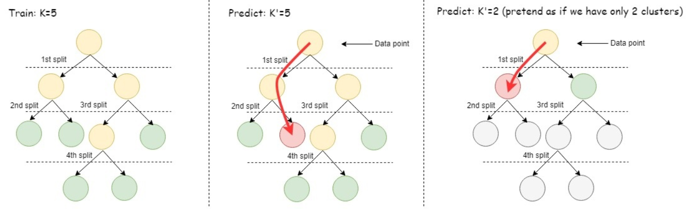
See also

• APPLY_BISECTING_KMEANS
• BISECTING_KMEANS
• GET_MODEL_SUMMARY

6 - Time series forecasting

Time series models are trained on stationary time series (that is, time series where the mean doesn't change over time) of stochastic processes with consistent time steps. These algorithms forecast future values by taking into account the influence of values at some number of preceding timesteps (lags).

Examples of applicable datasets include those for temperature, stock prices, earthquakes, product sales, etc.

To normalize datasets with inconsistent timesteps, see Gap filling and interpolation (GFI).

6.1 - ARIMA model example

Autoregressive integrated moving average (ARIMA) models combine the abilities of AUTOREGRESSOR and MOVING_AVERAGE models by making predictions based on both preceding time series values and errors of previous predictions. ARIMA models also provide the option to apply a differencing operation to the input data, which can turn a non-stationary time series into a stationary time series. At model training time, you specify the differencing order and the number of preceding values and previous prediction errors that the model uses to calculate predictions.

You can use the following functions to train and make predictions with ARIMA models:

• ARIMA: Creates and trains an ARIMA model

• PREDICT_ARIMA: Applies a trained ARIMA model to an input relation or makes predictions using the in-sample data

These functions require time series data with consistent timesteps. To normalize a time series with inconsistent timesteps, see Gap filling and interpolation (GFI).

The following example trains three ARIMA models, two that use differencing and one that does not, and then makes predictions using the models.

Load the training data

This example uses the following data:

• daily-min-temperatures: provided in the machine learning sample data, this dataset contains data on the daily minimum temperature in Melbourne, Australia from 1981 through 1990. After you load the sample datasets, this data is available in the temp_data table.
• db_size: a table that tracks the size of a database over consecutive months.

=> SELECT * FROM temp_data;
        time         | Temperature
---------------------+-------------
 1981-01-01 00:00:00 |        20.7
 1981-01-02 00:00:00 |        17.9
 1981-01-03 00:00:00 |        18.8
 1981-01-04 00:00:00 |        14.6
 1981-01-05 00:00:00 |        15.8
 ...
 1990-12-27 00:00:00 |          14
 1990-12-28 00:00:00 |        13.6
 1990-12-29 00:00:00 |        13.5
 1990-12-30 00:00:00 |        15.7
 1990-12-31 00:00:00 |          13
(3650 rows)

=> SELECT COUNT(*) FROM temp_data;
 COUNT
-------
3650
(1 row)

=> => SELECT * FROM db_size;
 month | GB
-------+-----
     1 |   5
     2 |  10
     3 |  20
     4 |  35
     5 |  55
     6 |  80
     7 | 110
     8 | 145
     9 | 185
    10 | 230
(10 rows)

Train the ARIMA models

After you load the daily-min-temperatures data, you can use the ARIMA function to create and train an ARIMA model. For this example, the model is trained with lags of p=3 and q=3, taking the value and prediction error of three previous time steps into account for each prediction. Because the input time series is stationary, you don't need to apply differencing to the data:

=> SELECT ARIMA('arima_temp', 'temp_data', 'temperature', 'time' USING PARAMETERS p=3, d=0, q=3);
                             ARIMA
--------------------------------------------------------------
Finished in 20 iterations.
3650 elements accepted, 0 elements rejected.

(1 row)

You can view a summary of the model with the GET_MODEL_SUMMARY function:

=> SELECT GET_MODEL_SUMMARY(USING PARAMETERS model_name='arima_temp');
               GET_MODEL_SUMMARY
-----------------------------------------------

============
coefficients
============
parameter| value
---------+--------
  phi_1  | 0.64189
  phi_2  | 0.46667
  phi_3  |-0.11777
 theta_1 |-0.05109
 theta_2 |-0.58699
 theta_3 |-0.15882


==============
regularization
==============
none

===============
timeseries_name
===============
temperature

==============
timestamp_name
==============
time

==============
missing_method
==============
linear_interpolation

===========
call_string
===========
ARIMA('public.arima_temp', 'temp_data', 'temperature', 'time' USING PARAMETERS p=3, d=0, q=3, missing='linear_interpolation', init_method='Zero', epsilon=1e-06, max_iterations=100);

===============
Additional Info
===============
       Name       | Value
------------------+--------
        p         |   3
        q         |   3
        d         |   0
       mean       |11.17775
      lambda      | 1.00000
mean_squared_error| 5.80490
rejected_row_count|   0
accepted_row_count|  3650

(1 row)

Examining the db_size table, it is clear that there is an upward trend to the database size over time. Each month the database size increases five more gigabytes than the increase in the previous month. This trend indicates the time series is non-stationary.

To account for this in the ARIMA model, you must difference the data by setting a non-zero d parameter value. For comparison, two ARIMA models are trained on this data, the first with a d value of one and the second with a d value of two:

=> SELECT ARIMA('arima_d1', 'db_size', 'GB', 'month' USING PARAMETERS p=2, d=1, q=2);
                                 ARIMA
------------------------------------------------------------------------
 Finished in 9 iterations.
 10 elements accepted, 0 elements rejected.

(1 row)

=> SELECT ARIMA('arima_d2', 'db_size', 'GB', 'month' USING PARAMETERS p=2, d=2, q=2);
                                 ARIMA
------------------------------------------------------------------------
 Finished in 0 iterations.
 10 elements accepted, 0 elements rejected.

(1 row)

Make predictions

After you train the ARIMA models, you can call the PREDICT_ARIMA function to predict future time series values. This function supports making predictions using the in-sample data that the models were trained on or applying the model to an input relation.

Using in-sample data

The following PREIDCT_ARIMA call makes temperature predictions using the in-sample data that the arima_temp model was trained on. The model begins prediction at the end of the temp_data table and returns predicted values for ten timesteps:

=> SELECT PREDICT_ARIMA(USING PARAMETERS model_name='arima_temp', start=0, npredictions=10) OVER();
   prediction
------------------
12.9745063293842
13.4389080858551
13.3955791360528
13.3551146487462
13.3149336514747
13.2750516811057
13.2354710353376
13.1961939790513
13.1572226788109
13.1185592045127
(10 rows)

For both prediction methods, if you want the function to return the standard error of each prediction, you can set output_standard_errors to true:

=> SELECT PREDICT_ARIMA(USING PARAMETERS model_name='arima_temp', start=0, npredictions=10, output_standard_errors=true) OVER();
    prediction    |     std_err
------------------+------------------
 12.9745063293842 | 1.00621890780865
 13.4389080858551 | 1.45340836833232
 13.3955791360528 | 1.61041524562932
 13.3551146487462 | 1.76368421116143
 13.3149336514747 | 1.91223938476627
 13.2750516811057 | 2.05618464609977
 13.2354710353376 | 2.19561771498385
 13.1961939790513 | 2.33063553781651
 13.1572226788109 | 2.46133422924445
 13.1185592045127 | 2.58780904243988
(10 rows)

To make predictions with the two models trained on the db_size table, you only need to change the specified model_name in the above calls:

=> SELECT PREDICT_ARIMA(USING PARAMETERS model_name='arima_d1', start=0, npredictions=10) OVER();
    prediction
------------------
 279.882778508943
 334.398317856829
 393.204492820962
 455.909453114272
 522.076165355683
 591.227478668175
 662.851655189833
 736.408301395412
 811.334631481162
 887.051990217688
(10 rows)

=> SELECT PREDICT_ARIMA(USING PARAMETERS model_name='arima_d2', start=0, npredictions=10) OVER();
 prediction
------------
        280
        335
        395
        460
        530
        605
        685
        770
        860
        955
(10 rows)

Comparing the outputs from the two models, you can see that the model trained with a d value of two correctly captures the trend in the data. Each month the rate of database growth increases by five gigabytes.

Applying to an input relation

You can also apply the model to an input relation. The following example makes predictions by applying the arima_temp model to the temp_data training set:

=> SELECT PREDICT_ARIMA(temperature USING PARAMETERS model_name='arima_temp', start=3651, npredictions=10, output_standard_errors=true) OVER(ORDER BY time) FROM temp_data;
    prediction    |     std_err
------------------+------------------
 12.9745063293842 | 1.00621890780865
 13.4389080858551 | 1.45340836833232
 13.3955791360528 | 1.61041524562932
 13.3551146487462 | 1.76368421116143
 13.3149336514747 | 1.91223938476627
 13.2750516811057 | 2.05618464609977
 13.2354710353376 | 2.19561771498385
 13.1961939790513 | 2.33063553781651
 13.1572226788109 | 2.46133422924445
 13.1185592045127 | 2.58780904243988
(10 rows)

Because the same data and relative start index were provided to both prediction methods, the arima_temp model predictions for each method are identical.

When applying a model to an input relation, you can set add_mean to false so that the function returns the predicted difference from the mean instead of the sum of the model mean and the predicted difference:

=> SELECT PREDICT_ARIMA(temperature USING PARAMETERS model_name='arima_temp', start=3680, npredictions=10, add_mean=false) OVER(ORDER BY time) FROM temp_data;
  prediction
------------------
1.2026877112171
1.17114068517961
1.13992534953432
1.10904183333367
1.0784901998692
1.04827044781798
1.01838251238116
0.98882626641461
0.959601521551628
0.93070802931751
(10 rows)

See also

• ARIMA
• PREDICT_ARIMA
• GET_MODEL_SUMMARY
• MSE

6.2 - Autoregressive model example

Autoregressive models predict future values of a time series based on the preceding values. More specifically, the user-specified lag determines how many previous timesteps it takes into account during computation, and predicted values are linear combinations of the values at each lag.

Use the following functions when training and predicting with autoregressive models. Note that these functions require datasets with consistent timesteps.

• AUTOREGRESSOR: trains an autoregressive model

• PREDICT_AUTOREGRESSOR: applies the model to a dataset to make predictions

To normalize datasets with inconsistent timesteps, see Gap filling and interpolation (GFI).

Example

1. Load the datasets from the Machine-Learning-Examples repository.

   This example uses the daily-min-temperatures dataset, which contains data on the daily minimum temperature in Melbourne, Australia from 1981 through 1990:

   => SELECT * FROM temp_data;
           time         | Temperature
   ---------------------+-------------
    1981-01-01 00:00:00 |        20.7
    1981-01-02 00:00:00 |        17.9
    1981-01-03 00:00:00 |        18.8
    1981-01-04 00:00:00 |        14.6
    1981-01-05 00:00:00 |        15.8
   ...
    1990-12-27 00:00:00 |          14
    1990-12-28 00:00:00 |        13.6
    1990-12-29 00:00:00 |        13.5
    1990-12-30 00:00:00 |        15.7
    1990-12-31 00:00:00 |          13
   (3650 rows)
   

2. Use AUTOREGRESSOR to create the autoregressive model AR_temperature from the temp_data dataset. In this case, the model is trained with a lag of p=3, taking the previous 3 entries into account for each estimation:

   => SELECT AUTOREGRESSOR('AR_temperature', 'temp_data', 'Temperature', 'time' USING PARAMETERS p=3);
                       AUTOREGRESSOR
   ---------------------------------------------------------
    Finished. 3650 elements accepted, 0 elements rejected.
   (1 row)
   

   You can view a summary of the model with GET_MODEL_SUMMARY:

   
   => SELECT GET_MODEL_SUMMARY(USING PARAMETERS model_name='AR_temperature');
   
    GET_MODEL_SUMMARY
   -------------------
   
   ============
   coefficients
   ============
   parameter| value
   ---------+--------
     alpha  | 1.88817
   phi_(t-1)| 0.70004
   phi_(t-2)|-0.05940
   phi_(t-3)| 0.19018
   
   
   ==================
   mean_squared_error
   ==================
   not evaluated
   
   ===========
   call_string
   ===========
   autoregressor('public.AR_temperature', 'temp_data', 'temperature', 'time'
   USING PARAMETERS p=3, missing=linear_interpolation, regularization='none', lambda=1, compute_mse=false);
   
   ===============
   Additional Info
   ===============
          Name       |Value
   ------------------+-----
       lag_order     |  3
   rejected_row_count|  0
   accepted_row_count|3650
   (1 row)
   

3. Use PREDICT_AUTOREGRESSOR to predict future temperatures. The following query starts the prediction at the end of the dataset and returns 10 predictions.

   => SELECT PREDICT_AUTOREGRESSOR(Temperature USING PARAMETERS model_name='AR_temperature', npredictions=10) OVER(ORDER BY time) FROM temp_data;
   
       prediction
   ------------------
    12.6235419917807
    12.9387860506032
    12.6683380680058
    12.3886937385419
    12.2689506237424
    12.1503023330142
    12.0211734746741
    11.9150531529328
    11.825870404008
    11.7451846722395
   (10 rows)
   

6.3 - Moving-average model example

Moving average models use the errors of previous predictions to make future predictions. More specifically, the user-specified lag determines how many previous predictions and errors it takes into account during computation.

Use the following functions when training and predicting with moving-average models. Note that these functions require datasets with consistent timesteps.

• MOVING_AVERAGE: trains a moving-average model

• PREDICT_MOVING_AVERAGE: applies the model to a dataset to make predictions

To normalize datasets with inconsistent timesteps, see Gap filling and interpolation (GFI).

Example

1. Load the datasets from the Machine-Learning-Examples repository.

   This example uses the daily-min-temperatures dataset, which contains data on the daily minimum temperature in Melbourne, Australia from 1981 through 1990:

   => SELECT * FROM temp_data;
           time         | Temperature
   ---------------------+-------------
    1981-01-01 00:00:00 |        20.7
    1981-01-02 00:00:00 |        17.9
    1981-01-03 00:00:00 |        18.8
    1981-01-04 00:00:00 |        14.6
    1981-01-05 00:00:00 |        15.8
   ...
    1990-12-27 00:00:00 |          14
    1990-12-28 00:00:00 |        13.6
    1990-12-29 00:00:00 |        13.5
    1990-12-30 00:00:00 |        15.7
    1990-12-31 00:00:00 |          13
   (3650 rows)
   

2. Use MOVING_AVERAGE to create the moving-average model MA_temperature from the temp_data dataset. In this case, the model is trained with a lag of p=3, taking the error of 3 previous predictions into account for each estimation:

   => SELECT MOVING_AVERAGE('MA_temperature', 'temp_data', 'temperature', 'time' USING PARAMETERS q=3, missing='linear_interpolation', regularization='none', lambda=1);
                       MOVING_AVERAGE
   ---------------------------------------------------------
    Finished. 3650 elements accepted, 0 elements rejected.
   (1 row)
   

   You can view a summary of the model with GET_MODEL_SUMMARY:

   
   => SELECT GET_MODEL_SUMMARY(USING PARAMETERS model_name='MA_temperature');
   
    GET_MODEL_SUMMARY
   -------------------
   
   ============
   coefficients
   ============
   parameter| value
   ---------+--------
   phi_(t-0)|-0.90051
   phi_(t-1)|-0.10621
   phi_(t-2)| 0.07173
   
   
   ===============
   timeseries_name
   ===============
   temperature
   
   ==============
   timestamp_name
   ==============
   time
   
   ===========
   call_string
   ===========
   moving_average('public.MA_temperature', 'temp_data', 'temperature', 'time'
   USING PARAMETERS q=3, missing=linear_interpolation, regularization='none', lambda=1);
   
   ===============
   Additional Info
   ===============
          Name       | Value
   ------------------+--------
          mean       |11.17780
       lag_order     |   3
         lambda      | 1.00000
   rejected_row_count|   0
   accepted_row_count|  3650
   
   (1 row)
   

3. Use PREDICT_MOVING_AVERAGE to predict future temperatures. The following query starts the prediction at the end of the dataset and returns 10 predictions.

   => SELECT PREDICT_MOVING_AVERAGE(Temperature USING PARAMETERS model_name='MA_temperature', npredictions=10) OVER(ORDER BY time) FROM temp_data;
   
       prediction
   ------------------
    13.1324365636272
    12.8071086272833
    12.7218966671721
    12.6011086656032
    12.506624729879
    12.4148247026733
    12.3307873804812
    12.2521385975133
    12.1789741993396
    12.1107640076638
   (10 rows)
   

7 - Model management

Vertica provides a number of tools to manage existing models. You can view model summaries and attributes, alter model characteristics like name and privileges, drop models, and version models.

7.1 - Model versioning

Model versioning provides an infrastructure to track and manage the status of registered models in a database. The versioning infrastructure supports a collaborative environment where multiple users can submit candidate models for individual applications, which are identified by their registered_name. Models in Vertica are by default unregistered, but any user with sufficient privileges can register a model to an application and add it to the versioning environment.

Register models

When a candidate model is ready to be submitted to an application, the model owner or any user with sufficient privileges, including any user with the DBADMIN or MLSUPERVISOR role, can register the model using the REGISTER_MODEL function. The registered model is assigned an initial status of 'under_review' and is visible in the REGISTERED_MODELS system table to users with USAGE privileges.

All registered models under a given registered_name are considered different versions of the same model, regardless of trainer, algorithm type, or production status. If a model is the first to be registered to a given registered_name, the model is assigned a registered_version of one. Otherwise, newly registered models are assigned an incremented registered_version of n + 1, where n is the number of models already registered to the given registered_name. Each registered model can be uniquely identified by the combination of registered_name and registered_version.

Change model status

After a model is registered, the model owner is automatically changed to superuser and the previous owner is given USAGE privileges. The MLSUPERVISOR role has full privileges over all registered models, as does dbadmin. Only users with these two roles can call the CHANGE_MODEL_STATUS function to change the status of registered models. There are six possible statuses for registered models:

• under_review: Status assigned to newly registered models.

• staging: Model is targeted for A/B testing against the model currently in production.

• production: Model is in production for its specified application. Only one model can be in production for a given registered_name at one time.

• archived: Status of models that were previously in production. Archived models can be returned to production at any time.

• declined: Model is no longer in consideration for production.

• unregistered: Model is removed from the versioning environment. The model does not appear in the REGISTERED_MODELS system table.

The following diagram depicts the valid status transitions:

You can view the status history of registered models with the MODEL_STATUS_HISTORY system table, which includes models that have been unregistered or dropped. Only superusers or users to whom they have granted sufficient privileges can query the table. Vertica recommends granting access on the table to the MLSUPERVISOR role.

Managing registered models

Only users with the MLSUPERVISOR role, or those granted equivalent privileges, can drop or alter registered models. As with unregistered models, you can drop and alter registered models with the DROP MODEL and ALTER MODEL commands. Dropped models no longer appear in the REGISTERED_MODELS system table.

To make predictions with a registered model, you must use the [schema_name.]model_name and predict function for the appropriate model type. You can find all necessary information in the REGISTERED_MODELS system table.

Model registration does not effect the process of exporting models. However, model registration information, such as registered_version, is not captured in exported models. All imported models are initially unregistered, but each category of imported model—native Vertica, PMML, and TensorFlow—is compatible with model versioning.

Examples

The following example demonstrates a possible model versioning workflow. This workflow begins with registering multiple models to an application, continues with an MLSUPERVISOR managing and changing the status of those models, and concludes with one of the models in production.

First, the models must be registered to an application. In this case, the models, native_linear_reg and linear_reg_spark1, are registered as the linear_reg_app application:

=> SELECT REGISTER_MODEL('native_linear_reg', 'linear_reg_app');
                           REGISTER_MODEL
-------------------------------------------------------------------------
Model [native_linear_reg] is registered as [linear_reg_app], version [2]
(1 row)

=> SELECT REGISTER_MODEL('linear_reg_spark1', 'linear_reg_app');
                           REGISTER_MODEL
-------------------------------------------------------------------------
Model [linear_reg_spark1] is registered as [linear_reg_app], version [3]
(1 row)

You can query the REGISTERED_MODELS system table to view details about the newly registered models, such as the version number and model status:

=> SELECT * FROM REGISTERED_MODELS;
  registered_name | registered_version |    status    |        registered_time        |      model_id     | schema_name |    model_name     |      model_type       |    category
------------------+--------------------+--------------+-------------------------------+-------------------+-------------+-------------------+-----------------------+----------------
 linear_reg_app   |                  3 | UNDER_REVIEW | 2023-01-26 09:52:00.082166-04 | 45035996273714020 | public      | linear_reg_spark1 | PMML_REGRESSION_MODEL | PMML
 linear_reg_app   |                  2 | UNDER_REVIEW | 2023-01-26 09:51:04.553102-05 | 45035996273850350 | public      | native_linear_reg | LINEAR_REGRESSION     | VERTICA_MODELS
 linear_reg_app   |                  1 | PRODUCTION   | 2023-01-24 05:29:25.990626-02 | 45035996273853740 | public      | linear_reg_newton | LINEAR_REGRESSION     | VERTICA_MODELS
 logistic_reg_app |                  1 | PRODUCTION   | 2023-01-23 08:49:25.990626-02 | 45035996273853740 | public      | log_reg_cgd       | LOGISTIC_REGRESSION   | VERTICA_MODELS
(4 rows)

If you query the MODELS system table, you can see that the model owner has automatically been changed to superuser, dbadmin in this case:

=> SELECT model_name, owner_name FROM MODELS WHERE model_name IN ('native_linear_reg', 'linear_reg_spark1');
     model_name    | owner_name
-------------------+------------
 native_linear_reg | dbadmin
 linear_reg_spark1 | dbadmin
(2 rows)

As a user with the MLSUPERVISOR role enabled, you can then change the status of both models to 'staging' with the CHANGE_MODEL_STATUS function, which accepts a registered_name and registered_version:

=> SELECT CHANGE_MODEL_STATUS('linear_reg_app', 2, 'staging');
                          CHANGE_MODEL_STATUS
-----------------------------------------------------------------------------
The status of model [linear_reg_app] - version [2] is changed to [staging]
(1 row)

=> SELECT CHANGE_MODEL_STATUS('linear_reg_app', 3, 'staging');
                          CHANGE_MODEL_STATUS
-----------------------------------------------------------------------------
The status of model [linear_reg_app] - version [3] is changed to [staging]
(1 row)

After comparing the evaluation metrics of the two staged models against the model currently in production, you can put the better performing model into production. In this case, the linear_reg_spark1 model is moved into production and the linear_reg_spark1 model is declined:

=> SELECT CHANGE_MODEL_STATUS('linear_reg_app', 2, 'declined');
CHANGE_MODEL_STATUS
-----------------------------------------------------------------------------
The status of model [linear_reg_app] - version [2] is changed to [declined]
(1 row)

=> SELECT CHANGE_MODEL_STATUS('linear_reg_app', 3, 'production');
CHANGE_MODEL_STATUS
-----------------------------------------------------------------------------
The status of model [linear_reg_app] - version [3] is changed to [production]
(1 row)

You can then query the REGISTERED_MODELS system table to confirm that the linear_reg_spark1 model is now in 'production', the native_linear_reg model has been set to 'declined', and the previously in production linear_reg_spark1 model has been automatically moved to 'archived':

=> SELECT * FROM REGISTERED_MODELS;
  registered_name | registered_version |    status    |        registered_time        |      model_id     | schema_name |    model_name     |      model_type       |    category
------------------+--------------------+--------------+-------------------------------+-------------------+-------------+-------------------+-----------------------+----------------
 linear_reg_app   |                  3 | PRODUCTION   | 2023-01-26 09:52:00.082166-04 | 45035996273714020 | public      | linear_reg_spark1 | PMML_REGRESSION_MODEL | PMML
 linear_reg_app   |                  2 | DECLINED     | 2023-01-26 09:51:04.553102-05 | 45035996273850350 | public      | native_linear_reg | LINEAR_REGRESSION     | VERTICA_MODELS
 linear_reg_app   |                  1 | ARCHIVED     | 2023-01-24 05:29:25.990626-02 | 45035996273853740 | public      | linear_reg_newton | LINEAR_REGRESSION     | VERTICA_MODELS
 logistic_reg_app |                  1 | PRODUCTION   | 2023-01-23 08:49:25.990626-02 | 45035996273853740 | public      | log_reg_cgd       | LOGISTIC_REGRESSION   | VERTICA_MODELS
(4 rows)

To remove the declined native_linear_reg model from the versioning environment, you can set the status to 'unregistered':

=> SELECT CHANGE_MODEL_STATUS('linear_reg_app', 2, 'unregistered');
                            CHANGE_MODEL_STATUS
----------------------------------------------------------------------------------
The status of model [linear_reg_app] - version [2] is changed to [unregistered]
(1 row)

=> SELECT * FROM REGISTERED_MODELS;
  registered_name | registered_version |    status    |        registered_time        |      model_id     | schema_name |    model_name     |      model_type       |    category
------------------+--------------------+--------------+-------------------------------+-------------------+-------------+-------------------+-----------------------+----------------
 linear_reg_app   |                  3 | PRODUCTION   | 2023-01-26 09:52:00.082166-04 | 45035996273714020 | public      | linear_reg_spark1 | PMML_REGRESSION_MODEL | PMML
 linear_reg_app   |                  1 | ARCHIVED     | 2023-01-24 05:29:25.990626-02 | 45035996273853740 | public      | linear_reg_newton | LINEAR_REGRESSION     | VERTICA_MODELS
 logistic_reg_app |                  1 | PRODUCTION   | 2023-01-23 08:49:25.990626-02 | 45035996273853740 | public      | log_reg_cgd       | LOGISTIC_REGRESSION   | VERTICA_MODELS
(3 rows)

You can see that the native_linear_reg model no longer appears in the REGISTERED_MODELS system table. However, you can still query the MODEL_STATUS_HISTORY system table to view the status history of native_linear_reg:

=> SELECT * FROM MODEL_STATUS_HISTORY WHERE model_id=45035996273850350;
 registered_name | registered_version |  new_status  |  old_status  |       status_change_time      |    operator_id    | operator_name |      model_id     | schema_name |    model_name
-----------------+--------------------+--------------+------------- +-------------------------------+-------------------+---------------+-------------------+-------------+-------------------
linear_reg_app   |                  2 | UNDER_REVIEW | UNREGISTERED | 2023-01-26 09:51:04.553102-05 | 45035996273964824 | user1         | 45035996273850350 | public      | native_linear_reg
linear_reg_app   |                  2 | STAGING      | UNDER_REVIEW | 2023-01-29 11:33:02.052464-05 | 45035996273704962 | supervisor1   | 45035996273850350 | public      | native_linear_reg
linear_reg_app   |                  2 | DECLINED     | STAGING      | 2023-01-30 04:12:30.481136-05 | 45035996273704962 | supervisor1   | 45035996273850350 | public      | native_linear_reg
linear_reg_app   |                  2 | UNREGISTERED | DECLINED     | 2023-02-02 03:25:32.332132-05 | 45035996273704962 | supervisor1   | 45035996273850350 | public      | native_linear_reg
(4 rows)

See also

• REGISTERED_MODELS
• MODEL_STATUS_HISTORY
• REGISTER_MODEL
• CHANGE_MODEL_STATUS
• MLSUPERVISOR

7.2 - Altering models

You can modify a model using ALTER MODEL, in response to your model's needs. You can alter a model by renaming the model, changing the owner, and changing the schema.

You can drop or alter any model that you create.

7.2.1 - Changing model ownership

As a superuser or model owner, you can reassign model ownership with ALTER MODEL as follows:

ALTER MODEL model-nameOWNER TOowner-name

Changing model ownership is useful when a model owner leaves or changes responsibilities. Because you can change the owner, the models do not need to be rewritten.

Example

The following example shows how you can use ALTER_MODEL to change the model owner:

1. Find the model you want to alter. As the dbadmin, you own the model.

   => SELECT * FROM V_CATALOG.MODELS WHERE model_name='mykmeansmodel';
   -[ RECORD 1 ]--+------------------------------------------
   model_id       | 45035996273816618
   model_name     | mykmeansmodel
   schema_id      | 45035996273704978
   schema_name    | public
   owner_id       | 45035996273704962
   owner_name     | dbadmin
   category       | VERTICA_MODELS
   model_type     | kmeans
   is_complete    | t
   create_time    | 2017-03-02 11:16:04.990626-05
   size           | 964
   

2. Change the model owner from dbadmin to user1.

   => ALTER MODEL mykmeansmodel OWNER TO user1;
        ALTER MODEL
   

3. Review V_CATALOG.MODELS to verify that the owner was changed.

   => SELECT * FROM V_CATALOG.MODELS WHERE model_name='mykmeansmodel';
   
   -[ RECORD 1 ]--+------------------------------------------
   model_id       | 45035996273816618
   model_name     | mykmeansmodel
   schema_id      | 45035996273704978
   schema_name    | public
   owner_id       | 45035996273704962
   owner_name     | user1
   category       | VERTICA_MODELS
   model_type     | kmeans
   is_complete    | t
   create_time    | 2017-03-02 11:16:04.990626-05
   size           | 964
   

7.2.2 - Moving models to another schema

You can move a model from one schema to another with ALTER MODEL. You can move the model as a superuser or user with USAGE privileges on the current schema and CREATE privileges on the destination schema.

Example

The following example shows how you can use ALTER MODEL to change the model schema:

1. Find the model you want to alter.

   => SELECT * FROM V_CATALOG.MODELS WHERE model_name='mykmeansmodel';
   -[ RECORD 1 ]--+------------------------------------------
   model_id       | 45035996273816618
   model_name     | mykmeansmodel
   schema_id      | 45035996273704978
   schema_name    | public
   owner_id       | 45035996273704962
   owner_name     | dbadmin
   category       | VERTICA_MODELS
   model_type     | kmeans
   is_complete    | t
   create_time    | 2017-03-02 11:16:04.990626-05
   size           | 964
   

2. Change the model schema.

   => ALTER MODEL mykmeansmodel SET SCHEMA test;
        ALTER MODEL
   

3. Review V_CATALOG.MODELS to verify that the owner was changed.

   => SELECT * FROM V_CATALOG.MODELS WHERE model_name='mykmeansmodel';
   
   -[ RECORD 1 ]--+------------------------------------------
   model_id       | 45035996273816618
   model_name     | mykmeansmodel
   schema_id      | 45035996273704978
   schema_name    | test
   owner_id       | 45035996273704962
   owner_name     | dbadmin
   category       | VERTICA_MODELS
   model_type     | kmeans
   is_complete    | t
   create_time    | 2017-03-02 11:16:04.990626-05
   size           | 964
   

7.2.3 - Renaming a model

ALTER MODEL lets you rename models. For example:

1. Find the model you want to alter.

   => SELECT * FROM V_CATALOG.MODELS WHERE model_name='mymodel';
   -[ RECORD 1 ]--+------------------------------------------
   model_id       | 45035996273816618
   model_name     | mymodel
   schema_id      | 45035996273704978
   schema_name    | public
   owner_id       | 45035996273704962
   owner_name     | dbadmin
   category       | VERTICA_MODELS
   model_type     | kmeans
   is_complete    | t
   create_time    | 2017-03-02 11:16:04.990626-05
   size           | 964
   

2. Rename the model.

   => ALTER MODEL mymodel RENAME TO mykmeansmodel;
        ALTER MODEL
   

3. Review V_CATALOG.MODELS to verify that the model name was changed.

   => SELECT * FROM V_CATALOG.MODELS WHERE model_name='mykmeansmodel';
   
   -[ RECORD 1 ]--+------------------------------------------
   model_id       | 45035996273816618
   model_name     | mykmeansmodel
   schema_id      | 45035996273704978
   schema_name    | public
   owner_id       | 45035996273704962
   owner_name     | dbadmin
   category       | VERTICA_MODELS
   model_type     | kmeans
   is_complete    | t
   create_time    | 2017-03-02 11:16:04.990626-05
   size           | 964
   

7.3 - Dropping models

DROP MODEL removes one or more models from the database. For example:

1. Find the model you want to drop.

   => SELECT * FROM V_CATALOG.MODELS WHERE model_name='mySvmClassModel';
   -[ RECORD 1 ]--+--------------------------------
   model_id       | 45035996273765414
   model_name     | mySvmClassModel
   schema_id      | 45035996273704978
   schema_name    | public
   owner_id       | 45035996273704962
   owner_name     | dbadmin
   category       | VERTICA_MODELS
   model_type     | SVM_CLASSIFIER
   is_complete    | t
   create_time    | 2017-02-14 10:30:44.903946-05
   size           | 525
   

2. Drop the model.

   => DROP MODEL mySvmClassModel;
        DROP MODEL
   

3. Review V_CATALOG.MODELS to verify that the model was dropped.

   => SELECT * FROM V_CATALOG.MODELS WHERE model_name='mySvmClassModel';
   (0 rows)
   

7.4 - Managing model security

You can manage the security privileges on your models by using the GRANT and REVOKE statements. The following examples show how you can change privileges on user1 and user2 using the faithful table and the linearReg model.

• In the following example, the dbadmin grants the SELECT privilege to user1:

  => GRANT SELECT ON TABLE faithful TO user1;
  GRANT PRIVILEGE
  

• Then, the dbadmin grants the CREATE privilege on the public schema to user1:

  => GRANT CREATE ON SCHEMA public TO user1;
  GRANT PRIVILEGE
  

• Connect to the database as user1:

  => \c - user1
  

• As user1, build the linearReg model:

=> SELECT LINEAR_REG('linearReg', 'faithful', 'waiting', 'eruptions');
LINEAR_REG
---------------------------
Finished in 1 iterations
(1 row)

• As user1, grant USAGE privileges to user2:

=> GRANT USAGE ON MODEL linearReg TO user2;
GRANT PRIVILEGE

• Connect to the database as user2:

=> \c - user2

• To confirm privileges were granted to user2, run the GET_MODEL_SUMMARY function. A user with the USAGE privilege on a model can run GET_MODEL_SUMMARY on that model:

=> SELECT GET_MODEL_SUMMARY(USING PARAMETERS model_name='linearReg');

=======
details
=======
predictor|coefficient|std_err |t_value |p_value
---------+-----------+--------+--------+--------
Intercept| 33.47440  | 1.15487|28.98533| 0.00000
eruptions| 10.72964  | 0.31475|34.08903| 0.00000

==============
regularization
==============
type| lambda
----+--------
none| 1.00000

===========
call_string
===========
linear_reg('public.linearReg', 'faithful', '"waiting"', 'eruptions'
USING PARAMETERS optimizer='newton', epsilon=1e-06, max_iterations=100, regularization='none', lambda=1)

===============
Additional Info
===============
Name              |Value
------------------+-----
iteration_count   |  1
rejected_row_count|  0
accepted_row_count| 272
(1 row)

• Connect to the database as user1:

=> \c - user1

• Then, you can use the REVOKE statement to revoke privileges from user2:

=> REVOKE USAGE ON MODEL linearReg FROM user2;
REVOKE PRIVILEGE

• To confirm the privileges were revoked, connect as user 2 and run the GET_MODEL_SUMMARY function:

=> \c - user2
=>SELECT GET_MODEL_SUMMARY('linearReg');
ERROR 7523:  Problem in get_model_summary.
Detail: Permission denied for model linearReg

See also

• GRANT (model)
• REVOKE (model)

7.5 - Viewing model attributes

The following topics explain the model attributes for the Vertica machine learning algorithms. These attributes describe the internal structure of a particular model:

• Cross validation model attributes

• K-means model attributes

• Naive Bayes model attributes

• Normalization model attributes

• One Hot Encoder model attributes

• Random forest model attributes

• Regression model attributes

• SVM model attributes

7.6 - Summarizing models

1. Find the model you want to summarize.

   => SELECT * FROM v_catalog.models WHERE model_name='svm_class';
   model_id      | model_name |     schema_id   | schema_name |     owner_id      | owner_name |    category    |
   model_type   | is_complete |     create_time          | size
   -------------------+------------+-------------------+-------------+-------------------+------------+--------
   --------+----------------+-------------+-------------------------------+------
   45035996273715226 | svm_class  | 45035996273704980 | public      | 45035996273704962 | dbadmin    | VERTICA_MODELS
   | SVM_CLASSIFIER | t           | 2017-08-28 09:49:00.082166-04 | 1427
   (1 row)
   

2. View the model summary.

   
   => SELECT GET_MODEL_SUMMARY(USING PARAMETERS model_name='svm_class');
   ------------------------------------------------------------------------
   
   =======
   details
   =======
   predictor|coefficient
   ---------+-----------
   Intercept| -0.02006
   cyl      |  0.15367
   mpg      |  0.15698
   wt       | -1.78157
   hp       |  0.00957
   
   ===========
   call_string
   ===========
   SELECT svm_classifier('public.svm_class', 'mtcars_train', '"am"', 'cyl, mpg, wt, hp, gear'
   USING PARAMETERS exclude_columns='gear', C=1, max_iterations=100, epsilon=0.001);
   
   ===============
   Additional Info
   ===============
   Name              |Value
   ------------------+-----
   accepted_row_count| 20
   rejected_row_count|  0
   iteration_count   | 12
   (1 row)
   

See also

• GET_MODEL_SUMMARY

7.7 - Viewing models

Vertica stores the models you create in the V_CATALOG.MODELS system table.

You can query V_CATALOG.MODELS to view information about the models you have created:

=> SELECT * FROM V_CATALOG.MODELS;
-[ RECORD 1 ]--+------------------------------------------
model_id       | 45035996273765414
model_name     | mySvmClassModel
schema_id      | 45035996273704978
schema_name    | public
owner_id       | 45035996273704962
owner_name     | dbadmin
category       | VERTICA_MODELS
model_type     | SVM_CLASSIFIER
is_complete    | t
create_time    | 2017-02-14 10:30:44.903946-05
size           | 525
-[ RECORD 2 ]--+------------------------------------------

model_id       | 45035996273711466
model_name     | mtcars_normfit
schema_id      | 45035996273704978
schema_name    | public
owner_id       | 45035996273704962
owner_name     | dbadmin
category       | VERTICA_MODELS
model_type     | SVM_CLASSIFIER
is_complete    | t
create_time    | 2017-02-06 15:03:05.651941-05
size           | 288

See also

• MODELS
• V_CATALOG schema

8 - Using external models with Vertica

To give you the utmost in machine learning flexibility and scalability, Vertica supports importing, exporting, and predicting with PMML and TensorFlow models.

The machine learning configuration parameter MaxModelSizeKB sets the maximum size of a model that can be imported into Vertica.

Support for PMML models

Vertica supports the import and export of machine learning models in Predictive Model Markup Language (PMML) format. Support for this platform-independent model format allows you to use models trained on other platforms to predict on data stored in your Vertica database. You can also use Vertica as your model repository. Vertica supports PMML version 4.4.1.

With the PREDICT_PMML function, you can use a PMML model archived in Vertica to run prediction on data stored in the Vertica database. For more information, see Using PMML models.

For details on the PMML models, tags, and attributes that Vertica supports, see PMML features and attributes.

Support for TensorFlow models

Vertica now supports importing trained TensorFlow models, and using those models to do prediction in Vertica on data stored in the Vertica database. Vertica supports TensorFlow models trained in TensorFlow version 1.15.

The PREDICT_TENSORFLOW and PREDICT_TENSORFLOW_SCALAR functions let you predict on data in Vertica with TensorFlow models.

For additional information, see TensorFlow models.

Additional external model support

The following functions support both PMML and TensorFlow models:

• IMPORT_MODELS
• EXPORT_MODELS
• GET_MODEL_ATTRIBUTE
• GET_MODEL_SUMMARY

8.1 - TensorFlow models

Tensorflow is a framework for creating neural networks. It implements basic linear algebra and multi-variable calculus operations in a scalable fashion, and allows users to easily chain these operations into a computation graph.

Vertica supports importing, exporting, and making predictions with TensorFlow 1.x and 2.x models trained outside of Vertica.

In-database TensorFlow integration with Vertica offers several advantages:

• Your models live inside your database, so you never have to move your data to make predictions.

• The volume of data you can handle is limited only by the size of your Vertica database, which makes Vertica particularly well-suited for machine learning on Big Data.

• Vertica offers in-database model management, so you can store as many models as you want.

• Imported models are portable and can be exported for use elsewhere.

When you run a TensorFlow model to predict on data in the database, Vertica calls a TensorFlow process to run the model. This allows Vertica to support any model you can create and train using TensorFlow. Vertica just provides the inputs - your data in the Vertica database - and stores the outputs.

8.1.1 - TensorFlow integration and directory structure

This page covers importing Tensorflow models into Vertica, making predictions on data in the Vertica database, and exporting the model for use on another Vertica cluster or a third-party platform.

For a start-to-finish example through each operation, see TensorFlow example.

Vertica supports models created with either TensorFlow 1.x and 2.x, but 2.x is strongly recommended.

To use TensorFlow with Vertica, install the TFIntegration UDX package on any node. You only need to do this once:

$ /opt/vertica/bin/admintools -t install_package -d database_name -p 'password' --package TFIntegration

Directory and file structure for TensorFlow models

Before importing your models, you should have a separate directory for each model that contains each of the following files. Note that Vertica uses the directory name as the model name when you import it:

• model_name.pb: a trained model in frozen graph format

• tf_model_desc.json: a description of the model

For example, a tf_models directory that contains two models, tf_mnist_estimator and tf_mnist_keras, has the following layout:

tf_models/
├── tf_mnist_estimator
│   ├── mnist_estimator.pb
│   └── tf_model_desc.json
└── tf_mnist_keras
    ├── mnist_keras.pb
    └── tf_model_desc.json

You can generate both of these files for a given TensorFlow 2 (TF2) model with the freeze_tf2_model.py script included in the Machine-Learning-Examples GitHub repository and in the opt/vertica/packages/TFIntegration/examples directory in the Vertica database. The script accepts three arguments:

model-path

Path to a saved TF2 model directory.

folder-name

(Optional) Name of the folder to which the frozen model is saved; by default, frozen_tfmodel.

column-type

(Optional) Integer, either 0 or 1, that signifies whether the input and output columns for the model are primitive or complex types. Use a value of 0 (default) for primitive types, or 1 for complex.

For example, the following call outputs the frozen tf_autoencoder model, which accepts complex input/output columns, into the frozen_autoencoder folder:

$ python3 ./freeze_tf2_model.py path/to/tf_autoencoder frozen_autoencoder 1

tf_model_desc.json

The tf_model_desc.json file forms the bridge between TensorFlow and Vertica. It describes the structure of the model so that Vertica can correctly match up its inputs and outputs to input/output tables.

Notice that the freeze_tf2_model.py script automatically generates this file for your TensorFlow 2 model, and this generated file can often be used as-is. For more complex models or use cases, you might have to edit this file. For a detailed breakdown of each field, see tf_model_desc.json overview.

Importing TensorFlow models into Vertica

To import TensorFlow models, use IMPORT_MODELS with the category 'TENSORFLOW'.

Import a single model. Keep in mind that the Vertica database uses the directory name as the model name:

select IMPORT_MODELS ( '/path/tf_models/tf_mnist_keras' USING PARAMETERS category='TENSORFLOW');
 import_models
---------------
 Success
(1 row)

Import all models in the directory (where each model has its own directory) with a wildcard (*):

select IMPORT_MODELS ('/path/tf_models/*' USING PARAMETERS category='TENSORFLOW');
 import_models
---------------
 Success
(1 row)

Make predictions with an imported TensorFlow model

After importing your TensorFlow model, you can use the model to predict on data in a Vertica table. Vertica provides two functions for making predictions with imported TensorFlow models: PREDICT_TENSORFLOW and PREDICT_TENSORFLOW_SCALAR.

The function you choose depends on whether you specified a column-type of 0 or 1 when calling the freeze_tf2_model.py script. If column-type was 0, meaning the model accepts primitive input and output types, use PREDICT_TENSORFLOW to make predictions; otherwise, use PREDICT_TENSORFLOW_SCALAR, as your model should accept complex input and output types.

Using PREDICT_TENSORFLOW

The PREDICT_TENSORFLOW function is different from the other predict functions in that it does not accept any parameters that affect the input columns such as "exclude_columns" or "id_column"; rather, the function always predicts on all the input columns provided. However, it does accept a num_passthru_cols parameter which allows the user to "skip" some number of input columns, as shown below.

The OVER(PARTITION BEST) clause tells Vertica to parallelize the operation across multiple nodes. See Window partition clause for details:

=> select PREDICT_TENSORFLOW (*
                   USING PARAMETERS model_name='tf_mnist_keras', num_passthru_cols=1)
                   OVER(PARTITION BEST) FROM tf_mnist_test_images;

--example output, the skipped columns are displayed as the first columns of the output
 ID | col0 | col1 | col2 | col3 | col4 | col5 | col6 | col7 | col8 | col9
----+------+------+------+------+------+------+------+------+------+------
  1 |    0 |    0 |    1 |    0 |    0 |    0 |    0 |    0 |    0 |    0
  3 |    1 |    0 |    0 |    0 |    0 |    0 |    0 |    0 |    0 |    0
  6 |    0 |    0 |    0 |    0 |    1 |    0 |    0 |    0 |    0 |    0
...

Using PREDICT_TENSORFLOW_SCALAR

The PREDICT_TENSORFLOW_SCALAR function accepts one input column of type ROW, where each field corresponds to an input tensor. It returns one output column of type ROW, where each field corresponds to an output tensor. This complex type support can simplify the process for making predictions on data with many input features.

For instance, the MNIST handwritten digit classification dataset contains 784 input features for each input row, one feature for each pixel in the images of handwritten digits. The PREDICT_TENSORFLOW function requires that each of these input features are contained in a separate input column. By encapsulating these features into a single ARRAY, the PREDICT_TENSORFLOW_SCALAR function only needs a single input column of type ROW, where the pixel values are the array elements for an input field:

--Each array for the "image" field has 784 elements. 
=> SELECT * FROM mnist_train;
id |                   inputs
---+---------------------------------------------
 1 | {"image":[0, 0, 0,..., 244, 222, 210,...]}
 2 | {"image":[0, 0, 0,..., 185, 84, 223,...]}
 3 | {"image":[0, 0, 0,..., 133, 254, 78,...]}
 ...

In this case, the function output consists of a single opeartion with one tensor. The value of this field is an array of ten elements, which are all zero except for the element whose index is the predicted digit:

=> SELECT id, PREDICT_TENSORFLOW_SCALAR(inputs USING PARAMETERS model_name='tf_mnist_ct') FROM mnist_test;
 id |                   PREDICT_TENSORFLOW_SCALAR                      
----+-------------------------------------------------------------------
  1 | {"prediction:0":["0", "0", "0", "0", "1", "0", "0", "0", "0", "0"]} 
  2 | {"prediction:0":["0", "1", "0", "0", "0", "0", "0", "0", "0", "0"]} 
  3 | {"prediction:0":["0", "0", "0", "0", "0", "0", "0", "1", "0", "0"]} 
...

Exporting TensorFlow models

Vertica exports the model as a frozen graph, which can then be re-imported at any time. Keep in mind that models that are saved as a frozen graph cannot be trained further.

Use EXPORT_MODELS to export TensorFlow models. For example, to export the tf_mnist_keras model to the /path/to/export/to directory:

=> SELECT EXPORT_MODELS ('/path/to/export/to', 'tf_mnist_keras');
 export_models
---------------
 Success
(1 row)

When you export a TensorFlow model, the Vertica database creates and uses the specified directory to store files that describe the model:

$ ls tf_mnist_keras/
crc.json  metadata.json  mnist_keras.pb  model.json  tf_model_desc.json

The .pb and tf_model_desc.json files describe the model, and the rest are organizational files created by the Vertica database.

See also

• TensorFlow models
• TensorFlow example
• IMPORT_MODELS
• EXPORT_MODELS
• PREDICT_TENSORFLOW

8.1.2 - TensorFlow example

Vertica uses the TFIntegration UDX package to integrate with TensorFlow. You can train your models outside of your Vertica database, then import them to Vertica and make predictions on your data.

TensorFlow scripts and datasets are included in the GitHub repository under Machine-Learning-Examples/TensorFlow.

The example below creates a Keras (a TensorFlow API) neural network model trained on the MNIST handwritten digit classification dataset, the layers of which are shown below.

The data is fed through each layer from top to bottom, and each layer modifies the input before returning a score. In this example, the data passed in is a set of images of handwritten Arabic numerals and the output would be the probability of the input image being a particular digit:

inputs = keras.Input(shape=(28, 28, 1), name="image")
x = layers.Conv2D(32, 5, activation="relu")(inputs)
x = layers.MaxPooling2D(2)(x)
x = layers.Conv2D(64, 5, activation="relu")(x)
x = layers.MaxPooling2D(2)(x)
x = layers.Flatten()(x)
x = layers.Dense(10, activation='softmax', name='OUTPUT')(x)
tfmodel = keras.Model(inputs, x)

For more information on how TensorFlow interacts with your Vertica database and how to import more complex models, see TensorFlow integration and directory structure.

Prepare a TensorFlow model for Vertica

The following procedures take place outside of Vertica.

Train and save a TensorFlow model

1. Install TensorFlow 2.

2. Train your model. For this particular example, you can run train_simple_model.py to train and save the model. Otherwise, and more generally, you can manually train your model in Python and then save it:

   $ mymodel.save('my_saved_model_dir')
   

3. Run the freeze_tf2_model.py script included in the Machine-Learning-Examples repository or in opt/vertica/packages/TFIntegration/examples, specifying your model, an output directory (optional, defaults to frozen_tfmodel), and the input and output column type (0 for primitive, 1 for complex).

   This script transforms your saved model into the Vertica-compatible frozen graph format and creates the tf_model_desc.json file, which describes how Vertica should translate its tables to TensorFlow tensors:

   $ ./freeze_tf2_model.py path/to/tf/model frozen_model_dir 0
   

Import TensorFlow models and make predictions in Vertica

1. If you haven't already, as dbadmin, install the TFIntegration UDX package on any node. You only need to do this once.

   $ /opt/vertica/bin/admintools -t install_package -d database_name -p 'password' --package TFIntegration
   

2. Copy the the directory to any node in your Vertica cluster and import the model:

   => SELECT IMPORT_MODELS('path/to/frozen_model_dir' USING PARAMETERS category='TENSORFLOW');
   

3. Import the dataset you want to make a prediction on. For this example:

   1. Copy the Machine-Learning-Examples/TensorFlow/data directory to any node on your Vertica cluster.

   2. From that data directory, run the SQL script load_tf_data.sql to load the MNIST dataset:

      $ vsql -f load_tf_data.sql
      

4. Make a prediction with your model on your dataset with PREDICT_TENSORFLOW. In this example, the model is used to classify the images of handwritten numbers in the MNIST dataset:

   => SELECT PREDICT_TENSORFLOW (*
                      USING PARAMETERS model_name='tf_mnist_keras', num_passthru_cols=1)
                      OVER(PARTITION BEST) FROM tf_mnist_test_images;
   
   --example output, the skipped columns are displayed as the first columns of the output
    ID | col0 | col1 | col2 | col3 | col4 | col5 | col6 | col7 | col8 | col9
   ----+------+------+------+------+------+------+------+------+------+------
     1 |    0 |    0 |    1 |    0 |    0 |    0 |    0 |    0 |    0 |    0
     3 |    1 |    0 |    0 |    0 |    0 |    0 |    0 |    0 |    0 |    0
     6 |    0 |    0 |    0 |    0 |    1 |    0 |    0 |    0 |    0 |    0
   ...
   

   Note

   Because a column-type of 0 was used when calling the freeze_tf2_model.py script, the PREDICT_TENSORFLOW function must be used to make predictions. If column-type was 1, meaning the model accepts complex input and output types, predictions must be made with the PREDICT_TENSORFLOW_SCALAR function.

5. To export the model with EXPORT_MODELS:

   => SELECT EXPORT_MODELS('/path/to/export/to', 'tf_mnist_keras');
    EXPORT_MODELS
   ---------------
    Success
   (1 row)
   

TensorFlow 1 (deprecated)

1. Install TensorFlow 1.15 with Python 3.7 or below.

2. Run train_save_model.py in Machine-Learning-Examples/TensorFlow/tf1 to train and save the model in TensorFlow and frozen graph formats.

   Note

   Vertica does not supply a script to save and freeze TensorFlow 1 models that use complex column types.

See also

• TensorFlow models
• User-defined extensions

8.1.3 - tf_model_desc.json overview

Before importing your externally trained TensorFlow models, you must:

• save the model in frozen graph (.pb) format

• create tf_model_desc.json, which describes to your Vertica database how to map its inputs and outputs to input/output tables

Conveniently, the script freeze_tf2_model.py included in the TensorFlow directory of the Machine-Learning-Examples repository (and in opt/vertica/packages/TFIntegration/examples) will do both of these automatically. In most cases, the generated tf_model_desc.json can be used as-is, but for more complex datasets and use cases, you might need to edit it.

The contents of the tf_model_desc.json file depend on whether you provide a column-type of 0 or 1 when calling the freeze_tf2_model.py script. If column-type is 0, the imported model accepts primitive input and output columns. If it is 1, the model accepts complex input and output columns.

Models that accept primitive types

The following tf_model_desc.json is generated from the MNIST handwriting dataset used by the TensorFlow example.

{
    "frozen_graph": "mnist_keras.pb",
    "input_desc": [
        {
            "op_name": "image_input",
            "tensor_map": [
                {
                    "idx": 0,
                    "dim": [
                        1,
                        28,
                        28,
                        1
                    ],
                    "col_start": 0
                }
            ]
        }
    ],
    "output_desc": [
        {
            "op_name": "OUTPUT/Softmax",
            "tensor_map": [
                {
                    "idx": 0,
                    "dim": [
                        1,
                        10
                    ],
                    "col_start": 0
                }
            ]
        }
    ]
}

This file describes the structure of the model's inputs and outputs. It must contain a frozen_graph field that matches the filename of the .pb model, an input_desc field, and an output_desc field.

• input_desc and output_desc: the descriptions of the input and output nodes in the TensorFlow graph. Each of these include the following fields:

  • op_name: the name of the operation node which is set when creating and training the model. You can typically retrieve the names of these parameters from tfmodel.inputs and tfmodel.outputs. For example:

    
    $ print({t.name:t for t in tfmodel.inputs})
    {'image_input:0': <tf.Tensor 'image_input:0' shape=(?, 28, 28, 1) dtype=float32>}
    

    $ print({t.name:t for t in tfmodel.outputs})
    {'OUTPUT/Softmax:0': <tf.Tensor 'OUTPUT/Softmax:0' shape=(?, 10) dtype=float32>}
    

    In this case, the respective values for op_name would be the following.

    • input_desc: image_input

    • output_desc: OUTPUT/Softmax

    For a more detailed example of this process, review the code for freeze_tf2_model.py.

  • tensor_map: how to map the tensor to Vertica columns, which can be specified with the following:

    • idx: the index of the output tensor under the given operation (should be 0 for the first output, 1 for the second output, etc.).

    • dim: the vector holding the dimensions of the tensor; it provides the number of columns.

    • col_start (only used if col_idx is not specified): the starting column index. When used with dim, it specifies a range of indices of Vertica columns starting at col_start and ending at col_start+flattend_tensor_dimension. Vertica starts at the column specified by the index col_start and gets the next flattened_tensor_dimension columns.

    • col_idx: the indices in the Vertica columns corresponding to the flattened tensors. This allows you explicitly specify the indices of the Vertica columns that couldn't otherwise be specified as a simple range with col_start and dim (e.g. 1, 3, 5, 7).

    • data_type (not shown): the data type of the input or output, one of the following:

      • TF_FLOAT (default)

      • TF_DOUBLE

      • TF_INT8

      • TF_INT16

      • TF_INT32

      • TF_INT64

Below is a more complex example that includes multiple inputs and outputs:

{
    "input_desc": [
        {
            "op_name": "input1",
            "tensor_map": [
                {
                    "idx": 0,
                    "dim": [
                        4
                    ],
                    "col_idx": [
                        0,
                        1,
                        2,
                        3
                    ]
                },
                {
                    "idx": 1,
                    "dim": [
                        2,
                        2
                    ],
                    "col_start": 4
                }
            ]
        },
        {
            "op_name": "input2",
            "tensor_map": [
                {
                    "idx": 0,
                    "dim": [],
                    "col_idx": [
                        8
                    ]
                },
                {
                    "idx": 1,
                    "dim": [
                        2
                    ],
                    "col_start": 9
                }
            ]
        }
    ],
    "output_desc": [
        {
            "op_name": "output",
            "tensor_map": [
                {
                    "idx": 0,
                    "dim": [
                        2
                    ],
                    "col_start": 0
                }
            ]
        }
    ]
}

Models that accept complex types

The following tf_model_desc.json is generated from a model that inputs and outputs complex type columns:

{
    "column_type": "complex",
    "frozen_graph": "frozen_graph.pb",
    "input_tensors": [
        {
            "name": "x:0",
            "data_type": "int32",
            "dims": [
                -1,
                1
            ]
        },
        {
            "name": "x_1:0",
            "data_type": "int32",
            "dims": [
                -1,
                2
            ]
        }
    ],
    "output_tensors": [
        {
            "name": "Identity:0",
            "data_type": "float32",
            "dims": [
                -1,
                1
            ]
        },
        {
            "name": "Identity_1:0",
            "data_type": "float32",
            "dims": [
                -1,
                2
            ]
        }
    ]
}

As with models that accept primitive types, this file describes the structure of the model's inputs and outputs and contains a frozen_graph field that matches the filename of the .pb model. However, instead of an input_desc field and an output_desc field, models with complex types have an input_tensors field and an output_tensors field, as well as a column_type field.

• column_type: specifies that the model accepts input and output columns of complex types. When imported into Vertica, the model must make predictions using the PREDICT_TENSORFLOW_SCALAR function.

• input_tensors and output_tensors: the descriptions of the input and output tensors in the TensorFlow graph. Each of these fields include the following sub-fields:

  • name: the name of the tensor for which information is listed. The name is in the format of operation:tensor-number, where operation is the operation that contains the tensor and tensor-number is the index of the tensor under the given operation.

  • data_type: the data type of the elements in the input or output tensor, one of the following:

    • TF_FLOAT (default)

    • TF_DOUBLE

    • TF_INT8

    • TF_INT16

    • TF_INT32

    • TF_INT64

  • dims: the dimensions of the tensor. Each input/output tensor is contained in a 1D ARRAY in the input/output ROW column.

See also

• TensorFlow models
• TensorFlow example

8.2 - Using PMML models

Vertica can import, export, and make predictions with PMML models of version 4.4 and below.

8.2.1 - Exporting Vertica models in PMML format

You can take advantage of the built-in distributed algorithms in Vertica to train machine learning models. There might be cases in which you want to use these models for prediction outside Vertica, for example on an edge node. You can export certain Vertica models in PMML format and use them for prediction using a library or platform that supports reading and evaluating PMML models. Vertica supports the export of the following Vertica model types into PMML format: KMEANS, LINEAR_REGRESSION, LOGISTIC_REGRESSION, RF_CLASSIFIER, RF_REGRESSOR, XGB_CLASSIFIER, and XGB_REGRESSOR.

Here is an example for training a model in Vertica and then exporting it in PMML format. The following diagram shows the workflow of the example. We use vsql to run this example.

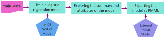
Let's assume that you want to train a logistic regression model on the data in a relation named 'patients' in order to predict the second attack of patients given their treatment and trait anxiety.

After training, the model is shown in a system table named V_CATALOG.MODELS which lists the archived ML models in Vertica.

=> -- Training a logistic regression model on a training_data
=> SELECT logistic_reg('myModel', 'patients', 'second_attack', 'treatment, trait_anxiety');
       logistic_reg
---------------------------
 Finished in 5 iterations

(1 row)

=> -- Looking at the models table
=> SELECT model_name, schema_name, category, model_type, create_time, size FROM models;
 model_name | schema_name |    category    |     model_type      |          create_time          | size
------------+-------------+----------------+---------------------+-------------------------------+------
 myModel    | public      | VERTICA_MODELS | LOGISTIC_REGRESSION | 2020-07-28 00:05:18.441958-04 | 1845
(1 row)

You can look at the summary of the model using the GET_MODEL_SUMMARY function.

=> -- Looking at the summary of the model
=> \t
Showing only tuples.
=> SELECT get_model_summary(USING PARAMETERS model_name='myModel');


=======
details
=======
  predictor  |coefficient|std_err |z_value |p_value
-------------+-----------+--------+--------+--------
  Intercept  | -6.36347  | 3.21390|-1.97998| 0.04771
  treatment  | -1.02411  | 1.17108|-0.87450| 0.38185
trait_anxiety|  0.11904  | 0.05498| 2.16527| 0.03037


==============
regularization
==============
type| lambda
----+--------
none| 1.00000


===========
call_string
===========
logistic_reg('public.myModel', 'patients', '"second_attack"', 'treatment, trait_anxiety'
USING PARAMETERS optimizer='newton', epsilon=1e-06, max_iterations=100, regularization='none', lambda=1, alpha=0.5)

===============
Additional Info
===============
       Name       |Value
------------------+-----
 iteration_count  |  5
rejected_row_count|  0
accepted_row_count| 20

You can also retrieve the model's attributes using the GET_MODEL_ATTRIBUTE function.

=> \t
Tuples only is off.
=> -- The list of the attributes of the model
=> SELECT get_model_attribute(USING PARAMETERS model_name='myModel');
     attr_name      |                    attr_fields                    | #_of_rows
--------------------+---------------------------------------------------+-----------
 details            | predictor, coefficient, std_err, z_value, p_value |         3
 regularization     | type, lambda                                      |         1
 iteration_count    | iteration_count                                   |         1
 rejected_row_count | rejected_row_count                                |         1
 accepted_row_count | accepted_row_count                                |         1
 call_string        | call_string                                       |         1
(6 rows)

=> -- Returning the coefficients of the model in a tabular format
=> SELECT get_model_attribute(USING PARAMETERS model_name='myModel', attr_name='details');
   predictor   |    coefficient    |      std_err       |      z_value       |      p_value
---------------+-------------------+--------------------+--------------------+--------------------
 Intercept     | -6.36346994178182 |   3.21390452471434 |  -1.97998101463435 | 0.0477056620380991
 treatment     | -1.02410605239327 |    1.1710801464903 | -0.874496980810833 |  0.381847663704613
 trait_anxiety | 0.119044916668605 | 0.0549791755747139 |   2.16527285875412 | 0.0303667955962211
(3 rows)

You can use the EXPORT_MODELS function in a simple statement to export the model in PMML format, as shown below.

=> -- Exporting the model as PMML
=> SELECT export_models('/data/username/temp', 'myModel' USING PARAMETERS category='PMML');
 export_models
---------------
 Success
(1 row)

See also

• MODELS
• V_CATALOG schema

8.2.2 - Importing and predicting with PMML models

As a Vertica user, you can train ML models in other platforms, convert them to standard PMML format, and then import them into Vertica for in-database prediction on data stored in Vertica relations.

Here is an example of how to import a PMML model trained in Spark. The following diagram shows the workflow of the example.

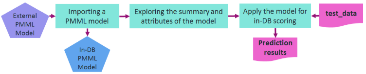
You can use the IMPORT_MODELS function in a simple statement to import the PMML model. The imported model then appears in a system table named V_CATALOG.MODELS which lists the archived ML models in Vertica.

=> -- importing the PMML model trained and generated in Spark
=> SELECT import_models('/data/username/temp/spark_logistic_reg' USING PARAMETERS category='PMML');
 import_models
---------------
 Success
(1 row)

=> -- Looking at the models table=> SELECT model_name, schema_name, category, model_type, create_time, size FROM models;
     model_name     | schema_name | category |      model_type       |          create_time          | size
--------------------+-------------+----------+-----------------------+-------------------------------+------
 spark_logistic_reg | public      | PMML     | PMML_REGRESSION_MODEL | 2020-07-28 00:12:29.389709-04 | 5831
(1 row)

You can look at the summary of the model using GET_MODEL_SUMMARY function.

=> \t
Showing only tuples.
=> SELECT get_model_summary(USING PARAMETERS model_name='spark_logistic_reg');

=============
function_name
=============
classification

===========
data_fields
===========
 name  |dataType|  optype
-------+--------+-----------
field_0| double |continuous
field_1| double |continuous
field_2| double |continuous
field_3| double |continuous
field_4| double |continuous
field_5| double |continuous
field_6| double |continuous
field_7| double |continuous
field_8| double |continuous
target | string |categorical


==========
predictors
==========
 name  |exponent|coefficient
-------+--------+-----------
field_0|   1    | -0.23318
field_1|   1    |  0.73623
field_2|   1    |  0.29964
field_3|   1    |  0.12809
field_4|   1    | -0.66857
field_5|   1    |  0.51675
field_6|   1    | -0.41026
field_7|   1    |  0.30829
field_8|   1    | -0.17788


===============
Additional Info
===============
    Name     | Value
-------------+--------
is_supervised|   1
  intercept  |-1.20173

You can also retrieve the model's attributes using the GET_MODEL_ATTRIBUTE function.

=> \t
Tuples only is off.
=> -- The list of the attributes of the PMML model
=> SELECT get_model_attribute(USING PARAMETERS model_name='spark_logistic_reg');
   attr_name   |         attr_fields         | #_of_rows
---------------+-----------------------------+-----------
 is_supervised | is_supervised               |         1
 function_name | function_name               |         1
 data_fields   | name, dataType, optype      |        10
 intercept     | intercept                   |         1
 predictors    | name, exponent, coefficient |         9
(5 rows)

=> -- The coefficients of the PMML model
=> SELECT get_model_attribute(USING PARAMETERS model_name='spark_logistic_reg', attr_name='predictors');
  name   | exponent |    coefficient
---------+----------+--------------------
 field_0 |        1 |   -0.2331769167607
 field_1 |        1 |  0.736227459496199
 field_2 |        1 |   0.29963728232024
 field_3 |        1 |  0.128085369856188
 field_4 |        1 | -0.668573096260048
 field_5 |        1 |  0.516750679584637
 field_6 |        1 |  -0.41025989394959
 field_7 |        1 |  0.308289533913736
 field_8 |        1 | -0.177878773139411
(9 rows)

You can then use the PREDICT_PMML function to apply the imported model on a relation for in-database prediction. The internal parameters of the model can be matched to the column names of the input relation by their names or their listed position. Direct input values can also be fed to the function as displayed below.

=> -- Using the imported PMML model for scoring direct input values
=> SELECT predict_pmml(1.5,0.5,2,1,0.75,4.2,3.1,0.9,1.1
username(>                     USING PARAMETERS model_name='spark_logistic_reg', match_by_pos=true);
 predict_pmml
--------------
 1
(1 row)

=> -- Using the imported PMML model for scoring samples in a table
=> SELECT predict_pmml(* USING PARAMETERS model_name='spark_logistic_reg') AS prediction
=>     FROM test_data;
 prediction
------------
 1
 0
(2 rows)

See also

• MODELS
• V_CATALOG schema

8.2.3 - PMML features and attributes

To be compatible with Vertica, PMML models must conform to the following:

• The PMML model does not have a data preprocessing step.

• The encoded PMML model type is ClusteringModel, GeneralRegressionModel, MiningModel, RegressionModel, or TreeModel.

Supported PMML tags and attributes

The following table lists supported PMML tags and attributes.