This is the multi-page printable view of this section.
Click here to print.
Return to the regular view of this page.
Time series analytics
Time series analytics evaluate the values of a given set of variables over time and group those values into a window (based on a time interval) for analysis and aggregation.
Time series analytics evaluate the values of a given set of variables over time and group those values into a window (based on a time interval) for analysis and aggregation. Common scenarios for using time series analytics include: stock market trades and portfolio performance changes over time, and charting trend lines over data.
Since both time and the state of data within a time series are continuous, it can be challenging to evaluate SQL queries over time. Input records often occur at non-uniform intervals, which can create gaps. To solve this problem Vertica provides:
-
Gap-filling functionality, which fills in missing data points
-
Interpolation scheme, which constructs new data points within the range of a discrete set of known data points.
Vertica interpolates the non-time series columns in the data (such as analytic function results computed over time slices) and adds the missing data points to the output. This section describes gap filling and interpolation in detail.
You can use event-based windows to break time series data into windows that border on significant events within the data. This is especially relevant in financial data, where analysis might focus on specific events as triggers to other activity.
Sessionization is a special case of event-based windows that is frequently used to analyze click streams, such as identifying web browsing sessions from recorded web clicks.
Vertica provides additional support for time series analytics with the following SQL extensions:
-
TIMESERIES clause in a SELECT statement supports gap-filling and interpolation (GFI) computation.
-
TS_FIRST_VALUE and TS_LAST_VALUE are time series aggregate functions that return the value at the start or end of a time slice, respectively, which is determined by the interpolation scheme.
-
TIME_SLICE is a (SQL extension) date/time function that aggregates data by different fixed-time intervals and returns a rounded-up input TIMESTAMP value to a value that corresponds with the start or end of the time slice interval.
See also
1 - Gap filling and interpolation (GFI)
The examples and graphics that explain the concepts in this topic use the following simple schema:.
The examples and graphics that explain the concepts in this topic use the following simple schema:
CREATE TABLE TickStore (ts TIMESTAMP, symbol VARCHAR(8), bid FLOAT);
INSERT INTO TickStore VALUES ('2009-01-01 03:00:00', 'XYZ', 10.0);
INSERT INTO TickStore VALUES ('2009-01-01 03:00:05', 'XYZ', 10.5);
COMMIT;
In Vertica, time series data is represented by a sequence of rows that conforms to a particular table schema, where one of the columns stores the time information.
Both time and the state of data within a time series are continuous. Thus, evaluating SQL queries over time can be challenging because input records usually occur at non-uniform intervals and can contain gaps.
For example, the following table contains two input rows five seconds apart: 3:00:00 and 3:00:05.
=> SELECT * FROM TickStore;
         ts          | symbol | bid
---------------------+--------+------
 2009-01-01 03:00:00 | XYZ    |   10
 2009-01-01 03:00:05 | XYZ    | 10.5
(2 rows)
Given those two inputs, how can you determine a bid price that falls between the two points, such as at 3:00:03 PM?
The
TIME_SLICE function normalizes timestamps into corresponding time slices; however, TIME_SLICE does not solve the problem of missing inputs (time slices) in the data. Instead, Vertica provides gap-filling and interpolation (GFI) functionality, which fills in missing data points and adds new (missing) data points within a range of known data points to the output. It accomplishes these tasks with the time series aggregate functions (TS_FIRST_VALUE and TS_LAST_VALUE) and the SQL TIMESERIES clause.
But first, we'll illustrate the components that make up gap filling and interpolation in Vertica, starting with Constant interpolation.
The images in the following topics use the following legend:
-
The x-axis represents the timestamp (ts) column
-
The y-axis represents the bid column.
-
The vertical blue lines delimit the time slices.
-
The red dots represent the input records in the table, $10.0 and $10.5.
-
The blue stars represent the output values, including interpolated values.
1.1 - Constant interpolation
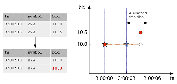
Given known input timestamps at 03:00:00 and 03:00:05 in the sample TickStore schema, how might you determine the bid price at 03:00:03?.
Given known input timestamps at 03:00:00 and 03:00:05 in the sample TickStore schema, how might you determine the bid price at 03:00:03?
A common interpolation scheme used on financial data is to set the bid price to the last seen value so far. This scheme is referred to as constant interpolation, in which Vertica computes a new value based on the previous input records.
Note
Constant is Vertica's default interpolation scheme. Another interpolation scheme,
linear, is discussed in an upcoming topic.
Returning to the problem query, here is the table output, which shows a 5-second lag between bids at 03:00:00 and 03:00:05:
=> SELECT * FROM TickStore;
         ts          | symbol | bid
---------------------+--------+------
 2009-01-01 03:00:00 | XYZ    |   10
 2009-01-01 03:00:05 | XYZ    | 10.5
(2 rows)
Using constant interpolation, the interpolated bid price of XYZ remains at $10.0 at 3:00:03, which falls between the two known data inputs (3:00:00 PM and 3:00:05). At 3:00:05, the value changes to $10.5. The known data points are represented by a red dot, and the interpolated value at 3:00:03 is represented by the blue star.
In order to write a query that makes the input rows more uniform, you first need to understand the TIMESERIES clause and time series aggregate functions.
1.2 - TIMESERIES clause and aggregates
The SELECT..TIMESERIES clause and time series aggregates help solve the problem of gaps in input records by normalizing the data into 3-second time slices and interpolating the bid price when it finds gaps.
The SELECT..TIMESERIES clause and time series aggregates help solve the problem of gaps in input records by normalizing the data into 3-second time slices and interpolating the bid price when it finds gaps.
TIMESERIES clause
The TIMESERIES clause is an important component of time series analytics computation. It performs gap filling and interpolation (GFI) to generate time slices missing from the input records. The clause applies to the timestamp columns/expressions in the data, and takes the following form:
TIMESERIES slice_time AS 'length_and_time_unit_expression'
OVER ( ... [ window-partition-clause[ , ... ] ]
... ORDER BY time_expression )
... [ ORDER BY table_column [ , ... ] ]
Note
The TIMESERIES clause requires an ORDER BY operation on the timestamp column.
Time series aggregate functions
The Timeseries Aggregate (TSA) functions TS_FIRST_VALUE and TS_LAST_VALUE evaluate the values of a given set of variables over time and group those values into a window for analysis and aggregation.
TSA functions process the data that belongs to each time slice. One output row is produced per time slice or per partition per time slice if a partition expression is present.
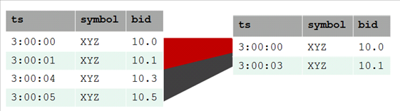
The following table shows 3-second time slices where:
-
The first two rows fall within the first time slice, which runs from 3:00:00 to 3:00:02. These are the input rows for the TSA function's output for the time slice starting at 3:00:00.
-
The second two rows fall within the second time slice, which runs from 3:00:03 to 3:00:05. These are the input rows for the TSA function's output for the time slice starting at 3:00:03.
The result is the start of each time slice.
Examples
The following examples compare the values returned with and without the TS_FIRST_VALUE TSA function.
This example shows the TIMESERIES clause without the TS_FIRST_VALUE TSA function.
=> SELECT slice_time, bid FROM TickStore TIMESERIES slice_time AS '3 seconds' OVER(PARTITION by TickStore.bid ORDER BY ts);
This example shows both the TIMESERIES clause and the TS_FIRST_VALUE TSA function. The query returns the values of the bid column, as determined by the specified constant interpolation scheme.
=> SELECT slice_time, TS_FIRST_VALUE(bid, 'CONST') bid FROM TickStore
   TIMESERIES slice_time AS '3 seconds' OVER(PARTITION by symbol ORDER BY ts);
Vertica interpolates the last known value and fills in the missing datapoint, returning 10 at 3:00:03:
|
First query |
|
Interpolated value |
     slice_time      | bid
---------------------+-----
 2009-01-01 03:00:00 |  10
 2009-01-01 03:00:03 | 10.5
(2 rows)
|
==> |
     slice_time      | bid
---------------------+-----
 2009-01-01 03:00:00 |  10
 2009-01-01 03:00:03 |  10
(2 rows)
|
1.3 - Time series rounding
Vertica calculates all time series as equal intervals relative to the timestamp 2000-01-01 00:00:00.
Vertica calculates all time series as equal intervals relative to the timestamp 2000-01-01 00:00:00. Vertica rounds time series timestamps as needed, to conform with this baseline. Start times are also rounded down to the nearest whole unit for the specified interval.
Given this logic, the TIMESERIES clause generates series of timestamps as described in the following sections.
Minutes
Time series of minutes are rounded down to full minutes. For example, the following statement specifies a time span of 00:00:03 ‑ 00:05:50:
=> SELECT ts FROM (
    SELECT '2015-01-04 00:00:03'::TIMESTAMP AS tm
      UNION
    SELECT '2015-01-04 00:05:50'::TIMESTAMP AS tm
   ) t
   TIMESERIES ts AS '1 minute' OVER (ORDER BY tm);
Vertica rounds down the time series start and end times to full minutes, 00:00:00 and 00:05:00, respectively:
         ts
---------------------
 2015-01-04 00:00:00
 2015-01-04 00:01:00
 2015-01-04 00:02:00
 2015-01-04 00:03:00
 2015-01-04 00:04:00
 2015-01-04 00:05:00
(6 rows)
Weeks
Because the baseline timestamp 2000-01-01 00:00:00 is a Saturday, all time series of weeks start on Saturday. Vertica rounds down the series start and end timestamps accordingly. For example, the following statement specifies a time span of 12/10/99 ‑ 01/10/00:
=> SELECT ts FROM (
     SELECT '1999-12-10 00:00:00'::TIMESTAMP AS tm
       UNION
     SELECT '2000-01-10 23:59:59'::TIMESTAMP AS tm
     ) t
     TIMESERIES ts AS '1 week' OVER (ORDER BY tm);
The specified time span starts on Friday (12/10/99), so Vertica starts the time series on the preceding Saturday, 12/04/99. The time series ends on the last Saturday within the time span, 01/08/00:
         ts
---------------------
 1999-12-04 00:00:00
 1999-12-11 00:00:00
 1999-12-18 00:00:00
 1999-12-25 00:00:00
 2000-01-01 00:00:00
 2000-01-08 00:00:00
(6 rows)
Months
Time series of months are divided into equal 30-day intervals, relative to the baseline timestamp 2000-01-01 00:00:00. For example, the following statement specifies a time span of 09/01/99 ‑ 12/31/00:
=> SELECT ts FROM (
     SELECT '1999-09-01 00:00:00'::TIMESTAMP AS tm
       UNION
     SELECT '2000-12-31 23:59:59'::TIMESTAMP AS tm
   ) t
   TIMESERIES ts AS '1 month' OVER (ORDER BY tm);
Vertica generates a series of 30-day intervals, where each timestamp is rounded up or down, relative to the baseline timestamp:
         ts
---------------------
 1999-08-04 00:00:00
 1999-09-03 00:00:00
 1999-10-03 00:00:00
 1999-11-02 00:00:00
 1999-12-02 00:00:00
 2000-01-01 00:00:00
 2000-01-31 00:00:00
 2000-03-01 00:00:00
 2000-03-31 00:00:00
 2000-04-30 00:00:00
 2000-05-30 00:00:00
 2000-06-29 00:00:00
 2000-07-29 00:00:00
 2000-08-28 00:00:00
 2000-09-27 00:00:00
 2000-10-27 00:00:00
 2000-11-26 00:00:00
 2000-12-26 00:00:00
(18 rows)
Years
Time series of years are divided into equal 365-day intervals. If a time span overlaps leap years since or before the baseline timestamp 2000-01-01 00:00:00, Vertica rounds the series timestamps accordingly.
For example, the following statement specifies a time span of 01/01/95 ‑ 05/08/09, which overlaps four leap years, including the baseline timestamp:
=> SELECT ts FROM (
      SELECT '1995-01-01 00:00:00'::TIMESTAMP AS tm
        UNION
      SELECT '2009-05-08'::TIMESTAMP AS tm
    ) t timeseries ts AS '1 year' over (ORDER BY tm);
Vertica generates a series of timestamps that are rounded up or down, relative to the baseline timestamp:
         ts
---------------------
 1994-01-02 00:00:00
 1995-01-02 00:00:00
 1996-01-02 00:00:00
 1997-01-01 00:00:00
 1998-01-01 00:00:00
 1999-01-01 00:00:00
 2000-01-01 00:00:00
 2000-12-31 00:00:00
 2001-12-31 00:00:00
 2002-12-31 00:00:00
 2003-12-31 00:00:00
 2004-12-30 00:00:00
 2005-12-30 00:00:00
 2006-12-30 00:00:00
 2007-12-30 00:00:00
 2008-12-29 00:00:00
(16 rows)
1.4 - Linear interpolation
Instead of interpolating data points based on the last seen value (constant interpolation), linear interpolation is where Vertica interpolates values in a linear slope based on the specified time slice.
Instead of interpolating data points based on the last seen value (Constant interpolation), linear interpolation is where Vertica interpolates values in a linear slope based on the specified time slice.
The query that follows uses linear interpolation to place the input records in 2-second time slices and return the first bid value for each symbol/time slice combination (the value at the start of the time slice):
=> SELECT slice_time, TS_FIRST_VALUE(bid, 'LINEAR') bid FROM Tickstore
   TIMESERIES slice_time AS '2 seconds' OVER(PARTITION BY symbol ORDER BY ts);
     slice_time      | bid
---------------------+------
 2009-01-01 03:00:00 |   10
 2009-01-01 03:00:02 | 10.2
 2009-01-01 03:00:04 | 10.4
(3 rows)
The following figure illustrates the previous query results, showing the 2-second time gaps (3:00:02 and 3:00:04) in which no input record occurs. Note that the interpolated bid price of XYZ changes to 10.2 at 3:00:02 and 10.3 at 3:00:03 and 10.4 at 3:00:04, all of which fall between the two known data inputs (3:00:00 and 3:00:05). At 3:00:05, the value would change to 10.5.
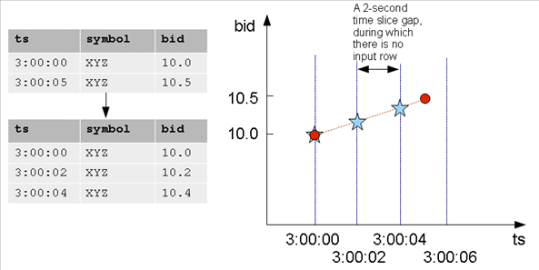
Note
The known data points above are represented by a red dot, and the interpolated values are represented by blue stars.
The following is a side-by-side comparison of constant and linear interpolation schemes.
|
CONST interpolation |
LINEAR interpolation |
 |
 |
1.5 - GFI examples
This topic illustrates some of the queries you can write using the constant and linear interpolation schemes.
This topic illustrates some of the queries you can write using the constant and linear interpolation schemes.
Constant interpolation
The first query uses TS_FIRST_VALUE() and the TIMESERIES clause to place the input records in 3-second time slices and return the first bid value for each symbol/time slice combination (the value at the start of the time slice).
Note
The TIMESERIES clause requires an ORDER BY operation on the TIMESTAMP column.
=> SELECT slice_time, symbol, TS_FIRST_VALUE(bid) AS first_bid FROM TickStore
   TIMESERIES slice_time AS '3 seconds' OVER (PARTITION BY symbol ORDER BY ts);
Because the bid price of stock XYZ is 10.0 at 3:00:03, the first_bid value of the second time slice, which starts at 3:00:03 is till 10.0 (instead of 10.5) because the input value of 10.5 does not occur until 3:00:05. In this case, the interpolated value is inferred from the last value seen on stock XYZ for time 3:00:03:
     slice_time      | symbol | first_bid
---------------------+--------+-----------
 2009-01-01 03:00:00 | XYZ    |        10
 2009-01-01 03:00:03 | XYZ    |        10
(2 rows)
The next example places the input records in 2-second time slices to return the first bid value for each symbol/time slice combination:
=> SELECT slice_time, symbol, TS_FIRST_VALUE(bid) AS first_bid FROM TickStore
   TIMESERIES slice_time AS '2 seconds' OVER (PARTITION BY symbol ORDER BY ts);
The result now contains three records in 2-second increments, all of which occur between the first input row at 03:00:00 and the second input row at 3:00:05. Note that the second and third output record correspond to a time slice where there is no input record:
     slice_time      | symbol | first_bid
---------------------+--------+-----------
 2009-01-01 03:00:00 | XYZ    |        10
2009-01-01 03:00:02 | XYZ    |        10
2009-01-01 03:00:04 | XYZ    |        10
(3 rows)
Using the same table schema, the next query uses TS_LAST_VALUE(), with the TIMESERIES clause to return the last values of each time slice (the values at the end of the time slices).
Note
Time series aggregate functions process the data that belongs to each time slice. One output row is produced per time slice or per partition per time slice if a partition expression is present.
=> SELECT slice_time, symbol, TS_LAST_VALUE(bid) AS last_bid FROM TickStore
   TIMESERIES slice_time AS '2 seconds' OVER (PARTITION BY symbol ORDER BY ts);
Notice that the last value output row is 10.5 because the value 10.5 at time 3:00:05 was the last point inside the 2-second time slice that started at 3:00:04:
     slice_time      | symbol | last_bid
---------------------+--------+----------
 2009-01-01 03:00:00 | XYZ    |       10
 2009-01-01 03:00:02 | XYZ    |       10
 2009-01-01 03:00:04 | XYZ    |     10.5
(3 rows)
Remember that because constant interpolation is the default, the same results are returned if you write the query using the CONST parameter as follows:
=> SELECT slice_time, symbol, TS_LAST_VALUE(bid, 'CONST') AS last_bid FROM TickStore
   TIMESERIES slice_time AS '2 seconds' OVER (PARTITION BY symbol ORDER BY ts);
Linear interpolation
Based on the same input records described in the constant interpolation examples, which specify 2-second time slices, the result of TS_LAST_VALUE with linear interpolation is as follows:
=> SELECT slice_time, symbol, TS_LAST_VALUE(bid, 'linear') AS last_bid   FROM TickStore
   TIMESERIES slice_time AS '2 seconds' OVER (PARTITION BY symbol ORDER BY ts);
In the results, no last_bid value is returned for the last row because the query specified TS_LAST_VALUE, and there is no data point after the 3:00:04 time slice to interpolate.
     slice_time      | symbol | last_bid
---------------------+--------+----------
 2009-01-01 03:00:00 | XYZ    |     10.2
 2009-01-01 03:00:02 | XYZ    |     10.4
 2009-01-01 03:00:04 | XYZ    |
(3 rows)
Using multiple time series aggregate functions
Multiple time series aggregate functions can exists in the same query. They share the same gap-filling policy as defined in the TIMESERIES clause; however, each time series aggregate function can specify its own interpolation policy. In the following example, there are two constant and one linear interpolation schemes, but all three functions use a three-second time slice:
=> SELECT slice_time, symbol,
       TS_FIRST_VALUE(bid, 'const') fv_c,
       TS_FIRST_VALUE(bid, 'linear') fv_l,
       TS_LAST_VALUE(bid, 'const') lv_c
   FROM TickStore
   TIMESERIES slice_time AS '3 seconds' OVER(PARTITION BY symbol ORDER BY ts);
In the following output, the original output is compared to output returned by multiple time series aggregate functions.
    ts    | symbol | bid
----------+--------+------
 03:00:00 | XYZ    |   10
 03:00:05 | XYZ    | 10.5
(2 rows)
|
==> |
     slice_time      | symbol | fv_c | fv_l | lv_c
---------------------+--------+------+------+------
 2009-01-01 03:00:00 | XYZ    |   10 |   10 |   10
 2009-01-01 03:00:03 | XYZ    |   10 | 10.3 | 10.5
(2 rows)
|
Using the analytic LAST_VALUE function
Here's an example using LAST_VALUE(), so you can see the difference between it and the GFI syntax.
=> SELECT *, LAST_VALUE(bid) OVER(PARTITION by symbol ORDER BY ts)
   AS "last bid" FROM TickStore;
There is no gap filling and interpolation to the output values.
         ts          | symbol | bid  | last bid
---------------------+--------+------+----------
 2009-01-01 03:00:00 | XYZ    |   10 |       10
 2009-01-01 03:00:05 | XYZ    | 10.5 |     10.5
(2 rows)
Using slice_time
In a TIMESERIES query, you cannot use the column slice_time in the WHERE clause because the WHERE clause is evaluated before the TIMESERIES clause, and the slice_time column is not generated until the TIMESERIES clause is evaluated. For example, Vertica does not support the following query:
=> SELECT symbol, slice_time, TS_FIRST_VALUE(bid IGNORE NULLS) AS fv
   FROM TickStore
   WHERE slice_time = '2009-01-01 03:00:00'
   TIMESERIES slice_time as '2 seconds' OVER (PARTITION BY symbol ORDER BY ts);
ERROR:  Time Series timestamp alias/Time Series Aggregate Functions not allowed in WHERE clause
Instead, you could write a subquery and put the predicate on slice_time in the outer query:
=> SELECT * FROM (
      SELECT symbol, slice_time,
        TS_FIRST_VALUE(bid IGNORE NULLS) AS fv
      FROM TickStore
      TIMESERIES slice_time AS '2 seconds'
      OVER (PARTITION BY symbol ORDER BY ts) ) sq
   WHERE slice_time = '2009-01-01 03:00:00';
 symbol |     slice_time      | fv
--------+---------------------+----
 XYZ    | 2009-01-01 03:00:00 | 10
(1 row)
Creating a dense time series
The TIMESERIES clause provides a convenient way to create a dense time series for use in an outer join with fact data. The results represent every time point, rather than just the time points for which data exists.
The examples that follow use the same TickStore schema described in Gap filling and interpolation (GFI), along with the addition of a new inner table for the purpose of creating a join:
=> CREATE TABLE inner_table (
       ts TIMESTAMP,
       bid FLOAT
   );
=> CREATE PROJECTION inner_p (ts, bid) as SELECT * FROM inner_table
   ORDER BY ts, bid UNSEGMENTED ALL NODES;
=> INSERT INTO inner_table VALUES ('2009-01-01 03:00:02', 1);
=> INSERT INTO inner_table VALUES ('2009-01-01 03:00:04', 2);
=> COMMIT;
You can create a simple union between the start and end range of the timeframe of interest in order to return every time point. This example uses a 1-second time slice:
=> SELECT ts FROM (
     SELECT '2009-01-01 03:00:00'::TIMESTAMP AS time FROM TickStore
     UNION
     SELECT '2009-01-01 03:00:05'::TIMESTAMP FROM TickStore) t
   TIMESERIES ts AS '1 seconds' OVER(ORDER BY time);
         ts
---------------------
 2009-01-01 03:00:00
 2009-01-01 03:00:01
 2009-01-01 03:00:02
 2009-01-01 03:00:03
 2009-01-01 03:00:04
 2009-01-01 03:00:05
(6 rows)
The next query creates a union between the start and end range of the timeframe using 500-millisecond time slices:
=> SELECT ts FROM (
     SELECT '2009-01-01 03:00:00'::TIMESTAMP AS time
     FROM TickStore
     UNION
     SELECT '2009-01-01 03:00:05'::TIMESTAMP FROM TickStore) t
   TIMESERIES ts AS '500 milliseconds' OVER(ORDER BY time);
          ts
-----------------------
 2009-01-01 03:00:00
 2009-01-01 03:00:00.5
 2009-01-01 03:00:01
 2009-01-01 03:00:01.5
 2009-01-01 03:00:02
 2009-01-01 03:00:02.5
 2009-01-01 03:00:03
 2009-01-01 03:00:03.5
 2009-01-01 03:00:04
 2009-01-01 03:00:04.5
 2009-01-01 03:00:05
(11 rows)
The following query creates a union between the start- and end-range of the timeframe of interest using 1-second time slices:
=> SELECT * FROM (
     SELECT ts FROM (
       SELECT '2009-01-01 03:00:00'::timestamp AS time FROM TickStore
       UNION
       SELECT '2009-01-01 03:00:05'::timestamp FROM TickStore) t
       TIMESERIES ts AS '1 seconds' OVER(ORDER BY time) ) AS outer_table
   LEFT OUTER JOIN inner_table ON outer_table.ts = inner_table.ts;
The union returns a complete set of records from the left-joined table with the matched records in the right-joined table. Where the query found no match, it extends the right side column with null values:
         ts          |         ts          | bid
---------------------+---------------------+-----
 2009-01-01 03:00:00 |                     |
 2009-01-01 03:00:01 |                     |
 2009-01-01 03:00:02 | 2009-01-01 03:00:02 |   1
 2009-01-01 03:00:03 |                     |
 2009-01-01 03:00:04 | 2009-01-01 03:00:04 |   2
 2009-01-01 03:00:05 |                     |
(6 rows)
2 - Null values in time series data
Null values are uncommon inputs for gap-filling and interpolation (GFI) computation.
Null values are uncommon inputs for gap-filling and interpolation (GFI) computation. When null values exist, you can use time series aggregate (TSA) functions
TS_FIRST_VALUE and
TS_LAST_VALUE with IGNORE NULLS to affect output of the interpolated values. TSA functions are treated like their analytic counterparts
FIRST_VALUE and
LAST_VALUE: if the timestamp itself is null, Vertica filters out those rows before gap filling and interpolation occurs.
Constant interpolation with null values
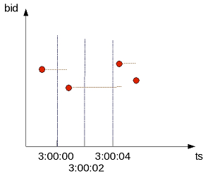
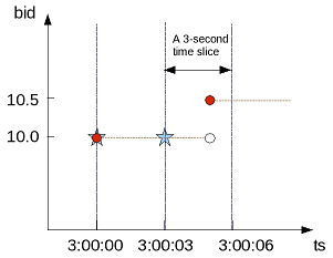
Figure 1 illustrates a default (constant) interpolation result on four input rows where none of the inputs contains a NULL value:
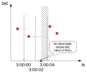
Figure 2 shows the same input rows with the addition of another input record whose bid value is NULL, and whose timestamp (ts) value is 3:00:03:
For constant interpolation, the bid value starting at 3:00:03 is null until the next non-null bid value appears in time. In Figure 2, the presence of the null row makes the interpolated bid value null in the time interval denoted by the shaded region. If TS_FIRST_VALUE(bid) is evaluated with constant interpolation on the time slice that begins at 3:00:02, its output is non-null. However, TS_FIRST_VALUE(bid) on the next time slice produces null. If the last value of the 3:00:02 time slice is null, the first value for the next time slice (3:00:04) is null. However, if you use a TSA function with IGNORE NULLS, then the value at 3:00:04 is the same value as it was at 3:00:02.
To illustrate, insert a new row into the TickStore table at 03:00:03 with a null bid value, Vertica outputs a row for the 03:00:02 record with a null value but no row for the 03:00:03 input:
=> INSERT INTO tickstore VALUES('2009-01-01 03:00:03', 'XYZ', NULL);
=> SELECT slice_time, symbol, TS_LAST_VALUE(bid) AS last_bid FROM TickStore
-> TIMESERIES slice_time AS '2 seconds' OVER (PARTITION BY symbol ORDER BY ts);
     slice_time      | symbol | last_bid
---------------------+--------+----------
 2009-01-01 03:00:00 | XYZ    |       10
 2009-01-01 03:00:02 | XYZ    |
 2009-01-01 03:00:04 | XYZ    |     10.5
(3 rows)
If you specify IGNORE NULLS, Vertica fills in the missing data point using a constant interpolation scheme. Here, the bid price at 03:00:02 is interpolated to the last known input record for bid, which was $10 at 03:00:00:
=> SELECT slice_time, symbol, TS_LAST_VALUE(bid IGNORE NULLS) AS last_bid FROM TickStore
     TIMESERIES slice_time AS '2 seconds' OVER (PARTITION BY symbol ORDER BY ts);
     slice_time      | symbol | last_bid
---------------------+--------+----------
 2009-01-01 03:00:00 | XYZ    |       10
 2009-01-01 03:00:02 | XYZ    |       10
 2009-01-01 03:00:04 | XYZ    |     10.5
(3 rows)
Now, if you insert a row where the timestamp column contains a null value, Vertica filters out that row before gap filling and interpolation occurred.
=> INSERT INTO tickstore VALUES(NULL, 'XYZ', 11.2);
=> SELECT slice_time, symbol, TS_LAST_VALUE(bid) AS last_bid FROM TickStore
     TIMESERIES slice_time AS '2 seconds' OVER (PARTITION BY symbol ORDER BY ts);
Notice there is no output for the 11.2 bid row:
     slice_time      | symbol | last_bid
---------------------+--------+----------
 2009-01-01 03:00:00 | XYZ    |       10
 2009-01-01 03:00:02 | XYZ    |
 2009-01-01 03:00:04 | XYZ    |     10.5
(3 rows)
Linear interpolation with null values
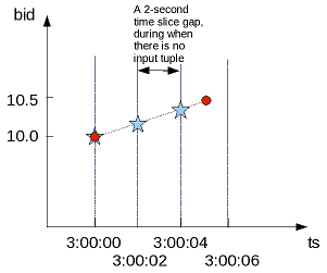
For linear interpolation, the interpolated bid value becomes null in the time interval, represented by the shaded region in Figure 3:
In the presence of an input null value at 3:00:03, Vertica cannot linearly interpolate the bid value around that time point.
Vertica takes the closest non null value on either side of the time slice and uses that value. For example, if you use a linear interpolation scheme and do not specify IGNORE NULLS, and your data has one real value and one null, the result is null. If the value on either side is null, the result is null. Therefore, to evaluate TS_FIRST_VALUE(bid) with linear interpolation on the time slice that begins at 3:00:02, its output is null. TS_FIRST_VALUE(bid) on the next time slice remains null.
=> SELECT slice_time, symbol, TS_FIRST_VALUE(bid, 'linear') AS fv_l FROM TickStore
     TIMESERIES slice_time AS '2 seconds' OVER (PARTITION BY symbol ORDER BY ts);
     slice_time      | symbol | fv_l
---------------------+--------+------
 2009-01-01 03:00:00 | XYZ    |   10
 2009-01-01 03:00:02 | XYZ    |
 2009-01-01 03:00:04 | XYZ    |
(3 rows)