This section covers the following topics:
-
Query plans: Describes how Vertica creates and uses query plans, which optimize access to information in the Vertica database.
-
Directed queries: Shows how to save query plan information.
This is the multi-page printable view of this section. Click here to print.
This section covers the following topics:
Query plans: Describes how Vertica creates and uses query plans, which optimize access to information in the Vertica database.
Directed queries: Shows how to save query plan information.
When you submit a query, the query optimizer quickly chooses the projections to use, optimizes and plans the query execution, and logs the SQL statement to its log. This planning results in an query plan, which maps out the steps the query performs.
A query plan is a sequence of step-like paths that the Vertica cost-based query optimizer uses to execute queries. Vertica can produce different query plans for a given query. For each query plan, the query optimizer evaluates the data to be queried: number of rows, column statistics such as number of distinct values (cardinality), distribution of data across nodes. It also evaluates available resources such as CPUs and network topology, and other environment factors. The query optimizer uses this information to develop several potential plans. It then compares plans and chooses one, generally the plan with the lowest cost.
The optimizer breaks down the query plan into smaller local plans and distributes them to executor nodes. The executor nodes process the smaller plans in parallel. Tasks associated with a query are recorded in the executor's log files.
In the final stages of query plan execution, the initiator node performs the following tasks:
Combines results in a grouping operation.
Merges multiple sorted partial result sets from all the executors.
Formats the results to return to the client.
Before executing a query, you can view its plan in by embedding the query in an EXPLAIN statement; you can also view it in the Management Console.
You can obtain query plans in two ways:
You can also observe the real-time flow of data through a query plan by querying the system table QUERY_PLAN_PROFILES. For more information, see Profiling query plans.
By default, EXPLAIN output represents the query plan as a hierarchy, where each level, or path, represents a single database operation that the optimizer uses to execute a query. EXPLAIN output also appends DOT language source so you can display this output graphically with open source Graphviz tools.
EXPLAIN supports options for producing verbose and JSON output. You can also show the local query plans that are assigned to each node, which together comprise the total (global) query plan.
EXPLAIN also supports an ANNOTATED option. EXPLAIN ANNOTATED returns a query with embedded optimizer hints, which encapsulate the query plan for this query. For an example of usage, see Using optimizer-generated and custom directed queries together.
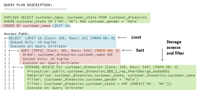
EXPLAIN returns the optimizer's query plan for executing a specified query. For example:
 QUERY PLAN DESCRIPTION:
 ------------------------------

 EXPLAIN SELECT customer_name, customer_state FROM customer_dimension WHERE customer_state IN ('MA','NH') AND customer_gender='Male' ORDER BY customer_name LIMIT 10;

 Access Path:
 +-SELECT  LIMIT 10 [Cost: 365, Rows: 10] (PATH ID: 0)
 |  Output Only: 10 tuples
 |  Execute on: Query Initiator
 | +---> SORT [TOPK] [Cost: 365, Rows: 544] (PATH ID: 1)
 | |      Order: customer_dimension.customer_name ASC
 | |      Output Only: 10 tuples
 | |      Execute on: Query Initiator
 | | +---> STORAGE ACCESS for customer_dimension [Cost: 326, Rows: 544] (PATH ID: 2)
 | | |      Projection: public.customer_dimension_DBD_1_rep_VMartDesign_node0001
 | | |      Materialize: customer_dimension.customer_state, customer_dimension.customer_name
 | | |      Filter: (customer_dimension.customer_gender = 'Male')
 | | |      Filter: (customer_dimension.customer_state = ANY (ARRAY['MA', 'NH']))
 | | |      Execute on: Query Initiator
 | | |      Runtime Filter: (SIP1(TopK): customer_dimension.customer_name)
You can use EXPLAIN to evaluate choices that the optimizer makes with respect to a given query. If you think query performance is less than optimal, run it through the Database Designer. For more information, see Incremental Design and Reducing query run time.
EXPLAIN JSON returns a query plan in JSON format. For example:
=> EXPLAIN JSON SELECT customer_name, customer_state FROM customer_dimension
     WHERE customer_state IN ('MA','NH') AND customer_gender='Male' ORDER BY customer_name LIMIT 10;
 ------------------------------
{
     "PARAMETERS" : {
         "QUERY_STRING" : "EXPLAIN JSON SELECT customer_name, customer_state FROM customer_dimension \n
         WHERE customer_state IN ('MA','NH') AND customer_gender='Male' ORDER BY customer_name LIMIT 10;"
     },
     "PLAN" : {
         "PATH_ID" : 0,
         "PATH_NAME" : "SELECT",
         "EXTRA" : " LIMIT 10",
         "COST" : 2114.000000,
         "ROWS" : 10.000000,
         "COST_STATUS" : "NO_STATISTICS",
         "TUPLE_LIMIT" : 10,
         "EXECUTE_NODE" : "Query Initiator",
         "INPUT" : {
             "PATH_ID" : 1,
             "PATH_NAME" : "SORT",
             "EXTRA" : "[TOPK]",
             "COST" : 2114.000000,
             "ROWS" : 49998.000000,
             "COST_STATUS" : "NO_STATISTICS",
             "ORDER" : ["customer_dimension.customer_name", "customer_dimension.customer_state"],
             "TUPLE_LIMIT" : 10,
             "EXECUTE_NODE" : "All Nodes",
             "INPUT" : {
                 "PATH_ID" : 2,
                 "PATH_NAME" : "STORAGE ACCESS",
                 "EXTRA" : "for customer_dimension",
                 "COST" : 252.000000,
                 "ROWS" : 49998.000000,
                 "COST_STATUS" : "NO_STATISTICS",
                 "TABLE" : "public.customer_dimension",
                 "PROJECTION" : "public.customer_dimension_b0",
                 "MATERIALIZE" : ["customer_dimension.customer_name", "customer_dimension.customer_state"],
                 "FILTER" : ["(customer_dimension.customer_state = ANY (ARRAY['MA', 'NH']))", "(customer_dimension.customer_gender = 'Male')"],
                 "EXECUTE_NODE" : "All Nodes"
          "SIP" : "Runtime Filter: (SIP1(TopK): customer_dimension.customer_name)"

             }
         }
     }
 }
(40 rows)
You can qualify EXPLAIN with the VERBOSE option. This option, valid for default and JSON output, increases the amount of detail in the rendered query plan
For example, the following EXPLAIN statement specifies to produce verbose output. Added information is set off in bold:
=> EXPLAIN VERBOSE SELECT customer_name, customer_state FROM customer_dimension
     WHERE customer_state IN ('MA','NH') AND customer_gender='Male' ORDER BY customer_name LIMIT 10;

QUERY PLAN DESCRIPTION:
 ------------------------------

 Opt Vertica Options
 --------------------
 PLAN_OUTPUT_SUPER_VERBOSE

 EXPLAIN VERBOSE SELECT customer_name, customer_state FROM customer_dimension
 WHERE customer_state IN ('MA','NH') AND customer_gender='Male'
 ORDER BY customer_name LIMIT 10;

Access Path:
+-SELECT  LIMIT 10 [Cost: 756.000000, Rows: 10.000000 Disk(B): 0.000000 CPU(B): 0.000000 Memory(B): 0.000000 Netwrk(B): 0.000000 Parallelism: 1.000000] [OutRowSz (B): 274](PATH ID: 0)
|  Output Only: 10 tuples
|  Execute on: Query Initiator
|  Sort Key: (customer_dimension.customer_name)
|  LDISTRIB_UNSEGMENTED
| +---> SORT [TOPK] [Cost: 756.000000, Rows: 9998.000000 Disk(B): 0.000000 CPU(B): 34274697.123457 Memory(B): 2739452.000000 Netwrk(B): 0.000000 Parallelism: 4.000000 (NO STATISTICS)] [OutRowSz (B): 274] (PATH ID: 1)
| |      Order: customer_dimension.customer_name ASC
| |      Output Only: 10 tuples
| |      Execute on: Query Initiator
| |      Sort Key: (customer_dimension.customer_name)
| |      LDISTRIB_UNSEGMENTED
| | +---> STORAGE ACCESS for customer_dimension [Cost: 513.000000, Rows: 9998.000000 Disk(B): 0.000000 CPU(B): 0.000000 Memory(B): 0.000000 Netwrk(B): 0.000000 Parallelism: 4.000000 (NO STATISTICS)] [OutRowSz (B): 274] (PATH ID: 2)
| | |      Column Cost Aspects: [ Disk(B): 7371817.156569 CPU(B): 4914708.578284 Memory(B): 2659466.004399 Netwrk(B): 0.000000 Parallelism: 4.000000 ]
| | |      Projection: public.customer_dimension_P1
| | |      Materialize: customer_dimension.customer_state, customer_dimension.customer_name
| | |      Filter: (customer_dimension.customer_gender = 'Male')/* sel=0.999800 ndv= 500 */
| | |      Filter: (customer_dimension.customer_state = ANY (ARRAY['MA', 'NH']))/* sel=0.999800 ndv= 500 */
| | |      Execute on: All Nodes
| | |      Runtime Filter: (SIP1(TopK): customer_dimension.customer_name)
| | |      Sort Key: (customer_dimension.household_id, customer_dimension.customer_key, customer_dimension.store_membership_card, customer_dimension.customer_type, customer_dimension.customer_region, customer_dimension.title, customer_dimension.number_of_children)
| | |      LDISTRIB_SEGMENTED
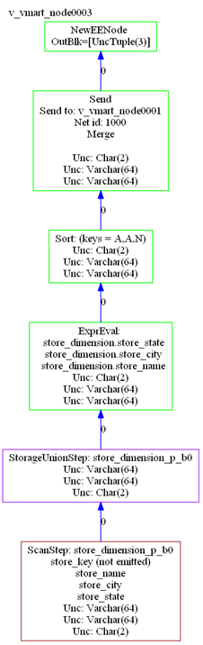
EXPLAIN LOCAL (on a multi-node database) shows the local query plans assigned to each node, which together comprise the total (global) query plan. If you omit this option, Vertica shows only the global query plan. Local query plans are shown only in DOT language source, which can be rendered in Graphviz.
For example, the following EXPLAIN statement includes the LOCAL option:
=> EXPLAIN LOCAL SELECT store_name, store_city, store_state
   FROM store.store_dimension ORDER BY store_state ASC, store_city ASC;
The output includes GraphViz source, which describes the local query plans assigned to each node. For example, output for this statement on a three-node database includes a GraphViz description of the following query plan for one node (v_vmart_node0003):
 -----------------------------------------------
 PLAN: v_vmart_node0003 (GraphViz Format)
 -----------------------------------------------
 digraph G {
 graph [rankdir=BT, label = "v_vmart_node0003\n", labelloc=t, labeljust=l ordering=out]
 0[label = "NewEENode \nOutBlk=[UncTuple(3)]", color = "green", shape = "box"];
 1[label = "Send\nSend to: v_vmart_node0001\nNet id: 1000\nMerge\n\nUnc: Char(2)\nUnc: Varchar(64)\nUnc: Varchar(64)", color = "green", shape = "box"];
 2[label = "Sort: (keys = A,A,N)\nUnc: Char(2)\nUnc: Varchar(64)\nUnc: Varchar(64)", color = "green", shape = "box"];
 3[label = "ExprEval: \n  store_dimension.store_state\n  store_dimension.store_city\n  store_dimension.store_name\nUnc: Char(2)\nUnc: Varchar(64)\nUnc: Varchar(64)
", color = "green", shape = "box"];
 4[label = "StorageUnionStep: store_dimension_p_b0\nUnc: Varchar(64)\nUnc: Varchar(64)\nUnc: Char(2)", color = "purple", shape = "box"];
 5[label = "ScanStep: store_dimension_p_b0\nstore_key (not emitted)\nstore_name\nstore_city\nstore_state\nUnc: Varchar(64)\nUnc: Varchar(64)\nUnc: Char(2)", color
= "brown", shape = "box"];
 1->0 [label = "0",color = "blue"];
 2->1 [label = "0",color = "blue"];
 3->2 [label = "0",color = "blue"];
 4->3 [label = "0",color = "blue"];
 5->4 [label = "0",color = "blue"];
 }
GraphViz renders this output as follows:
The query optimizer chooses a query plan based on cost estimates. The query optimizer uses information from a number of sources to develop potential plans and determine their relative costs. These include:
Number of table rows
Column statistics, including: number of distinct values (cardinality), minimum/maximum values, distribution of values, and disk space usage
Access path that is likely to require fewest I/O operations, and lowest CPU, memory, and network usage
Available eligible projections
Join options: join types (merge versus hash joins), join order
Query predicates
Data segmentation across cluster nodes
Many important optimizer decisions rely on statistics, which the query optimizer uses to determine the final plan to execute a query. Therefore, it is important that statistics be up to date. Without reasonably accurate statistics, the optimizer could choose a suboptimal plan, which might affect query performance.
Vertica provides hints about statistics in the query plan. See Query plan statistics.
Although costs correlate to query runtime, they do not provide an estimate of actual runtime. For example, if the optimizer determines that Plan A costs twice as much as Plan B, it is likely that Plan A will require more time to run. However, this cost estimate does not necessarily indicate that Plan A will run twice as long as Plan B.
Also, plan costs for different queries are not directly comparable. For example, if the estimated cost of Plan X for query1 is greater than the cost of Plan Y for query2, it is not necessarily true that Plan X's runtime is greater than Plan Y's runtime.
Depending on the query and database schema, EXPLAIN output includes the following information:
Tables referenced by the statement
Estimated costs
Estimated row cardinality
Path ID, an integer that links to error messages and profiling counters so you troubleshoot performance issues more easily. For more information, see Profiling query plans.
Data operations such as SORT, FILTER, LIMIT, and GROUP BY
Projections used
Information about statistics—for example, whether they are current or out of range
Algorithms chosen for operations into the query, such as HASH/MERGE or GROUPBY HASH/GROUPBY PIPELINED
Data redistribution (broadcast, segmentation) across cluster nodes
In the EXPLAIN output that follows, the optimizer processes a query in three steps, where each step identified by a unique path ID:
0: Limit
1: Sort
2: Storage access and filter
SELECT list— for example, columns referenced in WHERE clause.
If you query a table whose statistics are unavailable or out-of-date, the optimizer might choose a sub-optimal query plan.
You can resolve many issues related to table statistics by calling
ANALYZE_STATISTICS. This function let you update statistics at various scopes: one or more table columns, a single table, or all database tables.
If you update statistics and find that the query still performs sub-optimally, run your query through Database Designer and choose incremental design as the design type.
For detailed information about updating database statistics, see Collecting database statistics.
Query plans can contain information about table statistics through two hints: NO STATISTICS and STALE STATISTICS. For example, the following query plan fragment includes NO STATISTICS to indicate that histograms are unavailable:
| | +-- Outer -> STORAGE ACCESS for fact [Cost: 604, Rows: 10K (NO STATISTICS)]
The following query plan fragment includes STALE STATISTICS to indicate that the predicate has fallen outside the histogram range:
| | +-- Outer -> STORAGE ACCESS for fact [Cost: 35, Rows: 1 (STALE STATISTICS)]
The following EXPLAIN output shows the Cost operator:
 Access Path: +-SELECT  LIMIT 10 [Cost: 370, Rows: 10] (PATH ID: 0)
 |  Output Only: 10 tuples
 |  Execute on: Query Initiator
 | +---> SORT [Cost: 370, Rows: 544] (PATH ID: 1)
 | |      Order: customer_dimension.customer_name ASC
 | |      Output Only: 10 tuples
 | |      Execute on: Query Initiator
 | | +---> STORAGE ACCESS for customer_dimension [Cost: 331, Rows: 544] (PATH ID: 2)
 | | |      Projection: public.customer_dimension_DBD_1_rep_vmartdb_design_vmartdb_design_node0001
 | | |      Materialize: customer_dimension.customer_state, customer_dimension.customer_name
 | | |      Filter: (customer_dimension.customer_gender = 'Male')
 | | |      Filter: (customer_dimension.customer_state = ANY (ARRAY['MA', 'NH']))
 | | |      Execute on: Query Initiator
The Row operator is the number of rows the optimizer estimates the query will return. Letters after numbers refer to the units of measure (K=thousand, M=million, B=billion, T=trillion), so the output for the following query indicates that the number of rows to return is 50 thousand.
=> EXPLAIN SELECT customer_gender FROM customer_dimension;
 Access Path:
 +-STORAGE ACCESS for customer_dimension [Cost: 17, Rows: 50K (3 RLE)] (PATH ID: 1)
 |  Projection: public.customer_dimension_DBD_1_rep_vmartdb_design_vmartdb_design_node0001
 |  Materialize: customer_dimension.customer_gender
 |  Execute on: Query Initiator
The reference to (3 RLE) in the STORAGE ACCESS path means that the optimizer estimates that the storage access operator returns 50K rows. Because the column is run-length encoded (RLE), the real number of RLE rows returned is only three rows:
1 row for female
1 row for male
1 row that represents unknown (NULL) gender
You can see which projections the optimizer chose for the query plan by looking at the Projection path in the textual output:
EXPLAIN SELECT
   customer_name,
   customer_state
 FROM customer_dimension
 WHERE customer_state in ('MA','NH')
 AND customer_gender = 'Male'
 ORDER BY customer_name
 LIMIT 10;
 Access Path:
 +-SELECT  LIMIT 10 [Cost: 370, Rows: 10] (PATH ID: 0)
 |  Output Only: 10 tuples
 |  Execute on: Query Initiator
 | +---> SORT [Cost: 370, Rows: 544] (PATH ID: 1)
 | |      Order: customer_dimension.customer_name ASC
 | |      Output Only: 10 tuples
 | |      Execute on: Query Initiator
 | | +---> STORAGE ACCESS for customer_dimension [Cost: 331, Rows: 544] (PATH ID: 2)
 | | |      Projection: public.customer_dimension_DBD_1_rep_vmart_vmart_node0001
 | | |      Materialize: customer_dimension.customer_state, customer_dimension.customer_name
 | | |      Filter: (customer_dimension.customer_gender = 'Male')
 | | |      Filter: (customer_dimension.customer_state = ANY (ARRAY['MA', 'NH']))
 | | |      Execute on: Query Initiator
The query optimizer automatically picks the best projections, but without reasonably accurate statistics, the optimizer could choose a suboptimal projection or join order for a query. For details, see Collecting Statistics.
Vertica considers which projection to choose for a plan by considering the following aspects:
How columns are joined in the query
How the projections are grouped or sorted
Whether SQL analytic operations applied
Any column information from a projection's storage on disk
As Vertica scans the possibilities for each plan, projections with the higher initial costs could end up in the final plan because they make joins cheaper. For example, a query can be answered with many possible plans, which the optimizer considers before choosing one of them. For efficiency, the optimizer uses sophisticated algorithms to prune intermediate partial plan fragments with higher cost. The optimizer knows that intermediate plan fragments might initially look bad (due to high storage access cost) but which produce excellent final plans due to other optimizations that it allows.
If your statistics are up to date but the query still performs poorly, run the query through the Database Designer. For details, see Incremental Design.
To test different segmented projections, refer to the projection by name in the query.
For optimal performance, write queries so the columns are sorted the same way that the projection columns are sorted.
Just like a join query, which references two or more tables, the Join step in a query plan has two input branches:
The left input, which is the outer table of the join
The right input, which is the inner table of the join
In the following query, the T1 table is the left input because it is on the left side of the JOIN keyword, and the T2 table is the right input, because it is on the right side of the JOIN keyword:
SELECT * FROM T1 JOIN T2 ON T1.x = T2.x;
Query performance is better if the small table is used as the inner input to the join. The query optimizer automatically reorders the inputs to joins to ensure that this is the case unless the join in question is an outer join.
EnableForceOuter is set to 1, you can control join inputs for specific tables through
ALTER TABLE..FORCE OUTER. For details, see Controlling join inputs.
The following example shows a query and its plan for a left outer join:
=> EXPLAIN SELECT CD.annual_income,OSI.sale_date_key
-> FROM online_sales.online_sales_fact OSI
-> LEFT OUTER JOIN customer_dimension CD ON CD.customer_key = OSI.customer_key;
 Access Path:
 +-JOIN HASH [LeftOuter] [Cost: 4K, Rows: 5M] (PATH ID: 1)
 |  Join Cond: (CD.customer_key = OSI.customer_key)
 |  Materialize at Output: OSI.sale_date_key
 |  Execute on: All Nodes
 | +-- Outer -> STORAGE ACCESS for OSI [Cost: 3K, Rows: 5M] (PATH ID: 2)
 | |      Projection: online_sales.online_sales_fact_DBD_12_seg_vmartdb_design_vmartdb_design
 | |      Materialize: OSI.customer_key
 | |      Execute on: All Nodes
 | +-- Inner -> STORAGE ACCESS for CD [Cost: 264, Rows: 50K] (PATH ID: 3)
 | |      Projection: public.customer_dimension_DBD_1_rep_vmartdb_design_vmartdb_design_node0001
 | |      Materialize: CD.annual_income, CD.customer_key
 | |      Execute on: All Nodes
The following example shows a query and its plan for a full outer join:
=> EXPLAIN SELECT CD.annual_income,OSI.sale_date_key
-> FROM online_sales.online_sales_fact OSI
-> FULL OUTER JOIN customer_dimension CD ON CD.customer_key = OSI.customer_key;
 Access Path:
 +-JOIN HASH [FullOuter] [Cost: 18K, Rows: 5M] (PATH ID: 1) Outer (RESEGMENT) Inner (FILTER)
 |  Join Cond: (CD.customer_key = OSI.customer_key)
 |  Execute on: All Nodes
 | +-- Outer -> STORAGE ACCESS for OSI [Cost: 3K, Rows: 5M] (PATH ID: 2)
 | |      Projection: online_sales.online_sales_fact_DBD_12_seg_vmartdb_design_vmartdb_design
 | |      Materialize: OSI.sale_date_key, OSI.customer_key
 | |      Execute on: All Nodes
 | +-- Inner -> STORAGE ACCESS for CD [Cost: 264, Rows: 50K] (PATH ID: 3)
 | |      Projection: public.customer_dimension_DBD_1_rep_vmartdb_design_vmartdb_design_node0001
 | |      Materialize: CD.annual_income, CD.customer_key
 | |      Execute on: All Nodes
Vertica has two join algorithms to choose from: merge join and hash join. The optimizer automatically chooses the most appropriate algorithm, given the query and projections in a system.
For the following query, the optimizer chooses a hash join.
=> EXPLAIN SELECT CD.annual_income,OSI.sale_date_key
-> FROM online_sales.online_sales_fact OSI
-> INNER JOIN customer_dimension CD ON CD.customer_key = OSI.customer_key;
 Access Path:
 +-JOIN HASH [Cost: 4K, Rows: 5M] (PATH ID: 1)
 |  Join Cond: (CD.customer_key = OSI.customer_key)
 |  Materialize at Output: OSI.sale_date_key
 |  Execute on: All Nodes
 | +-- Outer -> STORAGE ACCESS for OSI [Cost: 3K, Rows: 5M] (PATH ID: 2)
 | |      Projection: online_sales.online_sales_fact_DBD_12_seg_vmartdb_design_vmartdb_design
 | |      Materialize: OSI.customer_key
 | |      Execute on: All Nodes
 | +-- Inner -> STORAGE ACCESS for CD [Cost: 264, Rows: 50K] (PATH ID: 3)
 | |      Projection: public.customer_dimension_DBD_1_rep_vmartdb_design_vmartdb_design_node0001
 | |      Materialize: CD.annual_income, CD.customer_key
 | |      Execute on: All Nodes
customer_key in the preceding query). To facilitate a merge join, you might need to create different projections that are sorted on the join columns.
In the next example, the optimizer chooses a merge join. The optimizer's first pass performs a merge join because the inputs are presorted, and then it performs a hash join.
=> EXPLAIN SELECT count(*) FROM online_sales.online_sales_fact OSI
-> INNER JOIN customer_dimension CD ON CD.customer_key = OSI.customer_key
-> INNER JOIN product_dimension PD ON PD.product_key = OSI.product_key;
 Access Path:
 +-GROUPBY NOTHING [Cost: 8K, Rows: 1] (PATH ID: 1)
 |  Aggregates: count(*)
 |  Execute on: All Nodes
 | +---> JOIN HASH [Cost: 7K, Rows: 5M] (PATH ID: 2)
 | |      Join Cond: (PD.product_key = OSI.product_key)
 | |      Materialize at Input: OSI.product_key
 | |      Execute on: All Nodes
 | | +-- Outer -> JOIN MERGEJOIN(inputs presorted) [Cost: 4K, Rows: 5M] (PATH ID: 3)
 | | |      Join Cond: (CD.customer_key = OSI.customer_key)
 | | |      Execute on: All Nodes
 | | | +-- Outer -> STORAGE ACCESS for OSI [Cost: 3K, Rows: 5M] (PATH ID: 4)
 | | | |      Projection: online_sales.online_sales_fact_DBD_12_seg_vmartdb_design_vmartdb_design
 | | | |      Materialize: OSI.customer_key
 | | | |      Execute on: All Nodes
 | | | +-- Inner -> STORAGE ACCESS for CD [Cost: 132, Rows: 50K] (PATH ID: 5)
 | | | |      Projection: public.customer_dimension_DBD_1_rep_vmartdb_design_vmartdb_design_node0001
 | | | |      Materialize: CD.customer_key
 | | | |      Execute on: All Nodes
 | | +-- Inner -> STORAGE ACCESS for PD [Cost: 152, Rows: 60K] (PATH ID: 6)
 | | |      Projection: public.product_dimension_DBD_2_rep_vmartdb_design_vmartdb_design_node0001
 | | |      Materialize: PD.product_key
 | | |      Execute on: All Nodes
Vertica processes joins with equality predicates very efficiently. The query plan shows equality join predicates as join condition (Join Cond).
=> EXPLAIN SELECT CD.annual_income, OSI.sale_date_key
-> FROM online_sales.online_sales_fact OSI
-> INNER JOIN customer_dimension CD
-> ON CD.customer_key = OSI.customer_key;
 Access Path:
 +-JOIN HASH [Cost: 4K, Rows: 5M] (PATH ID: 1)
 |  Join Cond: (CD.customer_key = OSI.customer_key)
 |  Materialize at Output: OSI.sale_date_key
 |  Execute on: All Nodes
 | +-- Outer -> STORAGE ACCESS for OSI [Cost: 3K, Rows: 5M] (PATH ID: 2)
 | |      Projection: online_sales.online_sales_fact_DBD_12_seg_vmartdb_design_vmartdb_design
 | |      Materialize: OSI.customer_key
 | |      Execute on: All Nodes
 | +-- Inner -> STORAGE ACCESS for CD [Cost: 264, Rows: 50K] (PATH ID: 3)
 | |      Projection: public.customer_dimension_DBD_1_rep_vmartdb_design_vmartdb_design_node0001
 | |      Materialize: CD.annual_income, CD.customer_key
 | |      Execute on: All Nodes
However, inequality joins are treated like cross joins and can run less efficiently, which you can see by the change in cost between the two queries:
=> EXPLAIN SELECT CD.annual_income, OSI.sale_date_key
-> FROM online_sales.online_sales_fact OSI
-> INNER JOIN customer_dimension CD
-> ON CD.customer_key < OSI.customer_key;
 Access Path:
 +-JOIN HASH [Cost: 98M, Rows: 5M] (PATH ID: 1)
 |  Join Filter: (CD.customer_key < OSI.customer_key)
 |  Materialize at Output: CD.annual_income
 |  Execute on: All Nodes
 | +-- Outer -> STORAGE ACCESS for CD [Cost: 132, Rows: 50K] (PATH ID: 2)
 | |      Projection: public.customer_dimension_DBD_1_rep_vmartdb_design_vmartdb_design_node0001
 | |      Materialize: CD.customer_key
 | |      Execute on: All Nodes
 | +-- Inner -> STORAGE ACCESS for OSI [Cost: 3K, Rows: 5M] (PATH ID: 3)
 | |      Projection: online_sales.online_sales_fact_DBD_12_seg_vmartdb_design_vmartdb_design
 | |      Materialize: OSI.sale_date_key, OSI.customer_key
 | |      Execute on: All Nodes
Event series joins are denoted by the INTERPOLATED path.
=> EXPLAIN SELECT * FROM hTicks h FULL OUTER JOIN aTicks a -> ON (h.time INTERPOLATE PREVIOUS
 Access Path:
 +-JOIN  (INTERPOLATED) [FullOuter] [Cost: 31, Rows: 4 (NO STATISTICS)] (PATH ID: 1)
   Outer (SORT ON JOIN KEY) Inner (SORT ON JOIN KEY)
 |  Join Cond: (h."time" = a."time")
 |  Execute on: Query Initiator
 | +-- Outer -> STORAGE ACCESS for h [Cost: 15, Rows: 4 (NO STATISTICS)] (PATH ID: 2)
 | |      Projection: public.hTicks_node0004
 | |      Materialize: h.stock, h."time", h.price
 | |      Execute on: Query Initiator
 | +-- Inner -> STORAGE ACCESS for a [Cost: 15, Rows: 4 (NO STATISTICS)] (PATH ID: 3)
 | |      Projection: public.aTicks_node0004
 | |      Materialize: a.stock, a."time", a.price
 | |      Execute on: Query Initiator
The PATH ID is a unique identifier that Vertica assigns to each operation (path) within a query plan. The same identifier is shared by:
Join error messages
System tables
EXECUTION_ENGINE_PROFILES and
QUERY_PLAN_PROFILES
Path IDs can help you trace issues to their root cause. For example, if a query returns a join error, preface the query with EXPLAIN and look for PATH ID n in the query plan to see which join in the query had the problem.
For example, the following EXPLAIN output shows the path ID for each path in the optimizer's query plan:
=> EXPLAIN SELECT * FROM fact JOIN dim ON x=y JOIN ext on y=z;
 Access Path:
 +-JOIN MERGEJOIN(inputs presorted) [Cost: 815, Rows: 10K (NO STATISTICS)] (PATH ID: 1)
 | Join Cond: (dim.y = ext.z)
 | Materialize at Output: fact.x
 | Execute on: All Nodes
 | +-- Outer -> JOIN MERGEJOIN(inputs presorted) [Cost: 408, Rows: 10K (NO STATISTICS)] (PATH ID: 2)
 | | Join Cond: (fact.x = dim.y)
 | | Execute on: All Nodes
 | | +-- Outer -> STORAGE ACCESS for fact [Cost: 202, Rows: 10K (NO STATISTICS)] (PATH ID: 3)
 | | | Projection: public.fact_super
 | | | Materialize: fact.x
 | | | Execute on: All Nodes
 | | +-- Inner -> STORAGE ACCESS for dim [Cost: 202, Rows: 10K (NO STATISTICS)] (PATH ID: 4)
 | | | Projection: public.dim_super
 | | | Materialize: dim.y
 | | | Execute on: All Nodes
 | +-- Inner -> STORAGE ACCESS for ext [Cost: 202, Rows: 10K (NO STATISTICS)] (PATH ID: 5)
 | | Projection: public.ext_super
 | | Materialize: ext.z
 | | Execute on: All Nodes
The Filter step evaluates predicates on a single table. It accepts a set of rows, eliminates some of them (based on the criteria you provide in your query), and returns the rest. For example, the optimizer can filter local data of a join input that will be joined with another re-segmented join input.
The following statement queries the customer_dimension table and uses the WHERE clause to filter the results only for male customers in Massachusetts and New Hampshire.
EXPLAIN SELECT
  CD.customer_name,
  CD.customer_state,
  AVG(CD.customer_age) AS avg_age,
  COUNT(*) AS count
FROM customer_dimension CD
WHERE CD.customer_state in ('MA','NH') AND CD.customer_gender = 'Male'
GROUP BY CD.customer_state, CD.customer_name;
The query plan output is as follows:
 Access Path:
 +-GROUPBY HASH [Cost: 378, Rows: 544] (PATH ID: 1)
 |  Aggregates: sum_float(CD.customer_age), count(CD.customer_age), count(*)
 |  Group By: CD.customer_state, CD.customer_name
 |  Execute on: Query Initiator
 | +---> STORAGE ACCESS for CD [Cost: 372, Rows: 544] (PATH ID: 2)
 | |      Projection: public.customer_dimension_DBD_1_rep_vmartdb_design_vmartdb_design_node0001
 | |      Materialize: CD.customer_state, CD.customer_name, CD.customer_age
 | |      Filter: (CD.customer_gender = 'Male')
 | |      Filter: (CD.customer_state = ANY (ARRAY['MA', 'NH']))
 | |      Execute on: Query Initiator
A GROUP BY operation has two algorithms:
GROUPBY HASH input is not sorted by the group columns, so Vertica builds a hash table on those group columns in order to process the aggregates and group by expressions.
GROUPBY PIPELINED requires that inputs be presorted on the columns specified in the group, which means that Vertica need only retain data in the current group in memory. GROUPBY PIPELINED operations are preferred because they are generally faster and require less memory than GROUPBY HASH. GROUPBY PIPELINED is especially useful for queries that process large numbers of high-cardinality group by columns or DISTINCT aggregates.
If possible, the query optimizer chooses the faster algorithm GROUPBY PIPELINED over GROUPBY HASH.
Here's an example of how GROUPBY HASH operations look in EXPLAIN output.
=> EXPLAIN SELECT COUNT(DISTINCT annual_income)
     FROM customer_dimension
     WHERE customer_region='NorthWest';
The output shows that the optimizer chose the less efficient GROUPBY HASH path, which means the projection was not presorted on the annual_income column. If such a projection is available, the optimizer would choose the GROUPBY PIPELINED algorithm.
Access Path:
+-GROUPBY NOTHING [Cost: 256, Rows: 1 (NO STATISTICS)] (PATH ID: 1)
|  Aggregates: count(DISTINCT customer_dimension.annual_income)
| +---> GROUPBY HASH (LOCAL RESEGMENT GROUPS) [Cost: 253, Rows: 10K (NO STATISTICS)] (PATH ID: 2)
| |      Group By: customer_dimension.annual_income
| | +---> STORAGE ACCESS for customer_dimension [Cost: 227, Rows: 50K (NO STATISTICS)] (PATH ID: 3)
| | |      Projection: public.customer_dimension_super
| | |      Materialize: customer_dimension.annual_income
| | |      Filter: (customer_dimension.customer_region = 'NorthWest'
...
If you have a projection that is already sorted on the customer_gender column, the optimizer chooses the faster GROUPBY PIPELINED operation:
 => EXPLAIN SELECT COUNT(distinct customer_gender) from customer_dimension;
Access Path:
 +-GROUPBY NOTHING [Cost: 22, Rows: 1] (PATH ID: 1)
 |  Aggregates: count(DISTINCT customer_dimension.customer_gender)
 |  Execute on: Query Initiator
 | +---> GROUPBY PIPELINED [Cost: 20, Rows: 10K] (PATH ID: 2)
 | |      Group By: customer_dimension.customer_gender
 | |      Execute on: Query Initiator
 | | +---> STORAGE ACCESS for customer_dimension [Cost: 17, Rows: 50K (3 RLE)] (PATH ID: 3)
 | | |      Projection: public.customer_dimension_DBD_1_rep_vmartdb_design_vmartdb_design_node0001
 | | |      Materialize: customer_dimension.customer_gender
 | | |      Execute on: Query Initiator
Similarly, the use of an equality predicate, such as in the following query, preserves GROUPBY PIPELINED:
=> EXPLAIN SELECT COUNT(DISTINCT annual_income)    FROM customer_dimension
   WHERE customer_gender = 'Female';

 Access Path: +-GROUPBY NOTHING [Cost: 161, Rows: 1] (PATH ID: 1)
 |  Aggregates: count(DISTINCT customer_dimension.annual_income)
 | +---> GROUPBY PIPELINED [Cost: 158, Rows: 10K] (PATH ID: 2)
 | |      Group By: customer_dimension.annual_income
 | | +---> STORAGE ACCESS for customer_dimension [Cost: 144, Rows: 47K] (PATH ID: 3)
 | | |      Projection: public.customer_dimension_DBD_1_rep_vmartdb_design_vmartdb_design_node0001
 | | |      Materialize: customer_dimension.annual_income
 | | |      Filter: (customer_dimension.customer_gender = 'Female')
EXPLAIN reports GROUPBY HASH, modify the projection design to force it to use GROUPBY PIPELINED.
The SORT operator sorts the data according to a specified list of columns. The EXPLAIN output indicates the sort expressions and if the sort order is ascending (ASC) or descending (DESC).
For example, the following query plan shows the column list nature of the SORT operator:
EXPLAIN SELECT
  CD.customer_name,
  CD.customer_state,
  AVG(CD.customer_age) AS avg_age,
  COUNT(*) AS count
FROM customer_dimension CD
WHERE CD.customer_state in ('MA','NH')
  AND CD.customer_gender = 'Male'
GROUP BY CD.customer_state, CD.customer_name
ORDER BY avg_age, customer_name;
 Access Path:
 +-SORT [Cost: 422, Rows: 544] (PATH ID: 1)
 |  Order: (<SVAR> / float8(<SVAR>)) ASC, CD.customer_name ASC
 |  Execute on: Query Initiator
 | +---> GROUPBY HASH [Cost: 378, Rows: 544] (PATH ID: 2)
 | |      Aggregates: sum_float(CD.customer_age), count(CD.customer_age), count(*)
 | |      Group By: CD.customer_state, CD.customer_name
 | |      Execute on: Query Initiator
 | | +---> STORAGE ACCESS for CD [Cost: 372, Rows: 544] (PATH ID: 3)
 | | |      Projection: public.customer_dimension_DBD_1_rep_vmart_vmart_node0001
 | | |      Materialize: CD.customer_state, CD.customer_name, CD.customer_age
 | | |      Filter: (CD.customer_gender = 'Male')
 | | |      Filter: (CD.customer_state = ANY (ARRAY['MA', 'NH']))
 | | |      Execute on: Query Initiator
If you change the sort order to descending, the change appears in the query plan:
EXPLAIN SELECT
  CD.customer_name,
  CD.customer_state,
  AVG(CD.customer_age) AS avg_age,
  COUNT(*) AS count
FROM customer_dimension CD
WHERE CD.customer_state in ('MA','NH')
  AND CD.customer_gender = 'Male'
GROUP BY CD.customer_state, CD.customer_name
ORDER BY avg_age DESC, customer_name;
 Access Path:
 +-SORT [Cost: 422, Rows: 544] (PATH ID: 1)
 |  Order: (<SVAR> / float8(<SVAR>)) DESC, CD.customer_name ASC
 |  Execute on: Query Initiator
 | +---> GROUPBY HASH [Cost: 378, Rows: 544] (PATH ID: 2)
 | |      Aggregates: sum_float(CD.customer_age), count(CD.customer_age), count(*)
 | |      Group By: CD.customer_state, CD.customer_name
 | |      Execute on: Query Initiator
 | | +---> STORAGE ACCESS for CD [Cost: 372, Rows: 544] (PATH ID: 3)
 | | |      Projection: public.customer_dimension_DBD_1_rep_vmart_vmart_node0001
 | | |      Materialize: CD.customer_state, CD.customer_name, CD.customer_age
 | | |      Filter: (CD.customer_gender = 'Male')
 | | |      Filter: (CD.customer_state = ANY (ARRAY['MA', 'NH']))
 | | |      Execute on: Query Initiator
The LIMIT path restricts the number of result rows based on the LIMIT clause in the query. Using the LIMIT clause in queries with thousands of rows might increase query performance.
The optimizer pushes the LIMIT operation as far down as possible in queries. A single LIMIT clause in the query can generate multiple Output Only plan annotations.
 => EXPLAIN SELECT COUNT(DISTINCT annual_income) FROM customer_dimension LIMIT 10;
Access Path:
 +-SELECT  LIMIT 10 [Cost: 161, Rows: 10] (PATH ID: 0)
 |  Output Only: 10 tuples
 | +---> GROUPBY NOTHING [Cost: 161, Rows: 1] (PATH ID: 1)
 | |      Aggregates: count(DISTINCT customer_dimension.annual_income)
 | |      Output Only: 10 tuples
 | | +---> GROUPBY HASH (SORT OUTPUT) [Cost: 158, Rows: 10K] (PATH ID: 2)
 | | |      Group By: customer_dimension.annual_income
 | | | +---> STORAGE ACCESS for customer_dimension [Cost: 132, Rows: 50K] (PATH ID: 3)
 | | | |      Projection: public.customer_dimension_DBD_1_rep_vmartdb_design_vmartdb_design_node0001
 | | | |      Materialize: customer_dimension.annual_income
The optimizer can redistribute join data in two ways:
Broadcasting
Resegmentation
Broadcasting sends a complete copy of an intermediate result to all nodes in the cluster. Broadcast is used for joins in the following cases:
One table is very small (usually the inner table) compared to the other.
Vertica can avoid other large upstream resegmentation operations.
Outer join or subquery semantics require one side of the join to be replicated.
For example:
=> EXPLAIN SELECT * FROM T1 LEFT JOIN T2 ON T1.a > T2.y;
 Access Path:
 +-JOIN HASH [LeftOuter] [Cost: 40K, Rows: 10K (NO STATISTICS)] (PATH ID: 1) Inner (BROADCAST)
 |  Join Filter: (T1.a > T2.y)
 |  Materialize at Output: T1.b
 |  Execute on: All Nodes
 | +-- Outer -> STORAGE ACCESS for T1 [Cost: 151, Rows: 10K (NO STATISTICS)] (PATH ID: 2)
 | |      Projection: public.T1_b0
 | |      Materialize: T1.a
 | |      Execute on: All Nodes
 | +-- Inner -> STORAGE ACCESS for T2 [Cost: 302, Rows: 10K (NO STATISTICS)] (PATH ID: 3)
 | |      Projection: public.T2_b0
 | |      Materialize: T2.x, T2.y
 | |      Execute on: All Nodes
Resegmentation takes an existing projection or intermediate relation and resegments the data evenly across all cluster nodes. At the end of the resegmentation operation, every row from the input relation is on exactly one node. Resegmentation is the operation used most often for distributed joins in Vertica if the data is not already segmented for local joins. For more detail, see Identical segmentation.
For example:
=> CREATE TABLE T1 (a INT, b INT) SEGMENTED BY HASH(a) ALL NODES;
=> CREATE TABLE T2 (x INT, y INT) SEGMENTED BY HASH(x) ALL NODES;
=> EXPLAIN SELECT * FROM T1 JOIN T2 ON T1.a = T2.y;

 ------------------------------ QUERY PLAN DESCRIPTION: ------------------------------
 Access Path:
 +-JOIN HASH [Cost: 639, Rows: 10K (NO STATISTICS)] (PATH ID: 1) Inner (RESEGMENT)
 |  Join Cond: (T1.a = T2.y)
 |  Materialize at Output: T1.b
 |  Execute on: All Nodes
 | +-- Outer -> STORAGE ACCESS for T1 [Cost: 151, Rows: 10K (NO STATISTICS)] (PATH ID: 2)
 | |      Projection: public.T1_b0
 | |      Materialize: T1.a
 | |      Execute on: All Nodes
 | +-- Inner -> STORAGE ACCESS for T2 [Cost: 302, Rows: 10K (NO STATISTICS)] (PATH ID: 3)
 | |      Projection: public.T2_b0
 | |      Materialize: T2.x, T2.y
 | |      Execute on: All Nodes
Vertica attempts to optimize multiple SQL-99 Analytic functions from the same query by grouping them together in Analytic Group areas.
For each analytical group, Vertica performs a distributed sort and resegment of the data, if necessary.
You can tell how many sorts and resegments are required based on the query plan.
For example, the following query plan shows that the
FIRST_VALUE and
LAST_VALUE functions are in the same analytic group because their OVER clause is the same. In contrast, ROW_NUMBER() has a different ORDER BY clause, so it is in a different analytic group. Because both groups share the same PARTITION BY deal_stage clause, the data does not need to be resegmented between groups :
EXPLAIN SELECT
  first_value(deal_size) OVER (PARTITION BY deal_stage
  ORDER BY deal_size),
  last_value(deal_size) OVER (PARTITION BY deal_stage
  ORDER BY deal_size),
  row_number() OVER (PARTITION BY deal_stage
  ORDER BY largest_bill_amount)
  FROM customer_dimension;

 Access Path:
 +-ANALYTICAL [Cost: 1K, Rows: 50K] (PATH ID: 1)
 |  Analytic Group
 |   Functions: row_number()
 |   Group Sort: customer_dimension.deal_stage ASC, customer_dimension.largest_bill_amount ASC NULLS LAST
 |  Analytic Group
 |   Functions: first_value(), last_value()
 |   Group Filter: customer_dimension.deal_stage
 |   Group Sort: customer_dimension.deal_stage ASC, customer_dimension.deal_size ASC NULL LAST
 |  Execute on: All Nodes
 | +---> STORAGE ACCESS for customer_dimension [Cost: 263, Rows: 50K]
         (PATH ID: 2)
 | |      Projection: public.customer_dimension_DBD_1_rep_vmart_vmart_node0001
 | |      Materialize: customer_dimension.largest_bill_amount,
          customer_dimension.deal_stage, customer_dimension.deal_size
 | |      Execute on: All Nodes
Vertica provides performance optimization when cluster nodes fail by distributing the work of the down nodes uniformly among available nodes throughout the cluster.
When a node in your cluster is down, the query plan identifies which node the query will execute on. To help you quickly identify down nodes on large clusters, EXPLAIN output lists up to six nodes, if the number of running nodes is less than or equal to six, and lists only down nodes if the number of running nodes is more than six.
The following table provides more detail:
| Node state | EXPLAIN output |
|---|---|
If all nodes are up, EXPLAIN output indicates All Nodes. |
Execute on: All Nodes |
If fewer than 6 nodes are up, EXPLAIN lists up to six running nodes. |
Execute on: [node_list]. |
If more than 6 nodes are up, EXPLAIN lists only non-running nodes. |
Execute on: All Nodes Except [node_list] |
If the node list contains non-ephemeral nodes, the EXPLAIN output indicates All Permanent Nodes. |
Execute on: All Permanent Nodes |
If the path is being run on the query initiator, the EXPLAIN output indicates Query Initiator. |
Execute on: Query Initiator |
In the following example, the down node is v_vmart_node0005, and the node v_vmart_node0006 will execute this run of the query.
=> EXPLAIN SELECT * FROM test;
QUERY PLAN
-----------------------------------------------------------------------------
QUERY PLAN DESCRIPTION:
------------------------------
EXPLAIN SELECT * FROM my1table;
Access Path:
+-STORAGE ACCESS for my1table [Cost: 10, Rows: 2] (PATH ID: 1)
| Projection: public.my1table_b0
| Materialize: my1table.c1, my1table.c2
| Execute on: All Except v_vmart_node0005
+-STORAGE ACCESS for my1table (REPLACEMENT FOR DOWN NODE) [Cost: 66, Rows: 2]
| Projection: public.my1table_b1
| Materialize: my1table.c1, my1table.c2
| Execute on: v_vmart_node0006
The All Permanent Nodes output in the following example fragment denotes that the node list is for permanent (non-ephemeral) nodes only:
=> EXPLAIN SELECT * FROM my2table;
Access Path:
+-STORAGE ACCESS for my2table [Cost: 18, Rows:6 (NO STATISTICS)] (PATH ID: 1)
|  Projection: public.my2tablee_b0
|  Materialize: my2table.x, my2table.y, my2table.z
|  Execute on: All Permanent Nodes
Vertica prepares an optimized query plan for a
MERGE statement if the statement and its tables meet the criteria described in MERGE optimization.
Use the
EXPLAIN keyword to determine whether Vertica can produce an optimized query plan for a given MERGE statement. If optimization is possible, the EXPLAIN-generated output contains a[Semi] path, as shown in the following sample fragment:
...
Access Path:
+-DML DELETE [Cost: 0, Rows: 0]
|  Target Projection: public.A_b1 (DELETE ON CONTAINER)
|  Target Prep:
|  Execute on: All Nodes
| +---> JOIN MERGEJOIN(inputs presorted) [Semi] [Cost: 6, Rows: 1 (NO STATISTICS)] (PATH ID: 1)
         Inner (RESEGMENT)
| |      Join Cond: (A.a1 = VAL(2))
| |      Execute on: All Nodes
| | +-- Outer -> STORAGE ACCESS for A [Cost: 2, Rows: 2 (NO STATISTICS)] (PATH ID: 2)
...
Conversely, if Vertica cannot create an optimized plan, EXPLAIN-generated output contains RightOuter path:
...
Access Path: +-DML MERGE
 |  Target Projection: public.locations_b1
 |  Target Projection: public.locations_b0
 |  Target Prep:
 |  Execute on: All Nodes
 | +---> JOIN MERGEJOIN(inputs presorted) [RightOuter] [Cost: 28, Rows: 3 (NO STATISTICS)] (PATH ID: 1) Outer (RESEGMENT) Inner (RESEGMENT)
 | |      Join Cond: (locations.user_id = VAL(2)) AND (locations.location_x = VAL(2)) AND (locations.location_y = VAL(2))
 | |      Execute on: All Nodes
 | | +-- Outer -> STORAGE ACCESS for <No Alias> [Cost: 15, Rows: 2 (NO STATISTICS)] (PATH ID: 2)
...
Directed queries encapsulate information that the optimizer can use to create a query plan. Directed queries can serve the following goals:
Preserve current query plans before a scheduled upgrade. In most instances, queries perform more efficiently after a Vertica upgrade. In the few cases where this is not so, you can use directed queries that you created before upgrading, to recreate query plans from the earlier version.
Enable you to create query plans that improve optimizer performance. Occasionally, you might want to influence the optimizer to make better choices in executing a given query. For example, you can choose a different projection, or force a different join order. In this case, you can use a directed query to create a query plan that preempts any plan that the optimizer might otherwise create.
Redirect an input query to a query that uses different semantics—for example, map a join query to a SELECT statement that queries a flattened table.
A directed query pairs two components:
Input query: A query that triggers use of this directed query when it is active.
Annotated query: A SQL statement with embedded optimizer hints, which instruct the optimizer how to create a query plan for the specified input query. These hints specify important query plan elements, such as join order and projection choices.
Vertica provides two methods for creating directed queries:
The optimizer can generate an annotated query from a given input query and pair the two as a directed query.
You can write your own annotated query and pair it with an input query.
For a description of both methods, see Creating directed queries.
CREATE DIRECTED QUERY associates an input query with a query annotated with optimizer hints. It stores the association under a unique identifier.
CREATE DIRECTED QUERY has two variants:
In both cases, Vertica associates the annotated query and input query, and registers their association in the system table DIRECTED_QUERIES under query_name.
The two approaches can be used together: you can use the annotated SQL that the optimizer creates as the basis for creating your own (custom) directed queries.
CREATE DIRECTED QUERY OPTIMIZER passes an input query to the optimizer, which generates an annotated query from its own query plan. It then pairs the input and annotated queries and saves them as a directed query. This directed query can be used to handle other queries that are identical except for the predicate strings on which query results are filtered.
You can use optimizer-generated directed queries to capture query plans before you upgrade. Doing so can be especially useful if you detect diminished performance of a given query after the upgrade. In this case, you can use the corresponding directed query to recreate an earlier query plan, and compare its performance to the plan generated by the current optimizer.
You can also create multiple optimizer-generated directed queries from the most frequently executed queries, by invoking the meta-function SAVE_PLANS. For details, see Bulk-Creation of Directed Queries.
The following SQL statements create and activate the directed query findEmployeesCityJobTitle_OPT:
=> CREATE DIRECTED QUERY OPTIMIZER 'findEmployeesCityJobTitle_OPT'
     SELECT employee_first_name, employee_last_name FROM public.employee_dimension
     WHERE employee_city='Boston' and job_title='Cashier' ORDER BY employee_last_name, employee_first_name;
CREATE DIRECTED QUERY

=> ACTIVATE DIRECTED QUERY findEmployeesCityJobTitle_OPT;
ACTIVATE DIRECTED QUERY
After this directed query plan is activated, the optimizer uses it to generate a query plan for all subsequent invocations of this input query, and others like it. You can view the optimizer-generated annotated query by calling GET DIRECTED QUERY or querying system table DIRECTED_QUERIES:
=> SELECT input_query, annotated_query FROM V_CATALOG.DIRECTED_QUERIES
      WHERE query_name = 'findEmployeesCityJobTitle_OPT';
-[ RECORD 1 ]---+----------------------------------------------------------------------------
input_query     | SELECT employee_dimension.employee_first_name, employee_dimension.employee_last_name FROM public.employee_dimension
WHERE ((employee_dimension.employee_city = 'Boston'::varchar(6) /*+:v(1)*/) AND (employee_dimension.job_title = 'Cashier'::varchar(7) /*+:v(2)*/))
ORDER BY employee_dimension.employee_last_name, employee_dimension.employee_first_name
annotated_query | SELECT /*+verbatim*/ employee_dimension.employee_first_name AS employee_first_name, employee_dimension.employee_last_name AS employee_last_name FROM public.employee_dimension AS employee_dimension/*+projs('public.employee_dimension')*/
WHERE (employee_dimension.employee_city = 'Boston'::varchar(6) /*+:v(1)*/) AND (employee_dimension.job_title = 'Cashier'::varchar(7) /*+:v(2)*/)
ORDER BY 2 ASC, 1 ASC
In this case, the annotated query includes the following hints:
/*+verbatim*/ specifies to execute the annotated query exactly as written and produce a query plan accordingly./*+projs('public.Emp_Dimension')*/ directs the optimizer to create a query plan that uses the projection public.Emp_Dimension./*+:v(n)*/ (alias of /*+IGNORECONST(n)*/) is included several times in the annotated and input queries. These hints qualify two constants in the query predicates: Boston and Cashier. Each :v hint has an integer argument n that pairs corresponding constants in the input and annotated query queries: *+:v(1)*/ for Boston, and /*+:v(2)*/ for Cashier. The hints tell the optimizer to disregard these constants when it decides whether to apply this directed query to other input queries that are similar. Thus, ignore constant hints can let you use the same directed query for different input queries.The following query uses different values for the columns employee_city and job_title, but is otherwise identical to the original input query of directed query EmployeesCityJobTitle_OPT:
=> SELECT employee_first_name, employee_last_name FROM public.employee_dimension
     WHERE employee_city = 'San Francisco' and job_title = 'Branch Manager' ORDER BY employee_last_name, employee_first_name;
If the directed query EmployeesCityJobTitle_OPT is active, the optimizer can use it for this query:
=> EXPLAIN SELECT employee_first_name, employee_last_name FROM employee_dimension
      WHERE employee_city='San Francisco' AND job_title='Branch Manager' ORDER BY employee_last_name, employee_first_name;
 ...
 ------------------------------
 QUERY PLAN DESCRIPTION:
 ------------------------------
 EXPLAIN SELECT employee_first_name, employee_last_name FROM employee_dimension WHERE employee_city='San Francisco' AND job_title='Branch Manager' ORDER BY employee_last_name, employee_first_name;

 The following active directed query(query name: findEmployeesCityJobTitle_OPT) is being executed:
 SELECT /*+verbatim*/  employee_dimension.employee_first_name, employee_dimension.employee_last_name
 FROM public.employee_dimension employee_dimension/*+projs('public.employee_dimension')*/
 WHERE ((employee_dimension.employee_city = 'San Francisco'::varchar(13)) AND (employee_dimension.job_title = 'Branch Manager'::varchar(14)))
 ORDER BY employee_dimension.employee_last_name, employee_dimension.employee_first_name

 Access Path:
 +-SORT [Cost: 222, Rows: 10K (NO STATISTICS)] (PATH ID: 1)
 |  Order: employee_dimension.employee_last_name ASC, employee_dimension.employee_first_name ASC
 |  Execute on: All Nodes
 | +---> STORAGE ACCESS for employee_dimension [Cost: 60, Rows: 10K (NO STATISTICS)] (PATH ID: 2)
 | |      Projection: public.employee_dimension_super
 | |      Materialize: employee_dimension.employee_first_name, employee_dimension.employee_last_name
 | |      Filter: (employee_dimension.employee_city = 'San Francisco')
 | |      Filter: (employee_dimension.job_title = 'Branch Manager')
 | |      Execute on: All Nodes
 ...
The meta-function SAVE_PLANS lets you create multiple optimizer-generated directed queries from the most frequently executed queries. SAVE_PLANS works as follows:
Iterates over all queries in the data collector table dc_requests_issued and selects the most-frequently requested queries, up to the maximum specified by its query‑budget argument. If the meta-function's since‑date argument is also set, then SAVE_PLANS iterates only over queries that were issued on or after the specified date.
As SAVE_PLANS iterates over dc_requests_issued, it tests queries against various restrictions. In general, directed queries support only SELECT statements as input. Within this broad requirement, input queries are subject to other restrictions.
Calls CREATE DIRECTED QUERY OPTIMIZER on all qualifying input queries, which creates a directed query for each unique input query as described above.
Saves metadata on the new set of directed queries to system table DIRECTED_QUERIES, where all directed queries of that set share the same SAVE_PLANS_VERSION integer. This integer is computed from the highest SAVE_PLANS_VERSION + 1.
You can later use SAVE_PLANS_VERSION identifiers to bulk activate, deactivate, and drop directed queries. For example:
=> SELECT save_plans (40);
                                                 save_plans
-------------------------------------------------------------------------------------------------------------
 9 directed query supported queries out of 40 most frequently run queries were saved under the save_plans_version 3.

To view the saved queries, run:

        SELECT * FROM directed_queries WHERE save_plans_version = '3';

To drop the saved queries, run:

        DROP DIRECTED QUERY WHERE save_plans_version = '3';
(1 row)

=> SELECT input_query::VARCHAR(60) FROM directed_queries WHERE save_plans_version = 3 AND input_query ILIKE '%line_search%';
                         input_query
--------------------------------------------------------------
 SELECT public.line_search_logistic2(udtf1.deviance, udtf1.G
 SELECT public.line_search_logistic2(udtf1.deviance, udtf1.G
(2 rows)

=> ACTIVATE DIRECTED QUERY WHERE save_plans_version = 3 AND input_query ILIKE '%line_search%';
ACTIVATE DIRECTED QUERY
=> SELECT query_name, input_query::VARCHAR(60), is_active FROM directed_queries WHERE save_plans_version = 3 AND input_query ILIKE '%line_search%';
       query_name       |                         input_query                          | is_active
------------------------+--------------------------------------------------------------+-----------
 save_plans_nolabel_3_3 | SELECT public.line_search_logistic2(udtf1.deviance, udtf1.G  | t
 save_plans_nolabel_6_3 | SELECT public.line_search_logistic2(udtf1.deviance, udtf1.G  | t
(2 rows)
query_name values are concatenated from the following strings:
save_plans_query‑label_query‑number_save‑plans‑version
where:
query-label is a LABEL hint embedded in the input query associated with this directed query. If theinput query contains no label, then this string is set to nolabel.query‑number is an integer in a continuous sequence between 0 and budget-query, which uniquely identifies this directed query from others in the same SAVE_PLANS-generated set.CREATE DIRECTED QUERY CUSTOM specifies an annotated query and pairs it to an input query previously saved by SAVE QUERY. You must issue both statements in the same user session.
For example, you might want a query to use a specific projection:
Specify the query with SAVE QUERY:
=> SAVE QUERY SELECT employee_first_name, employee_last_name FROM employee_dimension
    WHERE employee_city='Boston' AND job_title='Cashier';
SAVE QUERY
Create a custom directed query with CREATE DIRECTED QUERY CUSTOM, which specifies an annotated query and associates it with the saved query. The annotated query includes a /*+projs*/ hint, which instructs the optimizer to use the projection public.emp_dimension_unseg when users call the saved query:
=> CREATE DIRECTED QUERY CUSTOM 'findBostonCashiers_CUSTOM'
   SELECT employee_first_name, employee_last_name
   FROM employee_dimension /*+Projs('public.emp_dimension_unseg')*/
   WHERE employee_city='Boston' AND job_title='Cashier';
CREATE DIRECTED QUERY
Activate the directed query:
=> ACTIVATE DIRECTED QUERY findBostonCashiers_CUSTOM;
ACTIVATE DIRECTED QUERY
After activation, the optimizer uses this directed query to generate a query plan for all subsequent invocations of its input query. The following EXPLAIN output verifies the optimizer's use of this directed query and the projection it specifies:
=> EXPLAIN SELECT employee_first_name, employee_last_name FROM employee_dimension
   WHERE employee_city='Boston' AND job_title='Cashier';

QUERY PLAN
------------------------------
QUERY PLAN DESCRIPTION:
------------------------------
EXPLAIN SELECT employee_first_name, employee_last_name FROM employee_dimension where employee_city='Boston' AND job_title='Cashier';

 The following active directed query(query name: findBostonCashiers_CUSTOM) is being executed:
 SELECT employee_dimension.employee_first_name, employee_dimension.employee_last_name
  FROM public.employee_dimension/*+Projs('public.emp_dimension_unseg')*/
  WHERE ((employee_dimension.employee_city = 'Boston'::varchar(6)) AND (employee_dimension.job_title = 'Cashier'::varchar(7)))

 Access Path:
 +-STORAGE ACCESS for employee_dimension [Cost: 158, Rows: 10K (NO STATISTICS)] (PATH ID: 1)
 |  Projection: public.emp_dimension_unseg
 |  Materialize: employee_dimension.employee_first_name, employee_dimension.employee_last_name
 |  Filter: (employee_dimension.employee_city = 'Boston')
 |  Filter: (employee_dimension.job_title = 'Cashier')
 |  Execute on: Query Initiator
You can use the annotated SQL that the optimizer creates as the basis for creating your own custom directed queries. This approach can be especially useful in evaluating the plan that the optimizer creates to handle a given query, and testing plan modifications.
For example, you might want to modify how the optimizer implements the following query:
=> SELECT COUNT(customer_name) Total, customer_region Region
    FROM (store_sales s JOIN customer_dimension c ON c.customer_key = s.customer_key)
    JOIN product_dimension p ON s.product_key = p.product_key
    WHERE p.category_description ilike '%Medical%'
      AND p.product_description ilike '%antibiotics%'
      AND c.customer_age <= 30 AND YEAR(s.sales_date)=2017
    GROUP BY customer_region;
When you run EXPLAIN on this query, you discover that the optimizer uses projection customers_proj_age for the customer_dimension table. This projection is sorted on column customer_age. Consequently, the optimizer hash-joins the tables store_sales and customer_dimension on customer_key.
After analyzing customer_dimension table data, you observe that most customers are under 30, so it makes more sense to use projection customer_proj_id for the customer_dimension table, which is sorted on customer_key:
You can create a directed query that encapsulates this change as follows:
Obtain optimizer-generated annotations on the query with EXPLAIN ANNOTATED:
=> \o annotatedQuery
=> EXPLAIN ANNOTATED SELECT COUNT(customer_name) Total, customer_region Region
     FROM (store_sales s JOIN customer_dimension c ON c.customer_key = s.customer_key)
     JOIN product_dimension p ON s.product_key = p.product_key
     WHERE p.category_description ilike '%Medical%'
       AND p.product_description ilike '%antibiotics%'
       AND c.customer_age <= 30 AND YEAR(s.sales_date)=2017
     GROUP BY customer_region;
=> \o
=> \! cat annotatedQuery
...
SELECT /*+syntactic_join,verbatim*/ count(c.customer_name) AS Total, c.customer_region AS Region
 FROM ((public.store_sales AS s/*+projs('public.store_sales_super')*/
    JOIN /*+Distrib(L,B),JType(H)*/ public.customer_dimension AS c/*+projs('public.customers_proj_age')*/
      ON (c.customer_key = s.customer_key))
    JOIN /*+Distrib(L,B),JType(M)*/ public.product_dimension AS p/*+projs('public.product_dimension')*/
      ON (s.product_key = p.product_key))
 WHERE ((date_part('year'::varchar(4), (s.sales_date)::timestamp(0)))::int = 2017)
     AND (c.customer_age <= 30)
     AND ((p.category_description)::varchar(32) ~~* '%Medical%'::varchar(9))
     AND (p.product_description ~~* '%antibiotics%'::varchar(13))
 GROUP BY  /*+GByType(Hash)*/ 2
(4 rows)
Modify the annotated query:
SELECT /*+syntactic_join,verbatim*/ count(c.customer_name) AS Total, c.customer_region AS Region
 FROM ((public.store_sales AS s/*+projs('public.store_sales_super')*/
    JOIN /*+Distrib(L,B),JType(H)*/ public.customer_dimension AS c/*+projs('public.customer_proj_id')*/
      ON (c.customer_key = s.customer_key))
    JOIN /*+Distrib(L,B),JType(H)*/ public.product_dimension AS p/*+projs('public.product_dimension')*/
      ON (s.product_key = p.product_key))
 WHERE ((date_part('year'::varchar(4), (s.sales_date)::timestamp(0)))::int = 2017)
     AND (c.customer_age <= 30)
     AND ((p.category_description)::varchar(32) ~~* '%Medical%'::varchar(9))
     AND (p.product_description ~~* '%antibiotics%'::varchar(13))
 GROUP BY  /*+GByType(Hash)*/ 2
Use the modified annotated query to create the desired directed query:
Save the desired input query with SAVE QUERY:
=> SAVE QUERY SELECT COUNT(customer_name) Total, customer_region Region
    FROM (store_sales s JOIN customer_dimension c ON c.customer_key = s.customer_key)
    JOIN product_dimension p ON s.product_key = p.product_key
    WHERE p.category_description ilike '%Medical%'
      AND p.product_description ilike '%antibiotics%'
      AND c.customer_age <= 30 AND YEAR(s.sales_date)=2017
    GROUP BY customer_region;
Create a custom directed query that associates the saved input query with the modified annotated query:
=> CREATE DIRECTED QUERY CUSTOM 'getCustomersUnder31'
   SELECT /*+syntactic_join,verbatim*/ count(c.customer_name) AS Total, c.customer_region AS Region
 FROM ((public.store_sales AS s/*+projs('public.store_sales_super')*/
    JOIN /*+Distrib(L,B),JType(H)*/ public.customer_dimension AS c/*+projs('public.customer_proj_id')*/
      ON (c.customer_key = s.customer_key))
    JOIN /*+Distrib(L,B),JType(H)*/ public.product_dimension AS p/*+projs('public.product_dimension')*/
      ON (s.product_key = p.product_key))
 WHERE ((date_part('year'::varchar(4), (s.sales_date)::timestamp(0)))::int = 2017)
     AND (c.customer_age <= 30)
     AND ((p.category_description)::varchar(32) ~~* '%Medical%'::varchar(9))
     AND (p.product_description ~~* '%antibiotics%'::varchar(13))
 GROUP BY  /*+GByType(Hash)*/ 2;
CREATE DIRECTED QUERY
Activate this directed query:
=> ACTIVATE DIRECTED QUERY getCustomersUnder31;
ACTIVATE DIRECTED QUERY
When the optimizer processes a query that matches this directed query's input query, it uses the directed query's annotated query to generate a query plan:
=> EXPLAIN SELECT COUNT(customer_name) Total, customer_region Region
     FROM (store_sales s JOIN customer_dimension c ON c.customer_key = s.customer_key)
     JOIN product_dimension p ON s.product_key = p.product_key
     WHERE p.category_description ilike '%Medical%'
       AND p.product_description ilike '%antibiotics%'
       AND c.customer_age <= 30 AND YEAR(s.sales_date)=2017
     GROUP BY customer_region;

 The following active directed query(query name: getCustomersUnder31) is being executed:
...
The hints in a directed query's annotated query provide the optimizer with instructions how to execute an input query. Annotated queries support the following hints:
Other hints in annotated queries such as DIRECT or LABEL have no effect.
You can use hints in a vsql query the same as in an annotated query, with two exceptions: :v (IGNORECONSTANT) and VERBATIM.
Optimizer-generated directed queries generally include one or more
:v (alias of IGNORECONSTANT) hints, which mark predicate string constants that you want the optimizer to ignore when it decides whether to use a directed query for a given input query. :v hints enable multiple queries to use the same directed query, provided the queries are identical in all respects except their predicate strings.
For example, the following two queries are identical , except for the string constants Boston|San Francisco and Cashier|Branch Manager, which are specified for columns employee_city and job_title, respectively:
=> SELECT employee_first_name, employee_last_name FROM public.employee_dimension
     WHERE employee_city='Boston' and job_title ='Cashier' ORDER BY employee_last_name, employee_first_name;

=> SELECT employee_first_name, employee_last_name FROM public.employee_dimension
     WHERE employee_city = 'San Francisco' and job_title = 'Branch Manager' ORDER BY employee_last_name, employee_first_name;
In this case, an optimizer-generated directed query that you create from one query can be used for both:
=> CREATE DIRECTED QUERY OPTIMIZER 'findEmployeesCityJobTitle_OPT'
     SELECT employee_first_name, employee_last_name FROM public.employee_dimension
     WHERE employee_city='Boston' and job_title='Cashier' ORDER BY employee_last_name, employee_first_name;
CREATE DIRECTED QUERY

=> ACTIVATE DIRECTED QUERY findEmployeesCityJobTitle_OPT;
ACTIVATE DIRECTED QUERY
The directed query's input and annotated queries both include :v hints:
=> SELECT input_query, annotated_query FROM V_CATALOG.DIRECTED_QUERIES
      WHERE query_name = 'findEmployeesCityJobTitle_OPT';
-[ RECORD 1 ]---+----------------------------------------------------------------------------
input_query     | SELECT employee_dimension.employee_first_name, employee_dimension.employee_last_name FROM public.employee_dimension
WHERE ((employee_dimension.employee_city = 'Boston'::varchar(6) /*+:v(1)*/) AND (employee_dimension.job_title = 'Cashier'::varchar(7) /*+:v(2)*/))
ORDER BY employee_dimension.employee_last_name, employee_dimension.employee_first_name
annotated_query | SELECT /*+verbatim*/ employee_dimension.employee_first_name AS employee_first_name, employee_dimension.employee_last_name AS employee_last_name FROM public.employee_dimension AS employee_dimension/*+projs('public.employee_dimension')*/
WHERE (employee_dimension.employee_city = 'Boston'::varchar(6) /*+:v(1)*/) AND (employee_dimension.job_title = 'Cashier'::varchar(7) /*+:v(2)*/)
ORDER BY 2 ASC, 1 ASC
The hint arguments in the input and annotated queries pair two predicate constants:
`/*+:v(1)*/` pairs input and annotated query settings for employee_city.
/*+:v(2)*/ pairs input and annotated query settings for job_title.
The :v hints tell the optimizer to ignore values for these two columns when it decides whether it can use this directed query for a given input query.
For example, the following query uses different values for employee_city and job_title, but is otherwise identical to the query used to create the directed query EmployeesCityJobTitle_OPT:
=> SELECT employee_first_name, employee_last_name FROM public.employee_dimension
     WHERE employee_city = 'San Francisco' and job_title = 'Branch Manager' ORDER BY employee_last_name, employee_first_name;
If the directed query EmployeesCityJobTitle_OPT is active, the optimizer can use it in its query plan for this query:
=> EXPLAIN SELECT employee_first_name, employee_last_name FROM employee_dimension
      WHERE employee_city='San Francisco' AND job_title='Branch Manager' ORDER BY employee_last_name, employee_first_name;
 ...
 ------------------------------
 QUERY PLAN DESCRIPTION:
 ------------------------------
 EXPLAIN SELECT employee_first_name, employee_last_name FROM employee_dimension WHERE employee_city='San Francisco' AND job_title='Branch Manager' ORDER BY employee_last_name, employee_first_name;

 The following active directed query(query name: findEmployeesCityJobTitle_OPT) is being executed:
 SELECT /*+verbatim*/  employee_dimension.employee_first_name, employee_dimension.employee_last_name
 FROM public.employee_dimension employee_dimension/*+projs('public.employee_dimension')*/
 WHERE ((employee_dimension.employee_city = 'San Francisco'::varchar(13)) AND (employee_dimension.job_title = 'Branch Manager'::varchar(14)))
 ORDER BY employee_dimension.employee_last_name, employee_dimension.employee_first_name

 Access Path:
 +-SORT [Cost: 222, Rows: 10K (NO STATISTICS)] (PATH ID: 1)
 |  Order: employee_dimension.employee_last_name ASC, employee_dimension.employee_first_name ASC
 |  Execute on: All Nodes
 | +---> STORAGE ACCESS for employee_dimension [Cost: 60, Rows: 10K (NO STATISTICS)] (PATH ID: 2)
 | |      Projection: public.employee_dimension_super
 | |      Materialize: employee_dimension.employee_first_name, employee_dimension.employee_last_name
 | |      Filter: (employee_dimension.employee_city = 'San Francisco')
 | |      Filter: (employee_dimension.job_title = 'Branch Manager')
 | |      Execute on: All Nodes
 ...
The examples shown so far demonstrate one-to-one pairings of :v hints. You can also use :v hints to map one input constant to multiple constants in an annotated query. This approach can be especially useful when you want to provide the optimizer with explicit instructions how to execute a query that joins tables.
For example, the following query joins two tables:
SELECT * FROM S JOIN T ON S.a = T.b WHERE S.a = 8;
In this case, the optimizer can infer that S.a and T.b have the same value and implements the join accordingly:
<a name="simpleJoinExample"></a>=> CREATE DIRECTED QUERY OPTIMIZER simpleJoin SELECT * FROM S JOIN T ON S.a = T.b WHERE S.a = 8;
CREATE DIRECTED QUERY
=> SELECT input_query, annotated_query FROM directed_queries WHERE query_name = 'simpleJoin';
-[ RECORD 1 ]---+---------------------------------------------------------------------------------------------------------------------
input_query     | SELECT S.a, T.b FROM (public.S JOIN public.T ON ((S.a = T.b))) WHERE (S.a = 8 /*+:v(1)*/)
annotated_query | SELECT /*+syntactic_join,verbatim*/ S.a AS a, T.b AS b
FROM (public.S AS S/*+projs('public.S')*/ JOIN /*+Distrib(L,L),JType(M)*/ public.T AS T/*+projs('public.T')*/  ON (S.a = T.b))
WHERE (S.a = 8 /*+:v(1)*/) AND (T.b = 8 /*+:v(1)*/)
(1 row)

=> ACTIVATE DIRECTED QUERY simpleJoin;
ACTIVATED DIRECTED QUERY
Now, given the following input query:
SELECT * FROM S JOIN T ON S.a = T.b WHERE S.a = 3;
the optimizer disregards the join predicate constants and uses the directed query simpleJoin in its query plan:
 ------------------------------
 QUERY PLAN DESCRIPTION:
 ------------------------------

 EXPLAIN SELECT * FROM S JOIN T ON S.a = T.b WHERE S.a = 3;

 The following active directed query(query name: simpleJoin) is being executed:
 SELECT /*+syntactic_join,verbatim*/  S.a, T.b FROM (public.S S/*+projs('public.S')*/ JOIN /*+Distrib('L', 'L'), JType('
M')*/public.T T/*+projs('public.T')*/ ON ((S.a = T.b))) WHERE ((S.a = 3) AND (T.b = 3))

 Access Path:
 +-JOIN MERGEJOIN(inputs presorted) [Cost: 21, Rows: 4 (NO STATISTICS)] (PATH ID: 1)
 |  Join Cond: (S.a = T.b)
 |  Execute on: Query Initiator
 | +-- Outer -> STORAGE ACCESS for S [Cost: 12, Rows: 4 (NO STATISTICS)] (PATH ID: 2)
 | |      Projection: public.S_b0
 | |      Materialize: S.a
 | |      Filter: (S.a = 3)
 | |      Execute on: Query Initiator
 | |      Runtime Filter: (SIP1(MergeJoin): S.a)
 | +-- Inner -> STORAGE ACCESS for T [Cost: 8, Rows: 3 (NO STATISTICS)] (PATH ID: 3)
 | |      Projection: public.T_b0
 | |      Materialize: T.b
 | |      Filter: (T.b = 3)
 | |      Execute on: Query Initiator
 ...
By default, optimizer-generated directed queries set :v hints on predicate constants. You can override this behavior by marking predicate constants that must not be ignored with
:c hints. For example, the following statement creates a directed query that can be used only for input queries where the join predicate constant is the same as in the original input query—8:
=> CREATE DIRECTED QUERY OPTIMIZER simpleJoin_KeepPredicateConstant SELECT * FROM S JOIN T ON S.a = T.b WHERE S.a = 8 /*+:c*/;
CREATE DIRECTED QUERY
=> ACTIVATE DIRECTED QUERY simpleJoin_KeepPredicateConstant;
The following query on system table DIRECTED_QUERIES compares directed queries simpleJoin(created in an earlier example) and simpleJoin_KeepPredicateConstant. Unlike simpleJoin, the join predicate of the input and annotated queries for simpleJoin_KeepPredicateConstant omit :v hints:
=> SELECT query_name, input_query, annotated_query FROM directed_queries WHERE query_name ILIKE'%simpleJoin%';
-[ RECORD 1 ]---+
query_name      | simpleJoin
input_query     | SELECT S.a, T.b FROM (public.S JOIN public.T ON ((S.a = T.b))) WHERE (S.a = 8 /*+:v(1)*/)
annotated_query | SELECT /*+syntactic_join,verbatim*/ S.a AS a, T.b AS b
FROM (public.S AS S/*+projs('public.S')*/ JOIN /*+Distrib(L,L),JType(M)*/ public.T AS T/*+projs('public.T')*/  ON (S.a = T.b))
WHERE (S.a = 8 /*+:v(1)*/) AND (T.b = 8 /*+:v(1)*/)
-[ RECORD 2 ]---+
query_name      | simpleJoin_KeepPredicateConstant
input_query     | SELECT S.a, T.b FROM (public.S JOIN public.T ON ((S.a = T.b))) WHERE (S.a = 8)
annotated_query | SELECT /*+syntactic_join,verbatim*/ S.a AS a, T.b AS b
FROM (public.S AS S/*+projs('public.S')*/ JOIN /*+Distrib(L,L),JType(M)*/ public.T AS T/*+projs('public.T')*/  ON (S.a = T.b))
WHERE (S.a = 8) AND (T.b = 8)
If you deactivate directed query simpleJoin (which would otherwise have precedence over simpleJoin_KeepPredicateConstant because it was created earlier), Vertica only applies simpleJoin_KeepPredicateConstant on input queries where the join predicate constant is the same as in the original input query. For example, compare the following two query plans:
=> EXPLAIN SELECT * FROM S JOIN T ON S.a = T.b WHERE S.a = 8;
 ...
 ------------------------------
 QUERY PLAN DESCRIPTION:
 ------------------------------

 EXPLAIN SELECT * FROM S JOIN T ON S.a = T.b WHERE S.a = 8;

 The following active directed query(query name: simpleJoin_KeepPredicateConstant) is being executed:
 SELECT /*+syntactic_join,verbatim*/  S.a, T.b FROM (public.S S/*+projs('public.S')*/ JOIN /*+Distrib('L', 'L'), JType('
M')*/public.T T/*+projs('public.T')*/ ON ((S.a = T.b))) WHERE ((S.a = 8) AND (T.b = 8))

 Access Path:
 +-JOIN MERGEJOIN(inputs presorted) [Cost: 21, Rows: 4 (NO STATISTICS)] (PATH ID: 1)
 |  Join Cond: (S.a = T.b)
 ...
=> EXPLAIN SELECT * FROM S JOIN T ON S.a = T.b WHERE S.a = 3
 ...
 ------------------------------
 QUERY PLAN DESCRIPTION:
 ------------------------------

 EXPLAIN SELECT * FROM S JOIN T ON S.a = T.b WHERE S.a = 3;

 Access Path:
 +-JOIN MERGEJOIN(inputs presorted) [Cost: 21, Rows: 4 (NO STATISTICS)] (PATH ID: 1)
 |  Join Cond: (S.a = T.b)
 ...
You can use directed queries to change the semantics of a given query—that is, substitute one query for another. This can be especially important when you have little or no control over the content and format of input queries that your Vertica database processes. You can map these queries to directed queries that rewrite the original input for optimal execution.
The following sections describe two use cases:
Many of your input queries join multiple tables. You've determined that in many cases, it would be more efficient to denormalize much of your data in several flattened tables and query those tables directly. You cannot revise the input queries themselves. However, you can use directed queries to redirect join queries to the flattened table data.
For example, the following query aggregates regional sales of wine products by joining three tables in the VMart database:
=> SELECT SD.store_region AS Region, SD.store_city AS City, SUM(SF.gross_profit_dollar_amount) Total
    FROM store.store_sales_fact SF
    JOIN store.store_dimension SD ON SF.store_key=SD.store_key
    JOIN product_dimension P ON SF.product_key||SF.product_version=P.product_key||P.product_version
  WHERE P.product_description ILIKE '%wine%'
  GROUP BY ROLLUP (SD.store_region, SD.store_city)
  ORDER BY Region,Total DESC;
You can consolidate the joined table data in a single flattened table, and query this table instead. By doing so, you can access the same data faster. You can create the flattened table with the following DDL statements:
=> CREATE TABLE store.store_sales_wide AS SELECT * FROM store.store_sales_fact;
=> ALTER TABLE store.store_sales_wide ADD COLUMN store_name VARCHAR(64)
     SET USING (SELECT store_name FROM store.store_dimension WHERE store.store_sales_wide.store_key=store.store_dimension.store_key);
=> ALTER TABLE store.store_sales_wide ADD COLUMN store_city varchar(64)
    SET USING (SELECT store_city FROM store.store_dimension  WHERE store.store_sales_wide.store_key=store.store_dimension.store_key);
=> ALTER TABLE store.store_sales_wide ADD COLUMN store_state char(2)
    SET USING (SELECT store_state char FROM store.store_dimension WHERE store.store_sales_wide.store_key=store.store_dimension.store_key)
=> ALTER TABLE store.store_sales_wide ADD COLUMN store_region varchar(64)
    SET USING (SELECT store_region FROM store.store_dimension  WHERE store.store_sales_wide.store_key=store.store_dimension.store_key);
=> ALTER TABLE store.store_sales_wide ADD column product_description VARCHAR(128)
    SET USING (SELECT product_description FROM public.product_dimension
    WHERE store_sales_wide.product_key||store_sales_wide.product_version = product_dimension.product_key||product_dimension.product_version);
=> ALTER TABLE store.store_sales_wide ADD COLUMN sku_number char(32)
    SET USING (SELECT sku_number char FROM product_dimension
    WHERE store_sales_wide.product_key||store_sales_wide.product_version = product_dimension.product_key||product_dimension.product_version);

=> SELECT REFRESH_COLUMNS ('store.store_sales_wide','', 'rebuild');
After creating this table and refreshing its SET USING columns, you can rewrite the earlier query as follows:
=> SELECT SD.store_region AS Region, SD.store_city AS City, SUM(SF.gross_profit_dollar_amount) Total
    FROM store.store_sales_fact SF
    JOIN store.store_dimension SD ON SF.store_key=SD.store_key
    JOIN product_dimension P ON SF.product_key||SF.product_version=P.product_key||P.product_version
  WHERE P.product_description ILIKE '%wine%'
  GROUP BY ROLLUP (SD.store_region, SD.store_city)
  ORDER BY Region,Total DESC;
  Region   |       City       |  Total
-----------+------------------+---------
 East      |                  | 1679788
 East      | Boston           |  138494
 East      | Elizabeth        |  138071
 East      | Sterling Heights |  137719
 East      | Allentown        |  137122
 East      | New Haven        |  117751
 East      | Lowell           |  102670
 East      | Washington       |   84595
 East      | Charlotte        |   83255
 East      | Waterbury        |   81516
 East      | Erie             |   80784
 East      | Stamford         |   59935
 East      | Hartford         |   59843
 East      | Baltimore        |   55873
 East      | Clarksville      |   54117
 East      | Nashville        |   53757
 East      | Manchester       |   53290
 East      | Columbia         |   52799
 East      | Memphis          |   52648
 East      | Philadelphia     |   29711
 East      | Portsmouth       |   29316
 East      | New York         |   27033
 East      | Cambridge        |   26111
 East      | Alexandria       |   23378
 MidWest   |                  | 1073224
 MidWest   | Lansing          |  145616
 MidWest   | Livonia          |  129349
--More--
Querying the flattened table is more efficient; however, you still must account for input queries that continue to use the earlier join syntax. You can do so by creating a custom directed query, which redirects these input queries to syntax that targets the flattened table:
=> SAVE QUERY SELECT SD.store_region AS Region, SD.store_city AS City, SUM(SF.gross_profit_dollar_amount) Total
    FROM store.store_sales_fact SF
    JOIN store.store_dimension SD ON SF.store_key=SD.store_key
    JOIN product_dimension P ON SF.product_key||SF.product_version=P.product_key||P.product_version
  WHERE P.product_description ILIKE '%wine%'
  GROUP BY ROLLUP (SD.store_region, SD.store_city)
  ORDER BY Region,Total DESC;
SAVE QUERY
Map the saved query to a directed query with the desired syntax, and activate the directed query:
=> CREATE DIRECTED QUERY CUSTOM 'RegionalSalesWine'
    SELECT store_region AS Region,
      store_city AS City,
      SUM(gross_profit_dollar_amount) AS Total
    FROM store.store_sales_wide
    WHERE product_description ILIKE '%wine%'
    GROUP BY ROLLUP (region, city)
    ORDER BY Region,Total DESC;
CREATE DIRECTED QUERY

=> ACTIVATE DIRECTED QUERY RegionalSalesWine;
ACTIVATE DIRECTED QUERY
When directed query RegionalSalesWine is active, the query optimizer maps all queries that match the original input format to the directed query, as shown in the following query plan:
=> EXPLAIN SELECT SD.store_region AS Region, SD.store_city AS City, SUM(SF.gross_profit_dollar_amount) Total
     FROM store.store_sales_fact SF
     JOIN store.store_dimension SD ON SF.store_key=SD.store_key
     JOIN product_dimension P ON SF.product_key||SF.product_version=P.product_key||P.product_version
   WHERE P.product_description ILIKE '%wine%'
   GROUP BY ROLLUP (SD.store_region, SD.store_city)
   ORDER BY Region,Total DESC;
 ...
 The following active directed query(query name: RegionalSalesWine) is being executed:
 SELECT store_sales_wide.store_region AS Region, store_sales_wide.store_city AS City, sum(store_sales_wide.gross_profit_dollar_amount) AS Total
  FROM store.store_sales_wide WHERE (store_sales_wide.product_description ~~* '%wine%'::varchar(6))
  GROUP BY GROUPING SETS((store_sales_wide.store_region, store_sales_wide.store_city), (store_sales_wide.store_region),())
  ORDER BY store_sales_wide.store_region, sum(store_sales_wide.gross_profit_dollar_amount) DESC

 Access Path:
 +-SORT [Cost: 2K, Rows: 10K (NO STATISTICS)] (PATH ID: 1)
 |  Order: store_sales_wide.store_region ASC, sum(store_sales_wide.gross_profit_dollar_amount) DESC
 |  Execute on: All Nodes
 | +---> GROUPBY HASH (GLOBAL RESEGMENT GROUPS) (LOCAL RESEGMENT GROUPS) [Cost: 2K, Rows: 10K (NO STATISTICS)] (PATH ID: 2)
 | |      Aggregates: sum(store_sales_wide.gross_profit_dollar_amount)
 | |      Group By: store_sales_wide.store_region, store_sales_wide.store_city
 | |      Grouping Sets: (store_sales_wide.store_region, store_sales_wide.store_city, <SVAR>), (store_sales_wide.store_region, <SVAR>), (<SVAR>)
 | |      Execute on: All Nodes
 | | +---> STORAGE ACCESS for store_sales_wide [Cost: 864, Rows: 10K (NO STATISTICS)] (PATH ID: 3)
 | | |      Projection: store.store_sales_wide_b0
 | | |      Materialize: store_sales_wide.gross_profit_dollar_amount, store_sales_wide.store_city, store_sales_wide.store_region
 | | |      Filter: (store_sales_wide.product_description ~~* '%wine%')
 | | |      Execute on: All Nodes
To compare the costs of executing the directed query and executing the original input query, deactivate the directed query and use EXPLAIN on the original input query. The optimizer reverts to creating a plan for the input query that incurs significantly greater cost—188K versus 2K:
=> DEACTIVATE DIRECTED QUERY RegionalSalesWine;
DEACTIVATE DIRECTED QUERY
=> EXPLAIN SELECT SD.store_region AS Region, SD.store_city AS City, SUM(SF.gross_profit_dollar_amount) Total
     FROM store.store_sales_fact SF
     JOIN store.store_dimension SD ON SF.store_key=SD.store_key
     JOIN product_dimension P ON SF.product_key||SF.product_version=P.product_key||P.product_version
   WHERE P.product_description ILIKE '%wine%'
   GROUP BY ROLLUP (SD.store_region, SD.store_city)
   ORDER BY Region,Total DESC;
 ...
  Access Path:
 +-SORT [Cost: 188K, Rows: 10K (NO STATISTICS)] (PATH ID: 1)
 |  Order: SD.store_region ASC, sum(SF.gross_profit_dollar_amount) DESC
 |  Execute on: All Nodes
 | +---> GROUPBY HASH (GLOBAL RESEGMENT GROUPS) (LOCAL RESEGMENT GROUPS) [Cost: 188K, Rows: 10K (NO STATISTICS)] (PATH ID: 2)
 | |      Aggregates: sum(SF.gross_profit_dollar_amount)
 | |      Group By: SD.store_region, SD.store_city
 | |      Grouping Sets: (SD.store_region, SD.store_city, <SVAR>), (SD.store_region, <SVAR>), (<SVAR>)
 | |      Execute on: All Nodes
 | | +---> JOIN HASH [Cost: 12K, Rows: 5M (NO STATISTICS)] (PATH ID: 3) Inner (BROADCAST)
 | | |      Join Cond: (concat((SF.product_key)::varchar, (SF.product_version)::varchar) = concat((P.product_key)::varchar, (P.product_version)::varchar))
 | | |      Materialize at Input: SF.product_key, SF.product_version
 | | |      Materialize at Output: SF.gross_profit_dollar_amount
 | | |      Execute on: All Nodes
 | | | +-- Outer -> JOIN HASH [Cost: 2K, Rows: 5M (NO STATISTICS)] (PATH ID: 4) Inner (BROADCAST)
 | | | |      Join Cond: (SF.store_key = SD.store_key)
 | | | |      Execute on: All Nodes
 | | | | +-- Outer -> STORAGE ACCESS for SF [Cost: 1K, Rows: 5M (NO STATISTICS)] (PATH ID: 5)
 | | | | |      Projection: store.store_sales_fact_super
 | | | | |      Materialize: SF.store_key
 | | | | |      Execute on: All Nodes
 | | | | |      Runtime Filters: (SIP2(HashJoin): SF.store_key), (SIP1(HashJoin): concat((SF.product_key)::varchar, (SF.product_version)::varchar))
 | | | | +-- Inner -> STORAGE ACCESS for SD [Cost: 13, Rows: 250 (NO STATISTICS)] (PATH ID: 6)
 | | | | |      Projection: store.store_dimension_super
 | | | | |      Materialize: SD.store_key, SD.store_city, SD.store_region
 | | | | |      Execute on: All Nodes
 | | | +-- Inner -> STORAGE ACCESS for P [Cost: 201, Rows: 60K (NO STATISTICS)] (PATH ID: 7)
 | | | |      Projection: public.product_dimension_super
 | | | |      Materialize: P.product_key, P.product_version
 | | | |      Filter: (P.product_description ~~* '%wine%')
 | | | |      Execute on: All Nodes
You can use directed queries to implement multiple queries that are identical except for the predicate strings on which query results are filtered. For example, directed query RegionalSalesWine only handles input queries that filter on product_description values that contain the string wine. You can create a modified version of this directed query that matches the syntax of multiple input queries, which differ only in their input values—for example, tuna.
Create this query template in the following steps:
Create two optimizer-generated directed queries:
From the original query on the joined tables:
=> CREATE DIRECTED QUERY OPTIMIZER RegionalSalesProducts_JoinTables
     SELECT SD.store_region AS Region, SD.store_city AS City, SUM(SF.gross_profit_dollar_amount) Total
       FROM store.store_sales_fact SF
       JOIN store.store_dimension SD ON SF.store_key=SD.store_key
       JOIN product_dimension P ON SF.product_key||SF.product_version=P.product_key||P.product_version
       WHERE P.product_description ILIKE '%wine%'
     GROUP BY ROLLUP (SD.store_region, SD.store_city)
     ORDER BY Region,Total DESC;
CREATE DIRECTED QUERY
From the query on the flattened table:
=> CREATE DIRECTED QUERY OPTIMIZER RegionalSalesProduct
    SELECT store_region AS Region, store_city AS City, SUM(gross_profit_dollar_amount) AS Total
    FROM store.store_sales_wide
    WHERE product_description ILIKE '%wine%'
    GROUP BY ROLLUP (region, city)
    ORDER BY Region,Total DESC;
CREATE DIRECTED QUERY
Query system table DIRECTED_QUERIES and copy the input query for directed query RegionalSalesProducts_JoinTables:
SELECT input_query FROM directed_queries WHERE query_name = 'RegionalSalesProducts_JoinTables';
Use the copied input query with SAVE QUERY:
SAVE QUERY SELECT SD.store_region AS Region, SD.store_city AS City, sum(SF.gross_profit_dollar_amount) AS Total
  FROM ((store.store_sales_fact SF
  JOIN store.store_dimension SD ON ((SF.store_key = SD.store_key)))
  JOIN public.product_dimension P ON ((concat((SF.product_key)::varchar, (SF.product_version)::varchar) = concat((P.product_key)::varchar, (P.product_version)::varchar))))
  WHERE (P.product_description ~~* '%wine%'::varchar(6) /*+:v(1)*/)
  GROUP BY GROUPING SETS((SD.store_region, SD.store_city), (SD.store_region), ())
  ORDER BY SD.store_region, sum(SF.gross_profit_dollar_amount) DESC
(1 row)
Query system table DIRECTED_QUERIES and copy the annotated query for directed query RegionalSalesProducts_FlatTables:
SELECT input_query FROM directed_queries WHERE query_name = 'RegionalSalesProducts_JoinTables';
Use the copied annotated query to create a custom directed query:
=> CREATE DIRECTED QUERY CUSTOM RegionalSalesProduct  SELECT /*+verbatim*/ store_sales_wide.store_region AS Region, store_sales_wide.store_city AS City, sum(store_sales_wide.gross_profit_dollar_amount) AS Total
     FROM store.store_sales_wide AS store_sales_wide/*+projs('store.store_sales_wide')*/
     WHERE (store_sales_wide.product_description ~~* '%wine%'::varchar(6) /*+:v(1)*/)
     GROUP BY  /*+GByType(Hash)*/ GROUPING SETS((1, 2), (1), ())
     ORDER BY 1 ASC, 3 DESC;
CREATE DIRECTED QUERY
Activate the directed query:
ACTIVATE DIRECTED QUERY RegionalSalesProduct;
After activating this directed query, Vertica can use it for input queries that match the template, differing only in the predicate value for product_description:
=> EXPLAIN SELECT SD.store_region AS Region, SD.store_city AS City, SUM(SF.gross_profit_dollar_amount) Total
         FROM store.store_sales_fact SF
         JOIN store.store_dimension SD ON SF.store_key=SD.store_key
         JOIN product_dimension P ON SF.product_key||SF.product_version=P.product_key||P.product_version
       WHERE P.product_description ILIKE '%tuna%'
       GROUP BY ROLLUP (SD.store_region, SD.store_city)
       ORDER BY Region,Total DESC;
 ...
 The following active directed query(query name: RegionalSalesProduct) is being executed:
 SELECT /*+verbatim*/  store_sales_wide.store_region AS Region, store_sales_wide.store_city AS City, sum(store_sales_wide.gross_profit_dollar_amount) AS Total
  FROM store.store_sales_wide store_sales_wide/*+projs('store.store_sales_wide')*/
  WHERE (store_sales_wide.product_description ~~* '%tuna%'::varchar(6))
  GROUP BY /*+GByType(Hash)*/  GROUPING SETS((store_sales_wide.store_region, store_sales_wide.store_city), (store_sales_wide.store_region), ())
  ORDER BY store_sales_wide.store_region, sum(store_sales_wide.gross_profit_dollar_amount) DESC

 Access Path:
 +-SORT [Cost: 2K, Rows: 10K (NO STATISTICS)] (PATH ID: 1)
 |  Order: store_sales_wide.store_region ASC, sum(store_sales_wide.gross_profit_dollar_amount) DESC
 |  Execute on: All Nodes
 | +---> GROUPBY HASH (GLOBAL RESEGMENT GROUPS) (LOCAL RESEGMENT GROUPS) [Cost: 2K, Rows: 10K (NO STATISTICS)] (PATH ID: 2)
 | |      Aggregates: sum(store_sales_wide.gross_profit_dollar_amount)
 | |      Group By: store_sales_wide.store_region, store_sales_wide.store_city
 | |      Grouping Sets: (store_sales_wide.store_region, store_sales_wide.store_city, <SVAR>), (store_sales_wide.store_region, <SVAR>), (<SVAR>)
 | |      Execute on: All Nodes
 | | +---> STORAGE ACCESS for store_sales_wide [Cost: 864, Rows: 10K (NO STATISTICS)] (PATH ID: 3)
 | | |      Projection: store.store_sales_wide_b0
 | | |      Materialize: store_sales_wide.gross_profit_dollar_amount, store_sales_wide.store_city, store_sales_wide.store_region
 | | |      Filter: (store_sales_wide.product_description ~~* '%tuna%')
 | | |      Execute on: All Nodes
When you execute this query, it returns with the following results:
  Region   |       City       |  Total
-----------+------------------+---------
 East      |                  | 1564582
 East      | Elizabeth        |  131328
 East      | Allentown        |  129704
 East      | Boston           |  128188
 East      | Sterling Heights |  125877
 East      | Lowell           |  112133
 East      | New Haven        |  101161
 East      | Waterbury        |   85401
 East      | Washington       |   76127
 East      | Erie             |   73002
 East      | Charlotte        |   67850
 East      | Memphis          |   53650
 East      | Clarksville      |   53416
 East      | Hartford         |   52583
 East      | Columbia         |   51950
 East      | Nashville        |   50031
 East      | Manchester       |   48607
 East      | Baltimore        |   48108
 East      | Stamford         |   47302
 East      | New York         |   30840
 East      | Portsmouth       |   26485
 East      | Alexandria       |   26391
 East      | Philadelphia     |   23092
 East      | Cambridge        |   21356
 MidWest   |                  |  980209
 MidWest   | Lansing          |  130044
 MidWest   | Livonia          |  118740
--More--
Vertica provides a number of ways to manage directed queries:
You can obtain catalog information about directed queries in two ways:
GET DIRECTED QUERY queries the system table DIRECTED_QUERIES on the specified input query. It returns details of all directed queries that map to the input query.
The following GET DIRECTED QUERY statement returns the directed query that maps to the following input query, findEmployeesCityJobTitle_OPT:
=> GET DIRECTED QUERY SELECT employee_first_name, employee_last_name from employee_dimension where employee_city='Boston' AND job_title='Cashier' order by employee_last_name, employee_first_name;
-[ RECORD 1 ]---+
query_name      | findEmployeesCityJobTitle_OPT
is_active       | t
vertica_version | Vertica Analytic Database v11.0.1-20210815
comment         | Optimizer-generated directed query
creation_date   | 2021-08-20 14:53:42.323963
annotated_query | SELECT /*+verbatim*/  employee_dimension.employee_first_name, employee_dimension.employee_last_name FROM public.employee_dimension employee_dimension/*+projs('public.employee_dimension')*/ WHERE ((employee_dimension.employee_city = 'Boston'::varchar(6) /*+:v(1)*/) AND (employee_dimension.job_title = 'Cashier'::varchar(7) /*+:v(2)*/)) ORDER BY employee_dimension.employee_last_name, employee_dimension.employee_first_name
You can query the system table DIRECTED_QUERIES directly. For example:
=> SELECT query_name, is_active FROM V_CATALOG.DIRECTED_QUERIES WHERE query_name ILIKE '%findEmployeesCityJobTitle%';
          query_name           | is_active
-------------------------------+-----------
 findEmployeesCityJobTitle_OPT | t
(1 row)
Query results for the fields INPUT_QUERY and ANNOTATED_QUERY are truncated after ~32K characters. You can get the full content of both fields in two ways:
Use the statement GET DIRECTED QUERY.
Use EXPORT_CATALOG to export directed queries.
Multiple directed queries can map to the same input query. The is_active column in system table DIRECTED_QUERIES identifies directed queries that are active. If multiple directed queries are active for the same input query, the optimizer uses the first one to be created. In that case, you can use EXPLAIN to identify which directed query is active.
The following query on DIRECTED_QUERIES finds all active directed queries where the input query contains the name of the queried table employee_dimension:
=> SELECT * FROM directed_queries WHERE input_query ILIKE ('%employee_dimension%') AND is_active='t';
-[ RECORD 1 ]------+
query_name         | findEmployeesCityJobTitle_OPT
is_active          | t
vertica_version    | Vertica Analytic Database v11.0.1-20210815
comment            | Optimizer-generated directed query
save_plans_version | 0
username           | dbadmin
creation_date      | 2021-08-20 14:53:42.323963
since_date         |
input_query        | SELECT employee_dimension.employee_first_name, employee_dimension.employee_last_name FROM public.employee_dimension WHERE ((employee_dimension.employee_city = 'Boston'::varchar(6) /*+:v(1)*/) AND (employee_dimension.job_title = 'Cashier'::varchar(7) /*+:v(2)*/)) ORDER BY employee_dimension.employee_last_name, employee_dimension.employee_first_name
annotated_query    | SELECT /*+verbatim*/  employee_dimension.employee_first_name, employee_dimension.employee_last_name FROM public.employee_dimension employee_dimension/*+projs('public.employee_dimension')*/ WHERE ((employee_dimension.employee_city = 'Boston'::varchar(6) /*+:v(1)*/) AND (employee_dimension.job_title = 'Cashier'::varchar(7) /*+:v(2)*/)) ORDER BY employee_dimension.employee_last_name, employee_dimension.employee_first_name
If you run EXPLAIN on the input query, it returns with a query plan that confirms use of findEmployeesCityJobTitle_OPT as the active directed query:
=> EXPLAIN SELECT employee_first_name, employee_last_name FROM employee_dimension WHERE employee_city='Boston' AND job_title ='Cashier' ORDER BY employee_last_name, employee_first_name;

 The following active directed query(query name: findEmployeesCityJobTitle_OPT) is being executed:
 SELECT /*+verbatim*/  employee_dimension.employee_first_name, employee_dimension.employee_last_name FROM public.employee_dimension employee_dimension/*+projs('public.employee_dimension')*/ WHERE ((employee_dimension.employee_city = 'Boston'::varchar(6)) AND (employee_dimension.job_title = 'Cashier'::varchar(7))) ORDER BY employee_dimension.employee_last_name, employee_dimension.employee_first_name
The optimizer uses only directed queries that are active. If multiple directed queries share the same input query, the optimizer uses the first one to be created.
You activate and deactivate directed queries with ACTIVATE DIRECTED QUERY and DEACTIVATE DIRECTED QUERY, respectively. For example, the following ACTIVATE DIRECTED QUERY statement deactivates RegionalSalesProducts_JoinTables and activates RegionalSalesProduct:
=> DEACTIVATE DIRECTED QUERY RegionalSalesProducts_JoinTables;
DEACTIVATE DIRECTED QUERY;
=> ACTIVATE DIRECTED QUERY RegionalSalesProduct;
ACTIVATE DIRECTED QUERY;
ACTIVATE DIRECTED QUERY and DEACTIVATE DIRECTED QUERY can also activate and deactivate multiple directed queries that are filtered from system table DIRECTED_QUERIES. In the following example, DEACTIVATE DIRECTED QUERY deactivates all directed queries with the same save_plans_version identifier:
=> DEACTIVATE DIRECTED QUERY WHERE save_plans_version = 21;
Vertica uses the active directed query for a given query across all sessions until it is explicitly deactivated by DEACTIVATE DIRECTED QUERY or removed from storage by DROP DIRECTED QUERY. If a directed query is active at the time of database shutdown, Vertica automatically reactivates it when you restart the database.
After a direct query is deactivated, the query optimizer handles subsequent invocations of the input query by using another directed query, if one is available. Otherwise, it generates its own query plan.
Before upgrading to a new version of Vertica, you can export directed queries for those queries whose optimal performance is critical to your system:
Use EXPORT_CATALOG with the argument DIRECTED_QUERIES to export from the database catalog all current directed queries and their current activation status:
=> SELECT EXPORT_CATALOG('../../export_directedqueries', 'DIRECTED_QUERIES');
EXPORT_CATALOG
-------------------------------------
Catalog data exported successfully
EXPORT_CATALOG creates a script to recreate the directed queries, as in the following example:
SAVE QUERY SELECT employee_dimension.employee_first_name, employee_dimension.employee_last_name FROM public.employee_dimension WHERE ((employee_dimension.employee_city = 'Boston'::varchar(6) /*+:v(1)*/) AND (employee_dimension.job_title = 'Cashier'::varchar(7) /*+:v(2)*/)) ORDER BY employee_dimension.employee_last_name, employee_dimension.employee_first_name;
CREATE DIRECTED QUERY CUSTOM findEmployeesCityJobTitle_OPT COMMENT 'Optimizer-generated directed query' OPTVER 'Vertica Analytic Database v11.0.1-20210815' PSDATE '2021-08-20 14:53:42.323963' SELECT /*+verbatim*/  employee_dimension.employee_first_name, employee_dimension.employee_last_name
FROM public.employee_dimension employee_dimension/*+projs('public.employee_dimension')*/
WHERE ((employee_dimension.employee_city = 'Boston'::varchar(6) /*+:v(1)*/) AND (employee_dimension.job_title = 'Cashier'::varchar(7) /*+:v(2)*/))
ORDER BY employee_dimension.employee_last_name, employee_dimension.employee_first_name;
ACTIVATE DIRECTED QUERY findEmployeesCityJobTitle_OPT;
EXPORT_CATALOG creates specifies to recreate all directed queries with CREATE DIRECTED QUERY CUSTOM, regardless of how they were created originally.
After the upgrade is complete, remove each directed query from the database catalog with DROP DIRECTED QUERY. Alternatively, edit the export script and insert a DROP DIRECTED QUERY statement before each CREATE DIRECTED QUERY statement. For example, you might modify the script generated earlier with the changes shown in bold:
SAVE QUERY SELECT employee_dimension.employee_first_name, ... ;
DROP DIRECTED QUERY findEmployeesCityJobTitle_OPT;
CREATE DIRECTED QUERY CUSTOM findEmployeesCityJobTitle_OPT COMMENT 'Optimizer-generated ... ;
ACTIVATE DIRECTED QUERY findEmployeesCityJobTitle_OPT;
When you run this script, Vertica recreates the directed queries and restores their activation status:
=> \i /home/dbadmin/export_directedqueries
SAVE QUERY
DROP DIRECTED QUERY
CREATE DIRECTED QUERY
ACTIVATE DIRECTED QUERY
DROP DIRECTED QUERY removes the specified directed query from the database catalog. If the directed query is active, Vertica deactivates it before removal.
For example:
=> DROP DIRECTED QUERY findBostonCashiers_CUSTOM;
DROP DIRECTED QUERY
DROP DIRECTED QUERY can also drop multiple directed queries that are filtered from system table DIRECTED_QUERIES. In the following example, DROP DIRECTED QUERY drops all directed queries with the same save_plans_version identifier:
=> DROP DIRECTED QUERY WHERE save_plans_version = 21;
Before upgrading to a new Vertica version, you might want to use directed queries to save query plans for possible reuse in the new database. You cannot predict which query plans are likely candidates for reuse, so you probably want to save query plans for many, or all, database queries. However, you run hundreds of queries each day. Saving query plans for each one to the database catalog through repetitive calls to CREATE DIRECTED QUERY is impractical. Moreover, doing so can significantly increase catalog size and possibly impact performance.
In this case, you can bypass the database catalog and batch export query plans as directed queries to an external SQL file. By offloading query plan storage, you can save any number of query plans from the current database without impacting catalog size and performance. After the upgrade, you can decide which query plans you wish to retain in the new database, and selectively import the corresponding directed queries.
Vertica provides a set of meta-functions that support this approach:
EXPORT_DIRECTED_QUERIES generates query plans from a set of input queries, and writes SQL for creating directed queries that encapsulate those plans.
IMPORT_DIRECTED_QUERIES imports directed queries to the database catalog from a SQL file that was generated by EXPORT_DIRECTED_QUERIES.
You can batch export any number of query plans as directed queries to an external SQL file, as follows:
Create a SQL file that contains the input queries whose query plans you wish to save. See Input Format below.
Call the meta-function EXPORT_DIRECTED_QUERIES on that SQL file. The meta-function takes two arguments:
Optionally, the name of an output file. EXPORT_DIRECTED_QUERIES writes SQL for creating directed queries to this file. If you supply an empty string, Vertica writes the SQL to standard output.
For example, the following EXPORT_DIRECTED_QUERIES statement specifies input file inputQueries and output file outputQueries:
=> SELECT EXPORT_DIRECTED_QUERIES('/home/dbadmin/inputQueries','/home/dbadmin/outputQueries');
                               EXPORT_DIRECTED_QUERIES
---------------------------------------------------------------------------------------------
 1 queries successfully exported.
Queries exported to /home/dbadmin/outputQueries.

(1 row)
The input file that you supply to EXPORT_DIRECTED_QUERIES contains one or more input queries. For each input query, you can optionally specify two fields that are used in the generated directed query:
DirQueryName provides the directed query's unique identifier, a string that conforms to conventions described in Identifiers.
DirQueryComment specifies a quote-delimited string, up to 128 characters.
You format each input query as follows:
--DirQueryName=query-name
--DirQueryComment='comment'
input-query
For example, a file can specify one input query as follows:
/* Query: findEmployeesCityJobTitle_OPT */
/* Comment: This query finds all employees of a given city and job title, ordered by employee name */
SELECT employee_dimension.employee_first_name, employee_dimension.employee_last_name, employee_dimension.job_title FROM public.employee_dimension WHERE (employee_dimension.employee_city = 'Boston'::varchar(6)) ORDER BY employee_dimension.job_title;
EXPORT_DIRECTED_QUERIES generates SQL for creating directed queries, and writes the SQL to the specified file or to standard output. In both cases, output conforms to the following format:
/* Query: directed-query-name */
/* Comment: directed-query-comment */
SAVE QUERY input-query;
CREATE DIRECTED QUERY CUSTOM 'directed-query-name'
COMMENT 'directed-query-comment'
OPTVER 'vertica-release-num'
PSDATE 'timestamp'
annotated-query
For example, given the previous input, Vertica writes the following output to /home/dbadmin/outputQueries:
/* Query: findEmployeesCityJobTitle_OPT */
/* Comment: This query finds all employees of a given city and job title, ordered by employee name */
SAVE QUERY SELECT employee_dimension.employee_first_name, employee_dimension.employee_last_name FROM public.employee_dimension WHERE ((employee_dimension.employee_city = 'Boston'::varchar(6) /*+:v(1)*/) AND (employee_dimension.job_title = 'Cashier'::varchar(7) /*+:v(2)*/)) ORDER BY employee_dimension.employee_last_name, employee_dimension.employee_first_name;
CREATE DIRECTED QUERY CUSTOM 'findEmployeesCityJobTitle_OPT'
COMMENT 'This query finds all employees of a given city and job title, ordered by employee name'
OPTVER 'Vertica Analytic Database v11.1.0-20220102'
PSDATE '2022-01-06 13:45:17.430254'
SELECT /*+verbatim*/ employee_dimension.employee_first_name AS employee_first_name, employee_dimension.employee_last_name AS employee_last_name
FROM public.employee_dimension AS employee_dimension/*+projs('public.employee_dimension')*/
WHERE (employee_dimension.employee_city = 'Boston'::varchar(6) /*+:v(1)*/) AND (employee_dimension.job_title = 'Cashier'::varchar(7) /*+:v(2)*/)
ORDER BY 2 ASC, 1 ASC;
If a given input query omits DirQueryName and DirQueryComment fields, EXPORT_DIRECTED_QUERIES automatically generates the following output:
/* Query: Autoname:timestamp.n */, where n is a zero-based integer index that ensures uniqueness among auto-generated names with the same timestamp.
/* Comment: Optimizer-generated directed query */
For example, the following input file contains one SELECT statement, and omits the DirQueryName and DirQueryComment fields:
SELECT employee_dimension.employee_first_name, employee_dimension.employee_last_name
FROM public.employee_dimension WHERE (employee_dimension.employee_city = 'Boston'::varchar(6))
ORDER BY employee_dimension.job_title;
Given this file, EXPORT_DIRECTED_QUERIES returns with a warning about the missing input fields, which it also writes to an error file:
> SELECT EXPORT_DIRECTED_QUERIES('/home/dbadmin/inputQueries2','/home/dbadmin/outputQueries3');
                                              EXPORT_DIRECTED_QUERIES
--------------------------------------------------------------------------------------------------------------
 1 queries successfully exported.
1 warning message was generated.
Queries exported to /home/dbadmin/outputQueries3.
See error report, /home/dbadmin/outputQueries3.err for details.
(1 row)
The output file contains the following content:
/* Query: Autoname:2022-01-06 14:11:23.071559.0 */
/* Comment: Optimizer-generated directed query */
SAVE QUERY SELECT employee_dimension.employee_first_name, employee_dimension.employee_last_name FROM public.employee_dimension WHERE (employee_dimension.employee_city = 'Boston'::varchar(6) /*+:v(1)*/) ORDER BY employee_dimension.job_title;
CREATE DIRECTED QUERY CUSTOM 'Autoname:2022-01-06 14:11:23.071559.0'
COMMENT 'Optimizer-generated directed query'
OPTVER 'Vertica Analytic Database v11.1.0-20220102'
PSDATE '2022-01-06 14:11:23.071559'
SELECT /*+verbatim*/ employee_dimension.employee_first_name AS employee_first_name, employee_dimension.employee_last_name AS employee_last_name
FROM public.employee_dimension AS employee_dimension/*+projs('public.employee_dimension')*/
WHERE (employee_dimension.employee_city = 'Boston'::varchar(6) /*+:v(1)*/)
ORDER BY employee_dimension.job_title ASC;
If any errors or warnings occur during EXPORT_DIRECTED_QUERIES execution, it returns with a message like this one:
1 queries successfully exported.
1 warning message was generated.
Queries exported to /home/dbadmin/outputQueries.
See error report, /home/dbadmin/outputQueries.err for details.
EXPORT_DIRECTED_QUERIES writes all errors and warnings to a file that it creates on the same path as the output file, and uses the output file's base name.
In the previous example, the output filename is /home/dbadmin/outputQueries, so EXPORT_DIRECTED_QUERIES writes errors to /home/dbadmin/outputQueries.err.
The error file can capture a number of errors and warnings, such as all instances where EXPORT_DIRECTED_QUERIES was unable to create a directed query. In the following example, the error file contains a warning that no name field was supplied for the specified input query, and records the name that was auto-generated for it:
----------------------------------------------------------------------------------------------------
WARNING: Name field not supplied. Using auto-generated name: 'Autoname:2016-10-13 09:44:33.527548.0'
Input Query: SELECT employee_dimension.employee_first_name, employee_dimension.employee_last_name, employee_dimension.job_title FROM public.employee_dimension WHERE (employee_dimension.employee_city = 'Boston'::varchar(6)) ORDER BY employee_dimension.job_title;
END WARNING
After you determine which exported query plans you wish to use in the current database, you import them with IMPORT_DIRECTED_QUERIES. You supply this function with the name of the export file that you created with EXPORT_DIRECTED_QUERIES, and the names of directed queries you wish to import. For example:
=> SELECT IMPORT_DIRECTED_QUERIES('/home/dbadmin/outputQueries','FindEmployeesBoston');
                                    IMPORT_DIRECTED_QUERIES
------------------------------------------------------------------------------------------
 1 directed queries successfully imported.
To activate a query named 'my_query1':
=> ACTIVATE DIRECTED QUERY 'my_query1';

(1 row)
After importing the desired directed queries, you must activate them with ACTIVATE DIRECTED QUERY before you can use them to create query plans.
The Vertica optimizer uses several keywords in directed queries to recreate cross join and half join subqueries. It also supports an additional set of keywords to express complex cross joins and half joins. You can also use these keywords in queries that you execute directly in vsql.
For details, see the following topics:
The Vertica optimizer uses several keywords in directed queries to recreate half-join subqueries with certain search operators, such as ANY or NOT IN:
Recreates a query that contains a subquery preceded by an
IN,
EXISTS, or
ANY operator and executes a semi-join.
Input query
SELECT product_description FROM product_dimension
  WHERE product_dimension.product_key IN (SELECT qty_in_stock from inventory_fact);
Query plan
QUERY PLAN DESCRIPTION:
------------------------------

explain SELECT product_description FROM product_dimension WHERE product_dimension.product_key IN (SELECT qty_in_stock from inventory_fact);

 Access Path:
 +-JOIN HASH [Semi] [Cost: 1K, Rows: 30K] (PATH ID: 1) Outer (FILTER) Inner (RESEGMENT)
 |  Join Cond: (product_dimension.product_key = VAL(2))
 |  Materialize at Output: product_dimension.product_description
 |  Execute on: All Nodes
 | +-- Outer -> STORAGE ACCESS for product_dimension [Cost: 152, Rows: 60K] (PATH ID: 2)
 | |      Projection: public.product_dimension
 | |      Materialize: product_dimension.product_key
 | |      Execute on: All Nodes
 | |      Runtime Filter: (SIP1(HashJoin): product_dimension.product_key)
 | +-- Inner -> SELECT [Cost: 248, Rows: 300K] (PATH ID: 3)
 | |      Execute on: All Nodes
 | | +---> STORAGE ACCESS for inventory_fact [Cost: 248, Rows: 300K] (PATH ID: 4)
 | | |      Projection: public.inventory_fact_b0
 | | |      Materialize: inventory_fact.qty_in_stock
 | | |      Execute on: All Nodes
Optimizer-generated annotated query
SELECT /*+ syntactic_join */ product_dimension.product_description AS product_description
FROM (public.product_dimension AS product_dimension/*+projs('public.product_dimension')*/
SEMI JOIN /*+Distrib(F,R),JType(H)*/ (SELECT inventory_fact.qty_in_stock AS qty_in_stock
FROM public.inventory_fact AS inventory_fact/*+projs('public.inventory_fact')*/) AS subQ_1
ON (product_dimension.product_key = subQ_1.qty_in_stock))
Recreates a query that contains a subquery preceded by a NOT IN or !=ALL operator, and executes a null-aware anti-join.
Input query
SELECT product_description FROM product_dimension
WHERE product_dimension.product_key NOT IN (SELECT qty_in_stock from inventory_fact);
Query plan
 QUERY PLAN DESCRIPTION:
 ------------------------------

 EXPLAIN SELECT product_description FROM product_dimension WHERE product_dimension.product_key not IN (SELECT qty_in_sto
ck from inventory_fact);

 Access Path:
 +-JOIN HASH [Anti][NotInAnti] [Cost: 7K, Rows: 30K] (PATH ID: 1) Inner (BROADCAST)
 |  Join Cond: (product_dimension.product_key = VAL(2))
 |  Materialize at Output: product_dimension.product_description
 |  Execute on: Query Initiator
 | +-- Outer -> STORAGE ACCESS for product_dimension [Cost: 152, Rows: 60K] (PATH ID: 2)
 | |      Projection: public.product_dimension_DBD_2_rep_VMartDesign
 | |      Materialize: product_dimension.product_key
 | |      Execute on: Query Initiator
 | +-- Inner -> SELECT [Cost: 248, Rows: 300K] (PATH ID: 3)
 | |      Execute on: All Nodes
 | | +---> STORAGE ACCESS for inventory_fact [Cost: 248, Rows: 300K] (PATH ID: 4)
 | | |      Projection: public.inventory_fact_DBD_9_seg_VMartDesign_b0
 | | |      Materialize: inventory_fact.qty_in_stock
 | | |      Execute on: All Nodes
Optimizer-generated annotated query
SELECT /*+ syntactic_join */ product_dimension.product_description AS product_description
FROM (public.product_dimension AS product_dimension/*+projs('public.product_dimension')*/
NULLAWARE ANTI JOIN /*+Distrib(L,B),JType(H)*/ (SELECT inventory_fact.qty_in_stock AS qty_in_stock
FROM public.inventory_fact AS inventory_fact/*+projs('public.inventory_fact')*/) AS subQ_1
ON (product_dimension.product_key = subQ_1.qty_in_stock))
Recreates a query that contains a subquery preceded by an
ALL operator, and executes a semi-all join.
Input query
SELECT product_key, product_description FROM product_dimension
  WHERE product_dimension.product_key > ALL (SELECT product_key from inventory_fact);
Query plan
QUERY PLAN DESCRIPTION:
------------------------------

explain SELECT product_key, product_description FROM product_dimension WHERE product_dimension.product_key > ALL (SELECT product_key from inventory_fact);

Access Path:
+-JOIN HASH [Semi][All] [Cost: 7M, Rows: 30K] (PATH ID: 1) Outer (FILTER) Inner (BROADCAST)
|  Join Filter: (product_dimension.product_key > VAL(2))
|  Materialize at Output: product_dimension.product_description
|  Execute on: All Nodes
| +-- Outer -> STORAGE ACCESS for product_dimension [Cost: 152, Rows: 60K] (PATH ID: 2)
| |      Projection: public.product_dimension
| |      Materialize: product_dimension.product_key
| |      Execute on: All Nodes
| +-- Inner -> SELECT [Cost: 248, Rows: 300K] (PATH ID: 3)
| |      Execute on: All Nodes
| | +---> STORAGE ACCESS for inventory_fact [Cost: 248, Rows: 300K] (PATH ID: 4)
| | |      Projection: public.inventory_fact_b0
| | |      Materialize: inventory_fact.product_key
| | |      Execute on: All Nodes
Optimizer-generated annotated query
SELECT /*+ syntactic_join */ product_dimension.product_key AS product_key, product_dimension.product_description AS product_description
FROM (public.product_dimension AS product_dimension/*+projs('public.product_dimension')*/
SEMIALL JOIN /*+Distrib(F,B),JType(H)*/ (SELECT inventory_fact.product_key AS product_key FROM public.inventory_fact AS inventory_fact/*+projs('public.inventory_fact')*/) AS subQ_1
ON (product_dimension.product_key > subQ_1.product_key))
Recreates a query that contains a subquery preceded by a
NOT EXISTS operator, and executes an anti-join.
Input query
SELECT product_key, product_description FROM product_dimension
WHERE NOT EXISTS (SELECT inventory_fact.product_key FROM inventory_fact
WHERE inventory_fact.product_key=product_dimension.product_key);
Query plan
 QUERY PLAN DESCRIPTION:
 ------------------------------

 explain SELECT product_key, product_description FROM product_dimension WHERE NOT EXISTS (SELECT inventory_fact.product_
key FROM inventory_fact WHERE inventory_fact.product_key=product_dimension.product_key);

 Access Path:
 +-JOIN HASH [Anti] [Cost: 703, Rows: 30K] (PATH ID: 1) Outer (FILTER)
 |  Join Cond: (VAL(1) = product_dimension.product_key)
 |  Materialize at Output: product_dimension.product_description
 |  Execute on: All Nodes
 | +-- Outer -> STORAGE ACCESS for product_dimension [Cost: 152, Rows: 60K] (PATH ID: 2)
 | |      Projection: public.product_dimension_DBD_2_rep_VMartDesign
 | |      Materialize: product_dimension.product_key
 | |      Execute on: All Nodes
 | +-- Inner -> SELECT [Cost: 248, Rows: 300K] (PATH ID: 3)
 | |      Execute on: All Nodes
 | | +---> STORAGE ACCESS for inventory_fact [Cost: 248, Rows: 300K] (PATH ID: 4)
 | | |      Projection: public.inventory_fact_DBD_9_seg_VMartDesign_b0
 | | |      Materialize: inventory_fact.product_key
 | | |      Execute on: All Nodes
Optimizer-generated annotated query
SELECT /*+ syntactic_join */ product_dimension.product_key AS product_key, product_dimension.product_description AS product_description
FROM (public.product_dimension AS product_dimension/*+projs('public.product_dimension')*/
ANTI JOIN /*+Distrib(F,L),JType(H)*/ (SELECT inventory_fact.product_key AS "inventory_fact.product_key"
FROM public.inventory_fact AS inventory_fact/*+projs('public.inventory_fact')*/) AS subQ_1
ON (subQ_1."inventory_fact.product_key" = product_dimension.product_key))
The optimizer uses a set of keywords to express complex cross joins and half joins. All complex joins are indicated by the keyword COMPLEX, which is inserted before the keyword JOIN—for example, CROSS COMPLEX JOIN. Semantics for complex half joins have an additional requirement, which is detailed below.
Vertica uses the keyword phrase CROSS COMPLEX JOIN to describe all complex cross joins. For example:
Input query
SELECT
  (SELECT max(sales_quantity) FROM store.store_sales_fact) *
  (SELECT max(sales_quantity) FROM online_sales.online_sales_fact);
Query plan
 QUERY PLAN DESCRIPTION:
 ------------------------------

 EXPLAIN SELECT
   (SELECT max(sales_quantity) FROM store.store_sales_fact) *
   (SELECT max(sales_quantity) FROM online_sales.online_sales_fact);

 Access Path:
 +-JOIN  (CROSS JOIN) [Cost: 4K, Rows: 1 (NO STATISTICS)] (PATH ID: 1)
 |  Execute on: Query Initiator
 | +-- Outer -> JOIN  (CROSS JOIN) [Cost: 2K, Rows: 1 (NO STATISTICS)] (PATH ID: 2)
 | |      Execute on: Query Initiator
 | | +-- Outer -> STORAGE ACCESS for dual [Cost: 10, Rows: 1] (PATH ID: 3)
 | | |      Projection: v_catalog.dual_p
 | | |      Materialize: dual.dummy
 | | |      Execute on: Query Initiator
 | | +-- Inner -> SELECT [Cost: 2K, Rows: 1 (NO STATISTICS)] (PATH ID: 4)
 | | |      Execute on: Query Initiator
 | | | +---> GROUPBY NOTHING [Cost: 2K, Rows: 1 (NO STATISTICS)] (PATH ID: 5)
 | | | |      Aggregates: max(store_sales_fact.sales_quantity)
 | | | |      Execute on: All Nodes
 | | | | +---> STORAGE ACCESS for store_sales_fact [Cost: 1K, Rows: 5M (NO STATISTICS)] (PATH ID: 6)
 | | | | |      Projection: store.store_sales_fact_super
 | | | | |      Materialize: store_sales_fact.sales_quantity
 | | | | |      Execute on: All Nodes
 | +-- Inner -> SELECT [Cost: 2K, Rows: 1 (NO STATISTICS)] (PATH ID: 7)
 | |      Execute on: Query Initiator
 | | +---> GROUPBY NOTHING [Cost: 2K, Rows: 1 (NO STATISTICS)] (PATH ID: 8)
 | | |      Aggregates: max(online_sales_fact.sales_quantity)
 | | |      Execute on: All Nodes
 | | | +---> STORAGE ACCESS for online_sales_fact [Cost: 1K, Rows: 5M (NO STATISTICS)] (PATH ID: 9)
 | | | |      Projection: online_sales.online_sales_fact_super
 | | | |      Materialize: online_sales_fact.sales_quantity
 | | | |      Execute on: All Nodes
Optimizer-generated annotated query
The following annotated query returns the same results as the input query shown earlier. As with all optimizer-generated annotated queries, you can execute this query directly in vsql, either as written or with modifications:
SELECT /*+syntactic_join,verbatim*/ (subQ_1.max * subQ_2.max) AS "?column?"
FROM ((v_catalog.dual AS dual CROSS COMPLEX JOIN /*+Distrib(L,L),JType(H)*/
(SELECT max(store_sales_fact.sales_quantity) AS max
FROM store.store_sales_fact AS store_sales_fact/*+projs('store.store_sales_fact')*/) AS subQ_1 )
CROSS COMPLEX JOIN /*+Distrib(L,L),JType(H)*/ (SELECT max(online_sales_fact.sales_quantity) AS max
FROM online_sales.online_sales_fact AS online_sales_fact/*+projs('online_sales.online_sales_fact')*/) AS subQ_2 )
Complex half joins are expressed by one of the following keywords:
SEMI COMPLEX JOIN
NULLAWARE ANTI COMPLEX JOIN
SEMIALL COMPLEX JOIN
ANTI COMPLEX JOIN
An additional requirement applies to all complex half joins: each subquery's SELECT list ends with a dummy column (labeled as false) that invokes the Vertica meta-function complex_join_marker(). As the subquery processes each row, complex_join_marker() returns true or false to indicate the row's inclusion or exclusion from the result set. The result set returns with this flag to the outer query, which can use the flag from this and other subqueries to filter its own result set.
For example, the query optimizer rewrites the following input query as a NULLAWARE ANTI COMPLEX JOIN. The join returns all rows from the subquery with their complex_join_marker() flag set to the appropriate Boolean value.
Input query
SELECT product_dimension.product_description FROM public.product_dimension
   WHERE (NOT (product_dimension.product_key NOT IN (SELECT inventory_fact.qty_in_stock FROM public.inventory_fact)));
Query plan
 QUERY PLAN DESCRIPTION:
 ------------------------------

 EXPLAIN SELECT product_dimension.product_description FROM public.product_dimension
   WHERE (NOT (product_dimension.product_key NOT IN (SELECT inventory_fact.qty_in_stock FROM public.inventory_fact)));

 Access Path:
 +-JOIN HASH [Anti][NotInAnti] [Cost: 3K, Rows: 30K] (PATH ID: 1) Inner (BROADCAST)
 |  Join Cond: (product_dimension.product_key = VAL(2))
 |  Materialize at Output: product_dimension.product_description
 |  Filter: (NOT VAL(2))
 |  Execute on: All Nodes
 | +-- Outer -> STORAGE ACCESS for product_dimension [Cost: 56, Rows: 60K] (PATH ID: 2)
 | |      Projection: public.product_dimension_super
 | |      Materialize: product_dimension.product_key
 | |      Execute on: All Nodes
 | +-- Inner -> SELECT [Cost: 248, Rows: 300K] (PATH ID: 3)
 | |      Execute on: All Nodes
 | | +---> STORAGE ACCESS for inventory_fact [Cost: 248, Rows: 300K] (PATH ID: 4)
 | | |      Projection: public.inventory_fact_super
 | | |      Materialize: inventory_fact.qty_in_stock
 | | |      Execute on: All Nodes
Optimizer-generated annotated query
The following annotated query returns the same results as the input query shown earlier. As with all optimizer-generated annotated queries, you can execute this query directly in vsql, either as written or with modifications. For example, you can control the outer query's output by modifying how its predicate evaluates the flag subQ_1."false".
SELECT /*+syntactic_join,verbatim*/ product_dimension.product_description AS product_description
FROM (public.product_dimension AS product_dimension/*+projs('public.product_dimension')*/
NULLAWARE ANTI COMPLEX JOIN /*+Distrib(L,B),JType(H)*/
   (SELECT inventory_fact.qty_in_stock AS qty_in_stock, complex_join_marker() AS "false"
    FROM public.inventory_fact AS inventory_fact/*+projs('public.inventory_fact')*/) AS subQ_1
ON (product_dimension.product_key = subQ_1.qty_in_stock)) WHERE (NOT subQ_1."false")
In general, directed queries support only SELECT statements as input. Within that broad restriction, a number of specific restrictions apply to input queries. Vertica handles all restrictions through optimizer-generated warnings. The sections below divide these restrictions into several categories.
Input queries cannot query the following objects:
Tables without projections
Tables with access policies
System and data collector tables, except explicit and implicit references to V_CATALOG.DUAL
Views
Projections
Input queries cannot include the following functions:
Vertica meta-functions
GROUPING_ID with no arguments
Input queries cannot include the following:
WITH clauses when materialization is enabled
Date/time literals that reference the current time, such as NOW or YESTERDAY
Input queries cannot include the following data types:
Spatial data types: GEOMETRY and GEOGRAPHY